Quantum Corrections to Scattering Amplitude in Conical Space-time

Abstract

It is known that the vacuum polarization of zero-point field arises around a conical singularity generated by an infinite, straight cosmic string. In this paper we study quantum electromagnetic corrections to the gravitational Aharonov-Bohm effect around a cosmic string. We find the scattering amplitude from a conical defect for charged Klein-Gordon field.

1 Introduction

In the past few years, quantum theory on a cone has attracted much attention. One of the motivations, besides theoretical interest in $2+1$ dimensional field theory, is the application to quantum field theory around cosmic strings. An idealized cosmic string, which is infinitely thin, can be represented by a conical singularity of space-time. Quantum effect around cosmic strings has been studied by many authors including Dowker [1], Frolov [2], Linet [3] and Smith.[4]

The scattering by a cosmic string or a conical singularity has also been investigated recently.[5] This non-trivial scattering is often dubbed as the gravitational Aharonov-Bohm (AB) effect.

It is interesting to consider “radiative” corrections to the gravitational AB scattering, which arise due to quantum fluctuations of all interacting field around cosmic strings.

In the present paper, we consider vacuum fluctuations of the electromagnetic field. Then, charged particles scattered by a cosmic string undergo quatum corrections even if the cosmic string has no charge and no classical field strength.

The organization of this paper is as follows: In section 2, the vacuum polarization of gauge field is obtained. In section 3, we derive the quantum-mechanically corrected Klein-Gordon equation for a charged scalar field. The scattering amplitude is calculated in section 4. Section 5 is devoted to conclusion.

2 The vacuum polarization of electromagnetic field

In this section, we compute the vacuum value of $\langle A_{\mu}A^{\mu}\rangle$ around a infinite straight cosmic string, where $A_{\mu}$ is the electromagnetic field. Connection to an effective wave equation for a charged scalar field is presented in the succeeding section. We first anticipate that $\langle A_{\mu}A^{\mu}\rangle\propto r^{-2}$, since there is no dimensional quantity other than the distance from the string.

A comment on gauge invariance is in order. Classically the presence of the cosmic string does not break the gauge invariance. At the one-loop level, however, one can see the breakdown of gauge Symmetry near the cosmic string, due to the mass-like term $e^{2}\langle\phi^{2}\rangle A_{\mu}A^{\mu}$ in the scalar QED; here the vacuum expectation value $\langle\phi^{2}\rangle$ depends on the distance from the cosmic string. Thus the non-zero expectation value of $A_{\mu}A^{\mu}$ does not give rise to a real conflict. Note also that we often encounter the expression $\langle A_{\mu}A^{\mu}\rangle$ in the discussion on the Coleman-Weinberg potential (or radiative gauge-symmetry breaking) in scalar QED at zero and finite temperature.[12]

We assume the following line element around the idealized cosmic string which lies along the $z$ axis:

$$ds^{2}=-dt^{2}+dz^{2}+dr^{2}+(r^{2}/\nu^{2})d\theta^{2}\,,$$ (1)

where $\nu$ is related to the mass density of the string $\mu$ by $\nu^{-1}=1-4\pi G\mu$. Working in the Coulomb gauge, we can denote the gauge field in the form of normal-mode expansion, such as

$$A_{i}=\sum_{s=1,2}a^{s}A^{s}_{i}(r,\theta)e^{ik_{s}z-i\omega_{s}t}+h.c.$$ (2)

Mode functions $A^{s}_{i}$ are the solutions for the Maxwell equations. In the coordinate system represented by eq. (1), we find the following set of mode functions:

$$A^{1}_{z} = \{i(l/\omega)J_{\nu n}(lr)\sin n\theta\,,i(l/\omega)J_{\nu n}(lr)\cos n\theta\}\,,$$ (3)

$$A^{1}_{r} = \{i(k/2\omega)(J_{\nu n+1}(lr)-J_{\nu n-1}(lr))\sin n\theta\,,$$ (4)

$$i(k/2\omega)(J_{\nu n+1}(lr)-J_{\nu n-1}(lr))\cos n\theta\}\,,$$

$$A^{1}_{\theta} = \{-(k/2\omega)(r/\nu)(J_{\nu n+1}(lr)+J_{\nu n-1}(lr))\sin n\theta\,,$$ (5)

$$-(k/2\omega)(r/\nu)(J_{\nu n+1}(lr)+J_{\nu n-1}(lr))\cos n\theta\}\,,$$

$$A^{2}_{z} = 0\,,$$ (6)

$$A^{2}_{r} = \{(k/2)(J_{\nu n+1}(lr)+J_{\nu n-1}(lr))\sin n\theta\,,$$ (7)

$$(k/2)(J_{\nu n+1}(lr)+J_{\nu n-1}(lr))\cos n\theta\}\,,$$

$$A^{2}_{\theta} = \{-(k/2)(r/\nu)J_{\nu n+1}(lr)-J_{\nu n-1}(lr))\sin n\theta\,,$$ (8)

$$-(k/2)(r/\nu)(J_{\nu n+1}(lr)-J_{\nu n-1}(lr))\cos n\theta\}\,,$$

where $J_{m}$ is the Bessel function, $n$ is positive integer and $\omega^{2}=k^{2}+l^{2}$.

Using the mode functions, we can perform the calculation of $\langle A_{i}A^{i}\rangle$ by mode-summation. After regularization, we find that a finite portion of $\langle A_{i}A^{i}\rangle$ is given by

$$\langle A_{i}A^{i}\rangle=\frac{\nu^{2}-1}{24\pi^{2}r^{2}}\,.$$ (9)

The quantity has been regularized so as to become zero if $\nu=1$. (Note that this is twice of the real-scalar contribution.[4]) The mode expansion is also useful to investigale properties of charged fields around a cosmic string.[6]

In the next section, we consider the modification of field equation due to the vacuum field $\langle A_{i}A^{i}\rangle$.

3 Modified Klein-Gordon equation for a charged scalar

Suppose that a minimally-coupled scalar field $\phi$ is governed by Klein-Gordon equation, where the space-time derivative is replaced by the covariant derivative including the gauge field.

In this paper, we assume that the cosmic string has no classical electromagnetic field. Although general cosmic strings in GUTs have fluxes in their core, their fluxes are not magnetic fluxes we know, but are associated with gauge fields of broken symmetry. For a superconducting cosmic string [7] the analysis ought to be done by some other ways, since the metric is more or less deformed by electric currents. Therefore, we treat the case with normal cosmic strings throughout this paper.

However, we take into account the vacuum expcctation value of the electromagnetic field. Only the second moment $\langle A_{i}A^{i}\rangle$ appears and the field equation is expressed as

$$\Box\phi-e^{2}\langle A_{i}A^{i}\rangle\phi-m^{2}\phi=0\,,$$ (10)

where $e$ is the coupling constant and $m$ is the mass. The term $e^{2}\langle A_{i}A^{i}\rangle$ behaves as a potential term.

If we use the metric (1) and substitute (2) into eq. (10), we obtain

$$\frac{1}{r}\frac{\partial}{\partial r}r\frac{\partial\phi}{\partial r}+\frac{\nu^{2}}{r^{2}}\frac{\partial^{2}\phi}{\partial\theta^{2}}-\frac{\gamma^{2}}{r^{2}}\phi-m^{2}\phi=0\,,$$ (11)

where $\gamma^{2}=e^{2}(\nu^{2}-1)/24\pi^{2}$.

A solution for the modified equation (11) is written in the form

$$\phi(t,z,r,\theta)=J_{\alpha_{n}}(lr)e^{ikz-i\omega t+in\theta}\,,$$ (12)

with $\alpha_{n}=(\nu^{2}n^{2}+\gamma^{2})^{1/2}$ and $\omega^{2}=l^{2}+k^{2}+m^{2}$.

In the following section, we study the scattering problem by use of this solution.

We set $m=0$ in the following analysis in this paper.

4 Scattering amplitude in the presence of the quantum potential

To treat the scattering by an infinite string, we consider two-dimensional scattering, taking the $z$-component of the momentum ($k$ in (12)) to be zero. We have set $m=0$.

We first review the scattering in two dimensions.[5, 8] The wave function behaves asymptotically,

$$\phi\stackrel{{\scriptstyle r\rightarrow\infty}}{{\longrightarrow}}e^{ilr\cos\theta}+e^{i\pi/4}\frac{f(\theta)}{r^{1/2}}e^{ilr}\,,$$ (13)

when a target sits at the origin. Here $f(\theta)$ is a scattering amplitude, and a differential cross section (for a cosmic string, per unit length) is given by $|f(\theta)|^{2}$. The phase in front of $f(\theta)$ is chosen to simplify the expression of the optical theorem in two dimensions [5, 8] (see later). In order to find the scattering amplitude, we compare the asymptotic form of the solution of the wave equation with (13). We determine $f$ by matching the coefficient of the in-going “spherical” wave ($\propto e^{-ilr}$).

The asymptotic form of the plane wave going in the $x$-direction is given by

$$e^{ilr\cos\theta}\stackrel{{\scriptstyle r\rightarrow\infty}}{{\longrightarrow}}(2\pi lr)^{-1/2}e^{i\pi/4}\sum_{n=-\infty}^{\infty}\{-ie^{ilr}+(-1)^{n}e^{-ilr}\}e^{in\theta}\,.$$ (14)

Further if we assume that we can take the following asymptotic behavior of the solution for the wave equation:

$$\phi\stackrel{{\scriptstyle r\rightarrow\infty}}{{\longrightarrow}}(2\pi lr)^{-1/2}e^{i\pi/4}\sum_{n=-\infty}^{\infty}\{-ie^{ilr+2i\delta_{n}}+(-1)^{n}e^{-ilr}\}e^{in\theta}\,,$$ (15)

then we find

$$f(\theta)=-i(2\pi l)^{-1/2}\sum_{n=-\infty}^{\infty}(e^{2i\delta_{n}}-1)e^{in\theta}\,,$$ (16)

where $\delta_{n}$ is called as a phase shift.

Now, we will turn back to the present problem. The wave equation to be considered is eq. (11) with $m=0$. We regard $\gamma$ as an independent parameter of $\nu$ for a later use. The mode solution (12) behaves asymptotically as

$$\phi_{n}\stackrel{{\scriptstyle r\rightarrow\infty}}{{\longrightarrow}}(2\pi lr)^{-1/2}e^{i\pi/4}A_{n}\{-ie^{ilr-i\pi(\alpha_{n}-n)}+(-1)^{n}e^{-ilr}\}e^{in\theta}\,,$$ (17)

where $A_{n}=(-1)^{n}e^{-in\alpha_{n}/2}$. Thus one can find

$$\delta_{n}=-(\pi/2)(\alpha_{n}-n)=-(\pi/2)\{(\nu^{2}n^{2}+\gamma^{2})^{1/2}-n\}\,.$$ (18)

If $\gamma^{2}$ is independent of $\nu$, $\delta_{n}$ is negative when $\nu=1$ and $\gamma^{2}>0$. Therefore we can say that the “potential” $\gamma^{2}/r^{2}$ gives rise to a repulsive force. As studied and stated in ref. [5], the scattering amplitude for $\nu\neq 1$ contains delta functions. Namely, for $\gamma^{2}=0$, one can find [5]

$$(2\pi l)^{1/2}f(\theta)=\frac{\sin\{(\nu-1)\pi\}}{\cos\{(\nu-1)\pi\}-\cos\theta}-i\pi\sum_{n}\{\delta(\theta+(\nu-1)\pi-2\pi n)$$

$$+\delta(\theta-(\nu-1)\pi-2\pi n)-2\delta(\theta-2\pi n)\}\,.$$ (19)

This peculiarity originates from the conical space generates “long-range force” in some naive sense. We discuss the amplitude in which such divergences are removed.[5]

We will calculate

$$(2\pi l)^{1/2}{\rm Re}f(\theta) = \sum_{n}\sin(n\theta-\pi(\alpha_{n}-n))\,,$$ (20)

$$(2\pi l)^{1/2}{\rm Im}f(\theta) = -\sum_{n}\cos(n\theta-\pi(\alpha_{n}-n))\,,$$ (21)

where $\theta+(\nu-1)\pi\neq 2\pi n$ and $\theta-(\nu-1)\pi\neq 2\pi n$ ($n$: integer). We first compute the scattering amplitude for $\nu=1$ and $\gamma\neq 0$ (we take $\gamma$ as an independent parameter.). This is used for a check of general results. The result obtained by numerical calculation is shown in Fig. 1. We examine some approximation schemes.

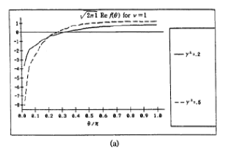
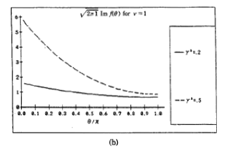
Figure 1: The scattering amplitude for $\nu=1$ and $\gamma\neq 0$. (a) $(2\pi l)^{1/2}{\rm Re}f(\theta)$, (b) $(2\pi l)^{1/2}{\rm Im}f(\theta)$. The solid line stands for $\gamma^{2}=0.2$ and the broken line for $\gamma^{2}=0.5$.

The $S$-wave ($n=0$) contribution in the formula (16) gives

$$(2\pi l)^{1/2}{\rm Re}f_{0} = -2\sin(\pi\gamma/2)\cos(\pi\gamma/2)\,,$$ (22)

$$(2\pi l)^{1/2}{\rm Im}f_{0} = 2\sin^{2}(\pi\gamma/2)\,,$$ (23)

and these seem to be a good estimation as the lowest order.

The optical theorem

$${\rm Im}f(0)=(l/8\pi)^{1/2}\int_{0}^{2\pi}|f(\theta)|^{2}d\theta\,,$$ (24)

is applicable for $\nu=1$ and one can confirm this at the order in using the $S$-wave result (22, 23). Note that the amplitude does not contain divergences for $\nu=1$ (for instance, delta functions cancel one another in (19) when $\nu=1$.).

Although the potential has a short-range nature, the Born approximation is not applicable because the singularity near the origin is too strong.

Next we consider the case for a cosmic string. Here we recover the relation $\gamma^{2}=e^{2}(\nu 2-1)/24\pi^{2}$. We define $\Delta f$ by the difference in the scattering amplitudes for $\gamma^{2}=e^{2}(\nu 2-1)/24\pi^{2}$ and $\gamma^{2}=0$; i.e., the contribution of (19) is subtracted. The numerical results are given in Fig. 2. The value of ${\rm Im}\Delta f$ in the vicinity of $(\nu-1)\pi$ is not indicated because of the poor convergence in the sum of the oscillating series. The value seems almost constant.

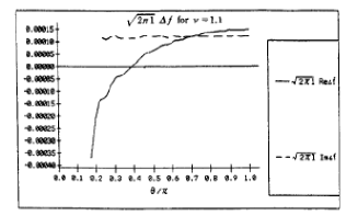
Figure 2: The difference in the scattering amplitudes for $\gamma^{2}=e^{2}(\nu^{2}-I)/24\pi^{2}$ and $\gamma^{2}=0$ in the case of $\nu-1=0.1$. We set $e^{2}/4\pi=1/137$. The solid line stands for $(2\pi l)^{1/2}{\rm Re}\Delta f$ and the broken line for $(2\pi l)^{1/2}{\rm Im}\Delta f$.

The real part of $\Delta f$ exhibits a logarithmical divergence at $\theta=(\nu-1)\pi$. The behavior of the amplitude is approximately given by:

$$(2\pi l)^{1/2}{\rm Re}\Delta f=-2\sin(\pi\gamma/2)\cos(\pi\gamma/2)$$

$$\qquad+\frac{\pi\gamma^{2}}{2\nu}\ln\left|4\sin\frac{\theta+(\nu-1)\pi}{2}\sin\frac{\theta-(\nu-1)\pi}{2}\right|+O(\gamma^{4})\,,$$ (25)

$$(2\pi l)^{1/2}{\rm Im}\Delta f=2\sin^{2}(\pi\gamma/2)$$

$$\qquad+\frac{\pi\gamma^{2}}{2\nu}\left\{\nu-1-\left\{\begin{array}[]{cc}1&(\theta<(\nu-1)\pi)\\ 0&((\nu-1)\pi<\theta)\end{array}\right\}\right\}+O(\gamma^{4})\,.$$ (28)

For a realistic cosmic string, $\nu-1$ may be too small for us to detect the deviation in the scattering amplitude unless the strength of the coupling become sufficiently large.

5 Conclusion

In this paper we have derived the lowest-order vacuum quantum space electromagnetic corrections to the scattering amplitude in a conical background space-time. Inclusion of the quantum effect of non-Abelian gauge fields around a cosmic string is an important extension of the present work: it may be connected with non-Abelian AB effect [9] and the baryon decay/genesis mediated by cosmic strings.[10] It is also important to treat the effect of self-interaction in a conical space for the Yang-Mills case. (Self-interacting scalar fields around a cosmic string have been studied in ref. [11].).

References

- [1] J. S. Dowker, Phys. Rev. D36 (1987) 3742.
- [2] V. P. Frolov and E. M. Serebriany, Phys. Rev. D35 (1987) 3779.
- [3] B. Linet, Phys. Rev. D35 (1987) 536.
- [4] A. G. Smith, in The formation and evolution of cosmic strings, eds. by G. Gibbons, S. Hawking and T. Vachaspati (Cambridge Univ., Cambridge, 1990).
- [5] G. ’t Hooft, Commun. Math. Phys. 117 (1988) 685; S. Deser and R. Jackiw, Commun. Math. Phys. 118 (1988) 495; P. de Sousa Gerbert and R Jackiw, Commun. Math. Phys. 124 (1989) 229; G. W. Gibbons, F. Ruiz and T. Vachaspati, Commun. Math. Phys. 127 (1990) 295.
- [6] K. Shiraishi, in preparation.
- [7] E. Witten, Nucl. Phys. B249 (1985) 557.
- [8] I. R. Lapidus, Am. J. Phys. 50 (1982) 45; P. A, Maurone and T. K. Lim. Am. J. Phys. 51 (1983) 856; J. F. Perez and F. A. B. Coutinho, Am. J. Phys. 59 (1991) 52; G. T. Barton, Am. J. Phys. 51 (1983) 420.
- [9] P. A. Horvathy, Phys. Rev. D33 (1986) 407; M. G. Alford, J. March-Russell and F. Wilczek, Nucl. Phys. B337 (1990) 695; M. G. Alford, A. Benson, S. Coleman, J. March-Russell and F. Wilczek, Phys. Rev. Lett. 64 (1990) 1632; Nucl. Phys. B349 (1991) 414; F. Wilczek and Y.-S. Wu, Phys. Rev. Lett. 65 (1990) 13; M. Bucher, Nucl. Phys. B350 (1991) 163.
- [10] R. H. Brandenberger and L. Perivolaropoulos, Phys. Lett. B208 (1988) 396; R H. Brandenberger, A.-C. Davis and A. M. Matheson, Phys. Lett. B218 (1989) 304; A.-C. Davis and W. Perkins, Phys. Lett. B228 (1989) 37; R. H. Brandenberger, A.-C. Davis and A. M. Matheson, Nucl. Phys. B307 (1988) 909; R. Gregory, A.-C. Davis and R. H. Brandenberger, Nucl. Phys. B323 (1989) 187; L. Perivolaropoulos. A. Matheson, A.-C. Davis and R. H. Brandenberger, Phys. Lett. B245 (1990) 556; A. Matheson, L. Perivolaropoulos, W. Perkins, A.-C. Davis and R. H. Brandenberger, Phys. Lett. B248 (1990) 263; A. Matheson, Mod. Phys. Lett. A6 (1991) 769; W. B. Perkins, L. Perivolaropoulos, A.-C. Davis, R. H. Brandenberger and A. Matheson, Nucl. Phys. B353 (1991) 237; M. G. Alford, J. March-Russell and F. Wilczek, Nucl. Phys. 328 (1989) 140.
- [11] I. H. Russell and D. J. Toms, Class. Q. Grav. 6 (1989) 1343; K. Shiraishi and S. Hirenzaki, Class. Q. Grav. 9 (1992) 2277.
- [12] A. D. Linde, Rep. Prog. Phys. 42 (1979) 389, and references there in.