Dynamics of social contagions with heterogeneous adoption thresholds: Crossover phenomena in phase transition

Abstract

Heterogeneous adoption thresholds exist widely in social contagions, but were always neglected in previous studies. We first propose a non-Markovian spreading threshold model with general adoption threshold distribution. In order to understand the effects of heterogeneous adoption thresholds quantitatively, an edge-based compartmental theory is developed for the proposed model. We use a binary spreading threshold model as a specific example, in which some individuals have a low adoption threshold (i.e., activists) while the remaining ones hold a relatively high adoption threshold (i.e., bigots), to demonstrate that heterogeneous adoption thresholds markedly affect the final adoption size and phase transition. Interestingly, the first-order, second-order and hybrid phase transitions can be found in the system. More importantly, there are two different kinds of crossover phenomena in phase transition for distinct values of bigots’ adoption threshold: a change from first-order or hybrid phase transition to the second-order phase transition. The theoretical predictions based on the suggested theory agree very well with the results of numerical simulations.

I Introduction

Social contagions are ubiquitous in human society, and generate new scientific challenges for network science Watts2007 ; Castellano2009 . All the researches about sentiments contagion, information spreading and behavior spreading fall into the category of studying social contagions Christakis2007 ; Barrat2008 . In particular, behavior spreading, as a representative and essential type of social contagions, has attracted great attention, both theoretically and experimentally Centola2011 ; Banerjee2013 . Understanding the spreading mechanisms behind behavior has the potential to not only help us design better anti-virus strategies Pastor-Satorras2014 , but also shed new insights into the control of social unrest Watts2007 . Moreover, different from biological contagions (such as epidemic spreading) Moreno2002 ; Pastor-Satorras2001 ; Salathe2011 ; Yang2015b ; Yang2011 ; Li2014 , social contagions display one inherent characteristic: social reinforcement effect Pastor-Satorras2014 ; Porter2014 , which usually plays a vital role in the final status of contagions.

To examine social reinforcement effect, some successful models have been proposed Watts2002 ; Granovetter1973 , most of which assume that all individuals have the same adoption threshold to incorporate such an effect (so-called threshold model). That is to say, each individual adopts the behavior only when the fraction Watts2002 or number Granovetter1973 of neighbors with the adopted state exceeds his adoption threshold. In this case, the social contagions is a trivial case of Markovian process. By means of numerical simulations and theoretical analysis, it was found that the social reinforcement effect can evidently change the phase transitions of contagion dynamics. More specifically, the final adoption size first grows continuously and then decreases discontinuously with the increase of mean degree when the adoption threshold of all individuals is identical Watts2002 . After this seminal discovery, the role of threshold model and its various underlying mechanisms, in social contagions have been intensively explored, including the influence of dynamical parameters (e.g., initial seeds and threshold sizes Gleeson2007 ; Singh2013 ), and topology characteristics (degree-degree correlations Dodds2009 , clustering Whitney2007 ; Gleeson2008 , community structure Nematzadeh2014 as well as multiplexity framework Brummitt2012 ; Yagan2013 ), which are the primary factors in determining the final adoption size and phase transition. Some non-Markovian social contagion models were also proposed to describe the social reinforcement effect Dodds2004 ; Wang2015 ; Zheng2013 . For example, in a recent research paper Wang2015 , where the social reinforcement was derived from the memory of non-redundant information transmission, it was found that the perturbation of dynamical or structural parameters makes the dependence of final behavior adoption size on information transmission probability change from being discontinuous to being continuous. In Ref. Zheng2013 , Zheng et al. further verified that the role of social reinforcement in behavior diffusion on regular graphs and online social networks, which is consistent with early experimental anticipation Centola2010

Recently, researchers found that the widely existed individual heterogeneity dramatically alters the spreading dynamics. In epidemic spreading, the heterogeneous infectivity and susceptibility can change the outbreak threshold Miller2008 ; Yang2015 . For information spreading, the heterogeneous waiting and response time may speed up or slow down the velocity of information diffusion Cui2014 ; Jo2014 . Statistical physicists found that individual heterogeneity can induce the hybrid phase transition Wu2014 ; Hu2011 , which mixes the traditional first-order and second-order transitions, in k-core percolation Cellai2011 and bootstrap percolation Gleeson2007 ; Baxter2011 ; Lee2014 . In practical behavior spreading, individuals usually show different wills to mimic the behavior, which means that each agent owns his own adoption threshold Karsai2014 . Some individuals with low adoption threshold show strong wills to adopt the behavior and act as activists. Nevertheless, others with high adoption threshold need to capture more behavioral information before imitation, and they often act as bigots. With regard to the difference of adoption threshold, it may be closely related with personal interests, education background, or other personality and social factors Watts2007 . For example, the well-educated population is more likely to adopt the high-tech products than that among the populations who lacks the basic education. Similarly, students are more likely to adopt an interesting computer game than housewives.

Unfortunately, there is still absence of systematical understanding about the role of heterogeneous adoption thresholds in social contagions. Aiming to resolve this issue, we will explore how heterogeneous adoption thresholds affect the final adoption size and phase transition of social contagions based on a so-called binary spreading threshold model, which is a non-Markovian process. Meanwhile, an edge-based compartmental theory is developed for quantitative validation. Interestingly, it is found that heterogeneous adoption thresholds significantly affect the final adoption size, and generate the hierarchical characteristic of adopting behavior: activists first adopt the given behavior themselves, and then stimulate bigots to follow this behavior. Moreover, it is worth noting that such a heterogeneous threshold model results in the existence of first-order, seconde-order and hybrid phase transitions. More importantly, there are two different kinds of crossover phenomena in phase transition for distinct values of the bigots’ adoption threshold: a change from first-order or hybrid phase transitions to the second-order phase transition. In what follows, we will first describe the heterogeneous social contagion model in complex networks, followed by the description of edge-based compartmental theory, and then represent the simulation and analysis results. Finally, we will draw our conclusions.

II Social contagion model with heterogeneous adoption thresholds

Behavior spreading on complex networks is considered with $N$ nodes and the degree distribution $P(k)$. As the interaction networks, we use the configuration model Catanzaro2005 to avoid the additional influence of degree-degree correlations. Nodes in the network represent individuals and edges between nodes stand for the contacts with which behavioral information transmission may occur. For each individual, a static behavioral adoption threshold is assigned according to a specific distribution function $F(T)$, which is independent of network topology. The larger value of $T$ means that an individual needs to capture more behavioral information from his neighbors before adopting the behavior.

With regard to behavior spreading dynamics, we generalize the spreading threshold model with social reinforcement derived from memory of non-redundant information transmission characters Wang2015 ; Wang2015b . In this model, each individual falls into one of the three states: susceptible (S), adopted (A) and recovered (R) (namely, susceptible-adopted-recovered, SAR model). In the susceptible state, an individual does not adopt the behavior. In the adopted state, an individual adopts the behavior and tries to transmit the behavioral information to his neighbors. In the recovered state, an individual loses interest in the behavior and will not transmit the behavioral information further. Initially, a vanishingly small fraction of individuals $\rho_{0}$ are chosen as seeds (adopters) at random, while the others are fixed in the susceptible state.

At each time step, each adopted individual $v$ tries to diffuse the behavioral information to every susceptible neighbor with probability $\lambda$. In particular, once the information is transmitted through an edge successfully, it will never be transmitted again, i.e., only non-redundant information transmission is allowed. If the susceptible neighbor $u$ of $v$ is successfully informed, his cumulative pieces of information $m$ add $1$ (i.e., $m=m+1$). Subsequently, individual $u$ compares the new value of $m$ with his adoption threshold $T_{u}$, and becomes an adopter once $m\geq T_{u}$. Obviously, whether an individual adopts the behavior is determined by the cumulative pieces of behavioral information he ever received from distinct neighbors. Thus, the non-Markovian effect is induced in the behavior spreading dynamics. After information transmission, individual $v$ may lose interest in the behavior with probability $\gamma$ and then moves into the recovered state. Individuals falling into the recovered state will stop from participating in the further behavioral information spreading, and the spreading dynamics terminate when all adopted individuals become recovered.

III Edge-based compartmental theory

In order to describe the strong dynamical correlations among the states of neighbors in heterogeneous social contagion model, an edge-based compartmental approach is established herein, which is inspired by Refs. Miller2011 ; Miller2013 ; Wang2014 . Correspondingly, the notations $S(t)$, $A(t)$ and $R(t)$ respectively represent the fraction of individuals in the susceptible, adopted, and recovered states at time step $t$.

III.1 General adoption threshold distribution

Individual $u$ is set to be in the cavity state, which means that he can receive behavioral information from neighbors but not transmit behavioral information to his neighbors Karra2010 . Define $\theta(t)$ as the probability that individual $v$ has not transmitted the behavioral information to individual $u$ along a randomly chosen edge by time $t$. Thus, the probability that an individual $u$ with degree $k$ has received $m$ pieces of behavioral information from distinct neighbors by time $t$ can be expressed as

$$\phi_{m}(k,t)=\binom{k}{m}[\theta(t)]^{k-m}[1-\theta(t)]^{m}.$$ (1)

Individual $u$ in the susceptible state implies that the cumulative pieces of behavioral information $m$ he received are still less than his adoption threshold $T_{u}$. According to the social contagion model in Sec. II, the adoption threshold and degree are independent. Considering all possible values of $m$ and $T_{u}$, it can be obtained that the probability of individual $u$ with degree $k$ being susceptible is

$$s(k,t)=\sum_{T_{u}}F(T_{u})\sum_{m=0}^{T_{u}-1}\phi_{m}(k,t).$$ (2)

Combing the degree distribution of a network, the fraction of susceptible individuals at time step $t$ is

$$S(t)=\sum_{k}P(k)s(k,t).$$ (3)

It is obvious that $S(t)$ can be figured out after $\theta(t)$ is known.

As a neighbor of individual $u$ may be in one of susceptible, adopted or recovered state, $\theta(t)$ can be divided into three cases as

$$\theta(t)=\xi_{S}(t)+\xi_{A}(t)+\xi_{R}(t).$$ (4)

And $\xi_{S}(t)$ [$\xi_{A}(t)$ or $\xi_{R}(t)$] denotes that the susceptible (adopted or recovered) neighbor $v$ of $u$ has not transmitted the behavioral information to individual $u$ up to time $t$.

Then, let’s explore the above three terms. If individual $v$ with degree $k^{\prime}$ is susceptible initially, he can not transmit the behavioral information to $u$, but only receive it from other $k^{\prime}-1$ neighbors since $u$ in a cavity state. Thus, the probability that individual $v$ has received $m$ pieces of behavioral information by time $t$ is

$$\tau_{m}(k^{\prime},t)=\binom{k^{\prime}-1}{m}[\theta(t)]^{k^{\prime}-m-1}[1-\theta(t)]^{m}.$$ (5)

Taking all possible values of $m$ and $T_{v}$ into consideration, the probability of individual $v$ remaining in susceptible state becomes [similar to Eq. (2)]

$$\Theta(k^{\prime},t)=\sum_{T_{v}}F(T_{v})\sum_{m=0}^{T_{v}-1}\tau_{m}(k^{\prime},t).$$ (6)

The probability of an edge connecting an individual with degree $k^{\prime}$ is $k^{\prime}P(k^{\prime})/\langle k\rangle$ for uncorrelated networks, where $\langle k\rangle$ is the mean degree. Thus, it can be obtained that

$$\xi_{S}(t)=\frac{\sum_{k^{\prime}}k^{\prime}P(k^{\prime})\Theta(k^{\prime},t)}{\langle k\rangle}.$$ (7)

Subsequently, we turn to the expressions of $\xi_{A}(t)$ and $\xi_{R}(t)$. Once the behavioral information is transmitted through an edge with probability $\lambda$, the edge will no longer satisfy the definition of $\theta(t)$. Thus, the rate of flow from $\theta(t)$ to $1-\theta(t)$ is $\lambda\xi_{A}(t)$, which can be expressed as

$$\frac{d\theta(t)}{dt}=-\lambda\xi_{A}(t).$$ (8)

For the growing of $\xi_{R}(t)$, two events conditions must be met simultaneously. At time $t$, the behavioral information does not transmit through an edge with probability $1-\lambda$, and the adopted individual enters recovered state with probability $\gamma$. Then,

$$\frac{d\xi_{R}(t)}{dt}=\gamma(1-\lambda)\xi_{A}(t).$$ (9)

Combining Eqs. (8) and (9), one has that

$$\xi_{R}(t)=\frac{\gamma[1-\theta(t)](1-\lambda)}{\lambda}.$$ (10)

Inserting Eqs. (7) and (10) into Eq. (4), the following expression can be obtained that

$$\xi_{A}(t)=\theta(t)-\frac{\sum_{k^{\prime}}k^{\prime}P(k^{\prime})\Theta(k^{\prime},t)}{\langle k\rangle}-\frac{\gamma[1-\theta(t)](1-\lambda)}{\lambda}.$$ (11)

Substituting Eq. (11) into Eq. (8), we get the time evolution of $\theta(t)$ in details

$$\frac{d\theta(t)}{dt}=-\lambda[\theta(t)-\frac{\sum_{k^{\prime}}k^{\prime}P(k^{\prime})\Theta(k^{\prime},t)}{\langle k\rangle}]+\gamma[1-\theta(t)](1-\lambda).$$ (12)

Susceptible individuals move into the adopted states once they adopt the behavior, meanwhile the adopted individuals may lose interest in the behavior and become recovered. Thus, we can easily get the evolution of adopted and recovered individuals as

$$\frac{dA(t)}{dt}=-\frac{dS(t)}{dt}-\gamma A(t)$$ (13)

and

$$\frac{dR(t)}{dt}=\gamma A(t),$$ (14)

respectively. Eqs. (1)-(3) and (12)-(14) give us a complete and general description of heterogeneous social contagions, from which the fraction in each state at arbitrary time step can be calculated. When $t\rightarrow\infty$, we can get the final adoption size $R(\infty)$.

III.2 Binominal adoption threshold distribution

In this subsection, we pay attention to the behavior adoption threshold with a binominal distribution $F(T)$. More specifically, a fraction of individuals $p$ have a relatively low adoption threshold $T_{a}$, whereas the remaining individuals have a high adoption threshold $T_{b}$. $F(T)$ can be expressed as

$$F(T)=\left\{\begin{array}[]{rcl}{T_{a},}&{\mathrm{with~{}probability}~{}p,}\\ {T_{b},}&{\mathrm{with~{}probability}~{}1-p.}\end{array}\right.$$ (15)

For simplicity, the values of adoption thresholds are defined as $T_{a}=1$ and $T_{b}\geq 1$. Individuals with low adoption threshold $T_{a}$ are considered as activists, while those with high adoption threshold $T_{b}$ are regarded as bigots. We herein name this kind of social contagion model as binary spreading threshold model. And the edge-based compartmental theory is utilized to analyze the binary spreading threshold model by substituting Eq. (15) into various equations that give the solutions of $S(t)$, $A(t)$ and $R(t)$. Particularly, we rewrite Eqs. (2) and (6) as

$$s(k,t)=p\theta(t)^{k}+(1-p)\sum_{m=0}^{T_{b}-1}\phi_{m}(k,t),$$ (16)

and

$$\Theta(k^{\prime},t)=p\theta(t)^{k^{\prime}-1}+(1-p)\sum_{m=0}^{T_{b}-1}\tau_{m}(k^{\prime},t),$$ (17)

respectively. At time $t$, the fractions of susceptible individuals in the activist and bigot populations are given by

$$S_{l}(t)=\sum_{k}P(k)\theta(t)^{k},$$ (18)

and

$$S_{h}(t)=\sum_{k}P(k)\sum_{m=0}^{T_{b}-1}\phi_{m}(k,t),$$ (19)

respectively. Considering the fractions of the activist and bigot populations, the density of susceptible individuals at time step $t$ can also be written as

$$S(t)=pS_{l}(t)+(1-p)S_{h}(t).$$ (20)

The effects of heterogeneous adoption threshold on phase transition is another issue concerned. To analyze the phase transition, we can address the fixed point (root) of Eq. (12) at the steady state (i.e., $t\rightarrow\infty$) with Eq. (17). That is the fixed point of

$$\theta(\infty)=y[\theta(\infty)],$$ (21)

where

$$y[\theta(\infty)]=\frac{\sum_{k^{\prime}}k^{\prime}P(k^{\prime})\Theta(k^{\prime},\infty)}{\langle k\rangle}+\frac{\gamma[1-\theta(\infty)](1-\lambda)}{\lambda}.$$ (22)

From Fig. 1(a), it can be seen that the number of nontrivial roots is either $0$, $1$ or $3$ when $T_{b}\geq 3$. With $T_{b}=2$, the number of nontrivial roots is either $0$, $1$ or $2$ [see Fig. 1(b)].

III.2.1 Case of $T_{b}\geq 3$

In this subsection, we discuss the case of $T_{b}\geq 3$. For the given $P(k)$, $p$ and $\gamma$, Eq. (21) has only one trivial solution $\theta(\infty)=1$ when $\lambda$ is small. With the increase of $\lambda$, $\theta(\infty)$ decreases continuously to a nontrivial solution $\theta(\infty)<1$ first [see example in Fig. 1(a)], which means that $R(\infty)$ grows continuously first. That is to say, there is a second-order (continuous) phase transition. By setting $\theta(\infty)$ and $y[\theta(\infty)]$ tangent at $\theta(\infty)=1$ Hu2011 ; Newman2001 , we get the continuous critical information transmission probability as

$$\lambda_{c}^{II}=\frac{\gamma\langle k\rangle}{p(\langle k^{2}\rangle-\langle k\rangle)-(1-\gamma)\langle k\rangle},$$ (23)

where $\langle k\rangle$ and $\langle k^{2}\rangle$ are the first and second moments of degree distribution, respectively. The critical value $\lambda_{c}^{II}$ separates the local behavior adoption (i.e., the behavior can be adopted by a vanishingly small fraction of individuals) from the global behavior adoption (i.e., the behavior can be adopted by a finite fraction of individuals). From Eq. (23), it is discovered that the occurrence of global behavior adoption is determined by the network topology (i.e., degree distribution), the fraction of activists $p$ and the recovery probability $\gamma$. The global behavior adoption is more likely outbreak (i.e., a lower $\lambda_{c}^{II}$) for scale-free networks with divergent second moment degree distribution [i.e., $\langle k^{2}\rangle\rightarrow\infty$]. Increasing the value of $p$ can facilitate the global behavior adoption (i.e., a lower $\lambda_{c}^{II}$). When $p=1$, Eq. (23) returns to the case of epidemic outbreak threshold Wang2014 .

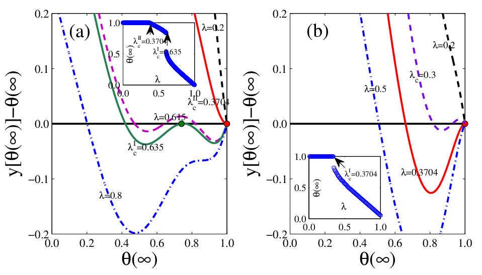
Figure 1: (Color online) Illustration of graphical solutions of Eq. (21) when $T_{b}=4$ (a) and $T_{b}=2$ (b) on random regular networks. In (a) and (b), the black solid lines represent the horizontal axis and the red and green dots denote the tangent points. The inset of (a) and (b) shows the physically meaningful solutions of Eq. (21) when $T_{b}=4$ and $T_{b}=2$, respectively. And the arrows indicate critical transmission probabilities. The fixed points of Eq. (21) are the intersections between the curve and horizontal axis. Other parameters are defined $p=0.3$ and $\langle k\rangle=10$.

Fixing all the parameters except $p$, similar to Eq. (23), we get the continuous critical fraction of activists as

$$p_{c}^{II}=\frac{\gamma\langle k\rangle}{\lambda(\langle k^{2}\rangle-\langle k\rangle)}+\frac{(1-\gamma)\langle k\rangle}{\langle k^{2}\rangle-\langle k\rangle}.$$ (24)

From Eq. (24), it can be known that an enough fraction of activists are necessary for triggering the global behavior adoption, and $p_{c}^{II}$ decreases with the increase of network heterogeneity, $p$ and $\lambda$. By setting $\gamma=0$ in Eq. (24), another critical proportion of activists $p_{c}^{\star}$ can be obtained, below which any values of $\lambda$ can not trigger the global behavior adoption, which is given by

$$p_{c}^{\star}=\frac{\langle k\rangle}{\langle k^{2}\rangle-\langle k\rangle}.$$ (25)

It is worth noting that Eq. (25) is the same with network’s percolation condition Newman2001 , which means that the global behavior adoption is possible only when the activists percolate the entire network (i.e., activists can form a finite connected cluster).

As shown in Fig. 1(a), three nontrivial roots of Eq. (21) occur when $\lambda$ is large enough [see Fig. 1(a) for $\lambda=0.615$]. This phenomenon is caused by the bigots, since Eq. (21) has at most one nontrivial root when the bigots is absent Wang2015 . In this case, the meaningful solution will be given by the largest stable root (since only this value can be achieved physically). For $\lambda=\lambda_{c}^{I}=0.635$, the tangent point is the solution. For $\lambda>\lambda_{c}^{I}$, the meaningful solution is the only stable fixed point. The meaning solution of Eq. (21) changes abruptly to a small value from a relatively large value at $\lambda_{c}^{I}$ [see the insert Fig. 1(a)], and resulting in a discontinuous growth of $R(\infty)$. Based on bifurcation theory Strogatz1994 , the discontinuous critical information transmission probability is gained as follows

$$\lambda_{c}^{I}=\frac{\gamma}{\Delta+\gamma-1},$$ (26)

where

$$\Delta=\frac{\sum_{k^{\prime}}k^{\prime}P(k^{\prime})\frac{d\Theta(k^{\prime},\infty)}{d\theta(\infty)}|_{\theta_{s}(\infty)}}{\langle k\rangle},$$

and $\theta_{s}(\infty)$ is the fixed point of Eq. (21). Combining Eqs. (5) and (17), we get

$$\frac{d\Theta(k^{\prime},\infty)}{d\theta(t)}=p(k^{\prime}-1)\theta(\infty)^{k^{\prime}-2}+(1-p)\mathcal{X},$$ (27)

where

$$\begin{split}\mathcal{X}&=\sum_{m=0}^{T_{b}-1}\binom{k^{\prime}-1}{m}\{(k^{\prime}-m-1)\theta(\infty)^{k^{\prime}-m-2}[1-\theta(\infty)]^{m}\\ &-m\theta(\infty)^{k^{\prime}-m-1}[1-\theta(\infty)]^{m-1}\}.\end{split}$$ (28)

Using the analytical method similar to Eq. (26), the discontinuous critical fraction of activists can be expressed as

$$p_{c}^{I}=\frac{\lambda(1-\mathcal{Y})+\gamma(1-\lambda)}{\lambda(\mathcal{Z}-\mathcal{Y})},$$ (29)

where

$$\mathcal{Y}=\frac{\sum_{k^{\prime}}k^{\prime}P(k^{\prime})\mathcal{X}}{\langle k\rangle}$$

and

$$\mathcal{Z}=\frac{\sum_{k^{\prime}}k^{\prime}(k^{\prime}-1)P(k^{\prime})\theta^{k^{\prime}-2}}{\langle k\rangle}.$$

From the above analysis, we find that $R(\infty)$ versus $\lambda$ or $p$ first grows continuously and then follows a discontinuous fashion. And the continuous and discontinuous growthes of $R(\infty)$ are caused by the activists and bigots, respectively, which can be regarded as hybrid phase transition, mixing the traditional first-order and second-order transitions, from the perspective of statistical physics Dorogovtsev2008 . Note that the hybrid phase transition can change to a second-order phase transition, and does not exist under any conditions. Numerically solving Eqs. (21), (26), and the following equation

$$\frac{d^{2}g[\theta(\infty)]}{d\theta^{2}(\infty)}=0,$$ (30)

we can learn the condition under which the hybrid phase transition disappears.

III.2.2 Case of $T_{b}=2$

We study the special case of $T_{b}=2$ in this subsection. As shown in Fig. 1(b), for any $\lambda$, $y[\theta(\infty)]$ can only tangent to $\theta(\infty)$ when $\theta(\infty)=1$, and can not tangent to other $\theta(\infty)<1$. In addition, Eq. (21) has $1$ or $2$ nontrivial fixed points. These phenomena means that the meaningful solution of Eq. (21) jumps to another one at the critical information transmission probability [see the inset of Fig. 1(b)]. As a result, $R(\infty)$ increases discontinuously versus $\lambda$. The critical information transmission probability can be acquired in the similar way as when $T_{b}=3$. The values of $\lambda_{c}^{II}$ and $\lambda_{c}^{I}$ can be obtained from Eq. (23), since $y[\theta(\infty)]$ can only tangent to $\theta(\infty)$ when $\theta(\infty)=1$. Numerical solving Eqs. (21), (26) and (30), we can get the condition under which the first-order phase transition changes to a second-order phase transition.

IV Numerical verification

In the study, extensive simulations are conducted for on binary spreading threshold model on uncorrelated networks. Unless otherwise specified, the network size, mean degree and recovery probability are of $N=10,000$, $\langle k\rangle=10$ and $\gamma=1.0$, respectively. At least $2\times 10^{3}$ independent dynamical realizations on a fixed network are used to calculate the pertinent average values, which are further averaged over $100$ network realizations.

The relative variance $v_{R}$ is applied to numerically determine the size-dependent critical values, such as, $\lambda_{c}^{I}$, $\lambda_{c}^{II}$, $p_{c}^{I}$ and $p_{c}^{II}$. The relative variance of $R(\infty)$ is defined as

$$v_{R}=\frac{\langle R(\infty)-\langle R(\infty)\rangle\rangle^{2}}{\langle R(\infty)\rangle^{2}},$$ (31)

where $\langle\cdots\rangle$ denotes ensemble averaging. The value of $v_{R}$ exhibits peaks at the phase transition, which announce the phase transition Chen2014 . We determine the critical value $\omega_{c}$, which represents $\lambda_{c}^{I}$, $\lambda_{c}^{II}$, $p_{c}^{I}$ or $p_{c}^{II}$, as the value of $\lambda$ or $p$ when the relative variance reaches its maximum, and

$$\omega_{c}=\mathrm{arg}\{\mathrm{max}~{}v_{R}\}.$$ (32)

Note that Eq. (32) is not the only possible way to compute the critical values, other methods can be used to determine $\omega_{c}$, such as, susceptibility Radicchi2014 ; Ferreira2012 and variability Shu2014 .

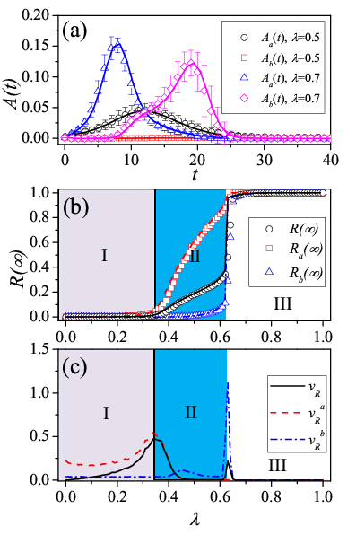
Figure 2: (Color online) Binary spreading threshold model on random regular networks. (a) Average density of adopted individuals $A_{a}(t)$ and $A_{b}(t)$ versus time $t$ in the activist and bigot populations with different information transmission probability $\lambda$. The error bars indicate the standard deviations. (b) Final adoption size $R(\infty)$ and (c) relative variance $v_{R}$ versus $\lambda$ for full, activist and bigot populations. In figures (a) and (b), symbols represent the simulated results, and the lines are the corresponding theoretical predictions from Eqs. (12)-(14) and (16)-(20). Lines in (c) are the simulation results of $v_{R}$. In (b) and (c), the vertical lines are the critical continuous and discontinuous information transmission probabilities, which are denoted as $\lambda_{c}^{II}$ and $\lambda_{c}^{I}$, respectively. The theoretical values of $\lambda_{c}^{II}$ and $\lambda_{c}^{I}$ can be gotten from Eqs. (23) and (26), respectively. The theoretical (numerical) values of $\lambda_{c}^{II}$ and $\lambda_{c}^{I}$ separate (b) [(c)] into three regions. Region I, only a vanishingly small fraction of individuals can be exposed to adopt the behavior; region II, only a finite fraction of activists adopt the behavior; region III, a finite fraction of activists and bigots adopt the behavior. Other parameters are set to be $N=10,000$, $p=0.3$ and $T_{b}=4$.

IV.1 Random regular networks

To be illustrative, we first focus on random regular networks (RRNs). Fig. 2(a) shows the time evolution of the fraction of adopted individuals $A_{a}(t)$ and $A_{b}(t)$ in the activist and bigot populations with different behavioral information transmission probabilities $\lambda$. It is found that a hierarchical character of behavior adoption is caused by heterogeneous adoption thresholds. That is to say, activists with low $T_{a}$ first adopt the behavior and then stimulate the bigots with $T_{b}$ to adopt the behavior. With a relatively small $\lambda=0.5$, $A_{a}(t)$ shows a small peak, and can not stimulate a finite fraction of bigots to adopt the behavior [$A_{b}(t)$ does not see an obvious peak]. With a relatively large $\lambda=0.7$, $A_{a}(t)$ shows a large peak, and further causing the emergence of a large peak for $A_{a}(t)$. The heterogeneous adoption threshold distribution may be used to explain the existence of multimodal in the adoption of serves Karsai2014 . The time evolution can be well predicted by our edge-based compartmental theory.

From Figs. 2(b) and (c), it can be seen that $R(\infty)$ versus $\lambda$ shows a hybrid phase transition, which means that $R(\infty)$ first grows continuously and then follows a discontinuous fashion. The continuous and discontinuous phase transitions are caused by activists and bigots, respectively. Similar to Ref. Wang2015 , the discontinuous growth of $R(\infty)$ is caused by those bigots in the subcritical state who adopt the behavior simultaneously. An individual in such a state has received the behavioral information but has not yet adopted the behavior, and the number of information pieces from distinct neighbors is precisely one less than his adoption threshold. The theoretical (numerical) values of $\lambda_{c}^{II}$ and $\lambda_{c}^{I}$ separate Figs. 2(b) [(c)] into three regions. The theoretical values of $\lambda_{c}^{II}$ and $\lambda_{c}^{I}$ can be gotten from Eqs. (23) and (26), respectively. In region I, with $\lambda\leq\lambda_{c}^{II}$, both activist and bigot populations adopt the behavior locally (i.e., only a vanishingly small fraction of individuals adopted the behavior). In region II, with $\lambda_{c}^{II}<\lambda\leq\lambda_{c}^{I}$, activists adopt the behavior globally (i.e., a finite fraction of activists adopted the behavior) and bigots adopt the behavior locally. In region III with $\lambda>\lambda_{c}^{I}$, both the activists and bigots adopt the behavior globally. The numerical values of $\lambda_{c}^{II}$ and $\lambda_{c}^{I}$ can be obtained by observing $v_{R}$ in Fig. 2(c). For instance, $v_{R}$ has two peaks, which means that two phase transitions occur Chen2014 . And the first peak appears at $\lambda_{c}^{II}$, while the second peak locates at $\lambda_{c}^{I}$. Note that the first (second) peak of $v_{R}$ shares the same location with the maximal peak of activist population $v_{R}^{a}$ (bigots population $v_{R}^{b}$). In all, $\lambda_{c}^{I}$, $\lambda_{c}^{II}$ and $R(\infty)$ can be well predicted by our edge-based compartmental theory.

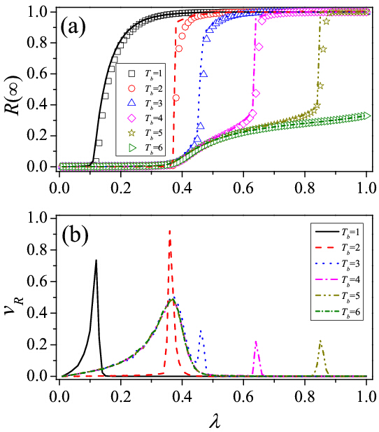
Figure 3: (Color online) Effects of bigots’ adoption threshold on binary spreading threshold model. (a) $R(\infty)$ and (b) $v_{R}$ versus $\lambda$ with different $T_{b}$. In figure (a), symbols represent the simulated results, and the lines are the theoretical predictions from Eqs. (12)-(14) and (16)-(20). In figure (b), lines are the simulation results of $v_{R}$, and we plot the value of $v_{R}/20$ for $T_{b}=2$. Other parameters are defined as $N=10,000$ and $p=0.3$.

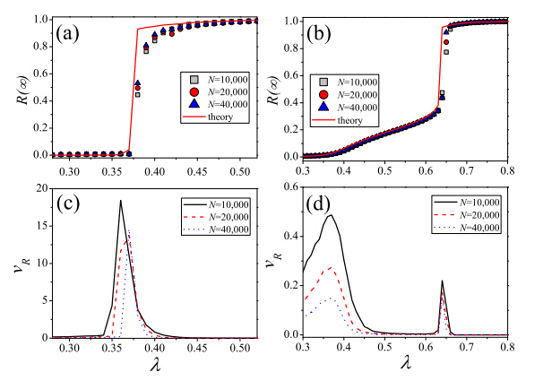
Figure 4: (Color online) Finite-size effects on the binary spreading threshold model for $p=0.3$. (a) $R(\infty)$ and (c) $v_{R}$ versus $\lambda$ for $T_{b}=2$ on different network size $N$. (b) $R(\infty)$ and (d) $v_{R}$ versus $\lambda$ for $T_{b}=4$ under different $N$. The lines in (a) and (b) are the theoretical predictions from Eqs. (12)-(14) and (16)-(20). The lines in (c) and (d) are the simulation results of $v_{R}$.

As shown in Fig. 3, $R(\infty)$ and the phase transition are significantly influenced by the adoption threshold of bigots $T_{b}$. And $R(\infty)$ decreases with $T_{b}$, since a larger value of $T_{b}$ requires more information to be exposed for bigots. The phase transition is continuous when $T_{b}=1$. In this case, the contagion dynamics is the same with epidemic spreading Newman2001 . The phase transition is also continuous when $T_{b}\geq 6$, since there are not enough activists to persuade bigots to adopt the behavior simultaneously. For the case of $T_{b}=2$, $R(\infty)$ shows a first-order phase transition, because the bigots are likely to enter subcritical states and adopt the behavior simultaneously. A hybrid phase transition emerges with other values of $T_{b}$ (i.e., $2<T_{b}<6$). As discussed in Sec. III.2, the type of phase transition is verified by bifurcation analysis of Eq. (21). In Fig. 3(b), we verify the phase transition by studying $v_{R}$ in simulations. And the simulated values of $\lambda_{c}^{II}$ and $\lambda_{c}^{I}$ are located by studying $v_{R}$ versus $\lambda$. For the second-order phase transition, $v_{R}$ has only one peak [see $T_{b}=1$ and $T_{b}=6$ in Fig. 3(c)]. Similarly, $v_{R}$ also has only one peak for the first-order phase transition [see $T_{b}=2$ in Fig. 3(c)]. For the hybrid phase transition, $v_{R}$ has two peaks [see $3\leq T_{b}\leq 5$ in Fig. 3(c)]. Our theoretical predictions of $R(\infty)$ are well agree with the simulation results, except for the cases near the critical information transmission probability. The deviations between our predictions and simulation are mainly derived from the finite-size effects of the networks, as shown in Fig. 4. The deviations of $R(\infty)$, $\lambda_{c}^{I}$ and $\lambda_{c}^{II}$ between the simulated and theoretical results decrease with network size $N$.

Then, we observe $R(\infty)$ versus $p$ for different $\lambda$ in Fig. 5. We find that $R(\infty)$ increases with $p$. By bifurcation analysis of Eq. (21) and studying $v_{R}$, a continuous growth of $R(\infty)$ is observed with a relatively small $\lambda$ (e.g., $\lambda=0.5$), and the hybrid phase transition occurs with a relatively large $\lambda$ (e.g., $\lambda=0.7$ and $0.8$). Again, the theoretical and numerical results agree well.

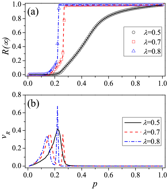
Figure 5: (Color online) Effects of the fraction of activists on binary spreading threshold model. (a) $R(\infty)$ and (b) $v_{R}$ as a function of $p$ for different $\lambda$. In figure (a), symbols represent the simulated results, and the lines are the theoretical predictions from Eqs. (12)-(14) and (16)-(20). Lines in (b) are the simulation results of $v_{R}$. We set other parameters to be $N=10,000$ and $T_{b}=4$.

From the above analysis, it can be obtained that both $\lambda$ and $p$ markedly affect $R(\infty)$ and phase transition. Thus, we further investigate $R(\infty)$ and phase transition on parameter plane $(\lambda,p)$ when $T_{b}=4$ in Fig. 6. Obviously, $R(\infty)$ increases with $\lambda$ and $p$. According to the type of phase transition, the parameter plane $(\lambda,p)$ is divided into four different regions by three vertical lines. The first vertical line can be gotten from Eq. (25), and the other two can be predicted by solving Eqs. (21), (26) and (30). In region I ($p\leq p_{c}^{\star}=1/9$), there are a few activists, who can not percolate the entire population. Thus, no matter what the value of $\lambda$, activists can not be made to adopt the behavior globally. When $p>p_{c}^{\star}$, the global behavior adoption becomes possible, and a crossover phenomenon, which means that the phase transition changes from being hybrid to being second-order, occurs in the phase transition. Meanwhile, the local and global behavior adoptions are separated by the red solid curve (i.e., $\lambda_{c}^{II}$). In region II ($1/9<p\leq 0.15$), the relatively few activists lead to the continuous phase transition. In this region, $R(\infty)$ grows continuously versus $\lambda$ for a given $p$, and a finite fraction of individuals adopt the behavior above $\lambda_{c}^{II}$. With the increase of $p$, in region III ($0.15<p<0.5$), the hybrid phase transition occurs, i.e., $R(\infty)$ first grows continuously with $\lambda$ and then follows by a discontinuous pattern. A finite fraction of activists adopt the behavior above $\lambda_{c}^{II}$, and further induce the bigots to adopt the behavior simultaneously above $\lambda_{c}^{I}$ [see black curves obtained from Eq. (26)]. In region IV ($p\geq 0.5$), half of the neighbors of bigots are activists. Once these activists adopt the behavior, the bigots will gradually adopt the behavior. Thus, $R(\infty)$ grows continuously and a finite fraction of individuals adopt the behavior above $\lambda_{c}^{II}$ (see red curves). Our theoretical predictions of $\lambda_{c}^{II}$, $\lambda_{c}^{I}$ and $R(\infty)$ have a good agreement with the numerical predictions.

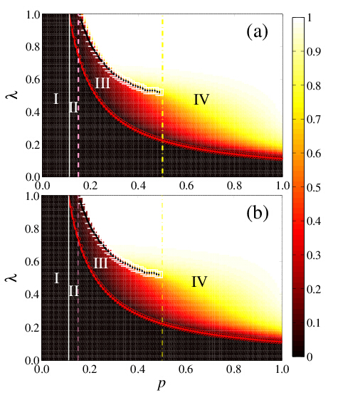
Figure 6: (Color online) Dependence of $R(\infty)$ on $p$ and $\lambda$ on random regular networks. Color-coded values $R(\infty)$ are obtained from numerical simulations (a) and theoretical solutions (b) in the parameter plane $(p,\lambda)$, and the theoretical predictions are the solutions of Eqs. (12)-(14) and (16)-(20). The plane are divided into four regions by three vertical lines, of which the first line can be gotten from Eq. (25) and the other two are predicted by solving Eqs. (21), (26) and (30). In region I, only a vanishingly small fraction of individuals can be exposed to adopt the behavior (i.e., local behavior adoption). Both the regions II and IV show a continuous phase transition, while region III exhibits a hybrid phase transition. The red circles (red solid curve) and white squares (black dished curve) are the continuous and discontinuous simulated (theoretical) critical information transmission probability, respectively. Moreover, other parameters defined as $N=10,000$, $p=0.3$ and $T_{b}=4$.

It can be seen in Fig. 3 that $R(\infty)$ increases discontinuously with $\lambda$ when $T_{b}=2$, thus $R(\infty)$ and phase transition on parameter plane $(p,\lambda)$ for $T_{b}=2$ is explored in Fig. 7. And we find another crossover phenomenon in the phase transition: a change from being first-order to being second-order. Similar to Fig. 6 is that the plane is divided into three regions: Region I ($p\leq 1/9$), the local behavior adoption region, in which only a vanishingly small fraction of individuals adopt the behavior; region II ($1/9<p\leq 0.42$) shows a first-order phase transition, where a finite fraction of individuals adopt the behavior simultaneously above $\lambda_{c}^{I}$ (red dished lines); region III ($p>0.42$) exhibits a second-order phase transition, in which $R(\infty)$ increases continuously versus $\lambda$. The type of phase transition is verified by bifurcation analysis and studying $v_{R}$.

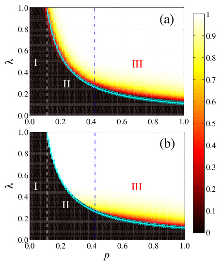
Figure 7: (Color online) Dependence of $R(\infty)$ on $p$ and $\lambda$. Color-coded values $R(\infty)$ from numerical simulations (a) and theoretical solutions (b) in the parameter plane $(p,\lambda)$, and the theoretical predictions are the solutions of Eqs. (12)-(14) and (16)-(20). Two vertical lines separate the plane into three regions, the former line is predicted by Eq. (25) and the latter line is predicted by numerically solving Eqs. (21), (26) and (30). In region I, only a vanishingly small fraction of individuals can be exposed to adopt the behavior (i.e., local behavior adoption). Region II shows a discontinuous phase transition, while region III exhibits a continuous phase transition. The blue circles (blue dished solid curve) are the simulated (theoretical) critical information transmission probability, respectively. We set other parameters as $N=10,000$, $p=0.3$ and $T_{b}=2$.

IV.2 Heterogeneous networks

We turn to elucidate the effects of network heterogeneity. To build the heterogeneous networks, the uncorrelated configuration model with power-law degree distributions $P(k)\sim k^{-\gamma_{D}}$ is adopted, where the mean degree $\langle k\rangle=10$ and the maximum degree $k_{max}\sim\sqrt{N}$ Catanzaro2005 . The network heterogeneity increases with the decrease of $\gamma_{D}$.

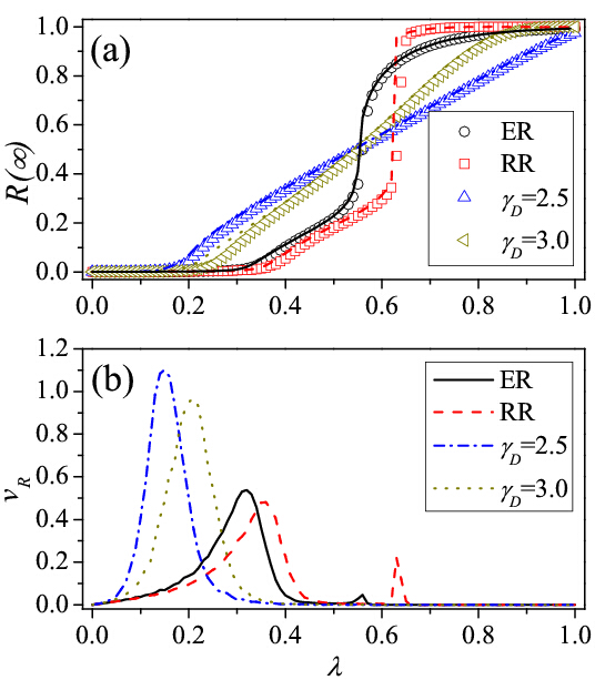
Figure 8: (Color online) For $T_{b}=4$, the effects of network heterogeneity on binary spreading threshold model. (a) $R(\infty)$ and (b) $v_{R}$ versus $\lambda$ on random regular networks, Erdős-Rényi (ER) networks, and scale-free networks with degree exponent $\gamma_{D}=2.5$ and $3.0$. In figure (a), symbols represent the simulated results, and the lines are theoretical predictions from Eqs. (12)-(14) and (16)-(20). Lines in (b) are the simulation results of $v_{R}$. We set other parameters to be $N=10,000$ and $p=0.3$.

In the case of $T_{b}=4$, we find that the global behavior adoption more likely to occur (i.e., lower $\lambda_{c}^{II}$) in heterogeneous networks, due to the existence of hubs in heterogeneous networks Holme2003 , as shown in Fig. 8. Meanwhile, in strong heterogeneous networks a large number of individuals with small degrees are difficult to adopt the behavior, so $R(\infty)$ is smaller at large $\lambda$. For example, $R(\infty)$ at $\lambda=0.7$ is obversely smaller on scale-free networks with $\gamma_{D}=2.5$ than that on RRNs. By bifurcation analysis of Eq. (21), it is discovered that the hybrid phase transition disappears for strong heterogeneous networks (e.g., $\gamma_{D}=2.5$ and $3.0$ in Fig. 8). That is to say, network heterogeneity leads to the crossover phenomenon: a change from being hybrid to being second-order. Moreover, the type of phase transition transition is further verified by observing $v_{R}$ in Fig. 8(b). Evidences in terms of the quantities $R(\infty)$, $\lambda_{c}^{I}$ and $\lambda_{c}^{II}$ support our edge-based compartmental theory.

For the case of $T_{b}=2$ (see Fig. 9), we find the similar phenomenon of $R(\infty)$: $R(\infty)$ increases (decreases) with network heterogeneity for small (large) $\lambda$. However, the system has the first-order phase transition, which denotes that network heterogeneity does not alter the phase transition. Based on the bifurcation theory and the study of $v_{R}$, the phase transition is verified [see Fig. 9(b)].

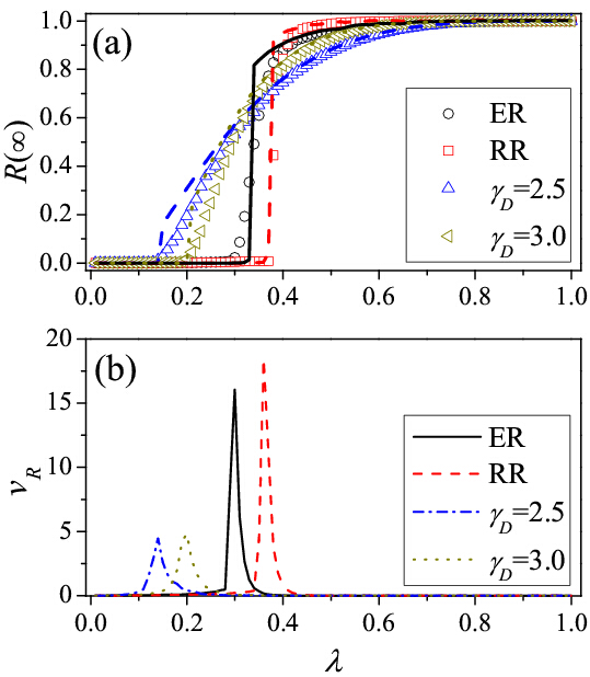
Figure 9: (Color online) For $T_{b}=2$, the effects of network heterogeneity on binary spreading threshold model. (a) $R(\infty)$ and (b) $v_{R}$ versus $\lambda$ on random regular networks, Erdős-Rényi (ER) networks, and scale-free networks with degree exponent $\gamma_{D}=2.5$ and $3.0$. In figure (a), symbols represent the simulated results, and the lines are the theoretical predictions from Eqs. (12)-(14) and (16)-(20). Lines in (b) are the simulation results of $v_{R}$. And other parameters are set to be $N=10,000$ and $p=0.3$.

V Conclusions

Understanding social contagion dynamics in human populations is extremely challenging. In practical behavior spreading, individuals usually display different criterions (wills) to adopt the behavior. That is to say, the heterogeneity of adoption thresholds do indeed exist, but its effects on social contagions have not been verified straightforward. To fill this gap, we proposed a non-Markovian behavior spreading model, in which individuals have distinct adoption thresholds, to explore how heterogeneous adoption thresholds affect the final adoption size and phase transition. An edge-based compartmental theory is developed to quantificationally describe this model, and this suggested theory is verified by a large number of simulations. In the paper, we mainly focused on the so-called binary spreading threshold model, in which a fraction of individuals $p$ have the adoption threshold $T_{a}=1$ and are acted as activists, and the remaining ones have a higher adoption threshold $T_{b}$ and are regarded as bigots.

We first studied the spreading dynamics on random regular networks. And it is found that heterogeneous adoption thresholds markedly affect $R(\infty)$, and induce a hierarchical character in behavior adoption. In other words, activists first adopt the behavior and then stimulate bigots to adopt the behavior. All the first-order, second-order and hybrid phase transitions are found to be in existence in the system. For the case of $T_{b}=1$, the traditional second-order phase transition can be found. For $T_{b}\geq 3$, the hybrid phase transition mixed first and second order, i.e., $R(\infty)$ versus $\lambda$ first grows continuously and then follows by a discontinuous pattern, also occurs. More specifically, the continuous and discontinuous growth of $R(\infty)$ are caused by the activists and bigots, respectively. There is a crossover phenomenon between the hybrid and second-order phase transitions by varying $p$. When $T_{b}=2$, the system only exhibits the first-order or second-order phase transitions. Interestingly, there is another crossover phenomenon: by varying $p$ the phase transition changes from being first-order to being second-order.

Finally, we found that network heterogeneity markedly affects $R(\infty)$ and phase transition due to the existence of hub individuals. For the case of $T_{b}\geq 3$, strong network heterogeneity causes the phase transition to change from being hybrid to being second-order. For $T_{b}=2$, network heterogeneity does not alter the type of phase transition.

The main contribution of our work lies in providing a qualitative and quantitative view on the influence of heterogeneous adoption threshold. Meanwhile, our research results also enrich the phase transition phenomenon. The developed theory can be generalized to behavior spreading with general adoption threshold distribution, and offer some new inspirations for other similar spreading dynamics, such as epidemic spreading and cascading. However, some fascinating and hopeful challenges still remain. For example, what will happen if the adoption thresholds are correlated with their degrees? How to extract more realistic behavior spreading mechanisms from real data?

References

References

- (1) Watts D J and Dodds P S 2007 Journal of Consumer Research, 34 441.
- (2) Castellano C, Fortunato S and Fortunato S 2009 Rev. Mod. Phys. 81 0034.
- (3) Christakis N A and Fowler J H 2007 N. Engl. J. Med. 357 370.
- (4) Barrat A, Barthélemy M, and Vespignani A 2007 Dynamical Processes on Complex Networks (Cambridge: Cambridge University Press).
- (5) Centola D 2011 Science 334 1269.
- (6) Banerjee A, Chandrasekhar A G, Duflo E and Jackson M O 2013 Science 341 363.
- (7) Pastor-Satorras R, Castellano C, Mieghem P V and Vespignani A 2014 arXiv:1408.2701v1.
- (8) Moreno Y, Pastor-Satorras R and Vespignani A 2002 Eur. Phys. J. B 26 521.
- (9) Pastor-Satorras R and Vespignani A 2001 Phys. Rev. Lett. 86 3200.
- (10) Salathé M and Khandelwal S 2011 PLOS Comput. Biol. 7 e1002199.
- (11) Yang H X, Tang M, and Lai Y C 2015 Phys. Rev. E 91 062817.
- (12) Yang H X , Wang W X, Lai Y C, Xie Y B, and Wang B H 2011 Phys. Rev. E 84 045101(R).
- (13) Li K, Fu X, Small M, and Zhu G 2014 Chaos 24 043124.
- (14) Porter M A and Gleeson J P 2014 arXiv:1403.7663v1.
- (15) Watts D J 2002 Proc. Natl. Acad. Sci. 99 5766.
- (16) Granovetter M 1973 Am. J. Sociol. 78 1360.
- (17) Gleeson J P and Cahalane D J 2007 Phys. Rev. E 75 056103.
- (18) Singh P, Sreenivasan S, Szymanski B K and Korniss G 2013 Sci. Rep. 3 2330.
- (19) Dodds P S and Payne J L 2009 Phys. Rev. E 79 066115.
- (20) Whitney D E 2010 Phys. Rev. E 82 066110.
- (21) Gleeson J P 2008 Phys. Rev. E 77 046117.
- (22) Nematzadeh A, Ferrara E, Flammini A and Ahn Y Y 2014 Phys. Rev. Lett. 113 088701.
- (23) Brummitt C D, Lee K -M and Goh K-I 2012 Phys. Rev. E 85 045102(R).
- (24) Yaǧan O and Gligor V 2013 Phys. Rev. E 86 036103.
- (25) Dodds P S and Watts D J 2004. Phy. Rev. Lett. 92 218701.
- (26) Wang W, Tang M, Zhang H-F and Lai Y-C 2015 Phys. Rev. E 92 012820.
- (27) Zheng M, Lü L and Zhao M 2013 Phys. Rev. E 88 012818.
- (28) Centola D 2010 Science 329 1194.
- (29) Miller J C 2007 Phys. Rev. E 76 010101.
- (30) Yang H, Tang M and Gross T 2015 Sci. Rep. 5 13122.
- (31) Cui A-X, Wang W, Tang M, Fu Y, Liang X and Do Y 2014 Chaos 24 033113.
- (32) Jo H H, Perotti J I, Kaski K and Kertész J 2014 Phys. Rev. X 4 011041.
- (33) Wu C, Ji S, Zhang R, Chen L, Chen J, Li X and Hu Y 2014 Europhys. Lett. 107, 48001.
- (34) Hu Y, Ksherim B, Cohen R and Havlin S 2011 Phys. Rev. E 84, 066116.
- (35) Cellai D, Lawlor A, Dawson K A and Gleeson J P 2011 Phys. Rev. Lett. 107 175703.
- (36) Baxter G J, Dorogovtsev S N, Goltsev A V and Mendes J F F 2011 Phys. Rev. E 83 051134.
- (37) Lee K-M, Brummitt C D and Goh K-I 2014 Phys. Rev. E 90 062816.
- (38) Karsai M, Iñiguez G, Kaski K and Kertész J 2014 J. R. Soc. Interface 11 101.
- (39) Catanzaro M, Boguñá M and Pastor-Satorras R 2005 Phys. Rev. E 71 027103.
- (40) Wang W, Shu P-P, Zhu Y-X, Tang M and Zhang Y-C 2015 Chaos 25 103102.
- (41) Miller J C, Slim A C and Volz E M 2011 J. R. Soc. Interface. 10 1098.
- (42) Miller J C and Volz E M 2013 PLoS ONE 8 e69162.
- (43) Wang W, Tang M, Zhang H-F, Gao H, Do Y and Liu Z-H 2014 Phys. Rev. E 90 042803.
- (44) Karrer B and Newman M E J 2010 Phys. Rev. E 82 016101.
- (45) Newman M E J, Strogatz S H and Watts D J 2001 Phys. Rev. E 64 026118.
- (46) Strogatz S H 1994 Nonlinear dynamics and chaos: with applications to physics, biology, chemistry and engineering (Westview, Boulder, CO).
- (47) Dorogovtsev S N, Goltsev A V, and Mendes J F F 2008 Rev. Mod. Phys. 80 1275.
- (48) Chen W, Schröder M, D’Souza M R 2014 Phys. Rev. Lett. 112 155701.
- (49) Radicchi F 2015 Phys. Rev. E 91 010801(R).
- (50) Ferreira S C, Castellano C and Pastor-Satorras R 2015 Phys. Rev. E 86 041125.
- (51) Shu P, Wang W and Tang M 2015 Chaos 25 063104.
- (52) Holme P, Kim B J, Yoon C N, and Han S K. 2002 Phys. Rev. E 65 056109.