Fractionalized Fermi liquid
on the surface of a topological Kondo insulator

Abstract

We argue that topological Kondo insulators can also have ‘intrinsic’ topological order associated with fractionalized excitations on their surfaces. The hydridization between the local moments and conduction electrons can weaken near the surface, and this enables the local moments to form spin liquids. This co-exists with the conduction electron surface states, realizing a surface fractionalized Fermi liquid. We present mean-field solutions of a Kondo-Heisenberg model which display such surfaces.

I Introduction

An important development of the past decade has been the prediction and discovery of topological insulators (TI) Hasan and Kane (2010); Qi and Zhang (2011); Kane and Mele (2005); Bernevig et al. (2006); Moore and Balents (2007); Fu et al. (2007); Roy (2009). These materials are well-described by traditional band theory, but possess strong spin-orbit interactions that result in a non-trivial winding of the ground state wavefunction in a manner analogous to the integer quantum Hall effect. Since their discovery, the multitudinous effects of interactions have been a prominent topic of study. One compelling proposal to emerge is the notion of a topological Kondo insulator (TKI) Dzero et al. (2010, 2012, 2015). In contrast to a band insulator, a Kondo insulator only develops an insulating gap at low temperatures, and the magnitude of the gap is controlled by electron-electron interactions. Doniach explained this phenomenon through the Kondo lattice model Doniach (1977) in which a lattice of localized moments is immersed within a sea of conduction electrons. At high temperatures, RKKY-type exchange interactions dominate and an ordered magnetic state results. Conversely, at low energies, strong interactions between localized moments and conduction electrons become important; the system crosses over into either a metallic phase well-described by Fermi liquid theory (FL) or, if the chemical potential is appropriately tuned, a Kondo insulator. As strong spin-orbit coupling is often present in these materials, the possibility that a Kondo insulator may have a nontrivial topological character is well-justified.

Of specific interest has been the Kondo insulator samarium hexaboride (SmB₆). A number of experiments have examined the proposal that it is a TKI: transport measurements have established the presence of metallic surface states Wolgast et al. (2013); Kim et al. (2012); Zhang et al. (2013); Phelan et al. (2014); Kim et al. (2013), and angle-resolved photoemission spectroscopy (ARPES) results appear consistent with the expected Dirac surface cones Neupane et al. (2013); Jiang et al. (2013a); Xu et al. (2013); Denlinger et al. (2014); Jiang et al. (2013b). Nonetheless, the spin-polarized ARPES measurements Jiang et al. (2013b) remain controversial.

However, as the TKI phase is well-described within a mean field framework Dzero et al. (2015), its topological properties are not expected to be markedly different from what has already been observed in its uncorrelated cousins. More intriguing is the potential the topologically protected surface states present for new interesting phases Roy et al. (2014); Nikolić (2014); Alexandrov et al. (2015); Iaconis and Balents (2015). In SmB₆, this expectation is motivated experimentally by ARPES measurements which find light surface quasiparticles Neupane et al. (2013); Xu et al. (2013); Jiang et al. (2013a) in contradiction to current theories which predict heavy particles at the surface Dzero et al. (2010, 2012); Alexandrov et al. (2013); Lu et al. (2013). Ref. Alexandrov et al. (2015) proposes “Kondo breakdown” at the surface as an explanation. They show that the reduced coordination number of the localized moments at the surface may lead to a suppressed Kondo temperature. At low temperature these moments are thermally decoupled from the bulk.

In this paper, we propose the existence of a fractionalized Fermi liquid (SFL^∗) on the surface of a TKI. This state is characterized by “intrinsic topological order” on the surface of a TKI, in which the local moments form a spin liquid state which has ‘fractionalized’ excitations with quantum numbers which cannot be obtained by combining those of one or more electrons Balents (2010). Rather than being thermally liberated, as in Ref. Alexandrov et al., 2015, the surface local moments exploit their mutual exchange interactions to decouple from the conduction electrons, and form a spin liquid state, as in the fractionalized Fermi liquid state (FL^∗) Senthil et al. (2003, 2004). We will present mean-field computations on a Kondo-Heisenberg lattice model which demonstrate the formation of mutual singlets between the surface local moments, while conducting surface states of light electronic quasiparticles are also present.

Somewhat confusingly, our SFL^∗ state is ‘topological’ in two senses of the word, a consequence of unfortunate choices (from our perspective) in the conventional terminology. As in conventional TI, it is ‘topological’ because it has gapless electronic states on the surface induced by the nature of the bulk band structure. However, it is also ‘topological’ in the sense of spin liquids Balents (2010), because of the presence of fractionalized excitations among the local moments on the surface.

The outline of our paper is as follows. We specify our Kondo-Heisenberg model in Section II. In Section III, we present the mean-field solution of this model for the case of a translationally-invariant square lattice with periodic boundary conditions. The effect of the surface on the mean field solutions is addressed in Section IV where the presence of the SFL^∗ state is numerically demonstrated. We conclude in Section V with a discussion of our results and their relevance to physical systems.

II Model

Here we present the specific form of the Kondo-Heisenberg lattice model to be studied:

$$H=H_{c}+H_{H}+H_{K}\,.$$ (1)

The first terms represents the hopping Hamiltonian of the conduction electrons,

$$H_{c} =-\sum_{\braket{ij}}t_{ij}\left(c_{i\alpha}^{\dagger}c_{j\alpha}+h.c.\right)\,,$$ (2)

where the operator $c_{i\alpha}^{\dagger}$ creates an electron at site ${\mathbf{r}}_{i}$ of spin $\alpha=\uparrow,\downarrow$. The remaining two terms establish the form of the interactions: $H_{H}$ is a generalized Heisenberg term which specifies the inter-spin interaction while $H_{K}$ is a Kondo term and describes the electron-spin exchange.

The spin-orbit coupling of the $f$-orbital imposes a classification in terms of a $(2J+1)$ multiplet, where $J$ is the total angular momentum. In general, this degeneracy is further lifted by crystal fields and we will consider the simplest case of a Kramers degenerate pair of states. We start from an Anderson lattice model Anderson (1961) with hopping $t_{f}$ between $f$-orbitals and onsite repulsion $U_{f}$. To access the Kondo limit ($U_{f}\rightarrow\infty$), we perform a Schrieffer-Wolff transformation Schrieffer and Wolff (1966) and obtain a term of the form

$$H_{H}=-{J_{H}\over 2}\sum_{\braket{ij}}f_{i\alpha}^{\dagger}f_{j\alpha}f_{j\beta}^{\dagger}f_{i\beta}\,,$$ (3)

where $f_{i\alpha}$ creates a spinon at site ${\mathbf{r}}_{i}$, and $J_{H}\sim t^{2}_{f}/U_{f}$. This limit imposes the constraint $\sum_{\alpha}f_{i\alpha}^{\dagger}f_{i\alpha}=1$ and further ensures that the correct commutation relations for the “spin” operators $S^{a}_{j}={1\over 2}f^{\dagger}_{j\alpha}\sigma^{a}_{\alpha\beta}f_{j\beta}$ are obeyed. By using the Fierz identity (and dropping a constant) we can verify that we indeed have the familiar Heisenberg term:

$$H_{H}={J_{H}\over 4}\sum_{\braket{ij}}f_{i\alpha}^{\dagger}\boldsymbol{\sigma}_{\alpha\beta}f_{i\beta}\cdot f_{j\gamma}^{\dagger}\boldsymbol{\sigma}_{\gamma\delta}f_{j\delta}=J_{H}\sum_{\braket{ij}}\mathbf{S}_{i}\cdot\mathbf{S}_{j}\,,$$ (4)

where $\boldsymbol{\sigma}=\left(\sigma^{x},\sigma^{y},\sigma^{z}\right)$. It is important to note that the spinon operators $f_{j\alpha}$ do not have a uniquely defined phase. In fact, by choosing to represent the spins in terms of constrained fermion operators, we are formulating the Kondo lattice model as a U(1) gauge theory. This emergent gauge structure is what permits a realization of the fractionalized phases we will discuss Senthil et al. (2003, 2004).

For the electron-spin interaction, $H_{K}$, we follow the construction of Coqblin-Schrieffer Coqblin and Schrieffer (1969) for systems with spin-orbit coupling. In order for the interaction to transform as a singlet, the electron and spin must couple in a higher angular momentum channel. For simplicity, we assume a square lattice and that the spins and conduction electrons carry total angular momentum differing by $l=1$. In the Anderson model, an appropriate interaction term is then

$$H_{int}\sim\mathcal{V}\sum_{{\mathbf{k}},\alpha}\left(\alpha\sin k_{x}-i\sin k_{y}\right)c_{{\mathbf{k}}\alpha}^{\dagger}\ket{f^{0}}\bra{f^{1};\alpha}+h.c.$$ (5)

For instance, the interaction between moments with total angular momentum $J=3/2$ and spin-1/2 electrons would take this form. We will verify in the next section that for the purpose of obtaining a TKI, this coupling is sufficient. We next define the electron operators

$$d_{{\mathbf{k}}\alpha} =2\left(\alpha\sin k_{x}+i\sin k_{y}\right)c_{{\mathbf{k}}\alpha}, d_{i\alpha} =-i\alpha(c_{i+\mathbf{\hat{x}},\alpha}-c_{i-\mathbf{\hat{x}},\alpha})+(c_{i+\mathbf{\hat{y}},\alpha}-c_{i-\mathbf{\hat{y}},\alpha})\,.$$ (6)

and, taking the same $U_{f}\rightarrow\infty$ limit as above, again implement the Schrieffer-Wolff transformation Schrieffer and Wolff (1966) to obtain

$$H_{K}=-{J_{K}\over 4}\sum_{i}f^{\dagger}_{i\alpha}d_{i\alpha}d_{i\beta}^{\dagger}f_{i\beta}$$ (7)

where $J_{K}\sim\mathcal{V}^{2}/U_{f}$.

We next perform a Hubbard-Stratonovich transformation of the Kondo and Heisenberg terms:

$$H^{\prime}= H_{1}+H_{0}$$

$$H_{1}= -\sum_{\braket{ij}}\left((t_{ij}-\delta_{ij}\mu_{i})c_{i\alpha}^{\dagger}c_{j\alpha}+h.c.\right)+{1\over 2}\sum_{j\alpha}\left[V_{j}f_{j\alpha}^{\dagger}d_{j\alpha}+V_{j}^{*}d_{j\alpha}^{\dagger}f_{j\alpha}\right]$$

$$-{1\over 2}\sum_{j\alpha\boldsymbol{\hat{\mu}}}\left[\chi_{j\mu}f_{j+\boldsymbol{\hat{\mu}},\alpha}^{\dagger}f_{j\alpha}+\chi^{*}_{j\mu}f_{j\alpha}^{\dagger}f_{j+\boldsymbol{\hat{\mu}},\alpha}\right]+\sum_{j}\lambda_{j}f_{j\alpha}^{\dagger}f_{j\alpha}$$

$$H_{0}= \sum_{j}\left[-\lambda_{j}+{\left|V_{j}\right|^{2}\over J_{K}}+\sum_{\boldsymbol{\hat{\mu}}}{\left|\chi_{j\mu}\right|^{2}\over 2J_{H}}\right]\,.$$ (8)

We proceed with a saddle-point approximation, and treat the fields $V_{j}$, $\chi_{j\mu}$, and $\lambda_{j}$ as real constants subject to the self-consistency conditions

$$V_{j} =-{J_{K}\over 2}\Braket{d_{j\alpha}^{\dagger}f_{j\alpha}}, \chi_{j\mu} ={J_{H}}\Braket{f_{j\alpha}^{\dagger}f_{j+\boldsymbol{\hat{\mu}},\alpha}}\,,$$ (9)

$$1 =\Braket{f_{j\alpha}^{\dagger}f_{j\alpha}}\,.$$ (10)

This can be formally justified within a large-$N$ expansion of Eq. 1, with $N$ the number of spinons. As we are specifying to the case of an insulator, it further makes sense to require perfect half-filling. Since $n_{f}=1$ already, this results in a final equation for the chemical potential $\mu_{j}$:

$$1 =\Braket{c_{j\alpha}^{\dagger}c_{j\alpha}}\,.$$ (11)

III Translationally invariant system

We begin by solving Eqs. 9$\,-\,$11 in a translationally invariant system with periodic boundary conditions on a square lattice. Letting $V_{j}=V$, $\chi_{jx}=\chi_{jy}=\chi$, $\lambda_{j}=\lambda$ and $\mu_{j}=\mu$, we perform a Fourier transform:

$$H_{1} =\sum_{\mathbf{k}}\Psi_{\mathbf{k}}^{\dagger}\mathcal{H}({\mathbf{k}})\Psi_{\mathbf{k}}\qquad\qquad \Psi^{\dagger}_{\mathbf{k}} =\left(c_{{\mathbf{k}}\uparrow}^{\dagger},f_{{\mathbf{k}}\uparrow}^{\dagger},c_{{\mathbf{k}}\downarrow}^{\dagger},f_{{\mathbf{k}}\downarrow}^{\dagger}\right)$$ (12)

$$\mathcal{H}({\mathbf{k}}) =\begin{pmatrix}h({\mathbf{k}})&0\\ 0&h^{*}(-{\mathbf{k}})\end{pmatrix} h({\mathbf{k}}) =\begin{pmatrix}\epsilon_{c}({\mathbf{k}})&V(\sin k_{x}+i\sin k_{y})\\ V(\sin k_{x}-i\sin k_{y})&\epsilon_{f}({\mathbf{k}})\\ \end{pmatrix}\,.$$ (13)

For simplicity, we only consider nearest-neighbour coupling between spins; for the electron dispersion, a slightly more general description is required and we also take next-nearest neighbour hopping into account. The dispersions are given by

$$\epsilon_{c}({\mathbf{k}}) =-t_{1}(\cos k_{x}+\cos k_{y})-2t_{2}\cos k_{x}\cos k_{y}-\mu, \epsilon_{f}({\mathbf{k}}) =-\chi(\cos k_{x}+\cos k_{y})+\lambda$$ (14)

where the subscripts “$c$” and “$f$” refer to the electrons and spinons respectively. In the following, we will use units of energy where $t_{1}=1.0$.

Since TI’s exist as a result of a band inversion, it’s important to ask which sign $\chi$ will take. Naturally, when $V=0$, the particle-hole symmetry of our mean field ansatz implies that $\chi>0$ and $\chi<0$ have the same energy. At finite hybridization, however, one will become preferable. We note that when $\chi$ and $t_{1}$ have opposite signs, the energy of the lower band will be less than the Fermi energy and hence occupied throughout most of the Brillouin zone (BZ): an increase in $V$ will push most of these states to lower energies. Conversely, if $\chi$ and $t_{1}$ take the same sign, in one of part of the BZ no states will lie below the Fermi energy while in another both the upper and lower band will. It therefore makes sense to expect $\text{sign}\left(\chi\right)=-\text{sign}\left(t_{1}\right)$. In the parameter regime explored, the numerics always find this to be the case.

By construction, the Hamiltonian $H_{1}$ supports a non-trivial topological phase and is in fact the familiar Bernevig-Zhang-Hughes model Bernevig et al. (2006) used to describe the quantum spin Hall effect in HgTe wells. We can see this by studying the eigenfunctions of $h({\mathbf{k}})$:

$$\psi_{\pm}({\mathbf{k}})={1\over\sqrt{2d(d\pm d_{3})}}\begin{pmatrix}d_{3}\pm d\\ V(\sin k_{x}+i\sin k_{y})\end{pmatrix}$$ (15)

where $d({\mathbf{k}})=\sqrt{d_{3}({\mathbf{k}})^{2}+V^{2}(\sin^{2}k_{x}+\sin^{2}k_{y})}$, and $d_{3}({\mathbf{k}})=\left(\epsilon_{c}({\mathbf{k}})-\epsilon_{f}({\mathbf{k}})\right)/2$. If $d_{3}({\mathbf{k}})>0$ or $d_{3}({\mathbf{k}})<0$ for all ${\mathbf{k}}$, these functions are well-defined on the entire BZ and the system is in a topologically trivial phase Bernevig and Hughes (2013). If this is not the case then it is impossible to choose a globally defined phase – the ground state wavefunction has nontrivial winding and characterizes a topological insulator. From Eq. 14, we see that this occurs when

$$-2<{\mu+\lambda+2t_{2}\over t_{1}-\chi}<2\,.$$ (16)

Alternatively, we can obtain the same result by calculating the $\mathds{Z}_{2}$ invariant $\nu$ Fu and Kane (2007): when Eq. 16 holds, $\nu=-1$ and the system is a TI.

We will typically be studying systems with $\left|t_{1}\right|\gg\left|\chi\right|$ and $\left|t_{2}/t_{1}\right|$ small (implying $\mu$ and $\lambda$ small as well), so Eq. 16 is not difficult to fulfill. In Fig. 1 the energy spectrum of the system in a slab geometry is shown for $J_{H}=0.15$, $J_{K}=0.3$. Half-filling is maintained on every site (see Appendix A), but $V$ and $\chi$ were determined by self-consistently solving Eq. 9 in a periodic system. In Fig. 1(b), the topologically protected Dirac cone is clearly visible.

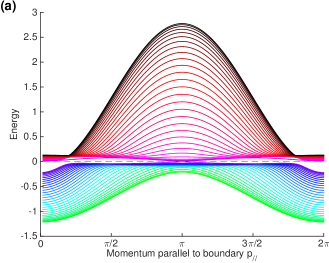
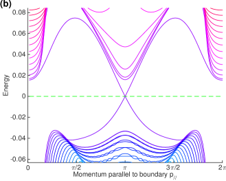
Figure 1: Energy spectrum for $J_{H}=0.15$, $J_{K}=0.3$. Both $V$ and $\chi$ are constant throughout the bulk, but both $\mu_{i}$ and $\lambda_{i}$ have been self-consistently solved to ensure that $n_{c}=n_{f}=1$ on every site (see Appendix A). (a) The full spectrum is shown. (b) A closer view of the insulating gap, where the Dirac cone is clearly visible. We use units with $t_{1}=1.0$. Calculations were done with $t_{2}=-0.25$ and at a temperature of $10^{-5}$.

If we ignore the effect the boundary will have on the values of $V$, $\chi$, and $\lambda$, we can calculate the Fermi velocity of the Dirac cone Bernevig and Hughes (2013):

$$v_{F}=2V\sqrt{\frac{\left|\chi(t_{1}-2t_{2})\right|}{\left|t_{1}-2t_{2}\right|+\left|\chi\right|}}\sim 2V\sqrt{\left|\chi\right|}$$ (17)

where we’ve assumed $\left|\chi\right|\ll t_{1}$ in the second equation. This is consistent with the prediction that the quasiparticles at the surface be heavy Dzero et al. (2010, 2012); Alexandrov et al. (2013); Lu et al. (2013). For the parameters shown in Fig. 1, this formula predicts $v_{F}=0.0592$, consistent with the numerically determined value $v_{F}=0.0585$.

IV System with boundary

We now consider the effect the boundary will have on the mean field configuration and demonstrate the presence of two new fractionalized phases. Generally, we expect that the lower coordination number at the boundary will suppress the (nonlocal) hybridization: $V_{\rm surf}\sim 3V_{\rm bulk}/4$. While the decrease in $V_{\rm surf}$ will induce an increase in the spinon bond parameter $\chi_{i\mu}$ Paul et al. (2008) both parallel and perpendicular to the surface, the parameter parallel to the surface will be more strongly affected. Since Heisenberg coupling ultimately favours an alternating bond order, in the absence of hybridization $V$, this anisotropy will result in a further decrease in the magnitude of the spinon bond parameter perpendicular to the surface, $\left|\chi_{\perp}\right|$.

When these effects are predominant, an FL^∗ on the surface is realized: the hybridization $V_{i}$ vanishes on one or more layers at the surface and $\chi_{\perp}$ vanishes on the innermost layer. The existence of the SFL^∗ phase is shown numerically by self-consistently solving Eqs. 9$-$11 in a slab geometry and comparing ground states energies (some details are given in Appendix A). The resulting phase diagram is shown in Fig. 2(a). In fact, we find two distinct SFL^∗ phases: a decoupled spin chain and a decoupled spin ladder, which are depicted in Figs. 2(b) and 2(c) respectively. In Fig. 3 we plot the spatial dependence of the mean field parameters in both SFL^∗ states. The plots in the left column correspond to a spin chain SFL^∗ state whereas the right column corresponds to a spin ladder SLF^∗ state. The phases are distinguished by whether $V$ vanishes on the first site only or on both the first and second site, shown in Fig. 3(a) and (b) respectively. In Figs. 3(c) and (d) our intuition regarding the behaviour of $\chi$ near the boundary is confirmed: $\left|\chi_{\perp}\right|$ is suppressed to zero whereas $\left|\chi_{\parallel}\right|$ increases to the value it would assume in a single dimension. The fluctuations of the Lagrange multiplier field $\lambda$ (Figs. 3(e) and (f)) are a reflection of the on-site requirement of half-filling for both the spinons and electons.

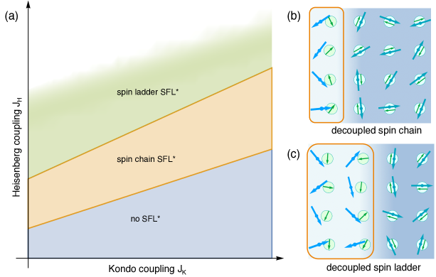
Figure 2: (a) Schematic phase diagram of surface states. (b),(c) Cartoon depictions of surface FL^∗ states. In the dark blue region, the electron spins and localized moments are locked into singlets. Towards the edge (the pale blue region outlined in orange) the conduction electrons decouple from the moments, and the latter form a spin liquid. Naturally, the conduction electrons remain coupled to each other at all sites.

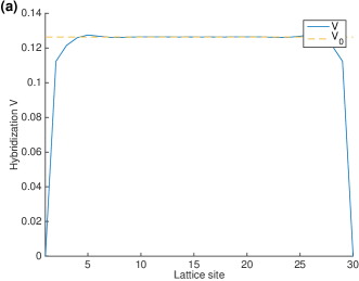
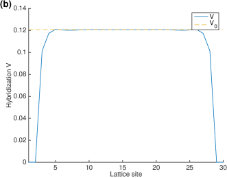
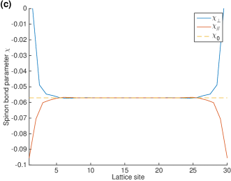
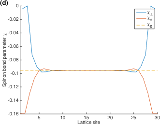
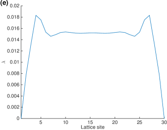
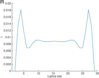
Figure 3: Spatial dependence of mean field parameters in SFL^∗ phases. In the left column, we plot values corresponding to the spin chain SFL^∗ ($J_{H}=0.15$, $J_{K}=0.3$) while on the right values corresponding to the spin ladder SFL^∗ ($J_{H}=0.25$, $J_{K}=0.3$) are shown. (a),(b) Hybridization $V_{i}$. (c),(d) Spinon bond parameters $\chi_{i\mu}$ in the direction perpendicular (blue) and parallel (red) to the boundary. (e),(f) The Lagrange multiplier field $\lambda_{i}$. In (a)$-$(f), the yellow dashed line plots the value obtained in the translationally invariant case. We use units with $t_{1}=1.0$. Calculations were done with $t_{2}=-0.25$ and at a temperature of $10^{-5}$.

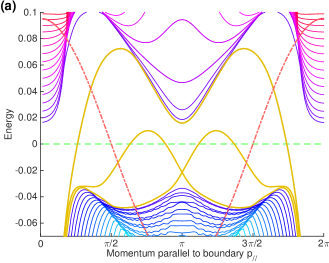
Figure 4: Energy spectra in SFL^∗ phases. (a) Spin chain SFL^∗ ($J_{H}=0.15$, $J_{K}=0.3$). The ground state has $V_{i}=0$ on the first surface layer and the moments form a spin chain decoupled from the bulk. (b) Spin ladder SFL^∗ ($J_{H}=0.25$, $J_{K}=0.3$). The ground state has $V_{i}=0$ on the first two layers and a spin ladder is present on the surface. In both figures, the dash-dotted red curve represents the one-dimensional cosine dispersion found for the spinons and is merely an artifact of the ansatz. We use units with $t_{1}=1.0$. Calculations were done with $t_{2}=-0.25$ and at a temperature of $10^{-5}$.

In Fig. 4(a), the spectrum of the spin chain SFL^∗ state is shown. The red dash-dotted curve is the dispersion of the spinons calculated at mean field. While we do not claim that this accurately represents the Heisenberg chain, we nonetheless expect gapless spin excitations Haldane (1988). The remaining in-gap states can be understood as the result of the mixing of the surface layer of conduction electron with the Dirac cone. Consistent with its topology, even if the Dirac cone is no longer present at the chemical potential, two chiral bands traverse the gap from the conduction to the valence band and the surface is metallic. In this case, an additional four metallic surface states per spin are present, but these are not topologically protected and we can imagine pushing them below the chemical potential in a number of ways, such as, for instance, softening the restriction imposed by Eq. 11.

The spectrum corresponding to the second surface FL^∗ state, the decoupled spin ladder, is shown in Fig. 4(b). The red curve representing the spinons is now two-fold degenerate per spin (a small splitting is hidden by the thickness of the line). Even more so than for the spin chain, this result is an artifact of the mean field calculations: save in the limit where the legs of the ladder are completely decoupled, a ladder of spin-1/2 particles is gapped Haldane (1988); Giamarchi (2003).

In both phases, the metallic bands have lighter quasiparticles than predicted by the translationally invariant theory in Eq. 17. For the spin chain, the surface velocity of the leftmost state in Fig. 4(a) is $v_{F}=0.095$, compared to $v_{F}=0.052$ for the Dirac cone of Fig. 1(b). For the spin ladder, the effect is even more pronounced. There, the lightest state has a Fermi velocity of $v_{F}=0.48$ compared to the translationally-invariant value $v_{F}=0.072$.

The structure of the fractionalized excitations in the SFL^∗ states found here is rather simple: just a free gas of neutral $S=1/2$ spinon excitations. We view this mainly as a ‘proof of principle’ that such SFL^∗ states can exist on the surface of TKI. Clearly, more complex types of spin liquid states are possible on the surface, and also in three-dimensional TKI with two-dimensional surfaces.

V Discussion

The strong electron-electron interactions in topological Kondo insulators make them appealing candidates for searching for novel correlated electron states. In many heavy-fermion compounds, the strong interactions acting on the $f$-electron local moments are quenched by the Kondo screening of the conductions electrons, and the resulting state is eventually a Fermi liquid, or a band insulator for suitable density. The topological Kondo insulators offer the attractive possibility that the hybridization between the local moments and the conduction electron states can be weakened near the surface Roy et al. (2014); Alexandrov et al. (2015), and this could explain the light effective masses associated with the surface electronic states Neupane et al. (2013); Xu et al. (2013); Jiang et al. (2013a). With the weakened hybridization, we have proposed here that the local moments may form a spin liquid state with ‘intrinsic’ topological order. As the fractionalized excitations of such a spin liquid co-exist with the conduction electron surface states similar to those of a conventional TI, the surface realizes a fractionalized Fermi liquid Senthil et al. (2003, 2004).

This paper has presented mean-field solutions of Kondo-Heisenberg model on a square lattice which act as a proof-of-principle of the enhanced stability of the such surface fractionalized Fermi liquids (SFL^∗). We fully expect that such solutions also exist on the surfaces of three-dimensional lattices, relevant to a Kondo insulator like SmB₆.

The recent evidence for bulk quantum oscillations in insulating SmB₆ Tan et al. (2015) is exciting evidence for the non-trivial many-electron nature of these materials. It has been proposed Knolle and Cooper (2015) that these oscillations appear because the magnetic-field weakens the hybridization between the conduction electrons and the local moments, and this releases the conduction electrons to form Fermi surfaces leading to the quantum oscillations. The fate of the local moments was not discussed in Ref. Knolle and Cooper, 2015, but a natural possibility is that they form a bulk spin liquid, similar to the surface spin liquid we have discussed here. Thus, while we have proposed here the formation of a SLF* states in SmB₆ in zero magnetic field, it may well be that a bulk FL^∗ state forms in high magnetic field.

Appendix A Mean field theory with boundary

In this appendix, we consider the mean field equations in the presence of a boundary. We define the lattice to be finite in the $x$-direction, $x_{i}=1,\ldots,N$, and infinite in the $y$-direction (to remove factors of $i$, we actually switch the $x$- and $y$-directions compared to Eq. 6). We rewrite the Fourier transform, which is now only valid in the $y$-direction:

$$c_{ij\sigma} =\int{dk\over 2\pi}e^{iky_{j}}c_{ik\sigma}, d_{ij\alpha} =\int{dk\over 2\pi}e^{iky_{j}}\left[2\alpha\sin k\,c_{ik\alpha}+(c_{j+1,k\alpha}-c_{i-1,k\alpha})\right],$$

$$f_{ij\sigma} =\int{dk\over 2\pi}e^{iky_{j}}f_{ik\sigma}.$$ (18)

Translational invariance in the $y$-direction implies that the mean field parameters will depend only on the distance from the boundary – the roman indices $i$, $j$, etc. label the $x$-coordinate only. We express the Hamiltonian in block form as

$$\hat{H}_{MF} =\sum_{k}\Psi^{\dagger}_{k\sigma}\mathcal{H}_{\sigma}(k)\Psi_{k\sigma}, \Psi_{k\sigma}^{\dagger} =\left(c_{1k\sigma}^{\dagger},c_{2k\sigma}^{\dagger},\ldots,f_{1k\sigma}^{\dagger},f_{2k\sigma}^{\dagger},\ldots\right)$$

$$=\left(\psi_{1k\sigma}^{\dagger},\psi_{2k\sigma}^{\dagger},\ldots,\psi_{1+N,k\sigma}^{\dagger},\psi_{2+N,k\sigma}^{\dagger},\ldots\right)$$

$$\mathcal{H}_{\uparrow}(k) =\begin{pmatrix}h_{c}(k)&h_{cf}(k)\\ h_{cf}^{\dagger}(k)&h_{f}(k)\end{pmatrix} \mathcal{H}_{\downarrow}(k) =\mathcal{H}_{\uparrow}(-k)^{*}$$ (19)

with blocks given by

$$h_{c}(k) =-{t_{1}\over 2}\begin{pmatrix}2\cos k&1&0&\cdots\\ 1&2\cos k&1&\cdots\\ 0&1&2\cos k&\cdots\\ \vdots&\vdots&\vdots&\ddots\end{pmatrix}-t_{2}\cos k\begin{pmatrix}0&1&0&\cdots\\ 1&0&1&\cdots\\ 0&1&0&\cdots\\ \vdots&\vdots&\vdots&\ddots\end{pmatrix}-\begin{pmatrix}\mu_{1}&0&0&\cdots\\ 0&\mu_{2}&0&\cdots\\ 0&0&\mu_{3}&\cdots\\ \vdots&\vdots&\vdots&\ddots\end{pmatrix}$$ (20)

$$h_{f}(k) =-{1\over 2}\begin{pmatrix}2\chi_{1y}\cos k&\chi_{1x}&0&0&\cdots&\cdots&\cdots\\ \chi_{1x}&2\chi_{2y}\cos k&\chi_{2x}&0&\cdots&\cdots&\cdots\\ 0&\chi_{2x}&2\chi_{3y}\cos k&\chi_{3x}&\cdots&\cdots&\cdots\\ \vdots&\vdots&\vdots&\vdots&\ddots&\cdots&\cdots\\ \vdots&\vdots&\vdots&\vdots&\vdots&2\chi_{N-1,y}\cos k&\chi_{N-1,x}\\ \vdots&\vdots&\vdots&\vdots&\vdots&\chi_{N-1,x}&2\chi_{Ny}\cos k\end{pmatrix}$$

$$\qquad+\begin{pmatrix}\lambda_{1}&0&0&0&\cdots&\cdots&\cdots\\ 0&\lambda_{2}&0&0&\cdots&\cdots&\cdots\\ 0&0&\lambda_{3}&0&\cdots&\cdots&\cdots\\ \vdots&\vdots&\vdots&\vdots&\ddots&\cdots&\cdots\\ \vdots&\vdots&\vdots&\vdots&\vdots&\lambda_{N-1}&0\\ \vdots&\vdots&\vdots&\vdots&\vdots&0&\lambda_{N}\end{pmatrix}$$ (21)

$$h_{cf}(k)={1\over 2}\begin{pmatrix}2V_{1}\sin k&-V_{2}&0&\cdots\\ V_{1}&2V_{2}\sin k&-V_{3}&\cdots\\ 0&V_{2}&2V_{3}\sin k&\cdots\\ \vdots&\vdots&\vdots&\ddots\end{pmatrix}\,.$$ (22)

To determine correlation functions, we diagonalize the Hamiltonian numerically. For each $k$, we find the matrices $U(k)$ such that

$$U^{\dagger}\mathcal{H}(k)U(k) =\Lambda(k), \Lambda_{ij}(k) =\delta_{ij}E_{j}(k)\,.$$ (23)

Then, the mean field equations of Eqs. 9$\,-\,$11 may be expressed as

$$1=\sum_{\alpha}\int{dk\over 2\pi}\Braket{f_{kj\alpha}^{\dagger}f_{kj\alpha}}=\sum_{\alpha}\int{dk\over 2\pi}\Braket{\psi_{k,j+N,\alpha}^{\dagger}\psi_{k,j+N,\alpha}}=2\int{dk\over 2\pi}\sum_{l=1}^{2N}n(E_{l}(k))U_{j+N,l}(k)U^{\dagger}_{l,j+N}(k)$$ (24)

$$1=\sum_{\alpha}\int{dk\over 2\pi}\Braket{c_{kj\alpha}^{\dagger}c_{kj\alpha}}=\sum_{\alpha}\int{dk\over 2\pi}\Braket{\psi_{kj\alpha}^{\dagger}\psi_{kj\alpha}}=2\int{dk\over 2\pi}\sum_{l=1}^{2N}n(E_{l}(k))U_{jl}(k)U^{\dagger}_{lj}(k)$$ (25)

$$V_{i}=-{J_{K}\over 2}\sum_{\alpha}\int{dk\over 2\pi}\Braket{d^{\dagger}_{ik\alpha}f_{ik\alpha}}=-{J_{K}\over 2}\sum_{\alpha}\int{dk\over 2\pi}\left[2\alpha\sin k\Braket{c_{ik\alpha}^{\dagger}f_{ik\alpha}}+\Braket{c_{i+1,k\alpha}^{\dagger}f_{ik\alpha}}-\Braket{c_{i-1,k\alpha}^{\dagger}f_{ik\alpha}}\right]$$

$$\phantom{V_{i}}=-{J_{K}\over 2}\sum_{\alpha}\int{dk\over 2\pi}\left[2\alpha\sin k\Braket{\psi_{ik\alpha}^{\dagger}\psi_{i+N,k\alpha}}+\Braket{\psi^{\dagger}_{i+1,k\alpha}\psi_{i+N,k\alpha}}-\Braket{\psi^{\dagger}_{i-1,k\alpha}\psi_{i+N,k\alpha}}\right]$$

$$\phantom{V_{i}}=-J_{K}\int{dk\over 2\pi}\sum_{l=1}^{2N}n(E_{l}(k))\left[2\sin k\;U_{i+N,l}(k)U^{\dagger}_{l,i}(k)+U_{i+N,l}(k)U^{\dagger}_{l,i+1}(k)-U_{i+N,l}(k)U^{\dagger}_{l,i-1}(k)\right]$$ (26)

$$\chi_{ix}={J_{H}\over 2}\sum_{\alpha}\int{dk\over 2\pi}\left[\Braket{f^{\dagger}_{i+1,k\alpha}f_{ik}}+\Braket{f_{ik\alpha}^{\dagger}f_{i+1,k\alpha}}\right]$$

$$\phantom{\chi_{ix}}={J_{H}\over 2}\sum_{\alpha}\int{dk\over 2\pi}\left[\Braket{\psi^{\dagger}_{i+N+1,k\alpha}\psi_{i+N,k\alpha}}+\Braket{\psi_{i+N,k\alpha}^{\dagger}\psi_{i+N+1,k\alpha}}\right]$$

$$\phantom{\chi_{ix}}={J_{H}}\int{dk\over 2\pi}\sum_{l=1}^{2N}n(E_{l}(k))\left[U_{i+N,l}(k)U^{\dagger}_{l,i+N+1}(k)+U_{i+N,1,l}(k)U^{\dagger}_{l,i+N+1}(k)\right]$$ (27)

$$\chi_{iy}={J_{H}\over 2}\sum_{\alpha}\int{dk\over 2\pi}2\cos k\Braket{f^{\dagger}_{ik\alpha}f_{ik\alpha}}={J_{H}}\sum_{\alpha}\int{dk\over 2\pi}\cos k\Braket{\psi^{\dagger}_{i+N,k\alpha}\psi_{i+N,k\alpha}}$$

$$\phantom{\chi_{ix}}={2\,J_{H}}\int{dk\over 2\pi}\sum_{l=1}^{2N}n(E_{l}(k))\cos k\;U_{i+N,l}(k)U^{\dagger}_{l,i+N}(k)$$ (28)

References

- Hasan and Kane (2010) M. Z. Hasan and C. L. Kane, “Colloquium: Topological insulators,” Rev. Mod. Phys. 82, 3045 (2010).
- Qi and Zhang (2011) X.-L. Qi and S.-C. Zhang, “Topological insulators and superconductors,” Rev. Mod. Phys. 83, 1057 (2011).
- Kane and Mele (2005) C. L. Kane and E. J. Mele, “ Topological Order and the Quantum Spin Hall Effect,” Phys. Rev. Lett. 95, 146802 (2005).
- Bernevig et al. (2006) B. A. Bernevig, T. L. Hughes, and S.-C. Zhang, “Quantum Spin Hall Effect and Topological Phase Transition in HgTe Quantum Wells,” Science 314, 1757 (2006).
- Moore and Balents (2007) J. E. Moore and L. Balents, “Topological invariants of time-reversal-invariant band structures,” Phys. Rev. B 75, 121306 (2007).
- Fu et al. (2007) L. Fu, C. L. Kane, and E. J. Mele, “Topological insulators in three dimensions,” Phys. Rev. Lett. 98, 106803 (2007).
- Roy (2009) R. Roy, “ classification of quantum spin hall systems: An approach using time-reversal invariance,” Phys. Rev. B 79, 195321 (2009).
- Dzero et al. (2010) M. Dzero, K. Sun, V. Galitski, and P. Coleman, “Topological Kondo Insulators,” Phys. Rev. Lett. 104, 106408 (2010).
- Dzero et al. (2012) M. Dzero, K. Sun, P. Coleman, and V. Galitski, “Theory of topological Kondo insulators,” Phys. Rev. B 85, 045130 (2012).
- Dzero et al. (2015) M. Dzero, J. Xia, V. Galitski, and P. Coleman, “Topological Kondo Insulators,” Annual Review of Condensed Matter Physics, to appear (2015), arXiv:1506.05635 [cond-mat.str-el] .
- Doniach (1977) S. Doniach, “The Kondo lattice and weak antiferromagnetism,” Physica B+C 91, 231 (1977).
- Wolgast et al. (2013) S. Wolgast, C. Kurdak, K. Sun, J. W. Allen, D.-J. Kim, and Z. Fisk, “Low-temperature surface conduction in the Kondo insulator SmB6,” Phys. Rev. B 88, 180405 (2013).
- Kim et al. (2012) D. J. Kim, T. Grant, and Z. Fisk, “Limit Cycle and Anomalous Capacitance in the Kondo Insulator ,” Phys. Rev. Lett. 109, 096601 (2012).
- Zhang et al. (2013) X. Zhang, N. P. Butch, P. Syers, S. Ziemak, R. L. Greene, and J. Paglione, “Hybridization, Inter-Ion Correlation, and Surface States in the Kondo Insulator ,” Phys. Rev. X 3, 011011 (2013).
- Phelan et al. (2014) W. A. Phelan, S. M. Koohpayeh, P. Cottingham, J. W. Freeland, J. C. Leiner, C. L. Broholm, and T. M. McQueen, “Correlation between Bulk Thermodynamic Measurements and the Low-Temperature-Resistance Plateau in ,” Phys. Rev. X 4, 031012 (2014).
- Kim et al. (2013) D. J. Kim, S. Thomas, T. Grant, J. Botimer, Z. Fisk, and J. Xia, “Surface Hall effect and nonlocal transport in SmB6: evidence for surface conduction,” Scientific reports 3 (2013).
- Neupane et al. (2013) M. Neupane, N. Alidoust, S.-Y. Xu, T. Kondo, Y. Ishida, D. J. Kim, C. Liu, I. Belopolski, Y. J. Jo, T.-R. Chang, H.-T. Jeng, T. Durakiewicz, L. Balicas, H. Lin, A. Bansil, S. Shin, Z. Fisk, and M. Z. Hasan, “Surface electronic structure of the topological Kondo-insulator candidate correlated electron system SmB6,” Nat Commun 4 (2013).
- Jiang et al. (2013a) J. Jiang, S. Li, T. Zhang, Z. Sun, F. Chen, Z. R. Ye, M. Xu, Q. Q. Ge, S. Y. Tan, X. H. Niu, M. Xia, B. P. Xie, Y. F. Li, X. H. Chen, H. H. Wen, and D. L. Feng, “Observation of possible topological in-gap surface states in the Kondo insulator SmB6 by photoemission,” Nat Commun 4 (2013a).
- Xu et al. (2013) N. Xu, X. Shi, P. K. Biswas, C. E. Matt, R. S. Dhaka, Y. Huang, N. C. Plumb, M. Radović, J. H. Dil, E. Pomjakushina, K. Conder, A. Amato, Z. Salman, D. M. Paul, J. Mesot, H. Ding, and M. Shi, “Surface and bulk electronic structure of the strongly correlated system SmB6 and implications for a topological Kondo insulator,” Phys. Rev. B 88, 121102 (2013).
- Denlinger et al. (2014) J. D. Denlinger, J. W. Allen, J.-S. Kang, K. Sun, B.-I. Min, D.-J. Kim, and Z. Fisk, “SmB6 Photoemmission: Past and Present,” JPS Conf. Proc. 3, 017038 (2014).
- Jiang et al. (2013b) J. Jiang, S. Li, T. Zhang, Z. Sun, F. Chen, Z. R. Ye, M. Xu, Q. Q. Ge, S. Y. Tan, X. H. Niu, M. Xia, B. P. Xie, Y. F. Li, X. H. Chen, H. H. Wen, and D. L. Feng, “Observation of possible topological in-gap surface states in the Kondo insulator SmB6 by photoemission,” Nat Commun 4 (2013b).
- Roy et al. (2014) B. Roy, J. D. Sau, M. Dzero, and V. Galitski, “Surface theory of a family of topological Kondo insulators,” Phys. Rev. B 90, 155314 (2014).
- Nikolić (2014) P. Nikolić, “Two-dimensional heavy fermions on the strongly correlated boundaries of Kondo topological insulators,” Phys. Rev. B 90, 235107 (2014).
- Alexandrov et al. (2015) V. Alexandrov, P. Coleman, and O. Erten, “Kondo Breakdown in Topological Kondo Insulators,” Phys. Rev. Lett. 114, 177202 (2015).
- Iaconis and Balents (2015) J. Iaconis and L. Balents, “Many-body effects in topological Kondo insulators,” Phys. Rev. B 91, 245127 (2015).
- Alexandrov et al. (2013) V. Alexandrov, M. Dzero, and P. Coleman, “Cubic Topological Kondo Insulators,” Phys. Rev. Lett. 111, 226403 (2013).
- Lu et al. (2013) F. Lu, J. Zhao, H. Weng, Z. Fang, and X. Dai, “Correlated Topological Insulators with Mixed Valence,” Phys. Rev. Lett. 110, 096401 (2013).
- Balents (2010) L. Balents, “Spin liquids in frustrated magnets,” Nature 464, 199 (2010).
- Senthil et al. (2003) T. Senthil, S. Sachdev, and M. Vojta, “Fractionalized Fermi Liquids,” Phys. Rev. Lett. 90, 216403 (2003).
- Senthil et al. (2004) T. Senthil, M. Vojta, and S. Sachdev, “Weak magnetism and non-Fermi liquids near heavy-fermion critical points,” Phys. Rev. B 69, 035111 (2004).
- Anderson (1961) P. W. Anderson, “Localized Magnetic States in Metals,” Phys. Rev. 124, 41 (1961).
- Schrieffer and Wolff (1966) J. R. Schrieffer and P. A. Wolff, “Relation between the Anderson and Kondo Hamiltonians,” Phys. Rev. 149, 491 (1966).
- Coqblin and Schrieffer (1969) B. Coqblin and J. R. Schrieffer, “Exchange interaction in alloys with cerium impurities,” Phys. Rev. 185, 847 (1969).
- Bernevig and Hughes (2013) B. A. Bernevig and T. L. Hughes, Topological Insulators and Topological Superconductors (Princeton University Press, 2013).
- Fu and Kane (2007) L. Fu and C. L. Kane, “Topological insulators with inversion symmetry,” Phys. Rev. B 76, 045302 (2007).
- Paul et al. (2008) I. Paul, C. Pépin, and M. R. Norman, “Multiscale fluctuations near a Kondo breakdown quantum critical point,” Phys. Rev. B 78, 035109 (2008).
- Haldane (1988) F. D. M. Haldane, “O(3) nonlinear model and the topological distinction between integer- and half-integer-spin antiferromagnets in two dimensions,” Phys. Rev. Lett. 61, 1029 (1988).
- Giamarchi (2003) T. Giamarchi, Quantum Physics in One Dimension, International Series of Monographs on Physics (Clarendon Press, 2003).
- Tan et al. (2015) B. S. Tan, Y.-T. Hsu, B. Zeng, M. C. Hatnean, N. Harrison, Z. Zhu, M. Hartstein, M. Kiourlappou, A. Srivastava, M. D. Johannes, T. P. Murphy, J.-H. Park, L. Balicas, G. G. Lonzarich, G. Balakrishnan, and S. E. Sebastian, “Unconventional Fermi surface in an insulating state,” Science 349, 287 (2015).
- Knolle and Cooper (2015) J. Knolle and N. R. Cooper, “Quantum oscillations without a Fermi surface and the anomalous de Haas-van Alphen effect,” ArXiv e-prints (2015), arXiv:1507.00885 [cond-mat.str-el] .