A left-right symmetric flavor symmetry model

Abstract

We discuss flavor symmetries in left-right symmetric theories. We show that such frameworks are a different environment for flavor symmetry model building compared to the usually considered cases. This does not only concern the need to obey the enlarged gauge structure, but also more subtle issues with respect to residual symmetries. Furthermore, if the discrete left-right symmetry is charge conjugation, potential inconsistencies between the flavor and charge conjugation symmetries should be taken care of. In our predictive model based on $A_{4}$ we analyze the correlations between the smallest neutrino mass, the atmospheric mixing angle and the Dirac CP phase, the latter prefers to lie around maximal values. There is no lepton flavor violation from the Higgs bi-doublet.

I Introduction

Despite the huge and continued success of the Standard Model (SM) in the last several decades, the flavor structure of the three generations of fermions in the SM leaves a big puzzle that remains to be understood. In particular, lepton mixing is so drastically different from quark mixing that the field of flavor symmetry model building is among the busiest ones in flavor physics. To avoid Goldstone bosons and to unify at least two different generations one typically chooses discrete non-Abelian groups as flavor symmetry Altarelli and Feruglio (2010); Ishimori et al. (2010); King and Luhn (2013); Feruglio (2015).

Apart from the unusual lepton mixing structure, the second big puzzle introduced by neutrino physics is the smallness of neutrino mass. An attractive approach is to link this smallness to the parity violation of the SM. This is in fact achieved in left-right symmetric models Pati and Salam (1974); Mohapatra and Pati (1975); Senjanovic and Mohapatra (1975); Senjanovic (1979); Mohapatra and Senjanovic (1980) where the gauge group of the SM is extended to $SU(2)_{L}\times SU(2)_{R}\times U(1)_{B-L}$.

Linking the two aspects mentioned so far, we aim in this paper at building a flavor symmetry model in a left-right symmetric model (LRSM). As Grand Unified Theories (GUTs) based on $SO(10)$ can be broken down with an intermediate left-right symmetry to the SM, it may be possible to extent such LRSM flavor models in a bottom-up strategy to GUT flavor models. Our approach could be considered as a first modest step to unify particle and chirality species.

The constraints that are imposed by left-right symmetry modify some of the well-known features of usually considered flavor symmetry models. For instance, a typical example Altarelli and Feruglio (2006) based on the most often used flavor group $A_{4}$, assigns the left-handed lepton $SU(2)_{L}$ doublets as well as the right-handed neutrinos to the three-dimensional irreducible representation of $A_{4}$. Right-handed charged fermions instead transform as the three different one-dimensional representations. This is incompatible with the fact that right-handed neutrinos and charged fermions are part of the same gauge doublet. In general, models that unify the different particle or chirality species are rarely considered and are in general challenging to construct.

Another issue concerns residual symmetries. Usually a discrete flavor symmetry group $G$ is broken to two subgroups $G_{\ell}$ and $G_{\nu}$ which constrain the form of the mass matrices $M^{\ell}$ and $M^{\nu}$ for charged leptons and neutrinos respectively. The mixing matrix is thus essentially determined by the symmetry group. The lepton mixing is then independent of the neutrino masses. In the minimal left-right symmetric models under study, however, typically this direct correlation of subgroups with lepton mixing does not exist. The reason is that the neutrino Dirac and the charged lepton mass matrices contain in general two contributions as a consequence of the Higgs bi-doublet. As a result, even though there are in principle conserved subgroups of the flavor group, they do not translate in invariance of the mass matrices. Therefore lepton mixing will depend on neutrino masses. Another issue concerns the discrete left-right symmetry in such models. If it is charge conjugation, one may encounter (depending on the chosen flavor symmetry group) potential inconsistencies between this discrete symmetry and the flavor symmetry. This is then similar to the situation when flavor and CP symmetries are combined, see e.g. Ref. Holthausen et al. (2013).

In this paper we will construct a flavor symmetry model based on $A_{4}$ within a left-right symmetric context. We discuss carefully the general and specific model building aspects of such scenarios and analyze several predictive solutions for the neutrino sector. We show that flavor changing currents in the lepton sector generated by the Higgs bi-doublet are absent.

The paper is organized as follow. In Sec. II we discuss left-right symmetric models and outline aspects of their impact on flavor symmetry model building. In Sec. III we present a model based on $A_{4}$ that is compatible with left-right symmetry and analyze it numerically and analytically in Sec. IV, in order to demonstrate that it is compatible with current data. We conclude in Sec. V, some analytical details are delegated to the Appendix.

II The impact of LRSM on flavor symmetry

In this section we first review the aspects of minimal left-right symmetric models (LRSM) that we need in this paper and then discuss their impact on building flavor symmetry models.

II.1 The minimal LRSM

In the minimal LRSM Mohapatra and Senjanovic (1980); Pati and Salam (1974); Mohapatra and Pati (1975); Senjanovic and Mohapatra (1975); Senjanovic (1979) the gauge group is $SU(2)_{L}\times SU(2)_{R}\times U(1)_{B-L}$. Right- and left-handed leptons $\ell_{R}$, $\ell_{L}$ are doublets under $SU(2)_{R}$ and $SU(2)_{L}$ respectively. Three Higgs multiplets $\Delta_{L}\sim(3,1,2)$, $\Delta_{R}\sim(1,3,2)$ and $\Phi\sim(2,2,0)$ are introduced to break $SU(2)_{L}\times SU(2)_{R}\times U(1)_{B-L}$ to $SU(2)_{L}\times U(1)_{Y}$ and further to $U(1)_{\rm em}$, respectively. We choose here the left-right parity transformation as

$$\ell_{L}\leftrightarrow\ell_{R}\,,\leavevmode\nobreak\ \Phi\leftrightarrow\Phi^{\dagger}\,,\leavevmode\nobreak\ \Delta_{L}\leftrightarrow\Delta_{R}\,.$$ (1)

The Yukawa interactions of the lepton sector are

$$\mathcal{L} \supset Y_{ij}\bar{\ell}_{Li}\Phi\ell_{Rj}+\tilde{Y}_{ij}\bar{\ell}_{Li}\tilde{\Phi}\ell_{Rj}$$ (2)

$$+ (Y_{Lij}\ell_{Li}^{T}\Delta_{L}\ell_{Lj}+Y_{Rij}\ell_{Ri}^{T}\Delta_{R}\ell_{Rj})+h.c.$$

The above discrete left-right symmetry leads to $Y=Y^{\dagger}$, $\tilde{Y}=\tilde{Y}^{\dagger}$ and $Y_{L}=Y_{R}$. This can be seen in particular by comparing the term $Y_{ij}\bar{\ell}_{Li}\Phi\ell_{Rj}$ and its hermitian conjugate $(Y^{\dagger})_{ij}\bar{\ell}_{Ri}\Phi^{\dagger}\ell_{Lj}$ with the parity-transformed terms $Y_{ij}\bar{\ell}_{Ri}\Phi^{\dagger}\ell_{Lj}$ and $(Y^{\dagger})_{ij}\bar{\ell}_{Li}\Phi\ell_{Rj}$.

The scalar fields acquire the following vacuum expectation values

$$\langle\Phi\rangle=\left(\begin{array}[]{cc}\kappa&0\\ 0&\kappa^{\prime}\end{array}\right),\leavevmode\nobreak\ \langle\Delta_{L}\rangle=(0,0,v_{L})\,,\leavevmode\nobreak\ \langle\Delta_{R}\rangle=(0,0,v_{R})\,.$$

From now on we will assume that $v_{L}$ is sufficiently small to be neglected. The neutrino Dirac mass matrix $m_{D}$ and the charged lepton mass matrix $M^{\ell}$ are given as

$$m_{D}=\kappa Y+\kappa^{\prime}\tilde{Y}\,,\leavevmode\nobreak\ M^{\ell}=\kappa^{\prime}Y+\kappa\tilde{Y}\,.$$ (3)

which implies that for given $m_{D}$ and $M^{\ell}$ one can always find the associated $Y$ and $\tilde{Y}$ as long as $\kappa^{2}\neq\left(\kappa^{\prime}\right)^{2}$. The relative contribution to the mass matrices is determined by the ratio

$$\tan\beta\equiv\kappa/\kappa^{\prime}\,.$$ (4)

The right-handed neutrinos have a Majorana mass matrix

$$M_{R}=v_{R}Y_{R}\,,$$ (5)

which generates the light neutrino masses via the type I seesaw

$$M^{\nu}=-m_{D}M_{R}^{-1}m_{D}^{T}\,.$$ (6)

With the simple and straightforward assumption of $m_{D}$ lying around the weak scale, $M_{R}$ lies around $10^{15}$ GeV, which implies that the scale of parity restoration and thus also the right-handed gauge boson masses lie around that scale.

II.2 Left-right symmetry and flavor symmetries

We mention here some aspects that are connected to left-right symmetry and flavor symmetry model building. We focus on $A_{4}$ here, but our statements will hold for many other groups as well.

Note first that the left- and right-handed lepton doublets, as well as the left- and right-handed Higgs triplets have to transform in the same representation of the flavor symmetry group. As right-handed fermions live in a gauge group doublet now, the right-handed neutrinos and the charged fermions of a given generation transform together. This means that popular $A_{4}$ models with the left-handed doublets as triplet and the right-handed charged fermions as singlets are not possible. Also models in which the right-handed neutrinos transform as triplet and the right-handed charged fermions as singlets are forbidden.

In typical flavor symmetry models, the Yukawa terms are effective in the sense that apart from Higgs, left- and right-handed fermion fields in addition scalar flavon fields are present. The full Yukawa term (keeping the bi-doublet $\Phi$ as trivial singlet of the flavor group) can be written in the usual compact form as

$$Y_{ij}\bar{\ell}_{Li}\Phi\ell_{Rj}\phi\,,$$ (7)

where $\phi$ is the flavon field. If $\ell_{L,R}$ are multiplets and $\phi$ is a trivial singlet of the flavor group, then as usual $Y=Y^{\dagger}$. Consider now the case when $\ell_{L,R}$ and $\phi$ are non-trivial multiplets of the flavor group. In this case $Y_{ij}\bar{\ell}_{Li}\Phi\ell_{Rj}\phi$ should be written as $\sum_{k}Y_{ij}^{k}\bar{\ell}_{Li}\Phi\ell_{Rj}\phi^{k}$, which means that there will be several Yukawa coupling matrices. For instance, in $A_{4}$ the full Yukawa term could be a triple-triplet term, i.e. $\ell_{L,R}$ and $\phi$ are all triplets. Then, because the product of two triplets contains two triplets according to $3\times 3=3+3+1+1+1$, we have two different Yukawa matrices $Y_{1}$ and $Y_{2}$. Following the steps as given after Eq. (2), one finds that

$$\sum_{k}Y_{k}=\left(\sum_{k}Y_{k}\right)^{\dagger}\,.$$ (8)

Actually we have here assumed real flavon fields, but the same results applies for complex fields. As a physical result of Eq. (8), the PMNS matrix of the left-handed leptons will be equal to its right-handed analog.

We also note that the definition of the discrete left-right symmetry is not unique in LR symmetric models. One could also choose charge conjugation, which would replace in Eq. (8) the ^† with ^T. However, this choice of discrete left-right symmetry would bring along the complications that the flavor symmetry group transformations are potentially incompatible with the charge conjugation, similar to the situation of combining flavor symmetry with CP symmetry, see e.g. Ref. Holthausen et al. (2013). In particular, for different flavor groups one would need to introduce different non-trivial charge conjugations in the LRSM. In this paper we only focus on parity as discrete left-right symmetry, leading to Eq. (8). In more general models with different definitions of the discrete left-right symmetry a careful check of the consistency would need to be performed.

Another point we wish to make concerns residual symmetries. Typical models break $A_{4}$ in such a way that in the neutrino and charged lepton sector subgroups of $A_{4}$ remain intact. In general, a flavor group $G$ breaks to different subgroups $G_{\ell}$ and $G_{\nu}$ in the charged lepton and neutrino sector, respectively:

$$G\rightarrow\begin{cases}G_{\ell}:&\{T|\thinspace T^{\dagger}M^{\ell}M^{\ell\dagger}T=M^{\ell}M^{\ell\dagger}\}\\ G_{\nu}:&\{S|\thinspace S^{T}M^{\nu}S=M^{\nu}\}\end{cases}.$$ (9)

The eigenvectors of $T$ are just the columns of the mixing matrix $U_{\ell}$ which diagonalizes the charged lepton sector, and likewise in the neutrino sector $S$ determines $U_{\nu}$. Thus, the PMNS matrix given by $U_{\ell}^{\dagger}U_{\nu}$ is essentially determined by $G_{\nu}$, $G_{\ell}$, irrespective of the dynamical realization within a model Lam (2008a, b, 2011). This implies in particular that mixing is independent of masses. It is thus possible to reconstruct the flavor group $G$ from the mixing matrix $U$, or vice versa to break $G$ into proper subgroups to obtain $U$. Both the $U\Rightarrow G$ and $G\Rightarrow U$ procedures have been well understood and there are many studies on this subject Holthausen and Lim (2013); Araki et al. (2013); King et al. (2013); Hernandez and Smirnov (2013); He and Xu (2012); He et al. (2015); Ge et al. (2012); Rodejohann and Xu (2015); de Adelhart Toorop et al. (2012); Toorop et al. (2011); Fonseca and Grimus (2014); Grimus and Ludl (2012); de Adelhart Toorop et al. (2012); Toorop et al. (2011). If in a given model with a seesaw mechanism the right-handed Majorana mass matrix is assumed to be proportional to the unit matrix, or if $m_{D}$ and $M_{R}$ share the same residual symmetry $G_{\nu}$ (hence can be diagonalized simultaneously), the above game can again be played and with identifying the residual symmetries of $M^{\nu}$ and $M_{\ell}$, information on the original flavor symmetry group could be obtained.

What concerns left-right symmetric models is that the Dirac and charged lepton mass matrices are given by contributions of two fundamental terms, $Y$ and $\tilde{Y}$, see Eq. (3). Their relative contribution is governed by $\tan\beta$ in Eq. (4). Only in the limit $\tan\beta\rightarrow\infty$ the minimal LR model is similar to the SM, as in this case only $Y$ contributes to Dirac neutrino masses and $\tilde{Y}$ to charged lepton masses. In this limit of $\kappa^{\prime}\ll\kappa$ the symmetry of $m_{D}$ is the one of $Y$. Once $\kappa^{\prime}/\kappa$ is non-zero $m_{D}$ has neither the symmetry of $Y$ nor of $\tilde{Y}$. Similar statements hold for $\tan\beta\rightarrow 0$.

In left-right symmetric models $m_{D}$ and $M_{R}$ cannot share the same residual symmetry $G_{\nu}$ and hence cannot be diagonalized simultaneously: the fact that in Eq. (3) two contributions to $M_{\ell}$ and $m_{D}$ are present, means that there is no non-trivial symmetry basis in which this can happen, unless $\tan\beta\rightarrow\infty$ or $\tan\beta\rightarrow 0$.

If neutrino mass would be given by a dominating type II seesaw term, i.e. the contribution of type I seesaw which involves $m_{D}$ is suppressed, then in principle the residual symmetries can be well separated.

One can therefore conclude: if we introduce a flavor group and intend to break it into two parts for neutrinos and charged leptons respectively, then within left-right symmetric models this is impossible unless $\tan\beta$ takes on extreme values or the contribution of type I seesaw to neutrino masses is absent. If this is not the case, the simple connection between the flavor symmetry subgroups and $U$ no longer applies. To put it in another way, if some VEV alignment would lead to simple residual symmetries and a simple mixing structure in a model without left-right symmetry, the presence of a left-right symmetry leads to deviations.

As is well known, the presence of the Higgs bi-doublet and thus two Dirac Yukawa contributions in Eq. (3) implies potentially dangerously rates for lepton flavor violation (LFV), see Barry and Rodejohann (2013) for a compliation. While the Higgs triplets and processes involving the right-handed gauge bosons and neutrinos also lead to LFV, their contributions are naturally suppressed if the scale of parity restoration lies above, say, 10 TeV. This is in fact expected from simple neutrino mass constraints, where the mass scale of the right-handed neutrinos is almost GUT scale, see Eq. (6). Already in the very early Ref. Mohapatra and Senjanovic (1980) the dangerous LFV generated by the bi-doublet was noted and taken care of by imposing a simple $Z_{2}$ symmetry to suppress $\mu\rightarrow e\gamma$ and $\mu\rightarrow 3e$. Hence, a flavor symmetry can be very useful and important in order to avoid LFV. Generally speaking, if $Y$ and $\tilde{Y}$ in Eqs. (2, 3) cannot be simultaneously diagonalized, LFV processes generated by the bi-doublet Dirac Yukawas are not suppressed. If $Y$ and $\tilde{Y}$ can be made simultaneously diagonal, such processes are absent. As we will see in the next Section, our model has this feature.

III $A_{4}$-LRSM model

	$A_{4}$	$SU(2)_{L}$	$SU(2)_{R}$	$U(1)_{B-L}$	$Z_{2}$
$\ell_{L}$	$3$	$2$	$1$	$-1$	$0$
$\ell_{R}$	$3$	$1$	$2$	$-1$	$0$
$\Phi$	$1$	$2$	$2$	$0$	$1$
$\phi^{\ell}$	$3$	$1$	$1$	$0$	$1$
$\phi^{\nu}$	$3$	$1$	$1$	$0$	$0$
$\xi$	$1$	$1$	$1$	$0$	$1$
$\Delta_{L}$	$1$	$3$	$1$	$2$	$0$
$\Delta_{R}$	$1$	$1$	$3$	$2$	$0$

Table 1: Particle content of the model.

The flavor symmetry in this model is $A_{4}\times Z_{2}$ and the particle content with its transformation properties is given in Tab. 1. Note that the left- and right-handed lepton doublets, as well as the left- and right-handed Higgs triplets transform in identical representation of the flavor symmetry group. In addition to the standard LRSM particles we only introduce two $A_{4}$ triplets ($\phi^{\ell}$, $\phi^{\nu}$) and one $A_{4}$ singlet $\xi$. The Lagrangian of all Yukawa interactions can be written as

$$\mathcal{L} \supset \bar{\ell}_{L}(Y_{\xi}\xi+Y_{\ell 1}\phi^{\ell}+Y_{\ell 2}\phi^{\ell})\Phi\ell_{R}$$ (10)

$$+ \bar{\ell}_{L}(\tilde{Y}_{\xi}\xi+\tilde{Y}_{\ell 1}\phi^{\ell}+\tilde{Y}_{\ell 2}\phi^{\ell})\tilde{\Phi}\ell_{R}$$

$$+ \ell_{R}^{T}(Y_{R}^{0}+Y_{R}^{\nu}\phi^{\nu})\Delta_{R}\ell_{R}$$

$$+ \ell_{L}^{T}(Y_{R}^{0}+Y_{R}^{\nu}\phi^{\nu})\Delta_{L}\ell_{L}\,.$$

Note the presence of two terms with $\bar{\ell}_{L}\phi^{\ell}\ell_{R}$, as it is a triple-triplet product, see the discussion around Eq. (7). For simplicity, we suppress all flavor indices in the Lagrangian. Choosing for convenience the real 3-dimensional representation of $A_{4}$, it follows that $Y_{\xi}$, $\tilde{Y}_{\xi}$ and $Y_{R}^{0}$ are proportional to the unit matrix. The terms involving $Y_{\ell 1}$ are governed by

$$y\left(\begin{array}[]{ccc}0&\phi_{3}^{\ell}&0\\ 0&0&\phi_{1}^{\ell}\\ \phi_{2}^{\ell}&0&0\end{array}\right).$$ (11)

Identical flavor structure holds for $\tilde{Y}_{\ell 1}$. The terms involving $Y_{\ell 2}$ are, obeying the consistency relation from Eq. (8) proportional to

$$y^{\ast}\left(\begin{array}[]{ccc}0&0&\phi_{2}^{\ell}\\ \phi_{3}^{\ell}&0&0\\ 0&\phi_{1}^{\ell}&0\end{array}\right)$$ (12)

with again identical flavor structure of $\tilde{Y}_{\ell 2}$. We assume here symmetry breaking of the flavor symmetry according to the usual vacuum expectation value alignment

$$\langle\phi^{\ell}\rangle\propto(1,1,1)\,,\thinspace\langle\phi^{\nu}\rangle\propto(0,1,0)\,.$$ (13)

Combining $Y_{\xi}$ with the structure of ${Y}_{\ell 1}$ and ${Y}_{\ell 2}$ gives

$$Y=\left(\begin{array}[]{ccc}\alpha&\beta&\gamma\\ \gamma&\alpha&\beta\\ \beta&\gamma&\alpha\end{array}\right)$$ (14)

with the constraint $\alpha=\alpha^{\ast}$ and $\beta=\gamma^{\ast}$. Also $\tilde{Y}$ has this structure. Therefore, $Y$ and $\tilde{Y}$ can be simultaneously diagonalized which implies that the Dirac mass matrices of charged leptons and neutrinos can be simultaneously diagonalized. Note that this feature implies the absence of potentially dangerous LFV processes generated by the Higgs bi-doublet, as discussed at the end of Sec.  II.

The remaining symmetric Yukawa matrix resulting from $Y_{R}^{\nu}$ is proportional to

$$\left(\begin{array}[]{ccc}0&\phi_{3}^{\nu}&\phi_{2}^{\nu}\\ \phi_{3}^{\nu}&0&\phi_{1}^{\nu}\\ \phi_{2}^{\nu}&\phi_{1}^{\nu}&0\end{array}\right),$$ (15)

leading to

$$Y_{R}=\left(\begin{array}[]{ccc}a&0&b\\ 0&a&0\\ b&0&a\end{array}\right).$$ (16)

Towards an explicit form of the light neutrino mass matrix we first perform the transformation

$$\ell_{L}\rightarrow\ell^{\prime}_{L}\equiv U_{\rm W}^{\dagger}\ell_{L}\,,\thinspace\ell_{R}\rightarrow\ell^{\prime}_{R}\equiv U_{\rm W}^{\dagger}\ell_{R}$$ (17)

with the Wolfenstein matrix $U_{\rm W}$ (here $\omega=e^{2\pi i/3}$)

$$U_{\rm W}=\frac{1}{\sqrt{3}}\left(\begin{array}[]{ccc}1&1&1\\ 1&\omega^{2}&\omega\\ 1&\omega&\omega^{2}\end{array}\right).$$ (18)

As a result of this transformation, $Y$, $\tilde{Y}$ and $Y_{R}$ are transformed to $Y^{\prime}$, $\tilde{Y}^{\prime}$ and $Y^{\prime}_{R}$ where $Y^{\prime}$, $\tilde{Y}^{\prime}$ are diagonal matrices and

$$Y^{\prime}_{R}=U_{\rm W}^{T}U_{13}\textnormal{diag}(a+b,a,a-b)U_{13}^{T}U_{\rm W}\,.$$ (19)

Inverting this expression,

$$(Y^{\prime}_{R})^{-1}=U_{\rm W}^{\dagger}U_{13}\textnormal{diag}(\frac{1}{a+b},\frac{1}{a},\frac{1}{a-b})U_{13}^{T}U_{\rm W}^{*}\,.$$ (20)

Here we have defined the matrix

$$U_{13}=\left(\begin{array}[]{ccc}\frac{1}{\sqrt{2}}&0&\frac{-1}{\sqrt{2}}\\ 0&1&0\\ \frac{1}{\sqrt{2}}&0&\frac{1}{\sqrt{2}}\end{array}\right).$$ (21)

As common in many $A_{4}$ models, $U_{\rm W}^{\dagger}U_{13}$ gives tri-bimaximal mixing, to be more specific:

$$U_{\rm W}^{\dagger}U_{13}=U^{\prime}U_{\rm TBM}U^{\prime\prime}\,,$$ (22)

where $U^{\prime}=\textnormal{diag}(1,\omega,-\omega^{2})$, $U^{\prime\prime}=\textnormal{diag}(1,1,i)$ and

$$U_{\rm TBM}=\left(\begin{array}[]{ccc}\sqrt{\frac{2}{3}}&\frac{1}{\sqrt{3}}&0\\ \frac{-1}{\sqrt{6}}&\frac{1}{\sqrt{3}}&\frac{1}{\sqrt{2}}\\ \frac{1}{\sqrt{6}}&\frac{-1}{\sqrt{3}}&\frac{1}{\sqrt{2}}\end{array}\right).$$ (23)

Therefore Eq. (20) can also be written as $(Y^{\prime}_{R})^{-1}\propto U^{\prime}X_{\rm TBM}U^{\prime}$, where we have defined

$$X_{\rm TBM}\equiv U_{\rm TBM}\left(\begin{array}[]{ccc}\frac{1}{1+z}&0&0\\ 0&1&0\\ 0&0&\frac{-1}{1-z}\end{array}\right)U_{\rm TBM}^{T}\,.$$ (24)

Here $z\equiv b/a$ is in general a complex number. Since in the type I seesaw the light neutrino mass matrix is $M^{\nu}=-m_{D}M_{R}^{-1}m_{D}^{T}$, where $m_{D}$ is diagonalized with the transformation (17), we can write $M^{\nu}$ as

$$M^{\nu}=m\left(\begin{array}[]{ccc}1&0&0\\ 0&r_{2}&0\\ 0&0&r_{3}\end{array}\right)X_{\rm TBM}\left(\begin{array}[]{ccc}1&0&0\\ 0&r_{2}&0\\ 0&0&r_{3}\end{array}\right).$$ (25)

Only $m$ has the dimension of mass while the other quantities are all dimensionless. Note that the re-phasing $M^{\nu}\rightarrow PM^{\nu}P^{\dagger}$ with $P=\textnormal{diag}(e^{i\theta_{1}},e^{i\theta_{2}},e^{i\theta_{3}})$ does not have physical meaning so we can always assume $m$ and $r_{2}$, $r_{3}$ in Eq. (25) to be real numbers.

Finally, we can give the final form of the light neutrino mass matrix in the charged lepton basis:

$$M^{\nu}=\frac{m}{3(1+z)}\left(\begin{array}[]{ccc}3+z&zr_{2}&-zr_{3}\\ \cdot&\frac{z(2+z)r_{2}^{2}}{z-1}&\frac{\left(3+z-z^{2}\right)r_{2}r_{3}}{z-1}\\ \cdot&\cdot&\frac{z(2+z)r_{3}^{2}}{z-1}\end{array}\right).$$ (26)

Note that in the limit $r_{2}=r_{3}=1$, $M^{\nu}=mX_{\rm TBM}$ leads to TBM and the neutrino mass sum-rule $1/\tilde{m}_{1}-1/\tilde{m}_{3}=2/\tilde{m}_{2}$ (here the masses are understood to be complex, see e.g. Barry and Rodejohann (2011)) since the three neutrino masses are proportional to $1/(1+z),\,1,\,-1/(1-z)$ respectively.

IV Numerical and analytical results

In our left-right symmetric $A_{4}$ model the light neutrino mass matrix is given by Eq. (26) while the charged leptons are diagonal with enough parameters to fully fit their masses. First we will numerically diagonalize $M^{\nu}$ in order to find all possible parameter values. Analytical diagonalization of the general mass matrix turns out to be rather complicated, so we will only give one example. Note that, in the spirit of the discussion in Sec. II.2, the VEV alignment in Eq. (13) breaks $A_{4}$ to subgroups, but they do not end up in the mass matrices. Hence, the mixing will depend on the values of the masses.

IV.1 Numerical solutions

Varying all 5 free parameters $(r_{2},r_{3},m\mbox{ and complex }z)$ in Eq. (26) and comparing the mixing angles and masses with the $3\sigma$ global fit results from Ref. Capozzi et al. (2014) reveals that there are several disconnected ranges of parameters. The eight different cases for the normal ordering and the ten cases for the inverted ordering can be seen in Fig. 1, where we plot them in the parameter space of $\theta_{23}$, $\delta$ and the smallest mass $m_{L}$. Note that some solutions overlap, but this happens only because of the three-dimensional plot. The space of solutions is actually five-dimensional and the areas in that parameter space do not overlap.

\begin{overpic}[width=173.44534pt]{fig/NHsol} \put(24.0,36.0){\small$A_{--}^{\rm N}$} \put(54.0,18.0){\small$A_{+-}^{\rm N}$} \put(80.0,44.0){\small$A_{++}^{\rm N}$} \put(65.0,44.0){\small$B_{++}^{\rm N}$} \put(55.0,33.0){\small$B_{+-}^{\rm N}$} \par\put(0.0,30.0){\rotatebox{95.0}{\small$m_{L}/\rm{eV}$}} \put(45.0,8.0){\rotatebox{-15.0}{\small$\theta_{23}/^{\circ}$}} \put(20.0,76.0){\rotatebox{45.0}{\small$\delta/\pi$}} \end{overpic}

\begin{overpic}[width=173.44534pt]{fig/IHsol} \put(25.0,33.0){\small$A_{--}^{\rm I}$} \put(17.0,50.0){\small$B_{--}^{\rm I}$} \put(30.0,22.0){\small$C_{-}^{\rm I}$} \put(0.0,30.0){\rotatebox{95.0}{\small$m_{L}/\rm{eV}$}} \put(45.0,8.0){\rotatebox{-15.0}{\small$\theta_{23}/^{\circ}$}} \put(20.0,76.0){\rotatebox{45.0}{\small$\delta/\pi$}} \end{overpic}

Figure 1: The $8$ solutions for normal (top) and 10 for inverted ordering (bottom) in $\theta_{23}-\delta-m_{L}$ space.

		input parameters			output parameters
type	$r_{2},\thinspace r_{3}$	$z$	$m/\textrm{eV}$	$(\theta_{23},\theta_{13},\theta_{12},\delta)/^{\circ}$	$(10^{5}\delta m^{2},10^{3}\Delta m^{2})/\textrm{eV}^{2}$	$m_{L}/\textrm{eV}$
$A^{\rm N}$	$-0.439428,\thinspace 2.58285$	$-0.0409371+0.0171862i$	$0.0725532$	$42.5,\thinspace 9.2,\thinspace 33.9,\thinspace-88.2$	$7.46,\thinspace 2.42$	$0.074$
$B^{\rm N}$	$1.10094,1.16147$	$-0.152655+0.422545i$	$0.0625143$	$43.9,\thinspace 9.0,\thinspace 33.9,\thinspace-60.7$	$7.33,\thinspace 2.42$	$0.065$
$A^{\rm I}$	$-2.27434,\thinspace 0.399492$	$0.0325321-0.0126102i$	$0.10147$	$43.1,\thinspace 9.2,\thinspace 34.7,\thinspace-89.6$	$7.75,\thinspace-2.42$	$0.087$
$B^{\rm I}$	$1.04956,\thinspace-0.947632$	$-0.00592698-0.144104i$	$0.223795$	$42.5,\thinspace 9.5,\thinspace 33.5,80.1$	$7.33,\thinspace-2.42$	$0.22$
$C^{\rm I}$	$0.400877,\thinspace 0.369437$	$0.9466+0.208355i$	$0.0723235$	$42.7,\thinspace 9.0,\thinspace 34.2,\thinspace-57.7$	$7.31,\thinspace-2.42$	$0.0079$

Table 2: Examples of numerical solutions. The names of the five types of solutions are introduced in the text.

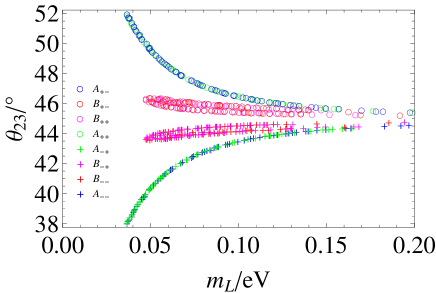
For the normal ordering there are four curves in the shape of a “J” and another four in the shape of an “U”. All require a smallest neutrino mass above zero, the ones in U-shape have a larger minimal value than the ones of J-shape. We name the solutions $A^{\rm N}_{\pm\pm}$ and $B^{\rm N}_{\pm\pm}$. The subscript $\pm\pm$ denotes the signs of $\theta_{23}-\pi/4$ and $\delta$ (lying in our convention between $-\pi$ and $\pi$). Interestingly, solutions of type $A$ have values of the CP phase very close to $\pm\pi/2$, where $-\pi/2$ seems to be preferred by current data Elevant and Schwetz (2015). The type $A$ solutions always keep the signs of $\theta_{23}-\pi/4$ and $\delta$, those of type $B$ only for most of the parameter space. While the lower limit on the smallest mass is 0.034 eV for type $A$, it is 0.046 eV for type $B$.

There are similar types of solutions for the inverted mass ordering, denoted $A^{\rm I}_{\pm\pm}$ and $B^{\rm I}_{\pm\pm}$ (having smallest masses of at least 0.034 and 0.053 eV, respectively). In addition, there is a different type of solution denoted $C^{\rm I}_{\pm}$, where the subscript denotes the sign of $\theta_{23}-\pi/4$. These two cases are special in the sense that they allow only a smallest mass between 0.004 and 0.013 eV. Example solutions are given in Table 2. Note that some of the solutions with $\delta\to-\delta$ are connected by complex conjugation of the mass matrix.

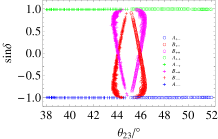
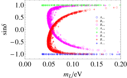
Figure 2: Predicted relations from our model for the normal mass ordering.

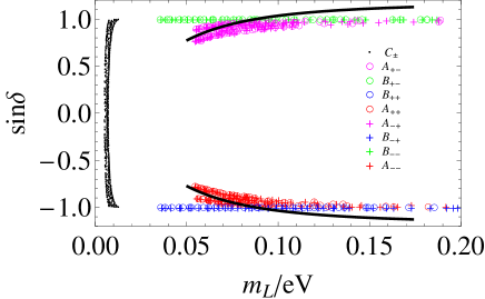
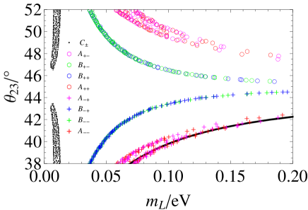
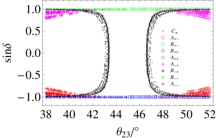
Figure 3: Predicted relations from our model for the inverted mass ordering. The black curves represent analytical results (see Eqs. (31, 32) for explicit expressions) obtained from an approximate calculation, being well compatible with the numerical result.

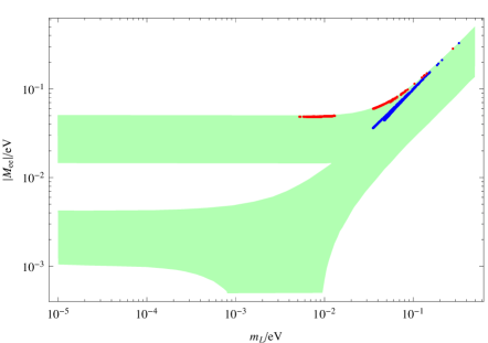
Figure 4: The effective Majorana mass $M_{ee}$ in neutrinoless double beta decay for both normal (blue) and inverted mass ordering (red, note the isolated red points corresponding to the $C^{\rm I}_{\pm}$ solutions). The green shaded area represents the currently allowed parameter space.

The correlation between the interesting parameters $\theta_{23}$, $\delta$ and $m_{L}$ are given in Figs. 2 and 3, respectively. Finally, Fig. 4 summarizes the prediction of the model for neutrinoless double beta decay Rodejohann (2011). We see in particular that for the inverted ordering it always holds that the effective mass takes essentially its largest possible values and that for the normal mass ordering the effective mass is non-zero.

IV.2 Analytical calculation

Now we try to analytically find approximate expressions for one of the many possible solutions. From Table 2 we see that there are solutions with $r_{2}$ and $r_{3}$ close to one. Focusing on this case, we introduce the small parameters

$$\delta_{2}\equiv r_{2}-1\,,\thinspace\delta_{3}\equiv r_{3}-1$$ (27)

in Eq. (26). In this case the neutrino mixing should be close to tri-bimaximal mixing (TBM) because if $\delta_{2},\delta_{3}=0$ the neutrino mixing is TBM. We further assume for simplicity that the neutrino mass sum-rule as discussed at the end of Sec. III holds, which is approximately true in this case as well.

The deviation from TBM can be computed perturbatively under the assumption $\delta_{2},\thinspace\delta_{3}\ll 1$ and some details are found in the Appendix. The result turns out to be

$$U\approx U_{{\rm TBM}}+\left[\begin{array}[]{ccc}(\delta_{2}+\delta_{3})f_{11}(z)&(\delta_{2}+\delta_{3})f_{12}(z)&f_{13}(z)(\delta_{2}-\delta_{3})\\ .&.&f_{23}(z)(\delta_{2}-\delta_{3})\\ .&.&f_{33}(z)(\delta_{2}-\delta_{3})\end{array}\right],$$ (28)

where $z$ first appears in Eq. (24) and the $f$-functions are given in the appendix. The elements not given can be found there, but are not important here.

The important point is that the deviations of $U_{e1}$ and $U_{e2}$ are proportional to $(\delta_{2}+\delta_{3})$ while the deviations of $U_{e3}$, $U_{\mu 3}$ and $U_{\tau 3}$ are proportional to $(\delta_{2}-\delta_{3})$. Note that $U_{e1}$ and $U_{e2}$ determine the value of $\theta_{12}$, which should not be too far away from the TBM value $\sin\theta_{12}=1/\sqrt{3}$. At the same time, $U_{e3}\propto\delta_{2}-\delta_{3}$ should be relatively large compared to the deviation of $\theta_{12}$. Thus, we simplify the analysis further by taking $\delta_{3}=-\delta_{2}$. Another assumption to make our life simpler is that $|1+z|\approx 1$, which implies

$$z\approx e^{2i\alpha}-1\,.$$

The reason for this assumption is as follows: as mentioned above, we use that the actual mass spectrum $(m_{1},m_{2},m_{3})$ is still very close to the leading order one which is proportional to $(\frac{1}{1+z},1,\frac{-1}{1-z})$. With $\delta m^{2}/\Delta m^{2}\ll 1$ it follows $(1-|\frac{1}{1+z}|^{2})/(1-|\frac{1}{1-z}|^{2})\ll 1$ which implies $|1+z|$ should be very close to $1$. Note that if we assume $z\approx e^{2i\alpha}-1$, we are limited to the inverted ordering because $|\frac{1}{1-z}|^{2}$ is always less than $1$.

With the above assumptions (first taking $\delta_{3}=-\delta_{2}$ and then $z\approx e^{2i\alpha}-1$), Eq. (28) can be simplified to

$$U\approx\left(\begin{array}[]{ccc}\sqrt{\frac{2}{3}}&\frac{1}{\sqrt{3}}&g_{13}(\alpha)\delta_{2}\\ .&.&g_{23}(\alpha)\delta_{2}+\frac{1}{\sqrt{2}}\\ .&.&g_{33}(\alpha)\delta_{2}+\frac{1}{\sqrt{2}}\end{array}\right),$$ (29)

where

$$g_{13,23,33}(\alpha)\equiv\frac{3-i\cot\alpha}{3\sqrt{2}},\frac{-3+2i\cot\alpha}{3\sqrt{2}},\frac{3-2i\cot\alpha}{3\sqrt{2}}.$$ (30)

Note that with $|g_{13}(\alpha)|\delta_{2}=\sin\theta_{13}$ we can replace $\delta_{2}$ with $s_{13}/|g_{13}(\alpha)|$ and then extract $\tan\theta_{23}$ and $\sin\delta$ from Eq. (29). They can be expressed in terms of $\theta_{13}$ and $\alpha$,

$$\begin{array}[]{c}\tan\theta_{23}\approx\left|\frac{-2s_{13}z_{2}+i\sqrt{2}|z_{1}|}{2s_{13}z_{2}+i\sqrt{2}|z_{1}|}\right|,\\ \sin\delta\approx\textrm{Im}\left[\frac{z_{1}\left(\sqrt{2}iz_{2}s_{13}+|z_{1}|\right)\left(\sqrt{2}z_{3}s_{13}+2i|z_{1}|\right)}{2|z_{1}|^{3}}\right],\end{array}$$ (31)

where

$$z_{1} \equiv \cot\alpha-3i\,,$$

$$z_{2} \equiv 2\cot\alpha+3i\,,$$

$$z_{3} \equiv 3\cot\alpha+3i\,.$$

Now we have derived approximate expressions for $\theta_{23}$ and $\delta$ in terms of $\alpha$. The value of $\alpha$ can be related to the lightest neutrino mass $m_{L}$ via

$$m_{L}(\alpha)\approx\sqrt{\frac{1}{8}\Delta m^{2}\csc^{2}\alpha}$$ (32)

because the mass spectrum is $(m_{1}^{2},m_{2}^{2},m_{3}^{2})\approx m^{2}(1,1,|1+z|^{-2})$ in our approximation. From Eq. (31) we can extract the following limit

$$\lim_{\alpha\rightarrow 0}\tan\theta_{23}=\lim_{\alpha\rightarrow 0}1-\frac{6\sqrt{2}s_{13}}{8s_{13}^{2}+1}|\tan\alpha|=1\,,$$ (33)

which implies $\alpha$ should be a small angle to make $\theta_{23}$ close to $45^{\circ}$. The limits of Eqs. (31, 32) can also be computed, resulting in

$$\lim_{\alpha\rightarrow 0^{\pm}}\sin\delta=\pm(3\cos 2\theta_{13}-4)\approx\pm 1$$ (34)

and

$$\lim_{\alpha\rightarrow 0}m_{L}(\alpha)\propto\frac{\sqrt{\Delta m^{2}}}{|\alpha|}\,.$$ (35)

Note the limit of $|\sin\delta|$ in Eq. (34) is larger than $1$ since $4-3\cos 2\theta_{13}=1+6\theta_{13}^{2}+\mathcal{O}(\theta_{13}^{3})$. This is due to the inaccuracy of our approximate calculation where we omit all second-order corrections of $\delta_{2}$. The limit (35) implies that small $\alpha$ results in large $m_{L}$, i.e. $m_{L}\rightarrow\infty\Longleftrightarrow\alpha\rightarrow 0$. Therefore, for small $|\theta_{23}-45^{\circ}|$ the smallest mass $m_{L}$ is large. Furthermore, the larger $\alpha$ the larger is the deviation of $\theta_{23}$ from $\pi/4$, which means that there should be a lower bound on $m_{L}$. The above expressions also imply that $\lim_{m_{L}\rightarrow\infty}|\sin\delta|=1$, i.e. as neutrino mass increases the CP phase approaches one of its maximal values.

Those features can be identified from the plots in Fig. 3, showing the accurateness of the analytical study.

IV.3 Phenomenological summary

Let us summarize the phenomenological consequences of the model.

First of all, the lightest neutrino mass cannot be zero or too small, quantitatively summarized from the previous results as follows:

$${\rm normal:}\thinspace m_{L}\mathrel{\hbox to0.0pt{\raise 2.20013pt\hbox{$>$}\hss}{\lower 2.20013pt\hbox{$\sim$}}} 0.034\leavevmode\nobreak\ \textrm{eV,}$$

$${\rm inverted:}\thinspace m_{L}\in (0.004,0.013)\,{\rm or}\,m_{L}\mathrel{\hbox to0.0pt{\raise 2.20013pt\hbox{$>$}\hss}{\lower 2.20013pt\hbox{$\sim$}}}0.034\leavevmode\nobreak\ \textrm{eV.}$$

The lower bound of $m_{L}$ for normal ordering has an important implication as the effective mass $M_{ee}$ is always non-zero. One finds

$${\rm normal:}\thinspace M_{ee}\mathrel{\hbox to0.0pt{\raise 2.20013pt\hbox{$>$}\hss}{\lower 2.20013pt\hbox{$\sim$}}} 0.036\leavevmode\nobreak\ \textrm{eV,}$$

$${\rm inverted:}\thinspace M_{ee}\in (0.0482,0.0493)\,{\rm or}\,M_{ee}\mathrel{\hbox to0.0pt{\raise 2.20013pt\hbox{$>$}\hss}{\lower 2.20013pt\hbox{$\sim$}}}0.059\leavevmode\nobreak\ \textrm{eV.}$$

We also note that for large $m_{L}$ ($\gtrsim 0.1\,\,{\rm eV}$),

$$m_{L}\approx M_{ee}\,.$$ (36)

This is due to the (approximately valid) sum-rule $2m_{2}^{-1}+m_{3}^{-1}=m_{1}^{-1}$ which will give the above relation for a quasi-degenerate spectrum Barry and Rodejohann (2011).

Another important feature of our model is the maximal CP violation. As we can see from the top plots in Figs. 2 and 3, both the $A^{\rm N}$ and $A^{\rm I}$ types of solution (green and blue points) always have maximal $|\sin\delta|$ with very little uncertainties. For the $B^{\rm N}$ and $B^{\rm I}$ types of solution, if $m_{L}$ is large enough, $|\sin\delta|$ also approaches its maximal value. This can be understood e.g. from our previous analytic computation which gives $\lim_{m_{L}\rightarrow\infty}|\sin\delta|=1$.

The $C^{\rm I}$ solution in general do not have maximal CP violation. However, from the lower plot in Fig. 3 we see that $\delta$ and $\theta_{23}$ are strongly correlated (black dots). If $\theta_{23}$ turns out to deviate significantly from $45^{\circ}$ such as $\theta_{23}<42^{\circ}$ or $\theta_{23}>48^{\circ}$, then the $C^{\rm I}$ solutions also predict maximal $|\sin\delta|$.

The two bottom plots in Figs. 2 and 3 show that if large $|\theta_{23}-45^{\circ}|$ is observed in the future, then $|\sin\delta|$ must be close to its maximal value. For the inverted ordering this requires $|\theta_{23}-45^{\circ}|\gtrsim 3^{\circ}$, as just discussed, while for the normal ordering it requires $|\theta_{23}-45^{\circ}|\gtrsim 1.5^{\circ}$. It is interesting to note that such a deviation of $\theta_{23}$ and a maximal $|\sin\delta|$ are simultaneously (still rather mildly) preferred by current global fit as the best-fit of $(\theta_{23},\sin\delta)$ is $(41.4^{\circ},-0.94)$ for normal ordering and $(42.4^{\circ},-0.83)$ for inverted ordering Capozzi et al. (2014).

Finally, since in the large $m_{L}$ limit $\theta_{23}$ goes to $45^{\circ}$, a significant deviation of $\theta_{23}$ from $45^{\circ}$ implies an upper bound on $m_{L}$. For example if $|\theta_{23}-45^{\circ}|\gtrsim 3^{\circ}$ in the normal ordering then from Fig. 2 we get $m_{L}\lesssim 0.06$ eV, which constrains $m_{L}$ to a very narrow region $(0.034,0.06)$ eV.

It is also possible to rule out a mass ordering in this model due to the different structures of solutions. For example, if the future bound on $m_{L}$ is pushed below $0.034$ eV, then only the $C^{\rm I}$ solutions survive. Also, since $(\theta_{23},\delta)$ shown in the bottom plots in Figs. 2, 3 have very different distributions for both possible mass orderings, it is also possible to distinguish them with precise measurements on $\theta_{23}$ and $\delta$.

In summary, if $m_{L}$ is large, we have clear predictions on $\delta$, $\theta_{23}$ and $M_{ee}$, which should be close to their large $m_{L}$ limit

$$\lim_{m_{L}\rightarrow\infty}(|\sin\delta|,\theta_{23},M_{ee})=(1,45^{\circ},m_{L})\,.$$ (37)

If $m_{L}$ is small, then we have some more interesting predictions among these parameters, such as large deviations from $\theta_{23}=45^{\circ}$, correlations between $\theta_{23}$ and $\delta$ as well as with the mass ordering.

V Conclusion

We presented in this model a flavor symmetry model based on $A_{4}$ within a left-right symmetric framework. Various aspect exist that make this environment different from the usual model building. This includes the necessity to treat the particles in left- and right-handed doublets, but more crucially the fact that residual symmetries from breaking the full flavor group do not make it in the mass matrices and hence do not determine the mixing. Furthermore, the discrete left-right symmetry should be parity rather than charge conjugation, in order to avoid inconsistencies between the flavor and charge conjugation symmetries.

Taking all this into account, we were discussing a left-right symmetric model with $A_{4}$ flavor symmetry and analyzed its predictions. No flavor changing neutral currents from the Higgs bi-doublet are present. Several distinct solutions for the neutrino sector were possible, many of which prefering maximal CP violation as currently prefered by data. Various other predictions and correlations exist which would allow for tests of the model.

The various constraints that left-right symmetric theories impose on flavor symmetry models will allow for further analyses, both conceptual as well as phenomenological. The possibility to use left-right symmetry as a first bottom-up step to approach GUT flavor symmetries is another attractive option to study. Such endevours will be left for future studies.

Appendix A Approximate diagonalization of Majorana mass matrices

A.1 General formulae

If a Majorana mass matrix can be written as

$$M=M_{0}+\delta M\,,$$ (38)

where $\delta M\ll M_{0}$ and $M_{0}$ can be diagonalized by $U_{0}$

$$U_{0}^{T}M_{0}U_{0}={\rm diag}(m_{1},m_{2},m_{3})\,,$$ (39)

then $M$ can be approximately diagonalized by $U$

$$U^{T}MU\approx{\rm diag}(m_{1}+\delta m_{1},m_{2}+\delta m_{2},m_{3}+\delta m_{3})\,,$$ (40)

where $U$ can be computed as

$$\begin{array}[]{c}U\approx U_{0}(1+iT)\,,\\ T_{ij}=\frac{i(A_{ij}m_{i}^{*}+A_{ij}^{*}m_{j})}{|m_{i}|^{2}-|m_{j}|^{2}}\thinspace(i\neq j),\thinspace T_{ii}=0\,,\\ A\equiv U_{0}^{T}\delta MU_{0}\,,\,\,\,\delta m_{i}=A_{ii}\,.\end{array}$$ (41)

The above formulae only hold for $T_{ij}\ll 1$, which requires not only $\delta M\ll M_{0}$ but also $|m_{i}|^{2}-|m_{j}|^{2}$ are not very small, i.e. degeneracies in the zeroth-order mass spectrum would invalidate the approximate diagonalization.

These formulae can be derived as follow. Note that

$$U_{0}^{T}MU_{0}=\left(\begin{array}[]{ccc}m_{1}\\ &m_{2}\\ &&m_{3}\end{array}\right)+A$$ (42)

is quasi-diagonal and we need to perform a small rotation $1+iT$ where $T=T^{\dagger}$ and $T\ll 1$ to diagonalize it:

$$\left(\begin{array}[]{ccc}m_{1}\\ &m_{2}\\ &&m_{3}\end{array}\right)+A=(1-iT)^{T}\left(\begin{array}[]{ccc}\tilde{m}_{1}\\ &\tilde{m}_{2}\\ &&\tilde{m}_{3}\end{array}\right)(1-iT).$$ (43)

We can assume $T_{ii}=0$ because if we rephase each column of $U$, i.e. $U\rightarrow U{\rm diag}(e^{i\alpha_{1}},e^{i\alpha_{2}},e^{i\alpha_{3}})$, $U$ still can diagonalize $M$ and any non-zero $T_{ii}$ can be absorbed into such rephasing.

The next-to-leading order in Eq. (43) gives

$$A\approx-i\left(\begin{array}[]{ccc}0&t_{12}&t_{13}\\ .&0&t_{23}\\ .&.&0\end{array}\right)+\left(\begin{array}[]{ccc}\delta m_{1}\\ &\delta m_{2}\\ &&\delta m_{3}\end{array}\right),$$

where

$$t_{ij}\equiv T_{ji}m_{j}+T_{ij}m_{i}\,\leavevmode\nobreak\ ,\delta m_{i}=\tilde{m_{i}}-m_{i}\,.$$

So we have

$$A_{ij}=-i(T_{ji}m_{j}+T_{ij}m_{i})$$

and its conjugate

$$A_{ij}^{*}=i(T_{ij}m_{j}^{*}+T_{ji}m_{i}^{*})\,.$$

Now we can solve the above two equations with respect to $T_{ij}$ and $T_{ji}$ to get Eq. (41).

A.2 Diagonalization of the neutrino mass matrix in the model

We use the general formulae to diagonalize Eq. (26). First we compute $A$ defined in Eq. (41)

$$A=m\left(\begin{array}[]{ccc}\frac{\delta_{2}+\delta_{3}}{3(z+1)}&-\frac{(z+2)\left(\delta_{2}+\delta_{3}\right)}{3\sqrt{2}(z+1)}&\frac{z\left(\delta_{3}-\delta_{2}\right)}{\sqrt{3}\left(z^{2}-1\right)}\\ -\frac{(z+2)\left(\delta_{2}+\delta_{3}\right)}{3\sqrt{2}(z+1)}&\frac{2}{3}\left(\delta_{2}+\delta_{3}\right)&\frac{z\left(\delta_{2}-\delta_{3}\right)}{\sqrt{6}(z-1)}\\ \frac{z\left(\delta_{3}-\delta_{2}\right)}{\sqrt{3}\left(z^{2}-1\right)}&\frac{z\left(\delta_{2}-\delta_{3}\right)}{\sqrt{6}(z-1)}&\frac{\delta_{2}+\delta_{3}}{z-1}\end{array}\right),$$

and then $T$ from Eq. (41)

$$T=\left(\begin{array}[]{ccc}0&\frac{i(3z+(z+1)z^{*}+4)\left(\delta_{2}+\delta_{3}\right)}{3\sqrt{2}\left(|z|^{2}+z+z^{*}\right)}&\frac{i(z(z^{*}-1)+\Re(z))\left(\delta_{2}-\delta_{3}\right)}{2\sqrt{3}\Re(z)}\\ .&0&\frac{(izz^{*}+2\Im(z))\left(\delta_{2}-\delta_{3}\right)}{\sqrt{6}\left(|z|^{2}-2\Re(z)\right)}\\ .&.&0\end{array}\right).$$

So from $U$ in Eq. (41) we get

$$U_{e1}=\frac{\frac{(z+(z+3)z^{*}+4)\left(\delta_{2}+\delta_{3}\right)}{|z|^{2}+z+z^{*}}+6}{3\sqrt{6}}$$

$$U_{e2}=\frac{3-\frac{(3z+(z+1)z^{*}+4)\left(\delta_{2}+\delta_{3}\right)}{|z|^{2}+z+z^{*}}}{3\sqrt{3}}$$

$$U_{e3}=-\frac{z|z|^{2}(z^{*}-1)\left(\delta_{2}-\delta_{3}\right)}{3\sqrt{2}\left(|z|^{2}-2\Re(z)\right)\Re(z)}$$

$$U_{\mu 1}=\frac{\frac{3\left(|z|^{2}+z-\Re(z)\right)\left(\delta_{2}-\delta_{3}\right)}{\Re(z)}+\frac{2(z+(z+3)z^{*}+4)\left(\delta_{2}+\delta_{3}\right)}{|z|^{2}+z+z^{*}}-6}{6\sqrt{6}}$$

$$U_{\mu 2}=\frac{\frac{3(z+(z-1)z^{*})\left(\delta_{2}-\delta_{3}\right)}{|z|^{2}-2\Re(z)}+\frac{(3z+(z+1)z^{*}+4)\left(\delta_{2}+\delta_{3}\right)}{|z|^{2}+z+z^{*}}+6}{6\sqrt{3}}$$

$$U_{\mu 3}=\frac{\frac{(z(z^{*}-1)+\Re(z))\left(\delta_{2}-\delta_{3}\right)}{\Re(z)}-\frac{2\left(|z|^{2}-z+z^{*}\right)\left(\delta_{2}-\delta_{3}\right)}{|z|^{2}-2\Re(z)}+6}{6\sqrt{2}}$$

$$U_{\tau 1}=\frac{\frac{3\left(|z|^{2}+z-\Re(z)\right)\left(\delta_{2}-\delta_{3}\right)}{\Re(z)}-\frac{2(z+(z+3)z^{*}+4)\left(\delta_{2}+\delta_{3}\right)}{|z|^{2}+z+z^{*}}+6}{6\sqrt{6}}$$

$$U_{\tau 2}=\frac{\frac{3(z+(z-1)z^{*})\left(\delta_{2}-\delta_{3}\right)}{|z|^{2}-2\Re(z)}-\frac{(3z+(z+1)z^{*}+4)\left(\delta_{2}+\delta_{3}\right)}{|z|^{2}+z+z^{*}}-6}{6\sqrt{3}}$$

$$U_{\tau 3}=\frac{-\frac{(z(z^{*}-1)+\Re(z))\left(\delta_{2}-\delta_{3}\right)}{\Re(z)}+\frac{2\left(|z|^{2}-z+z^{*}\right)\left(\delta_{2}-\delta_{3}\right)}{|z|^{2}-2\Re(z)}+6}{6\sqrt{2}}$$

The $f$-functions used in Eq. (28) can be extract from above results, for example,

$$f_{11}(z)\equiv\frac{(z+3)z^{*}+z+4}{3\sqrt{6}\left(|z|^{2}+z^{*}+z\right)},$$ (44)

$$f_{12}(z)\equiv-\frac{(z+1)z^{*}+3z+4}{3\sqrt{3}\left(|z|^{2}+z^{*}+z\right)},$$ (45)

$$f_{13}(z)\equiv-\frac{z|z|^{2}(z^{*}-1)}{3\sqrt{2}\Re(z)\left(|z|^{2}-2\Re(z)\right)}.$$ (46)