Online Buy-at-Bulk Network Design
Abstract
We present the first non-trivial online algorithms for the non-uniform, multicommodity buy-at-bulk (MC-BB) network design problem. Our competitive ratios qualitatively match the best known approximation factors for the corresponding offline problems. In particular, we show
-
•
A polynomial time online algorithm with a poly-logarithmic competitive ratio for the MC-BB problem in undirected edge-weighted graphs.
-
•
A quasi-polynomial time online algorithm with a poly-logarithmic competitive ratio for the MC-BB problem in undirected node-weighted graphs.
-
•
For any fixed , a polynomial time online algorithm with a competitive ratio of (where is the number of demands, and hides polylog factors) for MC-BB in directed graphs.
-
•
Algorithms with matching competitive ratios for the prize-collecting variants of all the above problems.
Prior to our work, a logarithmic competitive ratio was known for undirected, edge-weighted graphs only for the special case of uniform costs (Awerbuch and Azar, FOCS 1997), and a polylogarithmic competitive ratio was known for the edge-weighted single-sink problem (Meyerson, SPAA 2004). To the best of our knowledge, no previous online algorithm was known, even for uniform costs, in the node-weighted and directed settings.
Our main engine for the results above is an online reduction theorem of MC-BB problems to their single-sink (SS-BB) counterparts. We use the concept of junction-tree solutions (Chekuri et al., FOCS 2006) that play an important role in solving the offline versions of the problem via a greedy subroutine – an inherently offline procedure. Our main technical contribution is in designing an online algorithm using only the existence of good junction-trees to reduce an MC-BB instance to multiple SS-BB sub-instances. Along the way, we also give the first non-trivial online node-weighted/directed single-sink buy-at-bulk algorithms. In addition to the new results, our generic reduction also yields new proofs of recent results for the online node-weighted Steiner forest and online group Steiner forest problems.
1 Introduction
In a typical network design problem, one has to find a minimum cost (sub) network satisfying various connectivity and routing requirements. These are fundamental problems in combinatorial optimization, operations research, and computer science. To model economies of scale in network design, Salman et al. [32] proposed the buy-at-bulk framework, which has been studied extensively over the last two decades (e.g., [6, 20, 33, 22, 29, 28, 15, 14]). In this framework, each network element is associated with a sub-additive function representing the cost for a given utilization. Given a set of connectivity demands comprising source-sink pairs, the goal is to route integral flows from the sources to the corresponding sinks concurrently to minimize the total cost of the routing.
An important application of the problem is capacity planning in telecommunication networks or in the Internet. As observed by Awerbuch and Azar [6], this application is inherently “online” in that terminal-pairs arrive over time and need to be served without knowledge of future pairs. The authors of [6] give a logarithmic-competitive online algorithm for the uniform case where every edge is associated with the same cost function. However, uniformity is not always a feasible assumption, especially in heterogeneous, dynamic networks like the Internet. Indeed recent research (e.g., [29, 28, 15]) has focused on the non-uniform setting with a different sub-additive function for every network element. In this non-uniform setting, Meyerson [28] gives a polylogarithmic-competitive algorithm for the special case when all terminal-pairs share the same sink. To the best of our knowledge, no non-trivial online algorithm is known for the general multicommodity setting, which is the focus of our paper.
We consider, in increasing order of generality, undirected edge-weighted graphs, undirected node-weighted graphs, and directed edge-weighted graphs.111In undirected graphs, node costs can simulate edge costs; in directed graphs they are equivalent. It is also convenient to classify the problems that we study into the single-sink version where all the terminal-pairs share a common sink, and the general multicommodity version where the sinks in the terminal-pairs may be distinct. For notational convenience, we use the following shorthand forms for our problems: X-Y-BB where X = SS or MC (single-sink and multicommodity, respectively) and Y = E or N or D (undirected edge-weighted, undirected node-weighted, and the general directed case, respectively).
1.1 Our Contributions
We obtain the following new results (unless otherwise noted, our algorithms run in polynomial time):
-
•
A poly-logarithmic competitive online algorithm for the MC-E-BB problem.
-
•
A poly-logarithmic competitive online algorithm for MC-N-BB and SS-N-BB that runs in quasi-polynomial time.
-
•
An -competitive online algorithm for MC-D-BB for any constant with running time , where hides polylogarithmic factors. For SS-D-BB, the ratio improves to , translating to a polylogarithmic competitive ratio in quasi-polynomial time.
-
•
Online algorithms for prize-collecting versions of all the above problems with the same competitive ratio.
Up to exponents in the logarithm, our online algorithms match the best known offline approximation algorithms (Chekuri et al. [15] for MC-E/N-BB and Antonakopoulos [5] for MC-D-BB); for MC-N-BB, however, a polynomial time, polylogarithmic approximation is known [14], whereas our algorithm runs in quasi-polynomial time. Furthermore, a logarithmic lower bound, even for SS-E-BB, follows from the lower bound for the online Steiner tree problem [26], and a polylogarithmic lower bound for online SS-N-BB follows from a matching one for set cover [3].
From a technical perspective, we derive all the multicommodity results using a generic online reduction theorem that reduces a multicommodity instance to several single-sink instances, for which we either use existing online algorithms or give new online algorithms. Informally, one can view this as the “online analog” of the junction-tree approach pioneered by Chekuri et al. [15] for offline multicommodity network design. We discuss this approach in the next subsection.
1.2 An Online Reduction to Single Sink Instances
Multicommodity network design problems, both online and offline, are typically more challenging than their single-sink counterparts, and have historically222For instance, compare [29] and [12] for the SS-E-BB and MC-E-BB problem, and compare Naor et al. [31] and Hajiaghayi et al. [24] for the online node-weighted Steiner tree and Steiner forest problem. required new ideas every time depending on the specific problem at hand. The situation is no different for buy-at-bulk, both for uniform and non-uniform costs.
In the offline buy-at-bulk setting, this shortcoming is addressed by Chekuri et al. [15] (expanded to other problems by [14, 13, 5]), who introduce a generic combinatorial framework for mapping a single instance of a multicommodity problem to multiple instances of the corresponding single-sink problem. At the heart of this scheme is the following observation that holds for many multicommodity problems such as (edge/node) Steiner forest, directed Steiner network, buy-at-bulk, and set connectivity: there exists a near-optimal333We call the quality of such a solution the junction-tree approximation factor; e.g., it is for MC-E-BB and MC-N-BB [15] junction-tree solution for the multicommodity problem that decomposes into solutions to multiple single-sink problems where each single-sink problem connects some subset of the original terminal-pairs to a particular root.
The problem now reduces to finding good junction-trees to cover all the terminal-pairs. The offline techniques [15, 13, 5] tackle this using a greedy algorithm for finding the single-sink solutions; more precisely, in each step they find the best density (cost per terminal-pair) solution that routes a subset of terminal-pairs via a single sink. A set cover style analysis then bounds the loss for repeating this procedure until all terminal-pairs are covered. However, as the reader may have already noticed, the greedy optimization approach is inherently offline, as finding the best-density solution requires knowledge of all terminal-pairs upfront. Our main technical contribution in this work is an online version of the junction-tree framework. Indeed, we show how to reduce any multicommodity buy-at-bulk instance to a collection of single-sink instances online.
(Informal Theorem) If the junction-tree approximation factor of the MC-BB problem is , the integrality gap of a natural LP relaxation of the SS-BB problem is , and there is a -competitive online algorithm for the SS-BB problem, then there is an -competitive algorithm for the MC-BB problem.
To prove the above theorem, we first write a composite-LP, which has (a) an outer-LP comprising assignment variables that fractionally assign terminal-pairs to roots, and (b) many inner-LPs which correspond to the natural LP relaxations for the SS-BB problem for each root and the terminal-pairs fractionally assigned to it by the outer-LP. We then apply the framework of online primal-dual algorithms (see [10] for instance) to solve the composite-LP online. However, there are two main challenges we need to surmount.
First, the existing framework has been mostly applied to purely covering/packing LPs444Our current understanding of mixed packing-covering is limited [7] and does not capture the problem we want to solve. and our inner-LPs have both kinds of constraints, and moreover, there is an outer-LP encapsulating them. We show nonetheless that it can be extended to solving our LP fractionally up to polylogarithmic factors. Indeed, we use the specific flow-structure of the inner-LP, and each step of our algorithm solves many (auxiliary) min-cost max-flow problems.
The second difficulty is in rounding this fractional solution online. This is a hard problem, and currently we do not know how to do so even for basic network design problems such as the Steiner tree problem. To circumvent this, we show that it suffices to only partially round the LP. More precisely, we round the LP solution so that only the outer-LP (assignment variables) become integral, and the inner-LPs remain fractional. This gives us an integral assignment of the terminal-pairs to different single-sink instances, with bounded total fractional cost. Now, from the bounded integrality gap of the inner-LPs, we know that there exist good single-sink solutions for our assignment of terminal-pairs to roots, even though we cannot find them online555The difficulty comes from the fact that the online solution we maintain must be monotonic, i.e., the decisions are irrevocable.. Using this knowledge, our final step is to run online single-sink algorithms for each root, and send the terminal-pairs to the root as determined by the outer-LP assignment. Figure 1 summarizes our overall approach.
initialize multiple online algorithms for the single-sink problem (one for each vertex as root).
when arrives
-
update the fractional solution of the composite LP to satisfy the new request
-
round the composite LP to get an integral solution to the outer LP, which gives us an assignment of to some root
-
send both and to the instance of the single-sink online algorithm with root
The results mentioned in Section 1.1 follow by bounding for the corresponding problems. For MC-E-BB, all of these are known to be ([15, 29, 28] respectively). For MC-N-BB, it is known both are bounded by [14], and we bound in Section 5 by giving the first online algorithms for SS-N-BB. For MC-D-BB, we need some additional work. In this case we cannot directly bound , since the integrality gap of the natural LP relaxation is not known to be bounded. Nevertheless, in Section 4, we show that it suffices to work only with more structured instances for which we can bound the integrality gap.
Finally, we illustrate the generality of our reduction theorem by noting that, when combined with existing bounds on , and , it immediately implies (up to polylogarithmic factors) some recent results in online network design, such as online node-weighted Steiner forest [24], and online edge-weighted group Steiner forest [31] – two problems for which specialized techniques were needed, even though their single-sink counterparts were known earlier.
1.3 Related Work
Buy-at-bulk network design problems have received considerable attention over the last two decades, both in the offline and online settings. For the uniform cost model, Awerbuch and Azar [6] give an -approximation for MC-E-BB, while -approximations are known [20, 33, 22] for SS-E-BB. We also note that -approximations have been obtained in special cases for the multicommodity problem, such as in the rent-or-buy setting [21]. Meyerson et al. [29] give an approximation for the general SS-E-BB, and the first non-trivial algorithm for MC-E-BB is an -approximation due to Charikar and Karagiozova [12]. This was improved to a poly-logarithmic factor by Chekuri et al. [15] who also solve MC-N-BB [14] with similar guarantees. For directed graphs, our knowledge is much sparser. Even for special cases like directed Steiner tree and forest, the best polytime approximation factors known are [34, 11] and [13, 18, 8] respectively, and these ideas were extended to MC-D-BB by Antonakopoulos [5]. On the hardness side, Andrews [4] shows that even the MC-E-BB problem is -hard, while MC-D-BB (in fact directed Steiner forest) is known to be label-cover hard [17].
The online Steiner tree problem (a special case of online SS-E-BB) was first studied by Imase and Waxman [26] who give an -competitive algorithm. Berman and Coulston [9] give an -competitive algorithm for online Steiner forest, and both these results are tight, i.e., there is an lower bound. As mentioned earlier, Awerbuch and Azar’s algorithm [6] can be seen as an -competitive online algorithm for the uniform-cost MC-E-BB. For non-uniform buy-at-bulk, the only online algorithm that we are aware of is Meyerson’s [28] polylog-competitive algorithm for the single-sink problem. For online node-weighted network design, developments are much more recent. A polylogarithmic approximation for the node-weighted Steiner tree problem was first given by Naor et al. [31] and later extended to the online node-weighted Steiner forest problem [24] and prize-collecting versions [23]. These algorithms, like ours in this paper, utilize the online adaptation of the primal-dual and LP rounding schemas pioneered by the work of Alon et al. [3] for the online set cover problem (see also [2] for its adaptation to network design problems). We also note that in the node-weighted setting, the online lower bound can be strengthened to using online set cover lower bounds [3, 27].
2 Preliminaries and Results
We now formally state the problem, set up notation that we use throughout the paper, and state our main theorems.
2.1 Our Problems
Buy-at-bulk Network Design. In the most general setting of the MC-D-BB problem, an instance consists of a directed graph and a collection of terminal-pairs ; each such and is called a terminal. Each pair also has a positive integer demand , which we assume to be for clarity in presentation.666We can handle non-uniform demands by incurring an additional factor in the competitive ratio and the running time (where is the maximum demand) by having “unit-demand” instances, where the instance deals with demands between and . Additionally, each edge is associated with a monotone, sub-additive777That is, whenever , and cost function . A feasible solution to the problem is a collection of paths where is a directed path from to carrying load . Given a solution , we let denote the total load on edge . The goal is to find a feasible solution minimizing the objective . In the online problem, the offline input consists of the graph and the cost functions . The pairs arrive online in an unknown, possibly adversarial, order. When a pair arrives, the algorithm must select the path that connects them, and this decision is irrevocable.
Reduction to the Two-metric Problem. Following previous work, throughout this paper we consider an equivalent problem (up to constant factors) known as two-metric network design. In this problem, instead of functions on the edges, we are given two parameters and on each edge. One can think of as a fixed buying cost, or just cost, of edge , and as a per-unit flow cost, or length, of edge . The feasible solution space is the same as for the buy-at-bulk problem, and the goal is to minimize the objective . The following lemma is well known (see e.g., [15]).
Lemma 1.
Given an instance of the buy-at-bulk problem, for any one can find an instance of the two-metric network design problem such that, for any feasible solution, .
Remark.
In light of the above lemma, henceforth we abuse notation and let the buy-at-bulk problem mean the two-metric network design problem.
2.2 Our Tools
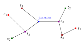
Junction-tree solutions. Given an instance of the buy-at-bulk problem, we consider junction-tree888The word tree is misleading since the final solution need not be a tree in directed graphs. Nevertheless, we continue using this term for historical reasons. Junction trees were originally proposed for undirected graphs, where the solution is indeed a tree. solutions, a specific kind of solution to the problem introduced by [15]. In such solutions, the collection of pairs are partitioned into groups and each group is indexed by a root vertex . For all terminal pairs in a group indexed by , the path from to contains the root vertex (see Figure 2).
Formally, consider an instance of the buy-at-bulk problem, and let denote the objective value of the optimum solution. Given a partition of terminal pairs indexed by different root vertices, a junction-tree solution is one that uses single-sink solutions to connect the original terminal-pairs. Indeed, for each part indexed by root , consider the optimal solutions to the single-sink problem on graph with demands and the single-source problem999The single-source problem in a directed graph is identical to the single-sink problem with all the edges reversed in direction. For undirected graphs, both problems are on the same graph. with pairs . Let denote the sum of the objectives of the optimal solutions to the single-sink and single-source problems, and let . Let denote the minimum over all partitions. We call this solution the optimum junction-tree solution for this instance.101010Note that copies of the same edge appearing in multiple single-sink solutions are treated as distinct edges in the junction-tree solution. Hence, decomposing the optimal multicommodity solution into its constituent paths does not yield . Clearly, . The junction-tree approximation factor of is defined to be the ratio .
LP Relaxation. We now describe a natural flow-based LP relaxation for the single-sink buy-at-bulk problem for an instance where is a set of terminals that need to be connected to the root .
| minimize | (SS-BaB LP) | ||||
| s.t | |||||
2.3 Our Results
Main Technical Theorem and its Applications. Now we are ready to state our main theorem; the proof is in Section 3. We say that an online algorithm is -competitive for a graph if, for any sequence of requests , the online algorithm for buy-at-bulk returns a solution within a -factor of , where .
Theorem 2 (Reduction to Single-Sink Online Algorithms).
Fix an instance of the MC-BB problem. Suppose the following three conditions hold.
-
(i)
The junction-tree approximation factor of is at most .
-
(ii)
The integrality gap of (SS-BaB LP) on any single-sink instance on graph is at most .
-
(iii)
There is a -competitive online SS-BB algorithm for any instance on graph that runs in time .
Then there is an online algorithm for running in time whose competitive ratio is .
Using this theorem, we can immediately obtain the following new results mentioned in the introduction.
Theorem 3 (Undirected Edge-weighted Buy-at-Bulk).
There is a -competitive, polynomial time randomized online algorithm for the MC-E-BB problem.
Proof: The theorem follows directly by combining Theorem 2 with the following results from previous work. Chekuri et al. [15] prove that the junction-tree approximation factor for the undirected edge-weighted buy-at-bulk problem is . Chekuri et al. [16] prove that the integrality gap of (SS-BaB LP) in undirected edge-weighted graphs is . Meyerson [28] gives a randomized polynomial time online algorithm for the single-sink buy-at-bulk problem with competitive ratio .
Theorem 4 (Undirected Node-weighted Buy-at-Bulk).
For any constant , there is an -competitive, randomized online algorithm for MC-N-BB with running time . As a corollary, this yields a -competitive, quasi-polynomial time algorithm for this problem.
Theorem 5 (Directed Buy-at-Bulk).
For any constant , there is an -competitive, polynomial time online algorithm for the MC-D-BB.
We again use Theorem 2 to prove the above theorems. However, unlike for MC-E-BB, we are not aware of any online algorithms for the SS-N-BB and SS-D-BB problems. We therefore first give online algorithms for these problems, and then use Theorem 2; the details appear in Sections 5 and 4.
Finally, we can almost directly use Theorem 2 to also obtain matching results for prize-collecting versions of the above problems. Recall that in a prize-collecting problem, every terminal-pair also comes with a penalty , and the algorithm can opt to not satisfy the request by incurring this value in the objective. We give the extension of our results to the corresponding prize-collecting problems in Section 6.
Theorem 6.
For each of the above problems, there is an online algorithm with matching running time and competitive ratio for the corresponding prize-collecting version.
In addition to the new results mentioned above, we can also use Theorem 2 to give alternative proofs (with slightly worse polylog factors) of some recent results in online network design. By combining Theorem 2 with the -competitive algorithm for online group Steiner Tree due to Alon et al. [2], we obtain a -competitive online algorithm for the group Steiner forest problem – a result shown earlier by Naor et al. [31]. Similarly, by combining Theorem 2 with the -competitive online algorithm for the node-weighted Steiner tree problem due to Naor et al. [31], we obtain a -competitive online algorithm for the node-weighted Steiner forest problem – a result shown earlier by Hajiaghayi et al. [24].
Height Reduction Theorem. One of the technical tools that we use repeatedly in this paper is the following result, which builds on the work of Helvig et al. [25]. We give the proof in Appendix A.
Theorem 7.
Given a directed graph with edge costs and lengths , for all , we can efficiently find an upward directed, layered graph on levels and edges (with new costs and lengths) only between successive levels going from bottom (level ) to top (level ), such that each layer has vertices corresponding to the vertices of , and, for any set of terminals and any root vertex ,
-
(i)
the optimal objective value of the single-sink buy-at-bulk problem to connect (at level ) with (at level ) on the graph is at most , where is the objective value of an optimal solution of the same instance on the original graph ;
-
(ii)
given a integral (resp. fractional solution) of objective value for the single-sink buy-at-bulk problem to connect with on the graph , we can efficiently recover an integral (resp. fractional solution) of objective value at most for the problem on the original graph .
Likewise, we can obtain a downward directed, layered graph on -levels with edges going from top to bottom, with the same properties as above except for single-source instances instead.
3 Proof of Theorem 2 (Online Reduction to Single-Sink Instances)
There are three main steps in the proof. In Section 3.1, we describe the composite LP which is a relaxation of optimal junction-tree solutions (for technical reasons, we first need to pre-process the graph). Next, in Section 3.2, we show how to fractionally solve the LP online. Third, in Section 3.3, we show how to partially round the LP online. The resulting solution then decomposes as fractional solutions to different single-sink instances. Finally, we use the bounded integrality gap and the online algorithm for SS-BB to wrap up the proof in Section 3.4.
3.1 The Composite-LP Relaxation: MC-BaB LP
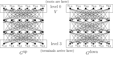
We first apply Theorem 7 with to obtain layered graphs (resp., ) of height where all the edges are directed upward (resp. downward); see Figure 3 for an illustration. The reason for this preprocessing is that the length of the paths appear as a factor in our final competitive ratio and the above step bounds it to a logarithmic factor. Recall that the graph (resp., ) approximately preserves the single-sink (resp., single-source) solutions for any set of terminals and any root. After this step, we can imagine that all the roots (of the single-sink instances we will solve) are vertices in level , and all the terminals will be vertices in level . For clarity of presentation, we refer to the root and terminal vertices by the same name in both and (even though the graphs are completely disjoint). Overloading notation, let denote the vertices in level in both and , and let be the union of the edge sets of and . Furthermore, the cost and length of these edges are inherited from Theorem 7.
Now, using the junction-tree decomposition with approximation factor , we get the following lemma.
Lemma 8.
There exists a set of root vertices, a partition of the terminal-pairs in , a collection of in-trees rooted at in , and a collection of out-trees rooted at in such that
-
(i)
Each belongs to for some .
-
(ii)
For each , the in-tree is a feasible solution to the single-sink buy-at-bulk problem connecting to in ; likewise, the out-tree is a feasible solution to the single-source buy-at-bulk problem connecting to in .
-
(iii)
The sum of objective values of the single-source and single-sink solutions is at most .
Proof: Since the junction-tree approximation ratio of the given instance is , there exists a junction-tree solution given by a set of roots and a partition such that the total objective value of all the single-sink and single-source junction-trees is at most . Moreover, by Theorem 7, because we choose the height , the objective value of each single-sink and single-source solution in increases by a factor of in and respectively. Thus, the overall objective value of the resulting junction-trees in the graphs and is .
The above lemma motivates the LP relaxation given in Fig. 4 which seeks to assign each pair to some rooted instance, and then minimizes the total fractional objective value of the rooted instances. Each individual rooted instance is represented by an inner-LP (see the boxed constraints in Fig. 4).
| minimize | (MC-BaB LP) | |||||
| s.t | (2a) | |||||
| (2b) | ||||||
| (2c) | ||||||
| (2d) | ||||||
| (2e) | ||||||
| (2f) | ||||||
| (2g) | ||||||
In the LP, denotes the extent to which the pair chooses root to route its flow. Within each inner-LP corresponding to a root , are the variables which denotes whether edge is used to route flow in the corresponding rooted instance, and (resp. ) denotes the amount of flow sends (resp., receives) along to (resp., from) root . Observe that if the variables are integral, then the inner-LP corresponding to every root constitutes a feasible fractional solution to (SS-BaB LP) for the single-sink instance where and the single-source instance where . The next lemma, which bounds the optimal value of the MC-BaB LP, follows directly from Lemma 8.
Lemma 9.
The optimum value of (MC-BaB LP) is .
3.2 An online fractional algorithm for the MC-BaB LP
Theorem 10.
There is a randomized, polynomial-time online algorithm that returns a feasible fractional solution for (MC-BaB LP) of value at most .
In the remainder of the subsection, we prove the above theorem. We remark that the overall reduction uses Theorem 10 as a black-box and the time-constrained reader can skip the proof and move to Section 3.3.
To simplify the exposition, we assume that we know the cost of an optimal solution up to a constant factor, using a standard doubling trick111111Suppose our online algorithm has a competitive ratio of , and the true cost of an optimal solution is . Then, we begin with an initial guess for the optimal cost, and run the online algorithm assuming this guess is the correct estimate for . If our online algorithm fails to find a feasible solution of cost at most times the current guess, we double our guess and run the online algorithm again. Eventually, our guess will exceed the optimal cost by at most a factor of two, and for this guess, the algorithm will compute a feasible solution of cost at most . Moreover, since our guesses double every time, the total cost of the edges bought by the online algorithm over all the runs across different guesses is at most .. Once we know , by re-scaling all the parameters in the problem, we may assume that it equals . Next, we delete any edge in or that has cost or length larger than as such edges cannot participate in any optimal solution. Subsequently, we initialize all variables to . Likewise, we initialize all variables to and also send an initial flow of from each to in on an arbitrary flow path from to and likewise from to in . This setting ensures that the cost of the initial solution is .
In the following, we partition the edge set into disjoint sets , where denotes the set of edges in between levels and . Furthermore, for clarity of exposition, we describe a ‘continuous-time’ version of the algorithm where we increase the variables as a function of time. We note that this algorithm can easily be discretized for a polynomial-time121212The polynomial is in the size of the input to this algorithm, which for some of our algorithms/results is quasi-polynomial in the size of the actual problem instance as stated in the introduction. implementation. The algorithm is given as Algorithm 1.
When a terminal-pair arrives, we update the LP solution using the following steps:
-
(1)
Let denote the set of roots in level such that is connected to in and is connected to in . For each , initialize a flow of value using any arbitrary flow path from to in and likewise from to in . Also set for these roots.
-
(2)
Repeat the following while :
-
(a)
Call an edge tight for root if or .
-
(b)
Edge Update: For all tight edges , update at the rate .
-
(c)
Flow Update: Solve the following min-cost max-flow problem for each : maximize such that
-
-
there exists a flow sending units of flow from to in ,
-
-
there exists a flow sending units of flow from to in ,
-
-
Capacity constraints: and for all tight edges ,
-
-
Cost constraint: and .
-
-
-
(d)
Update at the rate , and at the rate for all , and update at the rate .
-
(a)
We increase the variables on tight edges at a rate inversely proportional to their cost, similar to the well-known online set cover algorithm [3]. However, the “flow constraints” are not pure packing (or covering) constraints and there is no general-purpose way of handling them. Indeed, we determine the rate of increase of the flow variables by solving an auxiliary min-cost max-flow subroutine which routes incremental flows of equal value from to in and from to in respecting capacity constraints (i.e., for edges that are tight, the incremental flow is at most the rate of increase of ). This maintains feasibility in the inner LP. Moreover, to bound the rate of increase in objective, we enforce that the total length of the incremental flow is at most (this is the “cost” constraint in the min-cost max-flow problem). We stress that the incremental flows from the auxiliary problem dictate the rate at which we increase the original flow variables in the LP. The final solution is feasible since the algorithm runs until the outer-LP constraint is satisfied.
First, note that the total cost of initialization is over all the edge and flow variables. So it suffices to bound the cost of the updates. The next lemma relates the total cost of the updates to the total time for which the algorithm runs, and the subsequent lemma bounds in terms of .
Lemma 11.
The LP objective value at the end of the above algorithm is , where is the (continuous) time for which the algorithm runs.
Proof: We show that at any time , the rate of the increase of the LP objective value in the algorithm is at most ; this proves the lemma.131313We remark that the “” corresponds to the number of levels in justifying the preprocessing step before the LP description. The objective increases because of increase in variables and flow variables ; we bound these separately.
We first upper bound the objective increase due to the changes in the variables. Fix a level and let denote the set of tight edges in at time . By definition, (resp., ) equals the total flow on these edges for the pair . Since the edges in form a cut separating from , the total flow across this cut is at most . Since , we have . Now, the rate of increase of each such tight edge is precisely , which implies that the total rate of increase of the LP value due to the increase of is at most
Summing over all levels gives the desired bound.
Next, we upper bound the objective increase due to the changes in the variables. When these variables are updated, the total rate of increase of the objective due to the lengths of the and flow paths is at most — this is precisely the “cost” constraint in the auxiliary flow problem. Hence the total rate of increase of flow lengths is at most , completing the proof.
Given the above lemma, we are left to relate to in order to complete the proof of Theorem 10.
Lemma 12.
The time duration of the above algorithm satisfies .
We will need several new definitions and auxiliary lemmas in order to prove Lemma 12. Recall from Lemma 8 that we can assume that the solution that we are comparing against is the set of junction-trees defined by and for . Also, recall that the terminal-pairs are partitioned by the groups . For every , let denote the path from to the root in such that . Similarly, let denote the path from to in . Let for any path . Lemma 8 asserts that
| (3) |
To bound against the optimal junction-tree solution, we use two sets of charging clocks:
-
•
We maintain an edge clock on every pair such that or , i.e., if is used by the optimal junction-tree solution in the single-source (or single-sink) instance corresponding to . In particular, note that if an edge is in multiple junction-trees, then it has a separate clock for each such tree.
-
•
We maintain a terminal clock on every terminal-pair .
The crucial invariant that we maintain is the following: at any time instant , at least one clock “ticks,” i.e., augments its counter at unit rate. The overall goal would then be to bound the total time for which all the charging clocks can cumulatively tick.
First, we describe the rule for the ticking of the clocks. Fix a time , and let the terminal-pair be the pair that is active at time . Let denote the root vertex which has been assigned to in the optimal junction-tree solution from Lemma 8, i.e., . Now, consider the flow-paths in and in . We can have one of two situations:
-
-
If any variable is tight for any edge at time , then the edge clock on the pair ticks at time . If there are multiple such edges, then all the corresponding clocks tick.
-
-
Otherwise, both paths are free of tight edges. In this case, the terminal clock for ticks at time .
Lemma 13.
For any pair such that , its edge clock ticks for time.
Proof: Notice that is initialized to for all roots , and increases at the rate
| (4) |
at all times when the edge clock on ticks. To see why, consider a time when the clock on ticks, and let denote the active terminal-pair at time . It must be that (i) has been assigned to root in , and (ii) either or . But in this case, we increase such variables at rate in our algorithm (Step (2a)). Therefore, we can infer that the value of would be after the edge clock on has ticked for time . But clearly, cannot be a tight edge for any subsequent terminal-pair once reaches 1; therefore, the edge clock on ticks for time overall.
Lemma 14.
For every terminal-pair connected by the optimal junction-tree solution through the root vertex , the total time for which the terminal clock ticks is at most .
Proof: Recall that if the terminal clock for is ticking at time , then it must mean that no edge is tight on either path or . In this case, we show that the variable increases at a fast enough rate, where is the root is assigned to in the optimal junction-tree, i.e., . We show this by exhibiting a feasible solution to the auxiliary LP considered in Step (2b) of the algorithm for root . Indeed, send the flow from to along , and likewise from to along . Also set the value of to be . Clearly, on the edges of these flow paths, we do not have any capacity constraints since no edge is tight. So, the only constraints are the cost constraints which are satisfied by the choice of . Hence, the rate of increase of is at least
| (5) |
at all times when the terminal clock on ticks. This proves the claim, for otherwise the variable would have reached , and the algorithm would have completed processing .
3.3 Partial Online LP Rounding
We partially round the fractional solution returned by Theorem 10 to obtain integral values for only the outer-LP variables , i.e., each pair is integrally assigned to a root. The inner-LP variables and continue to be fractional but represent unit fractional flow from to and to for the pairs assigned to . The partial rounding algorithm is given as Algorithm 2.
-
(1)
Initialization: Each root chooses a threshold uniformly at random.
-
(2)
Partial Rounding: At each time, maintain the scaled solution , . Also set if .
Theorem 15.
The scaled solution component-wise dominates a feasible solution to the outer-LP, and the expected objective value of the scaled solution is at most . Moreover, for each , there exists at least one root such that with probability at least .
Proof: Since each root chooses its threshold independently and uniformly at random from , the probability that is at least (since if and only if ). Since this is independent for different roots, a standard Chernoff-Hoeffding bound application (see, e.g., [30]) shows that each pair has for some root with probability at least . Moreover, the expected value of any variable is given by
A similar argument shows that the expected values of scaled flow variables are also bounded by times their values in the fractional solution. This shows that the expected objective value of the solution is at most times the value of ; by Theorem 10, the latter is at most . Combining these facts gives us the desired bound on the value of the scaled solution.
It remains to show that the scaled solution dominates a feasible solution to the LP. To this end, fix some root and let denote the set of pairs for which . We need to show that installing capacities of on the edges can support unit flow from to in for all . Suppose for contradiction that there is is a cut separating from of capacity strictly smaller than . This implies that every edge must have ; otherwise, we would have an edge with , which contradicts our assumption on the cut capacity. But then the value of the min-cut is precisely , which must be at least because of the following two observations: (i) we know that is a feasible flow from to of value and hence it must be that , and (ii) since , it must be that . This contradicts the assumption that the cut capacity is strictly smaller than . A similar argument shows that the variables can support unit flow from to for every with .
3.4 Wrapping up: Invoking the Single-Sink Online Algorithm
We are now ready to put all the pieces together and present our overall online multicommodity buy-at-bulk algorithm as Algorithm 3. is the online algorithm for SS-BB alluded to in point (iii) of the statement of Theorem 2.
when arrives
- (1)
- (2)
-
(3)
if: send both and to the instance of with root .
-
(4)
else: buy a trivial shortest path between and on the metric and route along this path
Clearly the algorithm produces a feasible solution; so we now argue about the expected objective value. Fix an pair. Since the probability that a terminal-pair is not assigned to a root is (by Theorem 15), the expected total contribution of such unassigned terminal-pairs is . For a root , let be the terminal-pairs assigned to . We know that restricted to dominates a feasible solution in (SS-BaB LP). Letting denote the contribution of this restriction to the overall LP value, we get . By the integrality gap condition, we get that , i.e. the integral optimum objective value of the instance generated by and , is at most . (Here we are using the fact from Theorem 7 that moving to the layered instance does not increase the integrality gap.) The objective value of the solution produced by is at most , where is the competitive ratio of . Putting these observations together, we conclude that the overall objective value of the solution returned by the online algorithm is . This completes the proof of Theorem 2.
4 Online Directed Buy-at-Bulk
In this section, we prove Theorem 5. A natural approach is to use the reduction given by Theorem 2. To this end, we need to establish the following: the existence of a junction-tree scheme with a good approximation; a good upper bound on the integrality gap for single-sink instances of the LP given in Section 2; and an online algorithm for single-sink instances with a good competitive ratio.
Extending the work of Chekuri et al. [13], Antonakopoulos [5] shows the existence of a junction-tree scheme with approximation . Unfortunately, the integrality gap of the LP relaxation is not very well understood even for Steiner tree instances; [35] gives an lower bound141414However, in these instances, is exponentially large in . So, they do not rule out a upper bound. on the integrality gap for the Steiner tree problem and no suitable upper bound is known. We overcome this difficulty as follows. Instead of working with general graphs, we pre-process the instance and obtain a tree-like graph for which we can show that the LP has a good integrality gap. Finally, we give the first non-trivial online algorithm for the directed single-sink buy-at-bulk problem. These results, together with our reduction (Theorem 2), imply the online algorithm for MC-D-BB.
We devote the rest of this section to the proof of Theorem 5; to aid the reader, we restate the theorem below.
Theorem 16.
For any constant , there is a -competitive, polynomial time randomized online algorithm for the general buy-at-bulk problem.
Pre-processing step. We first give our reduction from general instances of the directed buy-at-bulk problem to much more structured instances; the reduction loses a factor of in the approximation ratio.
Let . Given an instance of the directed buy-at-bulk problem, we map it to a tree-like instance as follows. We start by applying Theorem 7 to to obtain the graphs and ; recall that these graphs are layered -level graphs with vertices (corresponding to the vertices in ) in each level, and the levels are numbered with being called the root level. The graph has edges directed from higher numbered levels to lower numbered levels, and has edges in the opposite direction. To facilitate the construction of the graph , we now create trees from and trees from as follows.
For every “root vertex” at level in (resp. ), the tree (resp. ) is constructed as follows:
-
•
The layer of has just one vertex – the root .
-
•
For each such that , the -th layer of contains all -length tuples where is a vertex present in the -th layer of .
-
•
For every edge , there is an arc from to inheriting the same cost and length .
Therefore each tree is an in-arborescence, with all edges directed towards the root. The tree is constructed analogously except all edges are directed away from the root. In the following, we use the term leaves to refer to the vertices on layer of these trees.
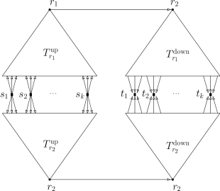
After performing the above operation for every root vertex in level of and , we have trees. Then the final graph is obtained as follows (see Figure 5). For each root , we first add an arc from the root of to of zero cost and length. Finally, for every pair, we add the vertices and to and the following arcs connecting them to the trees: for each tree , we add an arc from to each leaf of of the form with ; for each tree , we add an arc to from each leaf of of the form with . These new arcs have zero cost and length (i.e., ).
This completes the construction of . Note that the graph has vertices and a similar number of edges. Our new instance is and we will apply Theorem 2 to this instance.
We first relate the objective values of and .
Lemma 17.
Every feasible solution for is a junction-tree solution.
Proof: Note that any path in has the following structure: connects to a leaf node of for some , then continues to the root , then traverse the edge to the root of , then goes down to a leaf of and finally connects to . Thus, for any feasible solution for , the pairs can be partitioned based on the root through which they connect.
Lemma 18.
Any feasible solution for can be mapped to a feasible solution — in fact, a junction-tree solution — for of equal or smaller objective value.
Proof: Note that from the previous lemma, any feasible solution in is a junction-tree solution. Therefore, there is a partition of the pairs depending on which root vertex they are using to connect. Moreover, it follows from our construction of the trees in that any edge in (resp. ) corresponds to an edge in (resp. ). Therefore, if we map each edge appearing in solution to its corresponding edge in or , we obtain a mapping from each junction tree of rooted at to a junction tree in rooted at that is connecting the same subset of pairs. Finally, by Theorem 7, each junction tree in rooted at can be mapped, without increasing the objective value, to a junction tree in rooted at that is connecting the same subset of pairs. This completes the proof of the lemma.
Lemma 19.
, where is the objective value of an optimal junction-tree solution for .
Proof: Consider the optimal junction tree solution for . Let the optimum partition be where is the set of roots of the junction trees. For each , let be the set of sources of and be the corresponding sinks. From Theorem 7, we know that the optimum objective value of any one single-sink problem connecting to in is at most times the objective value of the optimum solution connecting each source in to . An analogous upper bound holds for every optimal single-source solution connecting to each sink in . Therefore, we get that the total sum of objective values of each of the junction trees in and is at most . Now notice that any solution for can easily be “simulated” by a solution in the tree : indeed, for every root-vertex path in the solution , include the edge from to in (recall the vertices in exactly correspond to such root-vertex paths). It is easy to see that the objective value of the solution in is the same as that of . Similarly, any solution for can be simulated in with the same objective value. It follows that there is a feasible solution in of objective value at most .
Corollary 20.
.
Proof Sketch: Antonakopoulos [5] shows that there exists a junction-tree solution of cost at most . The corollary follows from this work and the fact that we set .
Now we are ready to show that the new instance has the properties required by the reduction, i.e., Theorem 2 can be applied. In the following lemma, a single-source (resp. single-sink) sub-instance of is a single-source (resp. single-sink) instance of the following form: the graph is the same as in , namely ; the set of terminals is a subset of the sources (resp. sinks) of ; the terminals need to be connected to a root vertex .
Lemma 21.
Let be the instance described above. Let be as in the statement of Theorem 2. We have
-
(i)
The junction-tree approximation factor of is (i.e., ).
-
(ii)
The integrality gap of (SS-BaB LP) for any single-sink/source sub-instance is (i.e., ).
-
(iii)
There is a -competitive algorithm for any single-sink/source sub-instance (i.e., ).
Proof: Property (i) follows from Lemma 17. Thus we focus on proving (ii) and (iii). In the following, we assume that we are working with a single-sink sub-instance of ; the proof is very similar for single-source sub-instances and we omit it.
In order to show (ii) and (iii), we will map the sub-instance to an instance of the group Steiner tree problem on a tree as follows. Since , we have for some . We first consider the case when . In order to define the tree of the group Steiner tree instance, we start with the subtree of rooted at . We add the following ‘dangling’ edges to for each source : for each leaf vertex such that has an edge in to , we add a new vertex to and connect it to . Let be the resulting tree. We assign weights to the edges of as follows. Each of the old edges receives a weight equal to . Each of the new edges receives a weight equal to , where is the path of from to . Finally, we define the following groups: for each source , we introduce a group consisting of all the new vertices such that is connected to its partner in (that is, has an edge from to ). In the resulting group Steiner tree instance, the goal is to connect all of the groups to the root using a minimum weight subtree of ; we let denote this instance.
Now the key claim is that the feasible solutions to the single-sink buy-at-bulk are in a one-to-one correspondence with feasible solution to the group Steiner tree instance ; moreover, the objective value of a solution to the former is equal to the weight of the solution to the latter. To see this, consider a feasible solution for the single-sink buy-at-bulk instance. Note that, for each source , has a path connecting to ; it follows from our construction of that this path consists of an edge from to a leaf of followed by the unique path in from to . Thus we can construct a feasible group Steiner tree solution by connecting each group using the path of from to , where is the partner of the leaf of through which connects to the root in the buy-at-bulk solution. The weight of the edge captures the -cost of ’s path and the weight of the path from to captures the -cost of ’s path.
Moreover, we can apply the same argument to fractional solutions to the two problems and show that there is a bijection between feasible fractional solutions to (SS-BaB LP) and feasible fractional solutions to the LP relaxation for group Steiner tree of Garg, Konjevod, and Ravi [19]; as before, these corresponding solutions have the same objective values. Now the desired upper bound on the integrality gap of (SS-BaB LP) follows from the work of [19] who showed that the integrality gap of the group Steiner tree LP is where is the maximum size of a group and is the number of groups. In our setting, and . Therefore the integrality gap is , which establishes property (ii).
Moreover, notice that the above reduction can also be used to obtain an online algorithm for the single-sink (and single-source) sub-instances. Indeed, we simply use the online group Steiner tree algorithm of Alon et al. [1] which has a competitive ratio . This proves property (iii).
Now we are ready to complete the proof of Theorem 16.
Proof of Theorem 16: Given the instance , we construct the graph as described above; the time taken to do so is . We pass the instance to Theorem 2 and, using Lemma 21, we obtain an online algorithm that, for any collection of pairs and any adversarial ordering of , returns a solution of cost . By Lemma 19 and Corollary 20, we can map solutions for to solutions for .
We note that the approach described above also gives us new online algorithms for the single-sink buy-at-bulk problem on directed graphs. For single-sink instances, the junction-tree approximation is equal to and thus we save a factor of .
Corollary 22.
There is a polynomial time -competitive online algorithm for the single-sink (or single-source) buy-at-bulk problem on directed graphs. The competitive ratio can be improved to if the running time can be quasi-polynomial in .
5 Online Single-sink, Undirected, Node-weighted Buy-at-Bulk
In this section, we prove Theorem 4. Again, we use our main theorem (Theorem 2) and reduce the multi-commodity buy-at-bulk problem to the single-sink version of the problem. We combine the reduction theorem with the following results from previous work. Chekuri et al. [13] show the existence of a junction-tree scheme with approximation factor . Moreover, the natural LP relaxation for the single-sink buy-at-bulk problem on graphs with node costs is also [15]. For the single-source online algorithm, we resort to the algorithms from the previous section for the more general directed single-sink buy-at-bulk problem (see Corollary 22). We now obtain the desired result by the following parameter settings:
6 Online Prize-Collecting Buy-at-Bulk
In the prize-collecting version of the buy-at-bulk problem, each terminal pair also comes with a penalty and the algorithm may choose not to serve this request and incur the penalty in the total cost. We show that our online reduction framework (Theorem 2) can be easily modified to handle prize-collecting versions as follows.
Theorem 23.
Let be a buy-at-bulk instance and suppose the three conditions of Theorem 2 hold. Then there is an -competitive online algorithm for the online, prize-collecting buy-at-bulk problem on with arbitrary penalties.
Proof: We closely follow the proof of Theorem 2. The first difference is in the LP-formulation. Now, for each pair we have an extra variable which indicates whether we choose to discard this pair (and pay the corresponding penalty) or not. We point out the differences with (MC-BaB LP). The new objective function is
and (2a) is replaced by
Observe that the optimum value of this modified LP is at most times the optimum: set for the pairs the integral optimum solution does not connect, and for the rest apply Lemma 9. Also observe that the modified LP can be thought of the old LP on a modified instance where the graphs and (obtained from Theorem 7) have another vertex at the root level, and each has a direct path from to in with total length and no fixed cost, and similarly, each has a path from to in with total length and no fixed cost. The rest of the proof now follows exactly as in Section 3, by also including the special vertex as a possible root while rounding to make the outer LP variables integral.
7 Conclusion
In this paper, we gave the first polylogarithmic-competitive online algorithms for the non-uniform multicommodity buy-at-bulk problem. Our result is a corollary of a generic online reduction technique that we proposed in this paper for converting a multicommodity instance into several single-sink instances, which are often easier to design algorithms for. We believe that this reduction will have other applications beyond the buy-at-bulk framework, and illustrate this by showing that recent results on online node-weighted Steiner forest and online generalized connectivity directly follow from our reduction theorem. Our work also opens up new directions for future research. For instance, our algorithm for the node-weighted problem runs in quasi-polynomial time, and a concrete open question is to get a polynomial-time polylogarithmic-competitive algorithm for the SS-N-BB problem (this suffices for MC-N-BB as well by our main theorem). Another technical question concerns non-uniform demands. While our algorithm can be extended to the case of non-uniform demands, the approximation ratio incurs an additional factor, where is the ratio of the largest to the smallest demand. It would be interesting to eliminate this dependence on since the corresponding offline results do not have this dependence. More generally, a broader question is to investigate other mixed packing-covering LPs that can be solved and rounded online.
Acknowledgements
D. Panigrahi is supported in part by NSF Award CCF-1527084, a Google Faculty Research Award, and a Yahoo FREP Award.
References
- [1] N. Alon, B. Awerbuch, Y. Azar, N. Buchbinder, and J. Naor. A general approach to online network optimization problems. In Proceedings, ACM-SIAM Symposium on Discrete Algorithms (SODA), pages 577–586, 2004.
- [2] N. Alon, B. Awerbuch, Y. Azar, N. Buchbinder, and J. Naor. A general approach to online network optimization problems. ACM Trans. on Alg., 2(4):640–660, 2006.
- [3] N. Alon, B. Awerbuch, Y. Azar, N. Buchbinder, and J. Naor. The online set cover problem. SIAM J. Comput., 39(2):361–370, 2009.
- [4] M. Andrews. Hardness of buy-at-bulk network design. In Proceedings, IEEE Symposium on Foundations of Computer Science (FOCS), pages 115–124, 2004.
- [5] S. Antonakopoulos. Approximating directed buy-at-bulk network design. In Proceedings, Workshop on Approximation and Online Algorithms (WAOA), pages 13–24, 2010.
- [6] B. Awerbuch and Y. Azar. Buy-at-bulk network design. In Proceedings, IEEE Symposium on Foundations of Computer Science (FOCS), pages 542–547, 1997.
- [7] Y. Azar, U. Bhaskar, L. Fleischer, and D. Panigrahi. Online mixed packing and covering. In Proceedings, ACM-SIAM Symposium on Discrete Algorithms (SODA), pages 85–100, 2013.
- [8] P. Berman, A. Bhattacharyya, K. Makarychev, S. Raskhodnikova, and G. Yaroslavtsev. Approximation algorithms for spanner problems and directed steiner forest. Inform. and Comput., 222:93–107, 2013.
- [9] P. Berman and C. Coulston. On-line algorithms for steiner tree problems (extended abstract). In Proceedings, ACM Symp. on Theory of Computing (STOC), pages 344–353, 1997.
- [10] N. Buchbinder and J. Naor. Online primal-dual algorithms for covering and packing. Math. Oper. Res., 34(2):270–286, 2009.
- [11] M. Charikar, C. Chekuri, T. Cheung, Z. Dai, A. Goel, S. Guha, and M. Li. Approximation algorithms for directed steiner problems. J. Algorithms, 33(1):73–91, 1999.
- [12] M. Charikar and A. Karagiozova. On non-uniform multicommodity buy-at-bulk network design. In Proceedings, ACM Symp. on Theory of Computing (STOC), pages 176–182, 2005.
- [13] C. Chekuri, G. Even, A. Gupta, and D. Segev. Set connectivity problems in undirected graphs and the directed steiner network problem. ACM Transactions on Algorithms, 7(2):18, 2011.
- [14] C. Chekuri, M. T. Hajiaghayi, G. Kortsarz, and M. R. Salavatipour. Approximation algorithms for node-weighted buy-at-bulk network design. In Proceedings, ACM-SIAM Symposium on Discrete Algorithms (SODA), pages 1265–1274, 2007.
- [15] C. Chekuri, M. T. Hajiaghayi, G. Kortsarz, and M. R. Salavatipour. Approximation algorithms for nonuniform buy-at-bulk network design. SIAM J. Comput., 39(5):1772–1798, 2010.
- [16] C. Chekuri, S. Khanna, and J. Naor. A deterministic algorithm for the cost-distance problem. In Proceedings, ACM-SIAM Symposium on Discrete Algorithms (SODA), volume 7, pages 232–233, 2001.
- [17] Y. Dodis and S. Khanna. Design networks with bounded pairwise distance. Proceedings, ACM Symp. on Theory of Computing (STOC), pages 750 – 759, 1999.
- [18] M. Feldman, G. Kortsarz, and Z. Nutov. Improved approximation algorithms for directed steiner forest. J. Comput. System Sci., 78(1):279–292, 2012.
- [19] N. Garg, G. Konjevod, and R. Ravi. A polylogarithmic approximation algorithm for the group steiner tree problem. J. Algorithms, 37(1):66–84, 2000.
- [20] S. Guha, A. Meyerson, and K. Munagala. A constant factor approximation for the single sink edge installation problem. SIAM J. Comput., 38(6):2426–2442, 2009.
- [21] A. Gupta, A. Kumar, M. Pál, and T. Roughgarden. Approximation via cost-sharing: A simple approximation algorithm for the multicommodity rent-or-buy problem. In Proceedings, IEEE Symposium on Foundations of Computer Science (FOCS), pages 606–615, 2003.
- [22] A. Gupta, A. Kumar, and T. Roughgarden. Simpler and better approximation algorithms for network design. In Proceedings, ACM Symp. on Theory of Computing (STOC), pages 365–372, 2003.
- [23] M. Hajiaghayi, V. Liaghat, and D. Panigrahi. Near-optimal online algorithms for prize-collecting steiner problems. In Proceedings, International Colloquium on Automata, Languages and Processing (ICALP), pages 576–587, 2014.
- [24] M. T. Hajiaghayi, V. Liaghat, and D. Panigrahi. Online node-weighted steiner forest and extensions via disk paintings. In Proceedings, IEEE Symposium on Foundations of Computer Science (FOCS), pages 558–567, 2013.
- [25] C. S. Helvig, G. Robins, and A. Zelikovsky. An improved approximation scheme for the group steiner problem. Networks, 37(1):8–20, 2001.
- [26] M. Imase and B. M. Waxman. Dynamic steiner tree problem. SIAM J. Discrete Math., 4(3):369–384, 1991.
- [27] S. Korman. On the use of randomization in the online set cover problem. M.S. thesis, Weizmann Institute of Science, 2005.
- [28] A. Meyerson. Online algorithms for network design. In Proceedings, ACM Symposium on Parallelism in Algorithms and Architectures (SPAA), pages 275–280, 2004.
- [29] A. Meyerson, K. Munagala, and S. A. Plotkin. Cost-distance: Two metric network design. SIAM J. Comput., 38(4):1648–1659, 2008.
- [30] R. Motwani and P. Raghavan. Randomized Algorithms. Cambridge University Press, 1997.
- [31] J. Naor, D. Panigrahi, and M. Singh. Online node-weighted steiner tree and related problems. In Proceedings, IEEE Symposium on Foundations of Computer Science (FOCS), pages 210–219, 2011.
- [32] F. S. Salman, J. Cheriyan, R. Ravi, and S. Subramanian. Approximating the single-sink link-installation problem in network design. SIAM J. Optimization, 11(3):595–610, 2001.
- [33] K. Talwar. The single-sink buy-at-bulk LP has constant integrality gap. In Proceedings, MPS Conference on Integer Programming and Combinatorial Optimization (IPCO), pages 475–486, 2002.
- [34] A. Zelikovsky. A series of approximation algorithms for the acyclic directed steiner tree problem. Algorithmica, 18(1):99–110, 1997.
- [35] L. Zosin and S. Khuller. On directed steiner trees. In Proceedings, ACM-SIAM Symposium on Discrete Algorithms (SODA), pages 59–63, 2002.
Appendix A Reduction to Layered Instances (Proof of Theorem 7)
In this section, we prove Theorem 7, which is an extension of Zelikovsky’s ‘height reduction lemma’ for the buy-at-bulk problem; Zelikovsky’s original Lemma was for a single metric, whereas in our setting there is both a cost and a length metric.
We prove the up-ward case; the down-ward case follows analogously. In order to simplify the notation, we remove the superscript up. For this reduction, we will adapt the notion of layered expansion of a graph, which has been in the folklore for many years and has been used recently by several papers (see, e.g.,[13, 31]). The -level layered expansion of is a layered DAG of levels (we index the level ) defined as follows:
-
(i)
For each such that , the vertices in level are copies of the vertices of ; we let to denote the copy of vertex at level .
-
(ii)
For each such that , there is a directed edge from every vertex in level to every vertex in level . The fixed cost of an edge is given by that of the shortest directed path from to in according to the metric . The length of this edge is set to be the length of the path in the metric.
We now relate the optimal objective values for the two instances. One of the directions of the reduction is straightforward.
Lemma 24.
For any root and any set of terminals , if there is a feasible integral/fractional solution of objective/LP value for the single-sink buy-at-bulk problem connecting to on the -level layered expansion , then there is a feasible integral/fractional solution of objective/LP at most for the same problem in .
Proof: Note that for every edge in , there is a corresponding path in with the property that the sum of edge costs and lengths on the path is at most the cost and length of the edge in . Therefore, replacing the edges in the solution for the layered graph by the corresponding paths in yields a feasible solution in without increasing the overall cost and length. Notice that the same “embedding” of edges in to paths in can be applied to the fractional solution on as well. This shows property (ii) of the theorem statement.
The more interesting direction is to show that the optimal objective value on the layered graph can be bounded in terms of the optimal objective value on the original graph . To show this, we will re-purpose the so-called “height reduction” lemma of Helvig, Robins, and Zelikovsky [25]. We restate the lemma in a form that will be useful for us.
Lemma 25.
For any in-tree defined on the edges of that is rooted at and contains all the terminals in , and for any integer , there is an in-tree (on the same vertices as but over a different edge set) that is also rooted at and contains all the terminals, and has the following properties:
-
(i)
contains levels of vertices, i.e., has height .
-
(ii)
is an -ary tree, i.e., each non-leaf vertex has children.
-
(iii)
Each edge in tree corresponds to the unique directed path in from to . Moreover, the number of terminals in the subtree of rooted at is exactly , where is an edge between levels and of .
-
(iv)
Each edge in is in at most such paths for edges .
For an edge , suppose we define its cost to be the cost of the path , and its length to be the length of the path . Then it is easy to see that the overall cost of tree is times that of tree ; this is due to the following implications of the above lemma: (a) the total (buying) cost of all edges in is at most times that of since each edge is reused at most times, and (b) for any terminal , the edges on its path to the root in correspond to disjoint sub-paths in the unique path between and in , and hence the total length cost in is at most that in .
Using this lemma, we can now complete the reduction by “embedding” the tree in the layered graph .
Lemma 26.
If there is a feasible solution of overall cost for the single-sink buy-at-bulk problem on , then there is a feasible solution of overall cost for the same problem on the -level layered extension .
Proof: Let be the union of the paths in the optimum solution on the graph . It’s easy to see that is a directed in-tree. First, we use Lemma 25 to transform to tree of height . As noted earlier, the overall cost of is . Now, we construct a feasible tree in using this solution as follows: consider each edge in where is at level and is at level . Then, include the edge in . Clearly, since connects all the terminals to the root, so does . Moreover, notice that there is a 1-to-1 mapping between edges in and edges in .
To bound the objective value of the subtree, we relate the objective value for each edge of the subtree in to its corresponding mapped edge in . First, note that the overall contribution of an edge between layers and towards is equal to the sum of costs and times the lengths of the edges on the associated path from to . This is because, by property (iii) of Lemma 25, the number of demands in the subtree rooted at is exactly and all of them traverse this edge to reach . Next, we note that, by definition, the cost of the edge between layers and in is equal to the shortest directed path from to in according to the metric . Since we chose the shortest path, we get that the buying cost of edge is at most the contribution of towards . Moreover, the total length cost is at most times the length of the shortest path, which is at most the fixed cost of (again, this uses the fact that there are exactly terminals which route through this edge in also). It therefore follows that the overall cost of the solution that we have inductively constructed in is at most twice the overall cost of , which is at most .