Solving MIPs via Scaling-based Augmentation

Abstract

Augmentation methods for mixed-integer (linear) programs are a class of primal solution approaches in which a current iterate is augmented to a better solution or proved optimal. It is well known that the performance of these methods, i.e., number of iterations needed, can theoretically be improved by scaling methods. We extend these results by an improved and extended convergence analysis, which shows that bit scaling and geometric scaling theoretically perform similarly well in the worst case for 0/1 polytopes as well as show that in some cases geometric scaling can outperform bit scaling arbitrarily.

We also investigate the performance of implementations of these methods, where the augmentation directions are computed by a MIP solver. It turns out that the number of iterations is usually low. While scaling methods usually do not improve the performance for easier problems, in the case of hard mixed-integer optimization problems they allow to compute solutions of very good quality and are often superior.

1 Introduction

A standard approach to solving mixed integer linear programs (MIPs) is via a combination of branch-and-bound and cutting planes. This approach can be considered largely as dual, since in practice the nodes of the branch-and-bound tree are, to a large extent, pruned by objective bounds. An alternative view to solving MIPs is via primal augmentation approaches. Here the idea is to start from a feasible solution to the considered MIP and then move to a new solution with improved objective function value by means of an augmentation step.

In this work, we will consider a specific class of primal augmentation approaches, namely those arising from scaling. In a nutshell, here the objective function is adjusted to include a potential that guides the search away from the boundary, deep into the feasible regions similar to interior point methods in convex optimization. In the same vein, a scaling parameter $\mu$ controls the tradeoff between depth in the feasible region and optimizing the objective function. A key insight is that via appropriate scaling only a polynomial number of augmentation steps is needed. If now the computation of an augmenting direction can be performed fast, one can obtain, in theory, fast algorithms for solving MIPs. For example, this augmentation can be performed very fast for network flows, which, in fact, motivated several scaling approaches for MIPs in the first place (see e.g., Wallacher and Zimmermann (1992), Orlin and Ahuja (1992)). Traditional scaling approaches in the context of network flows include the well-known capacity scaling (scaling in the dual) and cost scaling (scaling in the primal).

While our focus is on the computational feasibility and performance of these scaling approaches for MIPs, we also provide new theoretical insights in terms of worst-case examples for bit scaling, and we slightly improve the analysis of geometric scaling.

1.1 Related work

Primal augmentation approaches in the context of MIPs have been well-studied, both from an algebraic point of view using test sets, but also in the context of solving linear programs and mixed-integer (nonlinear) programs exactly and approximately. Graver (1975) studied test sets (or Graver bases), i.e., the sets of feasible (integer) directions, which give rise to a natural converging augmentation algorithm; see also Scarf (1997). Algebraic approaches (see e.g., De Loera et al. (2013, 2014) and the references contained therein) are usually based on an algebraic characterization of test sets; then an improving direction is used for augmentation.

Augmentation methods have recently become important to investigate mixed-integer nonlinear problems (MINLPs), see, e.g., Hemmecke et al. (2010) and Onn (2010) for an overview. Here, test sets are used to solve or approximate MINLPs; some selected references are Hemmecke et al. (2014, 2011); Lee et al. (2012, 2008); De Loera et al. (2008). However, in this paper we concentrate on mixed-integer linear programs.

In Bienstock (1999, 2002), among other approaches, an exponential penalty function framework is considered for (approximately) solving linear programs. Interestingly, this approach can be considered somewhat dual to the approximate LP solving framework via multiplicative weight updates in Plotkin et al. (1995) for fractional packing and covering problems (see also Arora et al. (2012)). In Letchford and Lodi (2003), the authors consider an integrated augment-and-branch-and-cut framework for mixed 0/1 programs. A proximity search heuristic is considered in Fischetti and Monaci (2014), where the objective function is replaced by a proximity function to explore the neighborhood around a feasible solution.

Our approach here is mostly based on geometric scaling introduced in Schulz and Weismantel (2002), which in turn is inspired by classical scaling algorithms for flow problems and certain linear programs (see e.g., Wallacher and Zimmermann (1992), Orlin and Ahuja (1992), McCormick and Shioura (2000)), as well as bit scaling introduced in Schulz et al. (1995), which is based on an article by Edmonds and Karp (1972). Other approaches that use scaling implicitly are the multiplicative weights update method (see e.g., Arora et al. (2012)), which is also at the core of the algorithm in Garg and Koenemann (2007) for multicommodity flows.

On a high level, the augmentation methods considered here are similar to proximal methods for nonlinear programs (see, e.g., Rockafellar (1976)) in the sense that the deviation from the current iterate is penalized in the objective function; this is also the viewpoint of Fischetti and Monaci (2014), mentioned above. On the other hand, local branching, see Fischetti and Lodi (2003), would be the analogue of trust region methods, see, e.g., Conn et al. (2000).

1.2 Contributions

Our contributions fall into two main categories:

1. Theoretical analysis of primal scaling approaches. In the first part we revisit bit scaling and geometric scaling. We establish a new upper bound on the number of required augmentations for geometric scaling (Theorem 3.13), which improves over the bound of Schulz and Weismantel (2002) by a $\log n$ factor, and we derive an alternative variant of geometric scaling in the 0/1 case that does not require the describing system to be in equality form (Theorem 3.19). As a consequence, this shows that geometric scaling is (at least) as versatile as bit scaling, since for 0/1 polytopes geometric scaling is no worse than bit scaling (Corollaries 3.16 and 3.20). We also establish a simple improvement for bit scaling and geometric scaling over 0/1 polytopes, whenever a certain width (number of nonzero entries in any integral solution) is low (Theorem 3.22). We then continue to show that bit scaling can be arbitrarily worse compared to geometric scaling, by providing an example where $O(n)$ augmentations are sufficient for geometric scaling, but bit scaling can require an arbitrary number of augmentations (Section 4). Moreover, the number of bit scaling augmentations meets the theoretical upper bound up to a constant factor.

2. Computational tests of various variants of scaling. In the second part, we compare implementations of bit scaling, maximum-ratio augmentation (MRA), and geometric scaling. Additionally, we implemented a primal heuristic based on geometric scaling and a straightforward augmentation method that simply checks for an improving solution (see Section 5). The computations are performed on three different testsets. The results show that the augmentation methods use surprisingly few iterations. While MRA is relatively slow, bit scaling and geometric scaling perform well, but the application of bit scaling is limited to instances with different objective coefficients. It also turns out that the augmentation methods do not seem to be helpful for instances that can be solved in reasonable time, e.g., on MIPLIB 2010 benchmark instances. However, geometric scaling helps to find primal solutions of very good quality for very hard instances and outperforms the default settings. This advantage also carries over to the primal heuristic based on geometric scaling, which also performs very well.

1.3 Outline

In Section 2 we provide a brief summary of our notation and preliminaries. In Section 3 we then consider bit scaling and geometric scaling, review known results, and provide various improvements and comparisons. We then provide a worst-case example for bit scaling in Section 4, showing that geometric scaling can outperform bit scaling by an arbitrary factor. In Section 5 we discuss our implementations and in Section 6 provide a comprehensive set of computational results.

2 Preliminaries

Our goal is to solve

$$\max\left\{{cx}\,\middle|\,{Ax=b,\;l\leq x\leq u,\;x\in\mathds{Z}^{n}}\right\},$$

where $A\in\mathds{R}^{m\times n}$, $b\in\mathds{R}^{m}$, and $l$, $u$, $c\in\mathds{R}^{n}$. Note that we write $xy$ for the inner product of two vectors $x$, $y\in\mathds{R}^{n}$. By assumption $l$ and $u$ are finite, and thus $P\coloneqq\left\{{x\in\mathds{R}^{n}}\,\middle|\,{Ax=b,\,l\leq x\leq u}\right\}$ is a polytope. We let $P_{I}\coloneqq\operatorname{conv}\left(P\cap\mathds{Z}^{n}\right)$ be the integral hull of $P$.

We will consider systems in equality form (except for the bounds), which is important since we apply potential functions to the above form. In Section 3.3, we will relax the equality form condition for the case that $P\subseteq[0,1]^{n}$ and effectively allow for arbitrary representations.

We will often work with directions $x-y$ induced by two vectors $x,y\in\mathds{R}^{n}$. If $P\subseteq\mathds{R}^{n}$ is a polyhedron, we say that $z\in\mathds{R}^{n}$ is a feasible direction for $x\in P$ if $x+z\in P$. Moreover, $z$ is an augmenting direction if $cz>0$, and it is an integer feasible direction if $z\in\mathds{Z}^{n}$.

We denote by $\mathds{1}$ the all-one vector and write $[n]\coloneqq\{1,\dots,n\}$ for $n\in\mathds{Z}_{+}$. For a vector $x\in\mathds{R}^{n}$, let $\operatorname{supp}(x)\coloneqq\left\{{j\in[n]}\,\middle|\,{x_{j}\neq 0}\right\}$ be the support of $x$. All logarithms in this paper will be to the basis $2$. All other notation is standard and can be found in Schrijver (1986) and Nemhauser and Wolsey (1988), for example.

3 Scaling techniques

The idea of scaling is to replace a given optimization problem with a sequence of augmentation problems. The augmentation steps are controlled by means of an appropriate objective function using a potential function. This ensures a minimum relative progress in each augmentation and will lead to oracle-polynomial running times using an augmentation oracle.

3.1 Bit scaling

We first present the bit scaling technique for solving 0/1 programs (see Schulz et al. (1995); also Edmonds and Karp (1972); Graham et al. (1995)). We want to maximize a linear function $cx$, with $c\in\mathds{Z}^{n}$ over $P\cap\{0,1\}^{n}$ with maximum absolute value $\left\lVert c\right\rVert_{\infty}$. For the sake of exposition, and without loss of generality, we confine ourselves to $c\geq 0$ by applying suitable coordinate flips $x_{i}\mapsto 1-x_{i}$. In the mixed-integer version of the algorithm (see Algorithm 4), however, we will deal with an arbitrary $c\in\mathds{Z}^{n}$. The classical bit scaling algorithm is given in Algorithm 1.

Algorithm 1 Bit scaling

Input: Feasible solution $x^{0}$
Output: Optimal solution of $\max\left\{{cx}\,\middle|\,{x\in P\cap\mathds{Z}^{n}}\right\}$

$\mu\leftarrow 2^{\lceil{\log C}\rceil}$, $\tilde{x}\leftarrow x^{0}$

repeat

     $c^{\mu}\leftarrow\lfloor{c/\mu}\rfloor$

     compute $x\in P$ integral with $c^{\mu}(x-\tilde{x})>0$ $\triangleright$ improve w.r.t. $c^{\mu}$ approximation of $c$

     if there is no feasible solution then

         $\mu\leftarrow\mu/2$

     else

         $\tilde{x}\leftarrow x$ $\triangleright$ update solution and repeat

     end if

until $\mu<1$

return $\tilde{x}$ $\triangleright$ return optimal solution

Scaling algorithms typically operate in phases: the algorithm improves the current objective function within a phase as long as possible and then goes to the next phase: we call augmentation the step where we compute $x\in P$ that improves the current objective function and (scaling) phase all steps that use the same scaling factor $\mu$; bounds are typically given as a product of an upper bound on the number of phases and an upper bound on the number of augmentations per phase.

Schulz et al. (1995, Theorem 2) have proven that Algorithm 1 requires $O(n\log C)$ augmentation steps with $C\coloneqq\left\lVert c\right\rVert_{\infty}+1$. We now prove that the number of augmentation steps is bounded by $n\cdot(1+\lceil{\log C}\rceil)$, and also characterize the absolute gap closed at each scaling phase. In Section 4 we prove that the bound on the number of augmentation steps is tight.

Lemma 3.1 (Bit scaling).

Let $P\subseteq[0,1]^{n}$ be a polytope, and let $c\in\mathds{Z}^{n}_{+}$ with $C\coloneqq\left\lVert c\right\rVert_{\infty}+1$ the largest absolute value of its components. Then Algorithm 1 solves the optimization problem $\max\left\{{cx}\,\middle|\,{x\in P\cap\mathds{Z}^{n}}\right\}$ with at most $n\cdot(1+\lceil{\log C}\rceil)$ augmenting steps. Moreover, let $\tilde{x}$ be the solution at the end of scaling phase $\ell$ and $x^{\star}$ be an optimal solution for the original problem. Then the absolute gap $c(x^{\star}-\tilde{x})$ is bounded by

$$2^{\lceil{\log C}\rceil-\ell}\cdot\max\left\{{\mathds{1}x}\,\middle|\,{x\in P}\right\}.$$

Proof.

The algorithm applies at most $1+\lceil{\log C}\rceil$ scaling phases, i.e., $\mu$ is halved at most $1+\lceil{\log C}\rceil$ times. We will show that within each phase, we compute at most $n$ augmenting directions.

Since $c^{\mu}$ is integral, within each phase, we improve the previous solution by at least one with respect to $c^{\mu}$. Thus, it suffices to compare the initial solution of a given phase with the optimal solution of this phase. For this observe that for $\mu=2^{\lceil{\log C}\rceil}$ we have $\left\lVert c^{\mu}\right\rVert_{\infty}\leq 1$, and hence the absolute gap between an optimal solution $x^{\mu}$ for $c^{\mu}$ and $x^{0}$ is at most $c^{\mu}(x^{\mu}-x^{0})\leq n$, as $P\subseteq[0,1]^{n}$.

Next, we will show that if it holds that we need at most $n$ augmenting directions in phase $\mu$, then we need at most $n$ augmenting directions in phase $\mu/2$. Observe that the objective for phase $\mu/2$ is $c^{\prime}\coloneqq\lfloor{c/(\mu/2)}\rfloor=\lfloor{2c/\mu}\rfloor$, which satisfies $c^{\prime}=2c^{\mu}+\tilde{c}$ for some $\tilde{c}\in\{0,1\}^{n}$. If now $x^{\mu}$ (resp. $x^{\prime}$) is an optimal solution with respect to $c^{\mu}$ (resp. $c^{\prime}$) , we obtain

$$c^{\prime}(x^{\prime}-x^{\mu})=\underbrace{2c^{\mu}(x^{\prime}-x^{\mu})}_{\leq 0}+\underbrace{\tilde{c}(x^{\prime}-x^{\mu})}_{\leq n}\leq n.$$

It remains to establish the bound on the gap. Let $x^{\star}$ be an optimal solution for the original objective function $c$, and let $x^{\mu}$ be the solution at the end of phase $\mu=2^{\lceil{\log C}\rceil-\ell}$, i.e., $x^{\mu}$ is optimal for $\lfloor{c/\mu}\rfloor$. We can write $c=\lfloor{c/\mu}\rfloor\mu+r$ with $r\in\{0,\dots,\mu-1\}^{n}$ and obtain

$$c(x^{\star}-x^{\mu})=(\lfloor{c/\mu}\rfloor\mu+r)(x^{\star}-x^{\mu})=\underbrace{\lfloor{c/\mu}\rfloor\mu(x^{\star}-x^{\mu})}_{\leq 0}+\underbrace{r(x^{\star}-x^{\mu})}_{\leq\mu\max\left\{{\mathds{1}x}\,\middle|\,{x\in P}\right\}}\leq\mu\max\left\{{\mathds{1}x}\,\middle|\,{x\in P}\right\},$$

so the result follows. ∎

In particular, when each augmentation phase can be performed fast, then Algorithm 1 is fast. We would like to conclude this section with a few remarks:

Remark 3.2 (Efficacy of bit scaling for objective functions with two values).

Note that the idea of bit scaling is somewhat lost if $c\in\{0,\gamma\}^{n}$ for some constant $\gamma$, since in this case only two phases are performed. In particular, the power of applying bit scaling can be reduced if the objective function $cx$ is incorporated as a constraint $z_{0}=cx$ and $z_{0}$ is maximized. Thus, bit scaling depends heavily on the formulation of the problem.

Remark 3.3 (General cost functions).

We confined our discussion here to $c\in\mathds{Z}^{n}$ (and $c\geq 0$), however it can be generalized to arbitrary $c\in\mathds{Q}^{n}$ using a rounding scheme (via simultaneous Diophantine approximations) for $c$ by Frank and Tardos (1987). The same rounding scheme can be used to ensure that a number of augmentations polynomial in the dimension is always sufficient (see discussion after Corollary 4.4).

In the following, we restrict our discussion to $c\in\mathds{Z}^{n}$ without loss of generality; our implementation works for arbitrary cost functions, for details, see Section 5.

Remark 3.4 (Bit scaling might revisit solutions).

Bit scaling does not prevent feasible points from being revisited. This is because we change the objective function in a way that a non-optimal solution for a previous phase could become optimal for a later phase, i.e., the sequence of objective functions does not induce a unique ordering of the integral points. This undesirable behavior will be avoided by the method in the next section, and it is this revisiting (or cycling) phenomenon that is at the core of our worst-case example in Section 4.

3.2 Geometric scaling

While the analysis of the bit scaling algorithm in Section 3.1 is geared towards 0/1 polytopes, we will now present a more general scaling framework that can be used for integer programs. The generalization to the mixed integer case will be discussed in Section 5. The algorithms in this section are essentially identical to those in Schulz and Weismantel (2002), with minor modifications to use them in a framework where the augmentation steps are computed by means of a mixed-integer program. We will, however, provide a slightly improved analysis of the geometric scaling algorithm, shaving off a $\log n$ factor in comparison to the analysis in Schulz and Weismantel (2002). This, in particular, establishes that for 0/1 polytopes bit scaling and geometric scaling have the same worst-case running time in terms of augmentation steps. However, as we will see in Section 4, there exist instances where geometric scaling requires significantly fewer augmentations than bit scaling (see Corollary 4.4).

Recall that we aim to solve $\max\left\{{cx}\,\middle|\,{x\in P\cap\mathds{Z}^{n}}\right\}$ for an objective function $c\in\mathds{Z}^{n}$ and a polytope $P\coloneqq\left\{{x\in\mathds{R}^{n}}\,\middle|\,{Ax=b,\,l\leq x\leq u}\right\}$ by a sequence of augmentation steps; the requirement of boundedness is important as the boundary will be used for a potential function. In Section 3.3 we use a different potential function, that does not require equality representations whenever $P\subseteq[0,1]^{n}$.

Let us consider a feasible solution $x\in P\cap\mathds{Z}^{n}$. We will compute an augmenting direction $z\in\mathds{Z}^{n}$ with $x+z\in P$ and $cz>0$. In the following, we will only consider feasible directions $z$, i.e., those with $x+z\in P$, and we will simply call them directions. The (feasible) direction $z$ is exhaustive for $x$ if $x+2z\notin P$. Note that an exhaustive direction is always nonzero, and by integrality, an integer feasible direction is exhaustive for $P$ if and only if it is exhaustive for the integral hull $P_{I}$.

The following scaling algorithm can be understood as an analogue of interior point methods for integer programs: the objective function is augmented by a potential function, and the search for augmenting directions is very similar to the Newton directions obtained from the derivatives of the classical barrier function for linear programs (see, e.g., (Ben-Tal and Nemirovski, 2001, Section 4)).

Definition 3.5 (Potential function).

Let $P\coloneqq\left\{{x\in\mathds{R}^{n}}\,\middle|\,{Ax=b,\,l\leq x\leq u}\right\}$ be a polytope. Then $\rho:\mathds{R}^{n}\times\mathds{R}^{n}\rightarrow\mathds{R}_{+}\cup\{\infty\}$ is a potential function for $P$ if for all integer feasible points $x\in P\cap\mathds{Z}^{n}$ and feasible directions $z$ for $x$:

1. $\rho(x,z)\in O({\operatorname{poly}(n)})$,

2. $\rho(x,z)=\Omega(1/\operatorname{poly}(n))$ whenever $z$ is exhaustive for $x$, and

3. $\rho(x,\alpha\cdot z)=\alpha\cdot\rho(x,z)$ for all $\alpha\geq 0$.

There are various appropriate potential functions. We now present one of the potential functions used in Schulz and Weismantel (2002). For this, we use the standard notation to denote the positive and negative part of $z$ by $z^{+}\in\mathds{Z}^{n}_{+}$ and $z^{-}\in\mathds{Z}^{n}_{+}$, respectively, so that $z=z^{+}-z^{-}$ and $z^{+}z^{-}=0$. We also use the standard convention $0\cdot\infty=0$ throughout the article.

Lemma 3.6 (Schulz and Weismantel (2002)).

Let $P=\left\{{x\in\mathds{R}^{n}}\,\middle|\,{Ax=b,\,l\leq x\leq u}\right\}$ be a polytope. Then

$$\rho(x,z)\coloneqq p(x)z^{+}+n(x)z^{-},$$

with

$$p(x)_{j}=\begin{cases*}\frac{1}{u_{j}-x_{j}},&\text{if } $x_{j}<u_{j}$\\ \infty,&\text{otherwise}\end{cases*}\qquad\text{and}\qquad n(x)_{j}=\begin{cases*}\frac{1}{x_{j}-l_{j}},&\text{if } $x_{j}>l_{j}$\\ \infty,&\text{otherwise}\\ \end{cases*}$$

is a potential function such that

1. $\rho(x,z)\leq n$ for all integer feasible points $x$ and feasible directions $z$;

2. $\rho(x,z)>\tfrac{1}{2}$ whenever $z$ is exhaustive for $x$.

Proof.

Let $z=z^{+}-z^{-}$ be an integer feasible direction and let $x$ be integer feasible for $P$. We will show that for each $j\in[n]$ we have $p(x)_{j}\,z^{+}_{j}+n(x)_{j}\,z^{-}_{j}\leq 1$. Since $(p(x)_{j}\,z^{+}_{j})\cdot(n(x)_{j}\,z^{-}_{j})=0$ by the definition of the positive and negative part, it suffices to prove that $p(x)_{j}\,z^{+}_{j}\leq 1$ and $n(x)_{j}\,z^{-}_{j}\leq 1$. We consider the term $n(x)_{j}\,z^{-}_{j}$; the proof is analogous for $p(x)_{j}\,z^{+}_{j}$. Observe that whenever $x_{j}=l_{j}$ then $z^{-}_{j}=0$, and hence $n(x)_{j}\,z^{-}_{j}=0$ in this case. Thus, suppose that $x_{j}>l_{j}$. Then

$$n(x)_{j}\,z^{-}_{j}=\frac{z^{-}_{j}}{x_{j}-l_{j}}\leq 1,$$

because $z$ is a (feasible) direction.

Now suppose that $z$ is exhaustive for $x$, i.e., $x+z\in P$, but $x+2z\notin P$. By definition, $\rho(x,z)\geq 0$. Moreover, since $z$ is exhaustive, there exists $j\in[n]$ with either $x_{j}+2z_{j}>u_{j}$, i.e., $z^{+}_{j}>(u_{j}-x_{j})/2$ or $x_{j}+2z_{j}<l_{j}$, i.e., $z^{-}_{j}>(x_{j}-l_{j})/2$. Hence, $p(x)_{j}\,z^{+}_{j}>\tfrac{1}{2}$ in the former case or $n(x)_{j}\,z^{-}_{j}>\tfrac{1}{2}$ in the latter case.

Clearly, $\rho$ as defined above is positively homogeneous in the direction $z$, i.e., Property 3 is satisfied. ∎

Next, we will show that if we can compute a direction that maximizes the ratio of the objective function value over the potential, we can solve the maximization problem $\max\left\{{cx}\,\middle|\,{x\in P\cap Z^{n}}\right\}$ by a number of augmentations polynomial in $n$ and $\log C$. This is achieved by the maximum-ratio augmentation (MRA) algorithm given in Algorithm 2, see (Schulz and Weismantel, 2002, Algorithm I). Throughout, let $C\coloneqq\left\lVert c\right\rVert_{\infty}$, $U\coloneqq\max_{i\in[n]}u_{i}$, and $L\coloneqq\min_{i\in[n]}l_{i}$.

Algorithm 2 Maximum-Ratio Augmentation (MRA)

Input: Integer feasible solution $x^{0}$, potential function $\rho$
Output: Optimal solution for $\max\left\{{cx}\,\middle|\,{x\in P\cap\mathds{Z}^{n}}\right\}$

$\tilde{x}\leftarrow x^{0}$

repeat

     compute $x\in\operatorname*{\arg\!\max}\left\{{\frac{c(x-\tilde{x})}{\rho(\tilde{x},x-\tilde{x})}}\,\middle|\,{c(x-\tilde{x})>0,\;x\in P\cap\mathds{Z}^{n}}\right\}$ $\triangleright$ MRA direction

     if there is no feasible solution then

         return $\tilde{x}$ $\triangleright$ solution is optimal

     else

         pick $\alpha\in\mathds{Z}_{+}$ with $\alpha\geq 1$ so that $z=\alpha(x-\tilde{x})$ is an exhaustive direction

         $\tilde{x}\leftarrow x+\alpha(x-\tilde{x})$ $\triangleright$ update solution and repeat

     end if

until $\tilde{x}$ is optimal

Observe that we can obtain an exhaustive direction in Algorithm 2 from a maximum-ratio direction $z=x-\tilde{x}$ simply by scaling up. The scaled direction will remain an optimal solution to

$$\max\left\{{\frac{c(x-\tilde{x})}{\rho(\tilde{x},x-\tilde{x})}}\,\middle|\,{c(\tilde{x}-x)>0,\;x\in P\cap\mathds{Z}^{n}}\right\}$$ (1)

by Property 3 of Definition 3, since $\frac{c(\alpha z)}{\rho(x,\alpha z)}=\frac{cz}{\rho(x,z)}$. For a discussion of how to solve (1), see Section 5.6.

Remark 3.7.

While a feature of the potential function in Lemma 3.6 is the guarantee that we do not leave the feasible region, we will not require this from a potential function in general (see Definition 3.5). In fact, feasibility will be ensured by (1), so that we potentially could use a more general class of potential functions, gaining some extra flexibility.

Remark 3.8 (Equality vs. inequality representation).

It is important to observe that the potential function in Lemma 3.6 is defined with respect to the equality representation of $P$. In particular, we assign a potential to possible slack variables of inequalities, which ensures that we move ‘inside’ the feasible region. This is the reason why we require $P$ to be bounded via $l\leq x\leq u$; see the discussion in (Schulz and Weismantel, 2002, Section 4).

In the case of polytopes $P\subseteq[0,1]^{n}$ we will relax this in Section 3.3 via a different potential function and provide essentially identical performance guarantees without adding slack variables.

In the remainder of this section, we will prove the guarantees for the potential function given in Lemma 3.6. However, we obtain polynomiality for any potential function. The results readily carry over by plugging in the performance values of Properties 1 and 2 of the considered potential function. We will first provide the classical analysis from Schulz and Weismantel (2002) for the MRA algorithm as it contains the main potential function argument that is used throughout the remainder of the article.

Theorem 3.9 (Optimization through maximum-ratio augmentation).

Consider the polytope $P=\left\{{x\in\mathds{R}^{n}}\,\middle|\,{Ax=b,\,l\leq x\leq u}\right\}$, let $\rho$ be the potential function from Lemma 3.6, and let $x^{0}\in P\cap\mathds{Z}^{n}$. Then Algorithm 2 solves the optimization problem $\max\left\{{cx}\,\middle|\,{x\in P\cap\mathds{Z}^{n}}\right\}$ with at most $O(n\log(nC(U-L)))$ computations of an MRA direction.

Proof.

Let $\tilde{x}$ be the solution given at the beginning of an iteration. Suppose an optimal solution $x$ for (1) is found, and let $z=x-\tilde{x}$ be the exhaustive direction. Let $z^{\star}\coloneqq x^{\star}-\tilde{x}$ be the direction from $\tilde{x}$ to the optimal solution $x^{\star}$ of the original problem. We have $\frac{cz}{\rho(\tilde{x},z)}\geq\frac{cz^{\star}}{\rho(\tilde{x},z^{\star})}$ by the optimality of $x$. It follows that

$$cz\geq\frac{{\rho(\tilde{x},z)}}{\rho(\tilde{x},z^{\star})}cz^{\star}\geq\frac{1}{2n}cz^{\star},$$

since $\rho(\tilde{x},z^{\star})\leq n$ and $\rho(\tilde{x},z)\geq\frac{1}{2}$ by Lemma 3.6. Thus, the computed direction recovers a $\frac{1}{2n}$ fraction of the objective value of the optimal direction $z^{\star}$. Moreover, the (absolute) gap $c(x^{\star}-x^{0})$ between an optimal solution $x^{\star}$ and the initial solution $x^{0}$ is at most $K\coloneqq n\,C\,(U-L)$. Thus, after $\ell$ rounds, the remaining gap is at most $(1-\frac{1}{2n})^{\ell}K$, and we want to estimate the number of iterations for which $(1-\frac{1}{2n})^{\ell}K\geq 1$ holds; once we drop below $1$, we have reached an integer optimal solution and we are done. Taking the logarithm, we obtain

$$\ell\log(1-\tfrac{1}{2n})+\log K\geq 0,$$

which can be bounded using $\log(1-\frac{1}{2n})\leq-\frac{1}{2n}$. We obtain $\ell=O(n\log K)$, and the result follows. ∎

Unfortunately, Algorithm 2 computes an exact MRA direction at each iteration, which can be expensive and requires maximizing a ratio. We will now consider a scaling algorithm which approximates the maximum-ratio augmentation direction by a factor of $2$ and hence has the same asymptotic running time.

The main idea of the geometric scaling algorithm (see Algorithm 3) is to only approximately compute an MRA direction, see (Schulz and Weismantel, 2002, Algorithm II). For this observe that testing whether $\frac{cz}{\rho(\tilde{x},z)}\geq\mu$ is equivalent to testing $cz-\mu\cdot\rho(\tilde{x},z)\geq 0$. This is precisely the standard methodology of the barrier method to progressively tighten the complementary slackness residual.

Algorithm 3 Geometric scaling

Input: Integer feasible solution $x^{0}$, potential function $\rho$
Output: Optimal solution for $\max\left\{{cx}\,\middle|\,{x\in P\cap\mathds{Z}^{n}}\right\}$

$\mu\leftarrow 2C(U-L)$, $\tilde{x}\leftarrow x^{0}$

repeat

     compute $x\in P$ integral with $c(x-\tilde{x})-\mu\cdot\rho(\tilde{x},x-\tilde{x})>0$ $\triangleright$ approx. MRA direction

     if there is no feasible solution then

         $\mu\leftarrow\mu/2$

     else

         pick $\alpha\in\mathds{Z}_{+}$ with $\alpha\geq 1$ so that $z=\alpha(x-\tilde{x})$ is an exhaustive direction

         $\tilde{x}\leftarrow\tilde{x}+\alpha(x-\tilde{x})$ $\triangleright$ update solution and repeat

     end if

until $\mu<1/n$

return $\tilde{x}$$\triangleright$ return optimal solution

Again, we can scale the direction to be exhaustive due to the homogeneity of the potential function. In order to establish a performance bound for Algorithm 3 we need the following simple observation.

Observation 3.10.

Let $\tilde{x}$ be the last solution in the scaling phase for $\mu$. Then for any integer feasible solution $x$, $\tilde{x}$ satisfies

$$\frac{c(x-\tilde{x})}{\rho(\tilde{x},x-\tilde{x})}\leq\mu,$$

i.e., whenever we enter a new scaling phase we have $c(x-\tilde{x})\leq\mu\,n$ for the potential function in Lemma 3.6, which gives an upper bound on the remaining gap.

Moreover let us point out the following property:

Observation 3.11 (Geometric scaling never revisits a point).

A feasible solution $x$ in Algorithm 3 satisfies $c(x-\tilde{x})-\mu\cdot\rho(\tilde{x},x-\tilde{x})>0$ or equivalently,

$$cx>c\tilde{x}+\mu\cdot\underbrace{\rho(\tilde{x},x-\tilde{x})}_{\geq 0}.$$

Thus, geometric scaling produces solutions with strictly increasing cost with respect to the original objective function $c$ and cannot revisit points.

The crucial advantage of the geometric scaling algorithm is that it uses the objective function to guide the search and hence we (potentially) obtain a speed-up over standard augmentation. For illustration purposes, we depict the behavior of the geometric scaling algorithm in Figure 1.

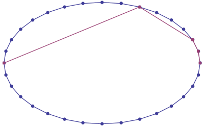
Figure 1: Illustration of the behavior of geometric scaling. The picture shows a polytope in $\mathds{R}^{2}$. Our initial point is the leftmost point and we maximize $c=(1,0)$ (i.e., the maximum is the rightmost point). A worst-case augmentation oracle might give the point with smallest improvement, which is always an adjacent vertex or jump between bottom and top. Standard augmentation with such a malicious worst-case oracle would now force us to visit either each point on the upper or lower path. Geometric scaling constructs shortcuts by controlling the objective function, leading to significant speed-ups.

As with bit scaling and MRA, Algorithm 3 also requires only polynomially many augmentations with respect to the encoding length. First we bound the number of augmentations required per scaling phase.

Lemma 3.12 (Schulz and Weismantel (2002)).

Let $P=\left\{{x\in\mathds{R}^{n}}\,\middle|\,{Ax=b,\,l\leq x\leq u}\right\}$, let $\rho$ be the potential function from Lemma 3.6, and let $x^{0}\in P\cap\mathds{Z}^{n}$ be an integer feasible solution. Then Algorithm 3 computes at most $4n$ approximate MRA directions between successive updates of $\mu$.

Proof.

Let $y^{0},y^{1},\dotsc$ be the points in $P$ visited by the algorithm during the scaling phase for a given $\mu$. In particular, $y^{0}$ is the current solution after the last update of $\mu$. By Observation 3.10, we have

$$\frac{c(x^{\star}-y^{0})}{\rho(y^{0},x^{\star}-y^{0})}\leq 2\mu,$$

where $x^{\star}$ is an integral optimal solution for the original problem. Now, consider any two consecutive iterates $y^{i}$ and $y^{i+1}$. By definition of Algorithm 3, the $c(y^{i+1}-y^{i})-\mu\cdot\rho(y^{i},y^{i+1}-y^{i})>0$ holds. Moreover, as the direction $y^{i+1}-y^{i}$ is exhaustive, using Lemma 3.6, we have

$$c(y^{i+1}-y^{i}) >\mu\cdot\rho(y^{i},y^{i+1}-y^{i})\geq\frac{\mu}{2}\geq\frac{1}{4}\frac{c(x^{\star}-y^{0})}{\rho(y^{0},x^{\star}-y^{0})}\geq\frac{1}{4n}c(x^{\star}-y^{0}),$$

hence we compute at most $4n$ approximate directions in each scaling phase. ∎

It is interesting to observe that in Lemma 3.12, in each scaling phase, we recover at least a $\tfrac{1}{4n}$ fraction of the improvement of the optimal direction $x^{\star}-y^{0}$ from the feasible solution $y^{0}$ at the beginning of the phase to the optimal solution $x^{\star}$. This is in contrast to Theorem 3.9, where the guaranteed improvement of $\tfrac{1}{2n}$ is with respect to two consecutive iterates only, i.e., we only guarantee to recover an $\tfrac{1}{2n}$ fraction of the improvement of $x^{\star}-y^{i-1}$, if we are in iteration $i$, which is potentially smaller than the one from direction $x^{\star}-y^{0}$.

We will now establish a bound on the number of required approximate MRA directions, which slightly improves the bound in Schulz and Weismantel (2002) by a $\log n$ factor. The key insight is that we can combine Observation 3.11 with Observation 3.10, to switch from the multiplicative regime to the additive regime, simply counting the remaining improvement steps.

Theorem 3.13 (Improved bound for geometric scaling).

Let $P=\left\{{x\in\mathds{R}^{n}}\,\middle|\,{Ax=b,\,l\leq x\leq u}\right\}$, let $\rho$ be the potential function from Lemma 3.6, and let $x^{0}\in P\cap\mathds{Z}^{n}$ be an integer feasible solution. Then Algorithm 3 solves the optimization problem $\max\left\{{cx}\,\middle|\,{x\in P\cap\mathds{Z}^{n}}\right\}$ with at most $O({n\log(C(U-L))})$ computations of approximate MRA directions.

Proof.

The algorithm initializes with $\mu=2C(U-L)$. Hence after $\lceil{\log(C(U-L))}\rceil+1$ updates of $\mu$, we have $\mu\leq 1$, and by Lemma 3.12 have computed at most $4n(\lceil{\log(C(U-L))}\rceil+1)$ approximate MRA directions in total. Let $\tilde{x}$ be the last solution computed by the algorithm in these first $\lceil{\log(C(U-L))}\rceil+1$ scaling phases.

We now switch to the additive regime and simply count the number of remaining improvements that are possible. As $\mu\leq 1$, Observation 3.10 implies

$$c(x^{\star}-\tilde{x})\leq\mu\cdot\rho(\tilde{x},x^{\star}-\tilde{x})\leq n,$$

where $x^{\star}$ is an integral optimal solution with respect to $c$. Since all data is integral and by Observation 3.11, every approximate MRA direction leads to an improvement of the objective function by at least $1$. It follows that no more than $n$ solutions may be generated before obtaining a solution with cost $cx^{\star}$. Hence the algorithm terminates after computing at most $4n(\lceil{\log(C(U-L))}\rceil+1)+n$ approximate MRA directions. ∎

Remark 3.14 (Oracle calls vs. approximate MRA directions).

In Theorem 3.13 and elsewhere we count the number of approximate MRA directions that we compute. That is slightly different than counting the number of calls to an approximate MRA oracle: we do not count the number of calls for which no approximate MRA direction exist for a given scaling factor $\mu$ and where $\mu$ is rescaled. However, note that this number of calls is dominated by the number of calls which do return improving directions. For example in Theorem 3.13, in the last phase where $\mu\leq 1$, we rescale at most $O(\log n)=o(n)$ times until $\mu<1/n$. In fact, all our results also hold (up to constant factors) if we consider the number of oracle calls rather than approximate MRA directions.

Note that the bound in Theorem 3.13 is stronger than the one given in Theorem 3.9 for Algorithm 2. In fact, the above result implies the same worst-case bound for Algorithm 2: As Algorithm 3 may use a ratio-maximizing direction in each step, Algorithm 2 inherits any worst-case upper bounds proven for Algorithm 3. Thus we obtain the following improvement:

Corollary 3.15 (Improved bound for MRA).

Let $P=\left\{{x\in\mathds{R}^{n}}\,\middle|\,{Ax=b,\,l\leq x\leq u}\right\}$, $\rho$ be the potential function from Lemma 3.6, and let $x^{0}\in P\cap\mathds{Z}^{n}$. Then Algorithm 2 solves the optimization problem $\max\left\{{cx}\,\middle|\,{x\in P\cap\mathds{Z}^{n}}\right\}$ with at most $O({n\log(C(U-L))})$ computations of an MRA direction.

Moreover, in the case of 0/1 polytopes where the description of the LP relaxation is in equality form, we obtain:

Corollary 3.16 (Worst-case performance for 0/1 polytopes).

Let $P=\left\{{x\in\mathds{R}^{n}}\,\middle|\,{Ax=b,\,0\leq x\leq\mathds{1}}\right\}$, $\rho$ be the potential function from Lemma 3.6, and let $x^{0}\in P\cap\{0,1\}^{n}$. Then Algorithms 2 and 3 both solve the optimization problem $\max\left\{{cx}\,\middle|\,{x\in P\cap\{0,1\}^{n}}\right\}$ with at most $O({n\log C})$ augmentations.

3.3 Geometric scaling for arbitrary polytopes in the 0/1 cube

We will now briefly explain how the setup from above can be changed in the case of polytopes $P=\left\{x\mid Ax\leq b\right\}\subseteq[0,1]^{n}$, i.e., not requiring equality form. Clearly, $P$ can be written in equality form by adding slack variables. This, however, changes the ambient dimension, which affects all the bounds above. Moreover, slack variables do not necessarily have to be 0/1 variables, complicating things further. Thus, we present a tailored analysis for problems in the above form with a particular potential function.

The following observation is crucial:

Observation 3.17 (Exhaustiveness for 0/1 polytopes).

Every 0/1 solution $x\in P$ is a vertex of $P$, and, in particular, for each coordinate either $0\leq x$ or $x\geq\mathds{1}$ is tight, so that any direction $0\neq z\in\left\{-1,0,1\right\}^{n}$ is always exhaustive. For the potential function $\rho(x,z)\coloneqq\left\lVert z\right\rVert_{1}$, clearly $\rho(x,z)\leq n$, and $\rho(x,z)\geq 1$ whenever $z\neq 0$. Moreover, we do not need homogeneity, as no scaling of directions is required.

We obtain the following lemma with a proof essentially identical to the one for Lemma 3.12.

Lemma 3.18.

Let $P=\left\{{x\in\mathds{R}^{n}}\,\middle|\,{Ax\leq b,\,0\leq x\leq\mathds{1}}\right\}$, let $\rho(x,z)=\left\lVert z\right\rVert_{1}$, and let $x^{0}\in P\cap\left\{0,1\right\}^{n}$ be a feasible 0/1 solution. Then Algorithm 3 computes at most $2n$ approximate MRA directions between successive updates of $\mu$.

Proof.

The beginning of the proof is as in Lemma 3.12, but now two consecutive iterates $y^{i},y^{i+1}$ within a scaling phase satisfy

$$c(y^{i+1}-y^{i}) \geq\mu\cdot\rho(y^{i},y^{i+1}-y^{i})\geq\mu\geq\frac{1}{2}\frac{c(x^{\star}-y^{0})}{\rho(y^{0},x^{\star}-y^{0})}\geq\frac{1}{2n}c(x^{\star}-y^{0}),$$

by Observation 3.17, where $x^{\star}$ is an integral optimal solution with respect to $c$. Hence at most $2n$ approximate MRA directions are computed in each scaling phase. ∎

With this lemma we obtain the following version of Theorem 3.13 for arbitrary polytopes $P\subseteq[0,1]^{n}$. The proof follows exactly as in Theorem 3.13, but with Lemma 3.18 playing the role of Lemma 3.12.

Theorem 3.19.

Let $P=\left\{{x\in\mathds{R}^{n}}\,\middle|\,{Ax\leq b,\,0\leq x\leq\mathds{1}}\right\}$, let $\rho(x,z)=\left\lVert z\right\rVert_{1}$, and let $x^{0}\in P\cap\left\{0,1\right\}^{n}$ be a feasible 0/1 solution. Then Algorithm 3 solves the optimization problem $\max\left\{{cx}\,\middle|\,{x\in P\cap\{0,1\}^{n}}\right\}$ with at most $O({n\log C})$ computations of approximate MRA directions.

In particular, the computation of the approximate MRA direction can be performed with a single call to an augmentation oracle as the resulting program with $\left\lVert\cdot\right\rVert_{1}$ as potential function can be phrased as an integer program. Thus, bit scaling and geometric scaling require essentially the same number of computations of augmenting steps (see Lemma 3.1). The following is a generalization of Corollary 3.16 in the case of $P\subseteq[0,1]^{n}$.

Corollary 3.20.

Let $P=\left\{{x\in\mathds{R}^{n}}\,\middle|\,{Ax\leq b,\,0\leq x\leq\mathds{1}}\right\}\subseteq[0,1]^{n}$ be a polytope and consider the potential function $\rho(x,z)\coloneqq\left\lVert z\right\rVert_{1}$. Let $x^{0}\in P\cap\{0,1\}^{n}$ be an arbitrary integral solution. Then Algorithms 2 and 3 both solve the optimization problem $\max\left\{{cx}\,\middle|\,{x\in P\cap\{0,1\}^{n}}\right\}$ with at most $O({n\log C})$ augmentations.

We will now give an intuition for the result above. In fact, it turns out that the geometric scaling algorithm (Algorithm 3) and bit scaling (Algorithm 1) are closely related:

Remark 3.21 (Relation between bit scaling and geometric scaling).

Observe that the potential function from Lemma 3.6 is equivalent to the potential function $\rho(\tilde{x},x-\tilde{x})\coloneqq\lvert{\operatorname{supp}(x-\tilde{x})}\rvert$ in the 0/1 case, provided we consider only feasible directions. Now consider a polytope $P\subseteq[0,1]^{n}$, an integral objective function $c\in\mathds{Z}^{n}_{+}$ (which we can assume to be nonnegative by flipping), an integer feasible point $\tilde{x}\in P\cap\left\{0,1\right\}^{n}$, and $\mu=2^{\ell}$ for some $\ell\in\mathds{N}$. In Algorithm 3 we search for a direction $z$ defined by $z=x-\tilde{x}$, where $x\in P$ is integer feasible so that

$$c(x-\tilde{x})-\mu\,\lvert{\operatorname{supp}(x-\tilde{x})}\rvert>0.$$

If we would now pick any coordinate $j\in[n]$, then the above stipulates that it is only beneficial to deviate from the $\tilde{x}_{j}$ value if $c_{j}>2^{\ell}$. Writing $c=c^{1}+c^{0}$ with $c^{1}\coloneqq\lfloor{c/2^{\ell}}\rfloor\cdot 2^{\ell}$ and $c^{0}\coloneqq c-c^{1}$, we obtain

$$c^{1}(x-\tilde{x})+\underbrace{c^{0}(x-\tilde{x})-2^{\ell}\,\lvert{\operatorname{supp}(x-\tilde{x})}\rvert}_{\leq 0}>0.$$

Hence, $c^{1}(x-x_{0})>0$ is a necessary condition. Although this condition does not guarantee an improvement over $\tfrac{cx}{\rho(\tilde{x},x-\tilde{x})}$, in each phase at most $n$ augmentation steps are necessary (see the analysis in the proof of Lemma 3.1), leading virtually to the same overall running time as for Algorithm 3, however with the additional simplification of not explicitly having to consider the potential.

3.4 Improved bounds for structured 0/1 polytopes

When proving worst-case bounds for both bit scaling and geometric scaling, a crucial element is the $O({n})$ bound on the number of improvements made per scaling phase. In the case of bit scaling, this bound is due to the number of positive entries in the vector $x-\tilde{x}$ being at most $n$ for any integral point $x$, $\tilde{x}\in P$. For geometric scaling, the bound arises from potential function values. In particular, the potential $\rho(x,z)\coloneqq\left\lVert z\right\rVert_{1}$ is bounded from above by $n$. If this bound can be reduced for special polytopes, it would have direct consequences for worst-case bounds of either algorithm.

One condition that guarantees such a reduction is the following: Let $P\subseteq[0,1]^{n}$ be a polytope, and suppose there exists some function $f:\mathds{Z}_{+}\rightarrow\mathds{Z}_{+}$ such that every integral point $x\in P$ has no more than $f(n)$ nonzero entries. In particular we are hoping for an $o(n)$ function, such as $\sqrt{n}$ or $\log n$. We then obtain the following improved worst-case bounds for both bit scaling and geometric scaling.

Theorem 3.22.

Let $c\in\mathds{R}^{n}$ be a cost vector, $P\subseteq[0,1]^{n}$ a polytope, and let the potential function $\rho$ be given as $\rho(x,z)\coloneqq\left\lVert z\right\rVert_{1}$. Suppose there exists a function $f:\mathds{Z}_{+}\to\mathds{Z}_{+}$ such that every integral point $x\in P$ has at most $f(n)$ nonzero entries. Then, given an initial solution $x^{0}\in P$, Algorithms 1 and 3 solve the optimization problem $\max\left\{{cx}\,\middle|\,{x\in P\cap\mathds{Z}^{n}}\right\}$ after $O({f(n)\log C})$ augmentations.

Proof.

For Algorithm 1 the proof follows as for Lemma 3.1: suppose $x^{\mu}\in P$ optimizes $c^{\mu}=\lfloor{c/\mu}\rfloor$ over $P$, and we move to the next scaling phase (dividing $\mu$ by 2) in which we optimize over $c^{\prime}=2c^{\mu}+\tilde{c}$ for some $\tilde{c}\in\{0,1\}^{n}$. If we take $x^{\prime}$ to be an optimal solution with respect to $c^{\prime}$, we have

$$c^{\prime}(x^{\prime}-x^{\mu})=\underbrace{2c^{\mu}(x^{\prime}-x^{\mu})}_{\leq 0}+\underbrace{\tilde{c}(x^{\prime}-x^{\mu})}_{\leq 2\,f(n)}\leq 2f(n),$$

since the direction $x^{\prime}-x^{\mu}\in\{-1,0,1\}^{n}$ has at most $2\,f(n)$ positive entries. Hence, no more than $2f(n)$ improvements can be made in any of the $\lceil{\log C}\rceil+1$ scaling phases.

In the case of Algorithm 3, we know that $\rho$ is bounded above by $2f(n)$. From this point forward, the proof follows exactly as for Theorem 3.13, with requiring in total at most $8f(n)(\lceil{\log(C)}\rceil+1)+2f(n)$ approximate MRA directions. ∎

Many well-studied polytopes satisfy the structural constraint from Theorem 3.22, especially those arising from graph-theoretic problems. For example, take the traveling salesman polytope $P\subseteq[0,1]^{E}$ on the complete graph with $k$ nodes and $\left\lvert E\right\rvert=\binom{k}{2}$ edges. Even though the polytope is contained in a space of ambient dimension $\binom{k}{2}$, its integral points (corresponding to tours on the graph) contain exactly $k$ nonzero entries, spanning a low dimensional subspace. Hence optimizing over $P$ using either Algorithm 1 or Algorithm 3 can be done in $O({k\log C})$ augmentations, a factor-$k$ improvement over the general $O({k^{2}\log C})$ upper bound. Similar statements hold for the case of maximum weight matchings on a complete graph.

4 Worst-case example for bit scaling

We will now show that the upper bound in Lemma 3.1, on the number of augmentations necessary for bit scaling, is tight. For this we provide a family of polytopes $P_{n}\subseteq[0,1]^{n}$ and cost functions $c^{p}$ so that the bit scaling method needs $\Omega(n\log\left\lVert c^{p}\right\rVert_{\infty})$ augmentation steps in the worst case.

Each instance of this family is parametrized by two numbers, namely $k\in\mathds{Z}_{+}$, which dictates the dimension $n\coloneqq 8k-2$ of the cube $[0,1]^{n}$, and $p\in\mathds{Z}_{+}$, which controls how the objective function $c^{p}$ is built, and, by construction, the number $p$ of bit scaling phases that will be required to solve the instance.

4.1 Construction of the polytope

The polytope $P_{n}\subseteq[0,1]^{n}$ will be of the form

$$P_{n}=\operatorname{conv}\left(\left\{y^{1},\dots,y^{2k}\right\}\right),$$

where the vectors $y^{j}\in\{0,1\}^{n}$ are defined in terms of vectors $y^{j,1}\in\{0,1\}^{k-1},y^{j,2}\in\{0,1\}^{k-1},y^{j,3}\in\{0,1\}^{3k}$, and $y^{j,4}\in\{0,1\}^{3k}$. With these four families of vectors defined, the full vector $y^{j}$ is given by

$$y^{j}\coloneqq\begin{pmatrix}y^{j,1}\\ y^{j,2}\\ y^{j,3}\\ y^{j,4}\end{pmatrix}\qquad\text{or equivalently}\qquad y^{j}_{i}\coloneqq\begin{cases}y^{j,1}_{i}&\text{for }i\in\{1,\dots,k-1\},\\ y^{j,2}_{i-k+1}&\text{for }i\in\{k,\dots,2k-2\},\\ y^{j,3}_{i-2k+2}&\text{for }i\in\{2k-1,\dots,5k-2\},\\ y^{j,4}_{i-5k+2}&\text{for }i\in\{5k-1,\dots,8k-2\}.\end{cases}$$

The parts $y^{j,1},y^{j,2}$ are defined in two batches. For the first batch with $j\in\left\{1,\dots,k\right\}$, we define

$$y^{j,1}_{i}\coloneqq\begin{cases}1&\text{if }i\geq j,\\ 0&\text{otherwise},\end{cases}\quad\quad y^{j,2}_{i}\coloneqq\begin{cases}1&\text{if }i<j,\\ 0&\text{otherwise}\end{cases}\quad\text{ for }i=1,\dots,k-1.$$

For the second batch with $j\in\left\{k+1,\dots,2k\right\}$, we define

$$y^{j,1}_{i}\coloneqq\begin{cases}1&\text{if }i\geq j-k,\\ 0&\text{otherwise},\end{cases}\quad\quad y^{j,2}_{i}\coloneqq\begin{cases}1&\text{if }i<j-k,\\ 0&\text{otherwise},\end{cases}\quad\text{ for }i=1,\dots,k-1.$$

We define $y^{j,3},y^{j,4}$ with $j\in\left\{1,\dots,2k\right\}$ as follows

$$y^{j,3}_{i}\coloneqq\begin{cases}1&\text{if }j\leq k,\\ 0&\text{otherwise},\end{cases}\quad\quad y^{j,4}_{i}\coloneqq\begin{cases}1&\text{if }j>k,\\ 0&\text{otherwise},\end{cases}\quad\text{ for }i=1,\dots,3k.$$

See Figure 2 for an illustration.

4.2 Construction of the cost vector

The cost vector is defined inductively, keeping the mechanics of the bit scaling procedure in mind. We first define $c^{0}\coloneqq 0$, and for $\ell=1,\dots,p$, we build $c^{\ell}=2c^{\ell-1}+d^{\ell}$, for some vector $d^{\ell}\in\{0,1\}^{n}$ to be specified. We will find it convenient to construct $d^{\ell}=(d^{\ell,1},d^{\ell,2},d^{\ell,3},d^{\ell,4})$ in terms of vectors $d^{\ell,1},d^{\ell,2},d^{\ell,3}$, and $d^{\ell,4}$ in the same manner as we did for the points $y^{j}$.

For $d^{1}\coloneqq c^{1}$, let

$$d^{1,1}\coloneqq\mathds{1},\quad\quad d^{1,2}\coloneqq 0,\quad\quad d^{1,3}_{i}\coloneqq\begin{cases}1&\text{if }i\leq k,\\ 0&\text{otherwise},\end{cases}\text{ for }i=1,\dots,3k,\quad\quad d^{1,4}\coloneqq 0.$$

For $\ell\geq 2$, we set

$$d^{\ell,1}\coloneqq 0,\quad\quad d^{\ell,2}\coloneqq\mathds{1},\quad\quad d^{\ell,3}\coloneqq\begin{cases}\mathds{1}&\text{if }\ell\text{ is odd},\\ 0&\text{otherwise},\end{cases}\quad\quad d^{\ell,4}\coloneqq\begin{cases}\mathds{1}&\text{if }\ell\text{ is even},\\ 0&\text{otherwise}.\end{cases}$$

In particular, after the first scaling phase, the contribution of the first $2(k-1)$ coordinates is the same for all $y^{j}$. In fact, we use the first $2(k-1)$ coordinates for the improvements steps within a scaling phase and the last $6k$ coordinates to switch between the phases; this will become clear soon. Note that for each $\ell>1$, $\log\left\lVert c^{\ell}\right\rVert_{\infty}\in\Theta(\ell)$.

4.3 Lower bound on the number of augmentations

We will now derive a lower bound on the worst-case number of augmentations computed by the bit scaling algorithm when applied to a polytope $P_{n}$ and cost vector $c^{p}$ as defined in Section 4.1 and 4.2, respectively. We depict the overall structure of the construction in Figure 2, describing the points $y^{j}$ and the “layers” $d^{\ell}$ of the cost function. Note how the columns in Figure 2 are divided into four segments. These four segments correspond to the four families of vectors used in defining $y^{j}$ and $d^{\ell}$. For example, the first group of columns in the $y^{j}$ row depict the vector $y^{j,1}$, the second group of columns depict $y^{j,2}$, and so on.

$$\begin{array}[]{c|ccccc|ccccc|cccc|cccc}\hline\cr\hline\cr&\lx@intercol\hfil y^{j,1}\hfil\lx@intercol\vrule\lx@intercol&\lx@intercol\hfil y^{j,2}\hfil\lx@intercol\vrule\lx@intercol&\lx@intercol\hfil y^{j,3}\hfil\lx@intercol\vrule\lx@intercol&\lx@intercol\hfil y^{j,4}\hfil\lx@intercol\\ \hline\cr&1&2&3&\cdots&k-1&1&2&3&\cdots&k-1&1&2&\cdots&3k&1&2&\cdots&3k\\ \hline\cr y^{1}&1&1&1&\cdots&1&0&0&0&\cdots&0&1&1&\cdots&1&0&0&\cdots&0\\ y^{2}&0&1&1&\cdots&1&1&0&0&\cdots&0&1&1&\cdots&1&0&0&\cdots&0\\ y^{3}&0&0&1&\cdots&1&1&1&0&\cdots&0&1&1&\cdots&1&0&0&\cdots&0\\ \vdots&\vdots&\vdots&\vdots&\ddots&\vdots&\vdots&\vdots&\vdots&\ddots&\vdots&\vdots&\vdots&\ddots&\vdots&\vdots&\vdots&\ddots&\vdots\\ y^{k}&0&0&0&\cdots&0&1&1&1&\cdots&1&1&1&\cdots&1&0&0&\cdots&0\\ \hline\cr y^{k+1}&1&1&1&\cdots&1&0&0&0&\cdots&0&0&0&\cdots&0&1&1&\cdots&1\\ y^{k+2}&0&1&1&\cdots&1&1&0&0&\cdots&0&0&0&\cdots&0&1&1&\cdots&1\\ y^{k+3}&0&0&1&\cdots&1&1&1&0&\cdots&0&0&0&\cdots&0&1&1&\cdots&1\\ \vdots&\vdots&\vdots&\vdots&\ddots&\vdots&\vdots&\vdots&\vdots&\ddots&\vdots&\vdots&\vdots&\ddots&\vdots&\vdots&\vdots&\ddots&\vdots\\ y^{2k}&0&0&0&\cdots&0&1&1&1&\cdots&1&0&0&\cdots&0&1&1&\cdots&1\\ \hline\cr d^{1}&1&1&1&\cdots&1&0&0&0&\cdots&0&d^{1,3}_{1}&d^{1,3}_{2}&\cdots&d^{1,3}_{3k}&0&0&\cdots&0\\ d^{2}&0&0&0&\cdots&0&1&1&1&\cdots&1&0&0&\cdots&0&1&1&\cdots&1\\ d^{3}&0&0&0&\cdots&0&1&1&1&\cdots&1&1&1&\cdots&1&0&0&\cdots&0\\ d^{4}&0&0&0&\cdots&0&1&1&1&\cdots&1&0&0&\cdots&0&1&1&\cdots&1\\ d^{5}&0&0&0&\cdots&0&1&1&1&\cdots&1&1&1&\cdots&1&0&0&\cdots&0\\ \vdots&\vdots&\vdots&\vdots&\vdots&\vdots&\vdots&\vdots&\vdots&\vdots&\vdots&\vdots&\vdots&\vdots&\vdots&\vdots&\vdots&\vdots&\vdots\\ \hline\cr\hline\cr\end{array}$$

Figure 2: Structure of $y^{j}$ and $d^{\ell}$; note that $d^{1,3}$ depends on $k$.

The essence of the proof is the following: within a scaling phase, the algorithm may move to any solution with an improving cost with respect to vector $\lfloor{c/\mu}\rfloor$ (recall that $\mu$ is the scaling factor), no matter the magnitude of the improvement. In our construction, no matter the choice of $k,\ell$, the bit scaling algorithm begins by optimizing over the cost vector $c^{1}$. The construction is such that $c^{1}y^{1}>c^{1}y^{2}>\dots>c^{1}y^{2k}$. Thus if the algorithm begins at initial solution $y^{2k}$, it may visit all of the $2k$ points in $P_{n}$, ending the initial phase at $y^{1}$.

In the second scaling phase, the algorithm optimizes over $c^{2}$. We will see that we have $c^{2}y^{1}<c^{2}y^{2k}<c^{2}y^{2k-1}<\dots<c^{2}y^{k+1}$. Thus, in this phase, the algorithm may take $k$ augmentation steps before finishing at point $y^{k+1}$. In the third augmentation phase, while optimizing over $c^{3}$, we similarly have $c^{3}y^{k+1}<c^{3}y^{k}<\dots<c^{3}y^{1}$, giving another possible $k$ augmentations within the phase.

The process continues in each subsequent scaling phase, with the algorithm having the opportunity to travel through each of the points $y^{2k},y^{2k-1},\dots,y^{k+1}$ in even phases, and $y^{k},y^{k-1},\dots,y^{1}$ in odd phases, as depicted in Figure 3. Since $k\approx n/8$, this implies a worst case $O({n})$ augmentations per scaling phase, meeting the upper bound from Lemma 3.1.

We now begin the formal proof. We will first show that in each phase $\ell$, the first $k$ points $y^{1},\dots,y^{k}$ are ordered in a decreasing fashion by the objective function $c^{\ell}$ and similar for the second $k$ points $y^{k+1},\dots,y^{2k}$. In a second step we will then link the two groups.

Lemma 4.1 (Decreasing order within each group).

Let $c^{\ell},y^{j}$ be constructed as above. For any $\ell\geq 1$ and $j\in\left\{1,\dots,k-1\right\}\cup\left\{k+1,\dots,2k-1\right\}$, we have

$$c^{\ell}y^{j}=c^{\ell}y^{j+1}+1.$$

Proof.

The proof is by induction on $\ell$, with base case $\ell=1$. For $j\in\{1,\dots,2k\}$, define $\alpha_{1,j}\coloneqq d^{1,3}y^{j,3}$. For $j\in\{1,\dots,2k\}$, we have

$$c^{1}y^{j}=d^{1}y^{j}=\underbrace{d^{1,1}y^{j,1}}_{=k-j}+\underbrace{d^{1,2}y^{j,2}}_{=0}+\underbrace{d^{1,3}y^{j,3}}_{=\alpha_{1,j}}+\underbrace{d^{1,4}y^{j,4}}_{=0}=k-j+\alpha_{1,j}.$$

By construction, we have $\alpha_{1,1}=\alpha_{1,2}=\dots=\alpha_{1,k}=1$ and $\alpha_{1,k+1}=\alpha_{1,k+2}=\dots=\alpha_{1,2k}=0$. Thus for $j\in\left\{1,\dots,k-1\right\}\cup\left\{k+1,\dots,2k-1\right\}$, we can establish

$$c^{1}y^{j}-c^{1}y^{j+1}=k-j+\alpha_{1,j}-(k-(j+1)+\alpha_{1,j+1})=1,$$

as $\alpha_{1,j+1}=\alpha_{1,j}$.

Now assume $\ell\geq 2$. For $j\in\{1,\dots,k\}$ we can verify that

$$c^{\ell}y^{j} =2c^{\ell-1}y^{j}+d^{\ell}y^{j}$$

$$=2c^{\ell-1}y^{j}+\underbrace{d^{\ell,1}y^{j,1}}_{=0,\text{ as }d^{\ell,1}=0}+\underbrace{d^{\ell,2}y^{j,2}}_{=j-1}+\underbrace{d^{\ell,3}y^{j,3}}_{\eqqcolon\alpha_{\ell}}+\underbrace{d^{\ell,4}y^{j,4}}_{=0,\text{ as }y^{j,4}=0\text{ for }j\leq k}$$

$$=2c^{\ell-1}y^{j}+(j-1)+\alpha_{\ell},$$

where $\alpha_{\ell}=3k$ if $\ell$ is odd, and otherwise $\alpha_{\ell}=0$. Thus, for $j\in\left\{1,\dots,k-1\right\}$ we have

$$c^{\ell}y^{j}-c^{\ell}y^{j+1} =2c^{\ell-1}y^{j}+j-1+\alpha_{\ell}-(2c^{\ell-1}y^{j+1}+j+\alpha_{\ell})$$

$$=2(\underbrace{c^{\ell-1}y^{j}-c^{\ell-1}y^{j+1}}_{=1,\text{ by induction}})-1=1.$$

We can do a similar analysis for $\ell\geq 2$ and $j\in\left\{k+1,\dots,2k\right\}$:

$$c^{\ell}y^{j} =2c^{\ell-1}y^{j}+d^{\ell}y^{j}$$

$$=2c^{\ell-1}y^{j}+\underbrace{d^{\ell,1}y^{j,1}}_{=0,\text{ as }d^{\ell,1}=0}+\underbrace{d^{\ell,2}y^{j,2}}_{=j-1}+\underbrace{d^{\ell,3}y^{j,3}}_{=0,\text{ as }y^{j,3}=0\text{ for }j\geq k+1}+\underbrace{d^{\ell,4}y^{j,4}}_{\eqqcolon\beta_{\ell}}$$

$$=2c^{\ell-1}y^{j}+(j-1)+\beta_{\ell},$$

where $\beta_{\ell}=3k$ if $\ell$ is even, and $\beta_{\ell}=0$ otherwise . As before we obtain that for $j=k+1,\dots,2k-1$, $c^{\ell}y^{j}-c^{\ell}y^{j+1}=1$ holds. ∎

Note that in the above argument the values of $d^{\ell,3}$, $d^{\ell,4}$ are irrelevant as they are eliminated in the difference of two consecutive points. However, they will become important as they enable the switching between and linking of the two groups $\{y^{1},\dots,y^{k}\}$ and $\{y^{k+1},\dots,y^{2k}\}$ as we will show now. To this end we prove the following lemma:

Lemma 4.2 (Decreasing intergroup ordering).

For any $\ell\geq 1$, if $\ell$ is odd then $c^{\ell}y^{k}=c^{\ell}y^{k+1}+1$, and if $\ell$ is even then $c^{\ell}y^{2k}=c^{\ell}y^{1}+1$.

Proof.

The proof is by alternating induction on the odd and even case. First observe that $c^{1}y^{k}=c^{1}y^{k+1}+1$, which will be the start of our induction for the odd case:

$$c^{1}y^{k}-c^{1}y^{k+1} =\underbrace{d^{1,1}(y^{k,1}-y^{k+1,1})}_{=-(k-1)}+\underbrace{d^{1,2}(y^{k,2}-y^{k+1,2})}_{=0}+\underbrace{d^{1,3}(y^{k,3}-y^{k+1,3})}_{=k}+\underbrace{d^{1,4}(y^{k,4}-y^{k+1,4})}_{=0}=1.$$

First, let $\ell\geq 1$ be even and suppose $c^{\ell-1}y^{k}=c^{\ell-1}y^{k+1}+1$, which is satisfied in the case $\ell=2$ by the above. Then, repeated application of Lemma 4.1 yields $c^{\ell-1}y^{1}=c^{\ell-1}y^{2k}+2k-1$. Moreover, we have

$$c^{\ell}y^{1} =2c^{\ell-1}y^{1}+d^{\ell}y^{1}=2c^{\ell-1}y^{1}+\underbrace{d^{\ell,1}y^{1,1}}_{=0,\text{ as $\ell>1$}}+\underbrace{d^{\ell,2}y^{1,2}}_{=0,\text{ as $y^{1,2}=0$}}+\underbrace{d^{\ell,3}y^{1,3}}_{=0,\text{ as $\ell$ even }}+\underbrace{d^{\ell,4}y^{1,4}}_{=0,\text{ as $y^{1,4}=0$}}=2c^{\ell-1}y^{1},$$

and

$$c^{\ell}y^{2k} =2c^{\ell-1}y^{2k}+d^{\ell}y^{2k}=2c^{\ell-1}y^{2k}+\underbrace{d^{\ell,1}y^{2k,1}}_{=0,\text{ as $\ell>1$}}+\underbrace{d^{\ell,2}y^{2k,2}}_{=k-1}+\underbrace{d^{\ell,3}y^{2k,3}}_{=0,\text{ as $\ell$ even }}+\underbrace{d^{\ell,4}y^{2k,4}}_{=3k}$$

$$=2c^{\ell-1}y^{2k}+(k-1)+3k=2c^{\ell-1}y^{2k}+4k-1.$$

Thus, we obtain for the difference

$$c^{\ell}y^{2k}-c^{\ell}y^{1} =2c^{\ell-1}y^{2k}+4k-1-2c^{\ell-1}y^{1}$$

$$=2(\underbrace{c^{\ell-1}y^{2k}-c^{\ell-1}y^{1}}_{=1-2k,\text{ from above}})+4k-1=2(1-2k)+4k-1=1.$$

Now we consider the case where $\ell$ is odd, which is similar to the one above. Assume that $c^{\ell-1}y^{2k}=c^{\ell-1}y^{1}+1$, which we now know to hold for $\ell=3$ by means of the argument for $\ell$ even case from above. Then, applying Lemma 4.1 in increasing and decreasing direction, we obtain $c^{\ell-1}y^{k}+2k-1=c^{\ell-1}y^{k+1}$. We will show that $c^{\ell}y^{k}=c^{\ell}y^{k+1}+1$. We have

$$c^{\ell}y^{k}=2c^{\ell-1}y^{k}+\underbrace{d^{\ell,1}y^{k,1}}_{=0}+\underbrace{d^{\ell,2}y^{k,2}}_{=k-1}+\underbrace{d^{\ell,3}y^{k,3}}_{=3k}+\underbrace{d^{\ell,4}y^{k,4}}_{=0}=2c^{\ell-1}y^{k}+4k-1$$

and

$$c^{\ell}y^{k+1}=2c^{\ell-1}y^{k+1}+\underbrace{d^{\ell,1}y^{k+1,1}}_{=0}+\underbrace{d^{\ell,2}y^{k+1,2}}_{=0}+\underbrace{d^{\ell,3}y^{k+1,3}}_{=0}+\underbrace{d^{\ell,4}y^{k+1,4}}_{=0}=2c^{\ell-1}y^{k+1},$$

so that

$$c^{\ell}y^{k}-c^{\ell}y^{k+1}=2(\underbrace{c^{\ell-1}y^{k}-c^{\ell-1}y^{k+1}}_{=1-2k})+4k-1=1.$$

With these last two lemmas in hand, we are ready to prove the worst-case lower bound. The proof describes the possible behavior of the bit scaling algorithm when given a polytope $P_{n}$ and cost vector $c^{p}$, as depicted in Figure 3. The $\Omega(n\log\left\lVert c^{p}\right\rVert_{\infty})$ lower bound proven here meets the upper bound established in Lemma 3.1, implying that the analysis is tight.

Figure 3: Points visited by the bit scaling algorithm in the worst case. Black arcs follow via Lemma 4.1, red arcs via Lemma 4.2.

Theorem 4.3.

Choose $k\geq 1$ and set $n\coloneqq 8k-2$. Let $P_{n}=\operatorname{conv}\left(\left\{y^{1},\dots,y^{2k}\right\}\right)$ be the polytope and $c^{p}$ for some $p\geq 1$ the objective function as constructed above. Then the bit scaling algorithm optimizing $c^{p}$ over $P_{n}$ requires $\Omega(n\log\left\lVert c^{p}\right\rVert_{\infty})$ augmentation steps in the worst case.

Proof.

By construction of $c^{p}$, the bit scaling algorithm optimizes over $c^{1},c^{2},\dots,c^{p}$ in successive scaling phases. The algorithm begins by optimizing over $c^{1}$. By Lemmas 4.1 and 4.2 we have

$$c^{1}y^{2k}<c^{1}y^{2k-1}<\cdots<c^{1}y^{1}.$$

Since an augmentation step moves to any point with improving cost, the algorithm may be forced to visit all $2k$ points when optimizing over $c^{1}$.

For $\ell\geq 2$ and $\ell$ even, $y^{1}$ maximizes $c^{\ell-1}$ over $P_{n}$ and

$$c^{\ell}y^{1}<c^{\ell}y^{2k}<c^{\ell}y^{2k-1}<\cdots<c^{\ell}y^{k+1},$$

so the bit scaling algorithm may visit all $k$ points in $\left\{y^{k+1},\dots,y^{2k}\right\}$ in the $\ell$th scaling phase. Similarly, for $\ell\geq 2$ and $\ell$ odd, $y^{k+1}$ maximizes $c^{\ell-1}$ over $P_{n}$ and

$$c^{\ell}y^{k+1}<c^{\ell}y^{k}<c^{\ell}y^{k-1}<\cdots<c^{\ell}y^{1},$$

so the algorithm may visit all $k$ points in $\left\{y^{1},\dots,y^{k}\right\}$. Thus, for $\ell\in\{1,\dots,p\}$, at least $k$ augmentations may be necessary to optimize over $c^{\ell}$. As $p=\lceil{\log\left\lVert c^{p}\right\rVert_{\infty}}\rceil$, this gives a total number of (at least)

$$k\lceil{\log\left\lVert c^{p}\right\rVert_{\infty}}\rceil=\frac{n+2}{8}\lceil{\log\left\lVert c^{p}\right\rVert_{\infty}}\rceil\in\Omega(n\log\left\lVert c^{p}\right\rVert_{\infty})$$

augmentations necessary over the entire algorithm. ∎

Observe that in the example we have constructed above, we revisit the points $y^{j}$ several times, which leads to the high worst-case number of augmentations. However, given the same polytope/cost vector pair $(P_{n},c^{p})$, geometric scaling behaves differently. In particular, as shown in Observation 3.11, the geometric scaling algorithm never revisits a point. Thus the number of augmentations necessary for geometric scaling is bounded by the number of vertices of $P_{n}$, which is $O({n})$. With a suitable choice of $p$ (recall $\log\left\lVert c^{p}\right\rVert_{\infty}\approx p$), the number of augmentations calculated by the two methods can have an arbitrarily high difference. We thus have the following corollary.

Corollary 4.4.

For any $p\geq 1$, there exists a polytope $P\subseteq[0,1]^{n}$ with $n=8k+2$, $k\in\mathds{Z}_{>0}$ and an objective function $c=c^{p}$, so that bit scaling computes $\Omega(n\log\left\lVert c^{p}\right\rVert_{\infty})=\Omega(np)$ augmenting directions in the worst case, while geometric scaling needs $O({n})$ augmenting directions. In particular, the relative difference can be made arbitrarily large by choosing $p$ appropriately.

Theorem 4.3 is particularly interesting as it shows that the number of required augmentations for the bit scaling algorithm is unbounded for 0/1 polytopes. On the other hand, the rounding scheme of Frank and Tardos (1987) can be used to turn an arbitrary $c\in\mathds{Q}^{n}$ into a vector $\bar{c}\in\mathds{Z}^{n}$ with encoding length $O(n^{3})$ in time polynomial in $n$ and $\log\left\lVert c\right\rVert_{\infty}$ such that optimizing both vectors results in the same optimal solution. Thus, bit scaling requires at most $O(n^{4})$ augmentations in the worst-case with preprocessing of the objective function. We obtain the same worst-case bound on the number of augmentations for geometric scaling.

5 Implementation

We implemented the discussed algorithms bit scaling (Algorithm 1), MRA (Algorithm 2), and geometric scaling (Algorithm 3) in C using the framework SCIP, see Achterberg (2009); SCIP . We also implemented a simple augmentation algorithm (“augment”) that iteratively searches for augmenting directions. All methods run for arbitrary mixed-integer problems as described in the following sections. Generally, for each instance we run presolving and solve the root node, including cuts. We then start running the described algorithms, but keep all cuts and solutions found by heuristics so far, including those found during the augmentation iterations.

5.1 Solving the augmentation problems

The augmentation problem is solved as a MIP. In general, we add an objective cut $cx\geq cx^{k}+\delta$ with respect to the current objective $c$ and last feasible iteration point $x^{k}$. We use $\delta=\lceil{2\varepsilon\cdot\lvert{cx^{k}}\rvert}\rceil$ if the objective is integral, i.e., is guaranteed to yield integral values for all feasible solutions; we set $\delta=2\varepsilon\cdot\lvert{cx^{k}}\rvert$ otherwise. Here $\varepsilon=10^{-6}$ is the feasibility tolerance of SCIP. (The first solution is found without adding this constraint.) Note that continuous variables do not need to be treated differently, i.e., the approach works for arbitrary MIPs.

We then solve the MIP subproblem until we find an improving solution $x^{k+1}$. For any such solution, we try to exhaust the direction, by searching for the largest integral $\alpha$ such that $x^{k}+\alpha(x^{k+1}-x^{k})$ is feasible.

The search for improving solutions can be incomplete: We first solve the root node of the subproblem and check whether we found an improving solution. If yes, we use this solution as an augmentation direction. Otherwise, we continue to solve the MIP until we find any feasible solution. It often happens that soon after finding some feasible solution, further solutions are found, e.g., by so-called exchange heuristics like 1-opt or crossover. We therefore continue the solution process until for a fixed number of nodes no further improving solution is found or the problem has been solved (this is called a “stall node limit” in SCIP).

Note that the last iteration has to be solved to optimality in all algorithms.

5.2 Augment

For the basic augmentation method we proceed as follows: at each iteration with current best solution $x^{k}$, we add an objective cut. We then iteratively search for improving solutions until we prove infeasibility (in this case, $x^{k}$ is optimal) or hit the time limit. Note that we solve the same problem as the original with an additional constraint. Since this constraint does not cut off any better solution, the dual bound obtained in each subproblem is valid for the original.

5.3 Bit scaling

Algorithm 4 Bit Scaling Variant

Input: Feasible solution $x_{0}$
Output: Optimal solution for $\max\left\{{cx}\,\middle|\,{x\in P\cap\mathds{Z}^{n}}\right\}$

$\mu\leftarrow 2^{\lceil{\log C}\rceil}$

repeat

     set $c_{0}\leftarrow\lfloor{c/\mu}\rfloor$

     compute $x_{0}\in P$ integral with $c_{0}x_{0}=\max\left\{cx\mid x\in P_{I}\right\}$

     $\mu\leftarrow\mu/2$

until $\mu<1$

return $x_{0}$ $\triangleright$ return optimal solution

In the bit scaling Algorithm 1, at each iteration, the problem is solved with the scaled objective function under the additional constraint that a solution must improve on the current one. The scaling factor is changed if no improving solution exists. In Algorithm 4, there is no additional constraint, but the optimal solution is computed at each iteration, rather than an improving solution; therefore, the scaling factor changes at each iteration. We have implemented both algorithms, as well as a variant of Algorithm 4 with an improving constraint (similar to Algorithm 1). This may alter the behavior of the MIP solver, but not the behavior of the algorithm itself.

Let us now point out further implementation issues. At the beginning of the algorithms, the objective function is replaced with the scaled version. In practice, the coefficients of the objective function may not be integer. Thus, an additional scaling may be needed to make the objective integral. For the variants where an improving constraint is used, such a constraint is added at the beginning of an iteration if a feasible solution is known. Between two iterations, we compare the objective functions and only solve the next iteration if the vectors are not equal up to a factor. Depending on the algorithm, we solve the iteration problem to optimality or use an incomplete search, as explained above. A new scaling factor is computed before each new iteration if the solution of the current iteration is optimal for the current objective function (note that this is systematically the case for Algorithm 4 and its variant).

5.4 Geometric scaling

Geometric scaling is implemented as described in Algorithm 3, using the function

$$\rho(\tilde{x},x-\tilde{x})\coloneqq\left\lVert x-\tilde{x}\right\rVert_{1},$$ (2)

i.e., $\rho(\tilde{x},z)=\left\lVert z\right\rVert_{1}$. Note that for 0/1 problems this function is equal to $\lvert{\operatorname{supp}(x-\tilde{x})}\rvert$, which is a potential function, see Section 3.2. For general integer variables, $\rho$ does not fulfill Part 1 of Definition 3.5. We nevertheless use this function, since it induces sparsity, is easy to handle, and also can be used for the MRA algorithm (see Section 5.6). Note that for general integer variables, we need to add artificial (continuous) variables that model the positive and negative parts.

Deviating from Algorithm 3, we start with $\mu$ equal to the smallest power of 2 larger than the value of any previously found solution; moreover, we make sure that the value of $\mu$ is not larger than $10^{8}$. If the objective is not integral, we may need to solve one final problem, if $\mu<1/n$. For each found solution, we try to exhaust the direction as described above.

5.5 Primal heuristic based on geometric scaling

It will turn out in our computational results that geometric scaling in general performs quite well. This motivates the implementation of a primal heuristic based on it. This heuristic is activated during an ordinary branch-and-cut run after a primal solution was found and for a certain number of nodes (by default 200) no further solution was found. It then runs the geometric scaling algorithm, but with a node limit for the individual subproblems that depends on the current number of nodes $N$. By default, we use $\min\{500,\max\{5000,0.1\,N\}\}$. We also stop if the total number of nodes exceeds $0.6\,N$. In this way, the effort spent in this heuristic is limited, and one can still benefit from solutions found during the ordinary tree search.

5.6 MRA

The implementation of MRA (Algorithm 2) is based on $\rho(\tilde{x},x-\tilde{x})=\left\lVert x-\tilde{x}\right\rVert_{1}$, as well. Note that this function is convex in $x$. We then want to solve

$$\max\left\{\frac{c(x-\tilde{x})}{\rho(\tilde{x},x-\tilde{x})}\mid c(x-\tilde{x})>0,\;x\in P,\;x\text{ integral}\right\}$$

where $\tilde{x}$ is some feasible solution. To solve this fractional program, we introduce a parameter $\mu\geq 0$ and check whether $c(x-\tilde{x})\geq\mu\cdot\rho(\tilde{x},x-\tilde{x})$ by maximizing $c(x-\tilde{x})-\mu\cdot\rho(\tilde{x},x-\tilde{x})$, which is concave in $x$. We then perform a binary search over $\mu$, increasing $\mu$ if the objective value is positive and decreasing $\mu$ otherwise. To solve the inner optimization problem of maximizing $c(x-\tilde{x})-\mu\,\rho(\tilde{x},x-\tilde{x})$, we rewrite it as

$$\max\left\{cx-\tau\mid\tau\geq c\tilde{x}+\mu\cdot\rho(\tilde{x},x-\tilde{x}),\;c(x-\tilde{x})>0,\;x\in P,\;x\text{ integral}\right\}.$$

(Note that: $cx-\tau\leq cx-c\tilde{x}-\mu\cdot\rho(\tilde{x},x-\tilde{x})=c(x-\tilde{x})-\mu\cdot\rho(\tilde{x},x-\tilde{x})$ for all feasible $x$.)

We solve this problem by iteratively generating subgradients for the convex function

$$f_{\mu}(x)\coloneqq c\tilde{x}+\mu\cdot\rho(\tilde{x},x-\tilde{x}).$$

Its subdifferential is

$$\partial f_{\mu}(x)=c-\mu\,\partial\left\lVert\cdot\right\rVert_{1}(x-\tilde{x})=c-\mu\operatorname{sgn}(x-\tilde{x}),$$

where we define the set of vectors

$$\operatorname{sgn}(x)_{j}\coloneqq\begin{cases}\{1\}&\text{if }x_{j}>0\\ [-1,1]&\text{if }x_{j}=0\\ \{-1\}&\text{if }x_{j}<0\end{cases}\qquad\text{ for all }j=1,\dots,n.$$

For each subgradient $h\in\partial f_{\mu}(\tilde{x})$, we obtain the subgradient inequality

$$f_{\mu}(x)\geq f_{\mu}(\tilde{x})+h(x-\tilde{x}).$$

Assuming that we have generated subgradients $h^{1},\dots,h^{k}$ for points $x_{1},\dots,x_{k}$, we solve

$$\max\left\{cx-\tau\mid\tau\geq f_{\mu}(x_{i})+h^{i}(x-x_{i}),\;i=1,\dots,k,\;c(x-x_{0})>0,\;x\in P,\;x\text{ integral}\right\}.$$ (3)

Let the optimal solution be $x^{k+1}$. We then compute a subgradient at $x^{k+1}$ and check whether its subgradient inequality is violated. Note that each solution of (3) is a primal solution that can be stored and used for the original problem.

[In our implementation, we actually solve the minimization version

$$\min\left\{-cx+\tau\mid\tau-h^{i}x\geq f_{\mu}(x_{i})-h^{i}x_{i},\;i=1,\dots,k,\;c(x-x_{0})>0,\;x\in P,\;x\text{ integral}\right\},$$

for technical reasons.]

In the first iteration, the problem is unbounded, since $\tau$ is unbounded. We therefore start with $x^{0}$ (which is actually infeasible) and take the subgradient $h^{0}=c\in\partial f_{\mu}(x^{0})$. The inequality added to the optimization problem is then

$$\tau\geq cx^{0}+c(x-x^{0})=cx.$$

Thus, $\tau$ is bounded from below, if there exists a feasible $x\in P$, $c(x-x^{0})>0$, $x$ integral.

6 Computational results

The algorithms were tested on a Linux cluster with 3.2 GHz Intel i3 processors with 8 GB of main memory and 4 MB of cache, running a single process at a time. We use SCIP 3.2.0 and CPLEX 12.6.1 as the LP-solver. SCIP runs with default settings, except that we turn off the “components” presolver, since it would decompose the problem into several runs, making a comparison more difficult.

We use the following testsets:

MIPLIB2010

The 87 benchmark instances from MIPLIB 2010, see Koch et al. (2011).

LB

We use the testset of 29 instances from the “local branching” paper, see  Fischetti and Lodi (2003). This testset has also been used in Hansen et al. (2006). The latter paper also contains improved results, which we will use below.

QUBO

We use a testset of linearizations of 50 instances for quadratically unconstrained Boolean optimization (QUBO), see Dash (2013); Dash and Puget (2015).

In an online supplement, we present details of the computations described in the following. We will first discuss results on the MIPLIB2010 test set. As it turns out, augmentation methods do not help to solve these instances, essentially because they are too easy. We then consider the very hard testsets LB and QUBO. Here, it will turn out that augmentation methods significantly improve on the default settings and produce primal solutions of very good quality.

6.1 Testset MIPLIB 2010

Table 1: Aggregated results of the different algorithms on testset MIPLIB 2010 (1 hour time limit, 87 instances)

name	#nodes	time	#run	#best	#improv.	#subprob.	#phases	#exhaust	prim-$\int$
bitscale	20116.2	934.93	59	67	3.7	8.4	4.8	0.0	57.4
MRA	16434.8	1819.46	83	32	411.4	428.6	418.7	8.1	207.2
geometric	5628.8	1632.31	83	65	6.2	23.6	17.4	0.0	49.8
augment	14793.5	924.71	83	63	12.9	12.9	12.9	0.0	54.5
bitscale-classic	25086.0	1120.62	59	62	4.1	11.0	6.9	0.0	60.4
bitscale-noimprove	20343.4	918.31	60	69	4.2	8.8	4.6	0.0	56.7
bitscale-complete	26902.6	1070.71	59	59	2.0	6.6	4.6	0.0	103.5
geom-no $\ell_{1}$	6038.5	1651.26	83	65	6.4	23.6	17.2	0.0	49.5
geom-no cutoff	7648.7	2062.03	83	49	3.9	19.4	15.6	0.0	85.4
geom-8	8637.7	1313.55	83	69	5.7	12.8	7.1	0.0	40.7
geom-64	8680.9	1122.85	83	72	6.4	10.7	4.3	0.0	39.7
geom-256	8358.2	1128.40	83	69	7.1	10.9	3.7	0.0	39.7
geom-512	9895.4	1112.03	83	69	7.0	10.3	3.3	0.0	41.8
geom-1024	8392.5	1016.80	83	71	7.1	10.3	3.2	0.0	39.8
geom-heur	16858.8	741.52	68	71	1.3	33.6	32.4	0.0	30.4
geom-infer	21343.6	732.30	68	72	1.0	41.7	40.7	0.0	30.1
geom-heur-64	16158.0	683.18	68	73	1.7	9.9	8.1	0.0	29.3
default	15495.9	557.12	0	74	0.0	0.0	0.0	0.0	26.3

Table 1 shows a comparison of the four different augmentation methods and variants of these as well as for the default settings on the testset MIPLIB2010. In the table, “#nodes” and “time” give the shifted geometric means of the total number of nodes (including subproblems) and the time (in seconds), respectively. Column “#run” presents the number of instances for which an augmentation routine ran. Column “#best” refers to the number of times the best known primal solution value has been found. With respect to the augmentation methods, the columns “#improv.”, “#subprob.”, “#phases”, and “#exhaust” refer to the average number of times an improved primal solution has been found, the number of subproblems (MIPs) solved, the number of phases, and the number of exhausting directions found, respectively. The number of phases refers to the number of subproblems solved with the same value of $\mu$ for bit and geometric scaling (in this case, $\text{\#phases}+\text{\#improv}=\text{\#subprob}$); note that we count a possible search for the first primal solution as one phase. For MRA, we count each outer iteration as a phase; thus, the number of phases equals the number of Benders problems (1) solved. For augment, the number of phases equals the number of improving solutions and the number of subproblems.

Finally, the last column gives the primal integral, see Berthold (2013). The primal integral is the value we obtain by integrating the gap between the current primal and best primal bound over time. Thus, a smaller primal integral indicates a higher solution quality over time.

We can draw several conclusions from these experiments:

General Observations

Among the 87 instances, four were solved before the end of the root node and no augmentation routine was applied.

The number of phases and subproblems is usually below 30, with the exception of MRA, which needs a larger number of phases and subproblems. Thus, it seems that in practice no long series of augmentation steps occur, but as the example of MRA shows, this would in principle be possible. Note, however, that the numbers are significantly smaller than the theoretical bounds.

The goal of the table is to illustrate the behavior of the augmentation procedures. However, we also add the results of the default settings for comparison. It turns out—as possibly expected—that these settings are faster and have a smaller primal integral than all stand-alone augmentation procedures on average.

Bitscaling

Bitscaling only runs on 59 of the 87 instances, since the other instances have equal nonzero objective coefficients. Note that this somewhat reduces the corresponding averages, since the default settings are often faster.

We compare four variants of bit scaling (bitscale, bitscale-classic, bitscale-noimprove, and bitscale-complete). The basic variant (bitscale) uses incomplete searches and an improving constraint. Recall that when performing incomplete searches, only some improving solution is searched for at each iteration, as opposed to the optimal solution. The objective function changes at each iteration.

The classic variant corresponds to Algorithm 1: each improving solution requires a solve, and the objective function is scaled only when the problem is infeasible (due to the improving constraint). This explains why this variant has the highest number of phases among all bit scaling variants. The classic variant outperformed the bitscale variant on only three instances out of the 59.

The noimprove variant is similar to bitscale, except that no improving constraint is added. The results are very close to bitscale, maybe slightly better. Depending on the instance one variant can be significantly faster than the other: indeed, bitscale can be 3.5 times as fast as noimprove, but also two times as slow. Note, however, that this might be the result of performance variability (see Koch et al. (2011)).

In the complete variant, each phase is solved to optimality. This variant thus requires fewer phases than bitscale. However, on this testset, the complete variant is never faster than bitscale and can perform up to 4.8 times slower.

Let us now compare the default bitscale variant to default SCIP. It is faster on 10 instances out of the 59 on which bitscale runs. While this shows that in some cases using bit scaling can be beneficial, default SCIP performs overall significantly better.

MRA

For MRA, the difference between the number of subproblems and the number of phases is surprisingly small. This indicates that only very few subgradients are needed in MRA to compute the optimal inner value in (3): on average at most two subgradients are added in each phase. Note also that MRA generates a large number of improving solutions. Obviously, MRA takes a disadvantageous route through the feasible solutions.

When comparing the different variants, MRA is clearly the slowest, solves the fewest number of instances, and uses the largest number of phases. We currently do not have an explanation for this large difference.

Interestingly, MRA is the only variant for which the exhausting step actually was performed. Obviously the solutions produced by the other variants are always automatically exhaustive.

Geometric Scaling

Next to the default settings, variant geometric solves the largest number of instances. It is faster than the default for two instances. However, it uses quite a number of phases and subproblems without finding an improving solution, in particular at the beginning.

It turns out that not using the $\ell_{1}$-norm on general integer variables (variant geom-no $\ell_{1}$), i.e., we ignore these variables in the objective function, does not make a difference. This can be explained by the fact that on average there are only a few general integer variables.

Interestingly, adding an objective constraint instead of using an objective cutoff (variant geom-no cutoff), worsens the results significantly. This might be due to the fact that SCIP stores suboptimal solutions and uses them to generate better ones, while infeasible solutions are not stored.

Finally, we consider different factors to update $\mu$ in Algorithm 3 (the default factor is 2). When increasing this factor, the running time generally decreases. The largest number of solutions with objective equal to the best value and the smallest primal integral appear for a factor of 64. The corresponding variant geom-64 is better than the default for three instances.

Augment

Compared to the other variants, augment is surprisingly fast. It also usually takes few phases, but produces more improving solutions (with the exception of MRA). However, bitscale is not far behind. Moreover, most geometric scaling variants produce better solutions (#best) and smaller primal integrals, but they use more time on average.

Geometric scaling heuristic

We also tested the heuristic based on geometric scaling (see Section 5.5), with the following settings: geom-heur, geom-heur-infer, and geom-heur-64. Here, geom-heur-infer uses inference branching instead of the default branching rule, which should lead to reduced times for the branching rules. Moreover, geom-heur-64 uses a factor of 64 to reduce $\mu$, since this produced the best results for geometric scaling.

The running times and number of nodes are larger than the default. If we only consider the number of nodes in the main branch-and-bound tree on instances which were solved to optimality, variants geom-heur and geom-heur-64 reduce the number of nodes by about 10 % and 13 % relative to the default settings, respectively. However, this improvement is over-compensated by the overhead incurred by the heuristic. Moreover, because of the node limits, a larger number of subproblems could be treated, but the number of improving solutions is smaller relative to the other methods.

In total, we conclude that the heuristic does not help to improve the performance on the MIPLIB 2010 instances – essentially, most of these instances are “too easy”.

As a general comment, note that the influence of heuristics on the performance is generally not too large: Berthold (2014) estimated the difference of the running time of SCIP using heuristics and not using any heuristics to be about 11 % on the MIPLIB 2010 benchmark testset. Moreover, a single heuristic has the disadvantage to “compete” against the other heuristics (42 in SCIP – not all of them active). On the other hand, the augmentation methods significantly benefit from good heuristics if an incomplete search is used.

6.2 LB testset

In the next experiment, we compare the results of different augmentation variants on the testset LB, see Table LABEL:tab:LB. We use default settings, augment, and bitscale. Moreover, we apply geometric scaling with a factor of 64 (geom-64), since this gave the best results on the MIPLIB2010 testset. Moreover, we again use the three variants of the geometric scaling heuristic (geom-heur, geom-heur-infer, and geom-heur-64).

The general picture of the augmentation methods is similar to the MIPLIB2010 testsets; for instance, the number of augmentation subproblems is generally small (see the online supplement for detailed results). The results show that variant geom-64 dominates augment and bitscale with respect to the number of instances for which the best solution among all variants was found. Bit scaling ran for 26 of the 29 instances. Due to the higher number of instances for which it is applied in comparison to the MIPLIB2010 testset, bitscale performs better than augment.

The default settings perform very favorably with 14 “best” solutions (better than geom-64), but are dominated by geom-heur, which finds the best value for 18 instances. For the LB testset, it seems to be essential to have access to the solutions generated by other heuristics and integer feasible LP solutions during the branch-and-cut algorithm. These can then be improved by geom-heur. Interestingly, increasing the $\mu$ reduction factor in the geometric scaling heuristic to 64 decreases the number of “best” solutions to 11 (see geom-heur-64). Obviously, the decrease of $\mu$ is too fast in order to produce good solutions on this testset. In fact, the number of phases in geom-heur and geom-heur-64 is on average much larger than for geom-64 (the averages are 41.9 for geom-heur and 14.3 for geom-heur-64 vs. 4.0 for geom-64). Note that geom-heur runs out of memory for the instance arki001.

Finally, these results are compared to the best values obtained in Fischetti and Lodi (2003) or Hansen et al. (2006) (presented in column “previous best”). These values are improved on nine instances by some variant and on five by geom-heur. Note that this is not even near a fair comparison, since the results in Fischetti and Lodi (2003) and Hansen et al. (2006) were obtained on different computers, as well as with different implementations and time limits. Moreover, in the meantime most values have been improved by other methods. Nevertheless, the results show that using geometric scaling inside a primal heuristic seems to be promising for obtaining high quality solutions for hard MIPs.

6.3 QUBO testset

Table 2: Best primal values and primal integral of the default settings and variants of the heuristic based on geometric scaling (50 instances, 1 hour time limit). For each instance, the best primal values are marked in black, otherwise the values are marked gray; all problems are minimization instances.

Problem	default		geom-64		geom-heur		geom-heur-infer		geom-heur-64
	Primal	Prim-$\int$	Primal	Prim-$\int$	Primal	Prim-$\int$	Primal	Prim-$\int$	Primal	Prim-$\int$
chim8-4.1	-796	153.8	-822	58.9	-830	109.9	-788	188.3	-798	144.9
chim8-4.2	-776	192.6	-766	193.5	-794	60.5	-800	33.4	-806	17.8
chim8-4.3	-784	281.5	-840	145.7	-790	218.7	-790	218.6	-800	181.7
chim8-4.4	-806	291.1	-876	24.7	-828	203.5	-840	160.0	-852	107.2
chim8-4.5	-850	208.1	-882	58.0	-840	175.1	-828	223.3	-852	128.5
chim8-4.6	-790	218.4	-798	189.7	-840	140.9	-830	158.5	-836	132.6
chim8-4.7	-756	301.5	-810	134.2	-802	102.7	-824	188.6	-806	85.3
chim8-4.8	-786	248.0	-822	26.2	-796	125.8	-824	4.8	-814	68.7
chim8-4.9	-850	154.6	-810	265.7	-872	159.9	-802	291.8	-828	186.1
chim8-4.10	-810	349.5	-896	17.7	-812	341.1	-830	269.3	-828	280.2
chim8-4.11	-764	154.6	-768	113.3	-748	200.7	-790	68.6	-730	280.8
chim8-4.12	-746	306.5	-774	161.7	-786	105.7	-780	130.9	-808	8.2
chim8-4.13	-818	158.7	-848	17.8	-798	218.4	-788	259.6	-800	210.5
chim8-4.14	-806	63.7	-770	218.3	-818	36.4	-800	140.5	-792	124.6
chim8-4.15	-836	243.4	-896	14.9	-868	115.9	-880	67.8	-868	118.3
chim8-4.16	-834	164.7	-852	70.1	-814	205.4	-862	42.0	-818	194.2
chim8-4.17	-802	102.7	-732	376.1	-810	81.2	-816	157.7	-796	114.7
chim8-4.18	-856	63.4	-808	268.0	-868	15.2	-870	5.6	-870	11.8
chim8-4.19	-870	200.2	-906	35.3	-886	84.4	-876	126.0	-866	164.5
chim8-4.20	-818	249.5	-874	31.1	-878	51.5	-812	274.6	-850	120.3
chim8-4.21	-818	98.7	-816	120.5	-836	22.3	-830	47.6	-840	5.6
chim8-4.22	-816	122.7	-834	53.3	-820	110.9	-844	58.7	-834	48.3
chim8-4.23	-780	196.4	-824	39.6	-788	168.6	-768	249.4	-798	120.2
chim8-4.24	-840	222.8	-834	199.5	-862	87.4	-862	91.6	-880	123.4
chim8-4.25	-880	91.2	-872	115.8	-872	80.5	-858	136.8	-890	68.0
chim8-4.26	-796	190.6	-838	66.1	-792	205.4	-826	174.8	-788	220.9
chim8-4.27	-834	54.5	-844	36.3	-846	16.0	-834	57.0	-834	57.2
chim8-4.28	-782	82.4	-746	249.8	-792	34.2	-790	44.2	-798	11.4
chim8-4.29	-790	193.3	-820	74.4	-792	186.2	-834	94.3	-810	113.8
chim8-4.30	-842	200.1	-808	341.0	-870	87.4	-864	111.5	-890	42.6
chim8-4.31	-870	137.1	-890	58.8	-900	63.3	-882	198.9	-860	243.8
chim8-4.32	-790	192.8	-830	11.1	-824	144.3	-818	131.9	-822	160.7
chim8-4.33	-884	98.4	-830	275.1	-878	83.5	-896	51.4	-870	110.0
chim8-4.34	-890	24.9	-882	53.5	-872	80.2	-876	68.7	-860	126.7
chim8-4.35	-782	98.6	-798	84.0	-788	51.3	-774	112.7	-794	25.1
chim8-4.36	-788	133.1	-816	13.4	-792	111.2	-776	180.2	-780	164.1
chim8-4.37	-790	64.7	-798	12.1	-760	176.5	-798	72.7	-798	33.7
chim8-4.38	-806	349.6	-796	266.9	-856	154.8	-792	277.7	-840	184.2
chim8-4.39	-856	79.6	-866	20.7	-850	70.5	-846	86.8	-846	87.6
chim8-4.40	-790	82.9	-760	303.5	-788	79.8	-802	71.6	-800	38.9
chim8-4.41	-880	209.0	-890	36.7	-846	185.6	-836	223.6	-864	114.4
chim8-4.42	-658	190.7	-694	210.2	-678	89.6	-678	89.9	-684	58.8
chim8-4.43	-734	108.1	-740	86.0	-756	4.6	-742	70.2	-752	23.9
chim8-4.44	-742	145.7	-704	328.5	-772	174.5	-756	81.3	-764	48.2
chim8-4.45	-818	251.7	-846	26.3	-842	29.5	-842	24.6	-834	81.0
chim8-4.46	-854	154.6	-854	128.0	-840	152.5	-874	68.8	-832	179.0
chim8-4.47	-848	136.6	-856	66.1	-868	96.4	-834	145.0	-850	88.2
chim8-4.48	-826	94.0	-834	12.2	-812	98.6	-812	98.5	-832	18.1
chim8-4.49	-800	159.8	-820	15.1	-760	268.9	-746	328.3	-786	154.9
chim8-4.50	-822	114.2	-802	189.1	-814	124.9	-842	72.1	-838	39.9
#best	1		19		11		13		9
AM prim-$\int$ (#50)		167.7		118.3		119.8		130.6		109.5
GM prim-$\int$ (#50)		148.0		73.5		94.6		100.0		79.4

Table 2 shows the best primal values of geometric scaling and the version that also uses the heuristic based on geometric scaling on the QUBO testset. For these instances, the other stand-alone augmentation methods do not perform well – and we skip their results here.

The three variants geom-heur, geom-heur-infer, and geom-heur-64 find significantly better primal solutions than the default settings. Moreover, their primal integral is significantly smaller. Among the three variants, geom-heur-infer performs slightly better than the other two. However, all three variants find the best solutions for some instances for which all other variants are not as good. As for the other two testsets, the geometric scaling heuristic uses more phases than geom-64, on average (geom-64: 3.2, geom-heur: 19.2, geom-heur-64: 4.8). The good performance comes from the fact that usually the other heuristics find good solutions, which can then easily be improved to even better solutions by the geometric scaling heuristic.

In any case, these results are surpassed by geom-64, which finds the largest number of best solutions and produces the smallest primal integral. These excellent results arise from the fact that very few phases are needed in order to arrive at a level of $\mu$ that helps to improve the primal solutions. Indeed, it is often the case that for a particular $\mu$ a series of improving solutions is found until the time limit is reached.

In summary, the QUBO instances show the excellent potential of geometric scaling. It is likely that extensive parameter tuning could help to even improve these results.

See pages - of onlinesupplement-enscale

References

- Achterberg [2009] T. Achterberg. SCIP: Solving constraint integer programs. Mathematical Programming Computation, 1(1):1–41, 2009.
- Arora et al. [2012] S. Arora, E. Hazan, and S. Kale. The multiplicative weights update method: a meta-algorithm and applications. Theory of Computing, 8(1):121–164, 2012.
- Ben-Tal and Nemirovski [2001] A. Ben-Tal and A. Nemirovski. Lectures on modern convex optimization: analysis, algorithms, and engineering applications. Society for Industrial and Applied Mathematics, Philadelphia, PA, USA, 2001.
- Berthold [2013] T. Berthold. Measuring the impact of primal heuristics. Operations Research Letters, 41(6):611–614, 2013.
- Berthold [2014] T. Berthold. Heuristic algorithms in global MINLP solvers. PhD thesis, TU Berlin, 2014.
- Bienstock [1999] D. Bienstock. Approximately solving large-scale linear programs. I. Strengthening lower bounds and accelerating convergence. CORC Report, 1999.
- Bienstock [2002] D. Bienstock. Potential Function Methods for Approximately Solving Linear Programming Problems: Theory and Practice, volume 53 of International Series in Operations Research & Management Science. Springer, 2002.
- Conn et al. [2000] A. R. Conn, N. I. M. Gould, and P. L. Toint. Trust Region Methods. SIAM, 2000.
- Dash [2013] S. Dash. A note on QUBO instances defined on Chimera graphs. preprint arXiv:1306.1202, 2013.
- Dash and Puget [2015] S. Dash and J.-F. Puget. On quadratic unconstrained binary optimization problems defined on Chimera graphs. Optima, 98:2–6, 2015.
- De Loera et al. [2008] J. A. De Loera, R. Hemmecke, M. Köppe, and R. Weismantel. FPTAS for optimizing polynomials over the mixed-integer points of polytopes in fixed dimension. Math. Program., 115(2):273–290, 2008.
- De Loera et al. [2013] J. A. De Loera, R. Hemmecke, and M. Köppe. Algebraic and geometric ideas in the theory of discrete optimization, volume 14 of MOS-SIAM Series on Optimization. SIAM, 2013.
- De Loera et al. [2014] J. A. De Loera, R. Hemmecke, and J. Lee. Augmentation in linear and integer linear programming. Preprint arXiv:1408.3518, 2014.
- Edmonds and Karp [1972] J. Edmonds and R. M. Karp. Theoretical improvements in algorithmic efficiency for network flow problems. Journal of the ACM, 19(2):248–264, 1972.
- Fischetti and Lodi [2003] M. Fischetti and A. Lodi. Local branching. Mathematical Programming, 98(1-3):23–47, 2003.
- Fischetti and Monaci [2014] M. Fischetti and M. Monaci. Proximity search for 0-1 mixed-integer convex programming. Journal of Heuristics, 20(6):709–731, 2014.
- Frank and Tardos [1987] A. Frank and É. Tardos. An application of simultaneous Diophantine approximation in combinatorial optimization. Combinatorica, 7(1):49–65, 1987.
- Garg and Koenemann [2007] N. Garg and J. Koenemann. Faster and simpler algorithms for multicommodity flow and other fractional packing problems. SIAM Journal on Computing, 37(2):630–652, 2007.
- Graham et al. [1995] R. L. Graham, M. Grötschel, and L. Lovász. Handbook of combinatorics, volume 1. Elsevier, 1995.
- Graver [1975] J. E. Graver. On the foundations of linear and integer linear programming i. Mathematical Programming, 9(1):207–226, 1975.
- Hansen et al. [2006] P. Hansen, N. Mladenović, and D. Urošević. Variable neighborhood search and local branching. Computers and Operations Research, 33:3034–3045, 2006.
- Hemmecke et al. [2010] R. Hemmecke, M. Köppe, J. Lee, and R. Weismantel. Nonlinear integer programming. In M. Jünger, T. M. Liebling, D. Naddef, G. L. Nemhauser, W. R. Pulleyblank, G. Reinelt, G. Rinaldi, and L. A. Wolsey, editors, 50 Years of Integer Programming 1958–2008 – From the Early Years to the State-of-the-Art, pages 561–618. Springer, 2010.
- Hemmecke et al. [2011] R. Hemmecke, S. Onn, and R. Weismantel. A polynomial oracle-time algorithm for convex integer minimization. Math. Program., 126(1):97–117, 2011.
- Hemmecke et al. [2014] R. Hemmecke, M. Köppe, and R. Weismantel. Graver basis and proximity techniques for block-structured separable convex integer minimization problems. Mathematical Programming, 145(1-2):1–18, 2014.
- Koch et al. [2011] T. Koch, T. Achterberg, E. Andersen, O. Bastert, T. Berthold, R. E. Bixby, E. Danna, G. Gamrath, A. M. Gleixner, S. Heinz, A. Lodi, H. Mittelmann, T. Ralphs, D. Salvagnin, D. E. Steffy, and K. Wolter. MIPLIB 2010: mixed integer programming library version 5. Math. Program. Comput., 3(2):103–163, 2011.
- Lee et al. [2008] J. Lee, S. Onn, and R. Weismantel. On test sets for nonlinear integer maximization. Oper. Res. Lett., 36(4):439–443, 2008.
- Lee et al. [2012] J. Lee, S. Onn, L. Romanchuk, and R. Weismantel. The quadratic Graver cone, quadratic integer minimization, and extensions. Math. Program., 136(2):301–323, 2012.
- Letchford and Lodi [2003] A. N. Letchford and A. Lodi. An augment-and-branch-and-cut framework for mixed 0-1 programming. In Combinatorial Optimization—Eureka, You Shrink!, pages 119–133. Springer, 2003.
- McCormick and Shioura [2000] S. T. McCormick and A. Shioura. Minimum ratio canceling is oracle polynomial for linear programming, but not strongly polynomial, even for networks. Operations Research Letters, 27(5):199–207, 2000.
- Nemhauser and Wolsey [1988] G. Nemhauser and L. Wolsey. Integer and Combinatorial Optimization. Wiley, 1988.
- Onn [2010] S. Onn. Nonlinear Discrete Optimization: An Algorithmic Theory. Zurich lectures in advanced mathematics. European Mathematical Society Publishing House, 2010.
- Orlin and Ahuja [1992] J. B. Orlin and R. K. Ahuja. New scaling algorithms for the assignment and minimum mean cycle problems. Mathematical Programming, 54(1-3):41–56, 1992.
- Plotkin et al. [1995] S. A. Plotkin, D. B. Shmoys, and É. Tardos. Fast approximation algorithms for fractional packing and covering problems. Mathematics of Operations Research, 20(2):257–301, 1995.
- Rockafellar [1976] R. T. Rockafellar. Monotone operators and the proximal point algorithm. SIAM Journal on Control and Optimization, 14(5):877–898, 1976.
- Scarf [1997] H. E. Scarf. Test sets for integer programs. Mathematical Programming, 79(1-3):355–368, 1997.
- Schrijver [1986] A. Schrijver. Theory of linear and integer programming. Wiley, 1986.
- Schulz and Weismantel [2002] A. S. Schulz and R. Weismantel. The complexity of generic primal algorithms for solving general integer programs. Mathematics of Operations Research, 27(4):681–692, 2002.
- Schulz et al. [1995] A. S. Schulz, R. Weismantel, and G. M. Ziegler. 0/1-integer programming: Optimization and augmentation are equivalent. In Algorithms – ESA ’95, Proceedings, pages 473–483, 1995.
- [39] SCIP. Solving Constraint Integer Programs, Version 3.2.0, 2015. http://scip.zib.de/.
- Wallacher and Zimmermann [1992] C. Wallacher and U. Zimmermann. A combinatorial interior point method for network flow problems. Mathematical programming, 56(1-3):321–335, 1992.