Temperature response in nonequilibrium stochastic systems

Abstract

The linear response to temperature changes is derived for systems with overdamped stochastic dynamics. Holding both in transient and steady state conditions, the results allow to compute nonequilibrium thermal susceptibilities from unperturbed correlation functions. These correlations contain a novel form of entropy flow due to temperature unbalances, next to the standard entropy flow of stochastic energetics and to complementary time-symmetric dynamical aspects. Our derivation hinges on a time rescaling, which is a key procedure for comparing apparently incommensurable path weights. An interesting notion of thermal time emerges from this approach.

In thermodynamic equilibrium, the linear response coefficients for perturbing forces (e.g conductivity as a response to an electric potential) and perturbed temperatures (e.g. thermal expansion coefficients or specific heats) may be computed with the fluctuation-dissipation theorem. So-called Kubo formulas relate the response to the unperturbed correlation between the observable and the entropy produced by the perturbation Kubo (1966). Out of equilibrium such a clear picture is lacking yet.

For nonequilibrium systems the standard linear response to deterministic forcing has been developed via many approaches (see e.g. Falcioni et al. (1990); Cugliandolo et al. (1994); Ruelle (1998); Nakamura and Sasa (2008); Chetrite et al. (2008); Speck and Seifert (2009); Prost et al. (2009); Verley et al. (2011); Lippiello et al. (2005, 2007); Baiesi et al. (2009a, b)). In comparison, there is a small number of results obtained for the response to temperature changes Chetrite (2009); Boksenbojm et al. (2011); Baiesi et al. (2014); Brandner et al. (2015). For example there is no formula to express, as a function of steady state unperturbed correlations, the thermal expansion coefficient for a solid kept in a temperature gradient (e.g. as in experimental setups Aguilar Sandoval et al. (2015); Conti and et al. (2012) or in models of coupled oscillators De Gregorio et al. (2011); Lepri et al. (2003)). The construction of a general steady state thermodynamics Oono and Paniconi (1998); Hatano and Sasa (2001); Sekimoto (2007); Sagawa and Hayakawa (2011); Bertini et al. (2013); Maes and Netočný (2014); Komatsu et al. (2015); Mandal and Jarzynski (2015) needs at its heart the understanding of temperature responses, for example in defining nonequilibrium specific heats Boksenbojm et al. (2011). A nonequilibrium thermal response should as well be the subject of study in related fields, such as climatology Abramov and Majda (2008); Lacorata et al. (2009); Lucarini and Sarno (2011).

This paper introduces a theory for the linear response to a change of the reservoirs’ temperature. We consider nonequilibrium overdamped systems. Mesoscopic systems of this kind, including driven colloids Blickle et al. (2007); Kotar et al. (2010) and active matter Marchetti et al. (2013), are used as paradigms in the attempt to generalize equilibrium concepts, such as free energies, within the framework of a steady state thermodynamics Oono and Paniconi (1998); Hatano and Sasa (2001); Sekimoto (2007); Sagawa and Hayakawa (2011); Bertini et al. (2013); Maes and Netočný (2014); Komatsu et al. (2015); Mandal and Jarzynski (2015). Moreover, they offer the possibility to observe experimentally the statistical fluctuations of energy fluxes Gomez-Solano et al. (2011, 2012).

Our approach is inspired by a scheme based on path weighs and developed for the response to forces Baiesi et al. (2009a, b). For that theory the response turns out to be the sum of two terms, as in previous studies Cugliandolo et al. (1994); Lippiello et al. (2005, 2007)). The first one is half of the unperturbed correlation ${\left<{\mathcal{O}}S\right>}$ between observable ${\mathcal{O}}$ and entropy $S$ produced by the perturbation, i.e. half of a Kubo formula. The second is the correlation $-{\left<{\mathcal{O}}K/2\right>}$, where the term $-K/2$, of which we still have a less intuitive grasp, is the time-symmetric part of the action weighting the system’s trajectories. In order to avoid singularities emerging in a related temperature response Baiesi et al. (2014) based on a time-discretization, we introduce a time rescaling that significantly changes the derivation. As a result, the susceptibility is written as sum of unperturbed correlations containing well-defined (stochastic) integrals. Moreover, an intriguing and unexpected picture emerges: in $S$, the heat fluxes as described in the context of stochastic energetics Oono and Paniconi (1998); Sekimoto (2010); Harada and Sasa (2005) appear accompanied by a second form of entropy production (not present in Baiesi et al. (2014)), which is relevant when the system is coupled to reservoirs at different temperatures.

The overdamped diffusive system we consider is described by $i=1,\ldots,N$ degrees of freedom $\boldsymbol{x}=\{x_{i}\}$, evolving in the unperturbed state as

$$\dot{x}_{i}(t)=F_{i}(\boldsymbol{x}(t))+\sqrt{T_{i}}\,\xi_{i}(t),$$ (1)

where every Gaussian white noise $\xi_{i}$ is uncorrelated with the others, ${\left<\xi_{i}(t)\xi_{j}(t^{\prime})\right>}=2\delta_{ij}\delta(t-t^{\prime})$. A constant temperature $T_{i}$ is associated to each reservoir. For simplicity, in particular, we choose a subset ${\mathcal{T}}$ so that $T_{i}=T$ if $i\in{\mathcal{T}}$, which is then considered as a single heat bath to be perturbed. An indicator function, $\epsilon_{i}=1$ only if $i\in{\mathcal{T}}$ and $\epsilon_{i}=0$ otherwise, is useful to keep track of the perturbed degrees of freedom . We seek the linear response of a generic state observable ${\mathcal{O}}(\boldsymbol{x})$ to a change in $T$, namely,

$$R_{{\mathcal{O}}T}(t,t^{\prime})\equiv\frac{1}{T}\frac{\delta{\left<{\mathcal{O}}(t)\right>}^{h}}{\delta h(t^{\prime})}\bigg{|}_{h=0}$$ (2)

where $h(t)\ll 1$ is the modulation of the reservoir temperatures, $\Theta_{i}(t)=T_{i}[1+\epsilon_{i}h(t)]$. Note that temperatures do not depend on the coordinates, hence there is no ambiguity in the interpretation of the stochastic equation. Throughout this paper we will always consider the Stratonovich convention, implying standard rules of functional calculus. The system may be brought far from equilibrium (a) by generic nonconservative forces $F_{i}$, (b) by different $T_{i}$’s, and (c) by a relaxation from an initial transient condition. Indeed, given that the perturbation is turned on at times $t>0$, the initial density of states $\rho_{0}(\boldsymbol{x})$ at $t=0$ may coincide or not with a steady state density. For economy of notation we do not recall this explicitly in the statistical averages, denoted by ${\left<\ldots\right>}^{h}$ and ${\left<\ldots\right>}$ for the perturbed ($h\neq 0$) and unperturbed ($h=0$) case, respectively.

The backward generator associated to the Markovian dynamics (1) is

$${\mathbb{L}}=\sum_{j=1}^{N}{\mathbb{L}}_{j}\quad\textrm{with}\quad{\mathbb{L}}_{j}=F_{j}(\boldsymbol{x})\partial_{x_{j}}+T_{j}\partial^{2}_{x_{j}},$$ (3)

written in a notation that will be useful later. It will turn out that also the following modified operator is useful to describe the temperature response, when the temperature $T$ of a reservoir is altered:

$${\mathbb{L}}^{(T)}\equiv\sum_{j=1}^{N}\frac{T}{T_{j}}{\mathbb{L}}_{j}=\sum_{j=1}^{N}\left(\frac{T}{T_{j}}F_{j}(\boldsymbol{x})\partial_{x_{j}}+T\partial^{2}_{x_{j}}\right),$$ (4)

which acts on the observables as if all temperatures were equal to $T$ and all forces $F_{j}$ were rescaled by $T/T_{j}$. While ${\mathbb{L}}$ gives the derivative of a state observable ${\mathcal{O}}$ with respect to the kinematic time $t$, i.e. ${\left<{\mathbb{L}}{\mathcal{O}}\right>}=\partial_{t}{\left<{\mathcal{O}}\right>}$, ${\mathbb{L}}^{(T)}$ gives the variation of each degree of freedom with respect to its own thermal time $\tau_{j}\equiv tT_{j}/T$, namely,

$${\left<{\mathbb{L}}^{(T)}{\mathcal{O}}\right>}={\left<\sum_{j}\frac{dx_{j}}{d\tau_{j}}\partial_{x_{j}}{\mathcal{O}}\right>}\equiv\partial_{t}^{(T)}{\left<{\mathcal{O}}\right>},$$ (5)

such that a generalized time derivative results defined.

Before spelling out the derivation of our results, some physical insights on the meaning of a temperature change can be gained by performing the time transformation $Td\tau=\Theta(t)dt$ in (1). Taking $N=1$ for simplicity, upon perturbation (1) becomes to first order in $h$

$$\dot{x}(\tau) \simeq[1-h(\tau)]F(x(\tau))+\sqrt{T}\,\xi(\tau),$$ (6)

which clearly shows that, in such time coordinate, a temperature perturbation is equivalent to a force perturbation. The response to a small decrease in $F$ is given by a theory of nonequilibrium linear response Baiesi et al. (2009b) as

$$R_{{\mathcal{O}}F}(\tau,\tau^{\prime})=-\frac{1}{2T}{\left<{\mathcal{O}}(\tau)[\dot{x}(\tau^{\prime})F(\tau^{\prime})-\dot{K}(\tau^{\prime})]\right>},$$ (7)

where $\dot{K}(x(\tau^{\prime}))=F^{2}(x(\tau^{\prime}))+T\partial_{x}F(x(\tau^{\prime}))$. If the system were in equilibrium, so as that $F=-\partial_{x}{\mathcal{H}}$ with ${\mathcal{H}}$ the system’s Hamiltonian, one would expect the correlation functions to be invariant under a time reparametrization. Therefore, from (7) the response to a temperature change in equilibrium is obtained as

$$R_{{\mathcal{O}}T}(t-t^{\prime})=\frac{1}{2T^{2}}{\left<{\mathcal{O}}(t)[\dot{\mathcal{H}}(t^{\prime})-{\mathbb{L}}{\mathcal{H}}(t^{\prime})]\right>},$$

which is recognized as a Kubo formula, since in equilibrium ${\left<{\mathcal{O}}(t){\mathbb{L}}{\mathcal{H}}(t^{\prime})\right>}=-\langle{\mathcal{O}}(t)\dot{\mathcal{H}}(t^{\prime})\rangle$ Baiesi et al. (2009a). Out of equilibrium instead $R(\tau,\tau^{\prime})$ depends implicitly on $h$ through the time variables and no further simplification of (7) appears possible.

Nevertheless, the diffusive character of the system suggests to replace the above time change with the space coordinate change $y_{i}(t)/\sqrt{T_{i}}={x_{i}(t)}/\sqrt{\Theta_{i}(t)}$ Riemann et al. (1996), so that (1) reads

$$\dot{y}_{i}(t)= \sqrt{\frac{T_{i}}{\Theta_{i}}}F_{i}\left(\boldsymbol{x}(\boldsymbol{y})\right)-\frac{1}{2}y_{i}(t)\frac{\dot{\Theta}_{i}}{\Theta_{i}}+\sqrt{T_{i}}\,\xi_{i}.$$ (8)

Perturbed averages are now calculated with the path weights for the process $\boldsymbol{y}$, i.e the statistical weight $P^{h}[\boldsymbol{y}]$ of the trajectory ${\{\boldsymbol{y}(s):0\leqslant s\leqslant t\}}$. In particular, for all times $0<t^{\prime}<t$ and any state observable ${\mathcal{O}}$, the linear response is evaluated as

$$R_{{\mathcal{O}}T}(t,t^{\prime})=\int{\mathcal{D}}\boldsymbol{y}{\mathcal{O}}(\boldsymbol{y}(t))\frac{\delta P^{h}[\boldsymbol{y}]}{\delta h(t^{\prime})}\bigg{|}_{h=0}.$$ (9)

Here, only terms of order ${\rm O}(h)$ are needed, hence we can directly linearize the Langevin equation (8) obtaining

$$\dot{y}_{i}\simeq F_{i}\left(\boldsymbol{y}\right)+\frac{h}{2}f_{i}\left(\boldsymbol{y}\right)-\frac{\epsilon_{i}}{2}\dot{h}y_{i}+\sqrt{T_{i}}\,\xi_{i},$$ (10)

where we recognize a standard perturbing force,

$$f_{i}=\sum_{j=1}^{N}\epsilon_{j}y_{j}\partial_{y_{j}}F_{i}-\epsilon_{i}F_{i},$$ (11)

and a second one, $-\dot{h}\epsilon_{i}y_{i}/2$, which is atypical in that it is modulated by $\dot{h}(t)$. Note that in expanding the force $F_{i}$ it is implicitly required that the values of $y_{i}$ are bounded.

The path weight $P^{h}[\boldsymbol{y}]$ is obtained with a standard procedure from the Gaussian path weight for $\boldsymbol{\xi}$, regarding $\boldsymbol{\xi}$ as a functional of $\boldsymbol{y}$ via (10) Zinn-Justin (2002):

$$P^{h}[\boldsymbol{y}]\propto \prod_{i=1}^{N}\exp\Bigg{\{}\!\!-\!\frac{1}{4T_{i}}\int_{0}^{t}\!\!ds\big{[}\dot{y}_{i}-F_{i}-\frac{1}{2}\big{(}hf_{i}-\epsilon_{i}\dot{h}y_{i}\big{)}\big{]}^{2}$$

$$-\frac{1}{2}\int_{0}^{t}\!\!ds\big{[}\partial_{y_{i}}F_{i}+\frac{1}{2}\big{(}h\partial_{y_{i}}f_{i}-\epsilon_{i}\dot{h}\big{)}\big{]}\Bigg{\}}$$ (12)

(the dependence of all terms on the time $s$ is understood). Plugging (Temperature response in nonequilibrium stochastic systems) in (9) we encounter the modulation $\dot{h}$, which wraps in a time derivative the standard result valid for deterministic perturbations, namely $\frac{\delta}{\delta h(t^{\prime})}\int_{0}^{t}ds\dot{h}[y_{i}(\dot{y}_{i}-F_{i})]=-\partial_{t^{\prime}}[y_{i}(\dot{y}_{i}-F_{i})]$. Assuming that the interaction forces are two body potentials, so that $\partial_{y_{j}}F_{i}=\partial_{y_{i}}F_{j}$, by massaging the formulas and using $y_{i}|_{h=0}=x_{i}$ we finally derive

$$\frac{\delta P^{h}[\boldsymbol{y}]}{\delta h(t^{\prime})}\bigg{|}_{h=0}\!\!\!=\sum_{i}\frac{\epsilon_{i}}{4}\bigg{\{}-\frac{2F_{i}\dot{x}_{i}}{T_{i}}+\frac{F^{2}_{i}}{T_{i}}-x_{i}\sum_{j}\frac{{\mathbb{L}}_{j}F_{i}}{T_{j}}$$

$$+x_{i}\sum_{j}\left(\frac{1}{T_{j}}-\frac{1}{T_{i}}\right)\dot{x}_{j}\partial_{x_{j}}F_{i}+\frac{\partial^{2}_{t^{\prime}}x_{i}^{2}}{2T_{i}}\bigg{\}}(t^{\prime})P[\boldsymbol{x}].$$ (13)

Given our choice $\epsilon_{i}=1$ for $i\in{\mathcal{T}}$, the response function of ${\mathcal{O}}(t)$ to the variation of $T$ is thus written as

$$R_{{\mathcal{O}}T}(t,t^{\prime})=\sum_{i\in{\mathcal{T}}}\frac{1}{4T^{2}}\bigg{\{}-2{\left<{\mathcal{O}}(t)F_{i}(t^{\prime})\dot{x}_{i}(t^{\prime})\right>}$$ (14a)

$$\qquad\quad+{\left<{\mathcal{O}}(t)\sum_{j\notin{\mathcal{T}}}\left(\frac{T}{T_{j}}-1\right)[x_{i}\dot{x}_{j}\partial_{x_{j}}F_{i}](t^{\prime})\right>}$$ (14b)

$$\qquad\quad+{\left<{\mathcal{O}}(t)F^{2}_{i}(t^{\prime})\right>}-{\left<{\mathcal{O}}(t)x_{i}(t^{\prime}){\mathbb{L}}^{(T)}F_{i}(t^{\prime})\right>}$$ (14c)

$$\qquad\quad+\frac{1}{2}\partial^{2}_{t^{\prime}}{\left<{\mathcal{O}}(t)x_{i}^{2}(t^{\prime})\right>}\bigg{\}}.$$ (14d)

In (14a) $J_{i}=-F_{i}\dot{x}_{i}$ is the heat flux from the $i$-th bath Sekimoto (2010). In addition, in (14b) there appears a novel kind of heat flux,

$$J_{i}^{\rm int}(t^{\prime})=x_{i}\sum_{j}\left(\frac{T}{T_{j}}-1\right)\dot{x}_{j}\partial_{x_{j}}F_{i}$$ (15)

$$\quad=\left(\partial_{t^{\prime}}^{(T)}-\partial_{t^{\prime}}\right)(x_{i}F_{i})=-\sum_{j}\left(\frac{dx_{j}}{d\tau^{\prime}}-\frac{dx_{j}}{dt^{\prime}}\right)\partial_{x_{j}}V_{i}\,,$$

which vanishes when kinematic and thermal times coincide, i.e. when the system is isothermal previous to the perturbation. The virial $V_{i}\equiv-x_{i}F_{i}$ of the $i$-th degree of freedom (whose average value equals $T_{i}=T$ even in a nonequilibrium steady state Falasco et al. ) is seen to act as a potential energy for $x_{j}$. The meaning of $J_{i}^{\rm int}$ is thus understood as the difference between the heat absorption rate in the kinematic time and that in the thermal time, generated by forces $\partial_{x_{j}}V_{i}$ on $x_{j}$’s. Thus, the total entropy flux from the selected heat bath to the system, $\sum_{i\in{\mathcal{T}}}J_{i}/T$, is side by side with the entropy flux $\sum_{i\in{\mathcal{T}}}J_{i}^{\rm int}/T$ due to the heat currents installed within the system by the presence of different coupled temperature reservoirs. These two terms are time-antisymmetric, that is, they change sign by going through the trajectory backward in time. The remaining terms, namely (14c) and (14d) contain the correlation between the observable and time symmetric quantities.

During the last decade there was an increase of interest in time-symmetric fluctuating quantities (see e.g. Lecomte et al. (2005); Merolle et al. (2005); Maes and van Wieren (2006); Garrahan et al. (2009); Baiesi et al. (2009a); Elmatad et al. (2010)), as it is becoming clearer that they must complement entropy fluxes for a deeper understanding of statistical mechanics. For example, the dynamical activity of a jump process (counting the number of jumps) is a key aspect for characterizing glassy dynamics Lecomte et al. (2005); Merolle et al. (2005); Garrahan et al. (2009); Elmatad et al. (2010). In linear response it was found that the time-symmetric sector of path weights is often related to the mean tendency of the system to change the perturbing potential, e.g. for jump processes it becomes a shift in escape rates Baiesi et al. (2009a, b). The adjective “frenetic” was used to label this property Baiesi et al. (2009a, b, 2010).

In (14c) we find frenetic contributions that do depend explicitly on forces of the system while the last term (14d) does not. The presence of such term is necessary for having a possibly non-zero response also for free diffusion. For example, for a free particle starting from $x(0)=0$ the theory yields a response of the mean square displacement ${\left<x^{2}(t)\right>}$ to an increase of $T$ which is correctly $R_{x^{2}T}(t,t^{\prime})=\frac{1}{8T^{2}}\partial^{2}_{t^{\prime}}{\left<x^{2}(t)x^{2}(t^{\prime})\right>}=2$ (or more in general twice the mobility, if we had put such constant in front of the forces ; the calculation considers the Gaussian statistics and uses Wick’s theorem).

Upon integration of (14) we get the susceptibility

$$\chi_{{\mathcal{O}}T}(t)\equiv \int_{0}^{t}dt^{\prime}R_{{\mathcal{O}}T}(t,t^{\prime})=\frac{1}{2T}\left[{\left<{\mathcal{O}}(t)S\right>}-{\left<{\mathcal{O}}(t)K\right>}\right]$$ (16)

where $S$, the entropy change of reservoir ${\mathcal{T}}$, contains the Stratonovich integrals of (14a) and (14b), while the “frenesy” $K$ contains the remaining integrals of (14c) and (14d). In $-K$ in particular there appears a pair of boundary terms $\frac{1}{4T}\left.\partial_{t^{\prime}}{\left<\sum_{i\in{\mathcal{T}}}x_{i}^{2}(t^{\prime}){\mathcal{O}}(t)\right>}\right|_{t^{\prime}=0}^{t^{\prime}=t}$ in which left derivatives are performed to keep $t^{\prime}\leq t$.

As an example, we show the susceptibility of the energy (${\mathcal{O}}={\mathcal{H}}$) to a change of $T$ in a model of elastic slab between two thermostats, simulated using a Heun scheme Sekimoto (2010) so that the points of the trajectory can be used in discretized Stratonovich integrals. A scalar $x_{i}$ is defined for $i$ labeling a site in a portion $L\times L\times 2$ of a cubic lattice. Each $x_{i}$ in the lower $L\times L$ layer is thermalized at $T$ while the $x_{i}$’s in the upper sites are maintained at $T_{2}\neq T$, so that the system is out of equilibrium due to a constant heat flux. The total energy is ${\mathcal{H}}=\sum_{i}u(x_{i})+\sum_{i\div j}u(x_{i}-x_{j})$ with $u(x)=\frac{x^{2}}{2}+\frac{x^{4}}{4}$ ($i\div j$ indicates the nearest neighbor pairs, with periodic boundary conditions within each layer). We compute $\chi_{{\mathcal{H}}T}(t)$ both by direct application of a constant perturbation $\Delta T=T\cdot 10^{-2}$ turned on at time $t=0$,

$$\chi_{{\mathcal{H}}T}(t)=\frac{{\left<{\mathcal{H}}(t)\right>}_{(T+\Delta T,T_{2})}-{\left<{\mathcal{H}}(t)\right>}_{(T,T_{2})}}{\Delta T},$$ (17)

and by (16). We find that the two estimates of the susceptibility are in good agreement. For instance, starting from the system in the steady state at $t=0$, Fig. 1(a) shows the results for a slab with $L=5$, when $T=2$, $T_{2}=3$. Since here a positive $\Delta T$ brings $T$ closer to $T_{2}$, in response the mean heat current ${\left<J\right>}$ from the reservoir ${\mathcal{T}}$ is lowered, as captured by the asymptotic anticorrelation between $J$ and energy [integral of (14a) in Fig. 1(a)]. Hence, unlike in equilibrium, the entropy flux $J/T$ is by itself not sufficient even for determining the global trend of the response. Fig. 1 shows that all terms in (14) are relevant. To remind that the theory is applicable also to transient conditions, in Fig. 1(b) we show results obtained by starting at $t=0$ from a given configuration with $x_{i}=1/2$ in the lower layer and $x_{i}=-1/2$ in the upper one. In a similar way, one might analyze data from a temperature quench as usually done for models of spins or glasses Cugliandolo et al. (1994); Lippiello et al. (2005, 2007); Garrahan et al. (2009); Merolle et al. (2005).

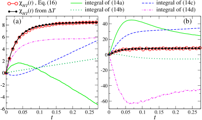
Figure 1: (Color online) Susceptibility of the internal energy to a change of $T$ in the elastic slab with fixed $T_{2}\neq T$, computed both by the direct perturbation (17) and through (16): (a) steady state at $t=0$, and (b) transient from a configuration given at $t=0$. Terms of (16) specified in (14) are also shown.

The response formula (14) simplifies when all the reservoirs are at the same temperature previous to the perturbation, because $J^{\rm{int}}=0$ and ${\mathbb{L}}^{(T)}={\mathbb{L}}$:

$$R_{{\mathcal{O}}T}(t,t^{\prime})=\sum_{i\in{\mathcal{T}}}\frac{1}{4T^{2}}\Big{\{}2{\left<{\mathcal{O}}(t)J_{i}(t^{\prime})\right>}+\frac{1}{2}\partial^{2}_{t^{\prime}}{\left<{\mathcal{O}}(t)x_{i}^{2}(t^{\prime})\right>}$$

$$\qquad+{\left<{\mathcal{O}}(t)F^{2}_{i}(t^{\prime})\right>}-{\left<{\mathcal{O}}(t)x_{i}(t^{\prime}){\mathbb{L}}F_{i}(t^{\prime})\right>}\Big{\}}.$$ (18)

Moreover, if the system is in a nonequilibrium steady state, ${\mathbb{L}}$ can be conveniently expressed in terms of the generator of the dynamics reversed in time, ${\mathbb{L}}^{*}$, as ${\mathbb{L}}={\mathbb{L}}^{*}+2\boldsymbol{v}\cdot\nabla_{\boldsymbol{x}}$, with $\boldsymbol{v}=\boldsymbol{J}/\rho$ the state velocity, i.e. the probability current over the probability density Chetrite et al. (2008). Taking for simplicity only one degree of freedom $x$, it is possible  to recast the temperature response in the form

$$R_{{\mathcal{O}}T}(t-t^{\prime})=-\frac{1}{T^{2}}\big{[}{\left<{\mathcal{O}}(t)\dot{x}(t^{\prime})F(t^{\prime})\right>}$$ (19)

$$\quad+2{\left<\partial_{x}{\mathcal{O}}(t)v(t)\dot{x}(t^{\prime})x(t^{\prime})\right>}+2{\left<{\mathcal{O}}(t)v(t^{\prime})f(t^{\prime})\right>}\big{]}.$$

In equilibrium $v=0$ and $F=-\partial_{x}{\mathcal{H}}$, hence only the entropic term $-\frac{1}{T^{2}}{\left<{\mathcal{O}}(t)\dot{x}(t^{\prime})F(t^{\prime})\right>}=\frac{1}{T^{2}}\frac{d}{dt^{\prime}}{\left<{\mathcal{O}}(t){\mathcal{H}}(t^{\prime})\right>}$ survives, and (19) correctly reduces to a Kubo formula. The nonequilibrium corrections are the correlations between the observable, the state velocity and the perturbing forces $f$ and $x$.

In conclusion, for state observables, a fluctuation-response relation to temperature changes has been derived for overdamped systems out of equilibrium, both for transient conditions and for steady states generated by nonconservative forces or by temperature gradients. The understanding of the response to temperature changes complements the previous approach based on path-weights, where the response to forces was derived Baiesi et al. (2009a, b). We can thus say that the picture of the linear response for nonequilibrium overdamped systems is almost complete. To fully close the circle, one needs the temperature response for systems with space-dependent noise prefactors, occurring for instance with hydrodynamic interactions. Investigations of these issues should consider a time rescaling, a key procedure in our approach, which leads to the concept of thermal time.

References

- Kubo (1966) R. Kubo, “The fluctuation-dissipation theorem,” Rep. Prog. Phys. 29, 255–284 (1966).
- Falcioni et al. (1990) M. Falcioni, S. Isola, and A. Vulpiani, “Correlation functions and relaxation properties in chaotic dynamics and statistical mechanics,” Phys. Lett. A 144, 341 (1990).
- Cugliandolo et al. (1994) L. Cugliandolo, J. Kurchan, and G. Parisi, “Off equilibrium dynamics and aging in unfrustrated systems,” J. Phys. I 4, 1641 (1994).
- Ruelle (1998) D. Ruelle, “General linear response formula in statistical mechanics and the fluctuation-dissipation theorem far from equilibrium,” Phys. Lett. A 245, 220–224 (1998).
- Nakamura and Sasa (2008) T. Nakamura and S.-i. Sasa, “A fluctuation-response relation of many Brownian particles under non-equilibrium conditions,” Phys. Rev. E 77, 021108 (2008).
- Chetrite et al. (2008) R. Chetrite, G. Falkovich, and K. Gawȩdzki, “Fluctuation relations in simple examples of non-equilibrium steady states,” J. Stat. Mech. , P08005 (2008).
- Speck and Seifert (2009) T. Speck and U. Seifert, “Extended fluctuation-dissipation theorem for soft matter in stationary flow,” Phys. Rev. E 79, 040102 (2009).
- Prost et al. (2009) J. Prost, J.-F. Joanny, and J. M. Parrondo, “Generalized fluctuation-dissipation theorem for steady-state systems,” Phys. Rev. Lett. 103, 090601 (2009).
- Verley et al. (2011) G. Verley, K. Mallick, and D. Lacoste, Europhys. Lett. (2011).
- Lippiello et al. (2005) E. Lippiello, F. Corberi, and M. Zannetti, “Off-equilibrium generalization of the fluctuation dissipation theorem for Ising spins and measurement of the linear response function,” Phys. Rev. E 71, 036104 (2005).
- Lippiello et al. (2007) E. Lippiello, F. Corberi, and M. Zannetti, “Fluctuation dissipation relations far from equilibrium,” J. Stat. Mech. , P07002 (2007).
- Baiesi et al. (2009a) M. Baiesi, C. Maes, and B. Wynants, “Fluctuations and response of nonequilibrium states,” Phys. Rev. Lett. 103, 010602 (2009a).
- Baiesi et al. (2009b) M. Baiesi, C. Maes, and B. Wynants, “Nonequilibrium linear response for Markov dynamics, I: Jump processes and overdamped diffusions,” J. Stat. Phys. 137, 1094–1116 (2009b).
- Chetrite (2009) R. Chetrite, “Fluctuation relations for diffusion that is thermally driven by a nonstationary bath,” Phys. Rev. E 80, 051107 (2009).
- Boksenbojm et al. (2011) E Boksenbojm, C Maes, K Netočný, and J Pešek, “Heat capacity in nonequilibrium steady states,” Europhys. Lett. 96, 40001 (2011).
- Baiesi et al. (2014) M. Baiesi, U. Basu, and C. Maes, “Thermal response in driven diffusive systems,” Eur. Phys. J. B 87, 277 (2014).
- Brandner et al. (2015) K. Brandner, K. Saito, and U. Seifert, “Thermodynamics of micro- and nano-systems driven by periodic temperature variations,” arXiv:1505.07771 (2015).
- Aguilar Sandoval et al. (2015) F. Aguilar Sandoval, M. Geitner, É. Bertin, and L. Bellon, “Resonance frequency shift of strongly heated micro-cantilevers,” J. Appl. Phys. 117, 234503 (2015).
- Conti and et al. (2012) L. Conti and et al., “Elasticity of mechanical oscillators in nonequilibrium steady states: Experimental, numerical, and theoretical results,” Phys. Rev. E 85, 066605 (2012).
- De Gregorio et al. (2011) P. De Gregorio, L. Rondoni, M. Bonaldi, and L. Conti, “One-dimensional models and thermomechanical properties of solids,” Phys. Rev. B 84, 224103 (2011).
- Lepri et al. (2003) S. Lepri, R. Livi, and A. Politi, “Thermal conduction in classical low-dimensional lattices,” Phys. Rep. 377, 1–80 (2003).
- Oono and Paniconi (1998) Y. Oono and M. Paniconi, “Steady state thermodynamics,” Progr. Theor. Phys. Suppl. 130, 29–44 (1998).
- Hatano and Sasa (2001) T. Hatano and S.-i. Sasa, “Steady-state thermodynamics of Langevin systems,” Phys. Rev. Lett. 86, 3463––3466 (2001).
- Sekimoto (2007) K Sekimoto, “Microscopic heat from the energetics of stochastic phenomena,” Phys. Rev. E 76, 060103(R) (2007).
- Sagawa and Hayakawa (2011) T. Sagawa and H. Hayakawa, “Geometrical expression of excess entropy production,” Phys. Rev. E 84, 051110 (2011).
- Bertini et al. (2013) L. Bertini, D. Gabrielli, G. Jona-Lasinio, and C. Landim, “Clausius inequality and optimality of quasistatic transformations for nonequilibrium stationary states,” Phys. Rev. Lett. 114, 020601 (2013).
- Maes and Netočný (2014) C. Maes and K. Netočný, “A nonequilibrium extension of the Clausius heat theorem,” J. Stat. Phys. 154, 188–203 (2014).
- Komatsu et al. (2015) T. S. Komatsu, N. Nakagawa, S.-i. Sasa, and H. Tasaki, “Exact equalities and thermodynamic relations for nonequilibrium steady states,” J. Stat. Phys. 159, 1237–1285 (2015).
- Mandal and Jarzynski (2015) D. Mandal and C. Jarzynski, “Analysis of slow transitions between nonequilibrium steady states,” arXiv:1507.06269 (2015).
- Abramov and Majda (2008) R. V. Abramov and A. J. Majda, “New approximations and tests of linear fluctuation-response for chaotic nonlinear forced-dissipative dynamical systems,” J. Nonlin. Sci. 18, 303–341 (2008).
- Lacorata et al. (2009) G. Lacorata, A. Puglisi, and A. Vulpiani, “On the fluctuation-response relation in geophysical systems,” Int. J. Mod. Phys. B 23, 5515–5529 (2009).
- Lucarini and Sarno (2011) V. Lucarini and S. Sarno, “A statistical mechanical approach for the computation of the climatic response to general forcings,” Nonlin. Proc. Geophys. 18, 7–28 (2011).
- Blickle et al. (2007) V. Blickle, T. Speck, U. Seifert, and C. Bechinger, “Characterizing potentials by a generalized Boltzmann factor,” Phys. Rev. E 75, 060101(R) (2007).
- Kotar et al. (2010) J. Kotar, M. Leoni, B. Bassetti, M. Cosentino Lagomarsino, and P. Cicuta, “Hydrodynamic synchronization of colloidal oscillators,” Proc. Natl. Acad. Sci. 107, 7669–7673 (2010).
- Marchetti et al. (2013) M. C. Marchetti, J. F. Joanny, S. Ramaswamy, T. B. Liverpool, J. Prost, Madan Rao, and R. Aditi Simha, “Hydrodynamics of soft active matter,” Rev. Mod. Phys. 85, 1143 (2013).
- Gomez-Solano et al. (2011) J. R. Gomez-Solano, A. Petrosyan, S. Ciliberto, and C. Maes, “Fluctuations and response in a non-equilibrium micron-sized system,” J. Stat. Mech. , P01008 (2011).
- Gomez-Solano et al. (2012) J. R. Gomez-Solano, A. Petrosyan, and S. Ciliberto, “Fluctuations, linear response and heat flux of an aging system,” Europhys. Lett. 98, 10007 (2012).
- Sekimoto (2010) K. Sekimoto, Stochastic Energetics, Lecture Notes in Physics, Vol. 799 (Springer, 2010).
- Harada and Sasa (2005) T. Harada and S.-i. Sasa, “Equality connecting energy dissipation with violation of fluctuation-response relation,” Phys. Rev. Lett. 95, 130602 (2005).
- Note (1) Note that more general conditions on and may be imposed with the same formalism.
- Riemann et al. (1996) P. Riemann, R. Bartussek, R Häussler, and P Hänggi, “Brownian motors driven by temperature oscillations,” Phys. Lett. A 215, 26–31 (1996).
- Note (2) If is a functional of the trajectory, i.e. it is extensive in time like, e.g., heat flows, the response contains the additional term .
- Zinn-Justin (2002) J. Zinn-Justin, Quantum field theory and critical phenomena, 4th ed. (Clarendon Press, Oxford, 2002).
- (44) G. Falasco, F. Baldovin, and M. Baiesi, In preparation.
- Lecomte et al. (2005) V. Lecomte, C. Appert-Rolland, and F. van Wijland, “Chaotic properties of systems with Markov dynamics,” Phys. Rev. Lett. 95, 010601 (2005).
- Merolle et al. (2005) M. Merolle, J. P. Garrahan, and D. Chandler, “Space-time thermodynampics of the glass transition,” Proc. Natl. Acad. Sci. 102, 10837–10840 (2005).
- Maes and van Wieren (2006) C. Maes and M. H. van Wieren, “Time-symmetric fluctuations in nonequilibrium systems,” Phys. Rev. Lett. 96, 240601 (2006).
- Garrahan et al. (2009) J. P. Garrahan, R. L. Jack, V. Lecomte, E. Pitard, K. van Duijvendijk, and F. van Wijland, “First-order dynamical phase transition in models of glasses: an approach based on ensembles of histories,” J. Phys. A: Math. Gen 42, 075007 (2009).
- Elmatad et al. (2010) Y. S. Elmatad, R. L. Jack, D. Chandler, and J. P. Garrahan, “Finite-temperature critical point of a glass transition,” Proc. Natl. Acad. Sci. 107, 12793–12798 (2010).
- Baiesi et al. (2010) M. Baiesi, E. Boksenbojm, C. Maes, and B. Wynants, “Linear response of nonequilibrium states, II: inertial dynamics,” J. Stat. Phys. 139, 492–505 (2010).
- Note (3) Our results can be easily generalized if a mobility (the inverse of a damping constant) is associated with each degree of freedom: one just needs the replacements and in the formulas, besides for the prefactor in the definition of the response.
- Note (4) We exploit the relations , .