Transmission problems with nonlocal boundary conditions and rough dynamic interfaces

Abstract.

We consider a transmission problem consisting of a semilinear parabolic equation in a general non-smooth setting with emphasis on rough interfaces which bear a fractal-like geometry and nonlinear dynamic (possibly, nonlocal) boundary conditions along the interface. We give a unified framework for existence of strong solutions, existence of finite dimensional attractors and blow-up phenomena for solutions under general conditions on the bulk and interfacial nonlinearities with competing behavior at infinity.

1. Introduction

In this paper we aim to give a unified framework for a general class of transmission problems of the form

$$\partial_{t}u-\text{div}\left(\mathbf{D}\nabla u\right)+f\left(u\right)=0,\;\;\;\text{ in }\;\,J\times(\Omega\backslash\Sigma),$$ (1.1)

with $J=(0,T)$, $f$ is a nonlinear function which can be either a source or a sink, and the matrix $\mathbf{D=}\left(d_{i,j}\left(x\right)\right)$ is symmetric, bounded, measurable and non-degenerate such that

$$\left\langle\mathbf{Dv,v}\right\rangle_{\mathbb{R}^{N}}\geq d_{0}\left|\mathbf{v}\right|_{\mathbb{R}^{N}}^{2},\;\mbox{ for any }\;\mathbf{v}\in{\mathbb{R}}^{N}\;\mbox{ with some constant }\;d_{0}>0.$$

In (1.1), $\Omega\subset{\mathbb{R}}^{N}$ is a bounded domain (open and connected) with Lipschitz continuous boundary $\partial\Omega$ that is disjointly decomposed into a Dirichlet part and a Neumann part, $\partial\Omega=\Gamma_{N}\cup\Gamma_{D}.$ More precisely, on $\partial\Omega$ we consider Dirichlet and Neumann boundary conditions:

$$u=0\text{ on }J\times\Gamma_{D},\text{ }(\mathbf{D}\nabla u)\cdot\nu=0\text{ on }J\times\Gamma_{N},$$ (1.2)

where $\nu$ denotes the unit outer normal vector on $\partial\Omega$. Moreover, in (1.1), $\Sigma$ is a $d$-dimensional fractal-like ”surface” contained in $\Omega\subset{\mathbb{R}}^{N}$ with $d\in(N-2,N)\cap(0,N)$. We assume that $\mathcal{H}^{d}(\Sigma)<\infty$ where $\mathcal{H}^{d}$ denotes the $d$-dimensional Hausdorff measure and we denote by $\mu_{\Sigma}$ the restriction of $\mathcal{H}^{d}$ to the set $\Sigma$. Our bounded open set $\Omega\subset\mathbb{R}^{N}$ and $\Sigma$ are such that $\Omega=\Omega_{1}\cup\Sigma\cup\Omega_{2}$ with $\Sigma=\overline{\Omega}_{1}\cap\overline{\Omega}_{2}$. That is, $\Omega$ is divided into two domains $\Omega_{1}$ and $\Omega_{2}$ with $\Omega_{1}\cap\Omega_{2}=\emptyset$ and $\Sigma$ is a $d$-dimensional surface lying strictly in $\Omega$. We notice that $\partial(\Omega\setminus\Sigma)=\partial\Omega\cup\Sigma$. We make the following convention for a function $u$ defined on $\Omega\setminus\Sigma$:

$$u(x)=u_{+}(x),\;x\in\Omega_{+}:=\Omega_{1}\;\;\mbox{ and }\;\;u(x)=u_{-}(x),\;\;x\in\Omega_{-}:=\Omega_{2}$$

and we will apply the same principle to other functions defined over $\Omega\setminus\Sigma$.

Before we give the boundary conditions that we shall consider on $\Sigma$, we have to introduce first a generalized version of a weak normal derivative of a function $u$ on the interface $\Sigma$. We notice that the definition given below is a version of the one introduced in [8, 42]. Let $\sigma$ denote the surface measure on $\partial\Omega=\Gamma_{D}\cup\Gamma_{N}$, that is, the restriction to $\partial\Omega$ of the $(N-1)$-dimensional Hausdorff measure, and recall that $\nu$ is well defined as a unit normal vector on $\partial\Omega$. Since by assumption $\Sigma$ may be so irregular that no normal vector $\nu_{\Sigma}$ can be defined on $\Sigma$, we will use the following generalized version of a normal derivative of a function on $\Sigma$. Let $\eta$ be a signed Radon measure on $\Sigma$ and $F:\overline{\Omega}\rightarrow{\mathbb{R}}^{N}$ a measurable function. If there exists a function $g\in L_{loc}^{1}({\mathbb{R}}^{N})$ satisfying

$$\int_{\Omega\backslash\Sigma}F\cdot\nabla\varphi dx=\int_{\Omega\backslash\Sigma}g\varphi dx+\int_{\partial\Omega}(F\cdot\nu)\varphi\;d\sigma+\int_{\Sigma}\varphi d\eta$$ (1.3)

for all $\varphi\in C^{1}(\overline{\Omega})$, then we say that $\eta$ is the normal measure of $F$ and we denote $N_{\Sigma}^{\star}(F):=\eta$. If the normal measure $N_{\Sigma}^{\star}(F)$ exists, then it is unique and $dN_{\Sigma}^{\star}(\psi F)=\psi dN_{\Sigma}^{\star}(F)$ for all $\psi\in C^{1}(\overline{\Omega})$. If $u\in W_{loc}^{1,1}(\Omega\backslash\Sigma)$ and $N_{\Sigma}^{\star}(\mathbf{D}\nabla u)$ exists, then we will denote by $N_{\mathbf{D}}(u):=N_{\Sigma}^{\star}(\mathbf{D}\nabla u)$ and call it the generalized $\mathbf{D}$-normal derivative of $u$ on $\Sigma$.

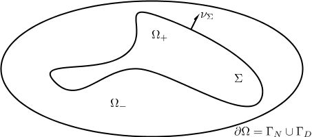
Figure 1. Example of Domain $\Omega=\Omega_{+}\cup\Sigma\cup\Omega_{-}$.

To justify this definition, assume that $\Sigma$ is a Lipschitz hypersurface of dimension $\left(N-1\right)$. Then the measure $\mu_{\Sigma}=\sigma_{\Sigma}$, the usual Lebesgue surface measure on $\Sigma$. Let $\nu_{\Sigma}$ be the exterior normal vector to $\Omega_{1}:=\Omega_{+}$ at $\Sigma$. Then the exterior normal vector to $\Omega_{2}:=\Omega_{-}$ at $\Sigma$ should be $-\nu_{\Sigma}$ (see Figure 1). Let $u\in W^{2,2}(\Omega\setminus\Sigma)$ be such that there are $g\in L_{loc}^{1}({\mathbb{R}}^{N})$ and $\tilde{g}\in L^{1}(\Sigma,\sigma_{\Sigma})$ satisfying

$$\int_{\Omega\backslash\Sigma}\mathbf{D}\nabla u\cdot\nabla\varphi dx=\int_{\Omega\backslash\Sigma}g\varphi dx+\int_{\partial\Omega}\left(\mathbf{D}\nabla u\cdot\nu\right)\varphi d\sigma+\int_{\Sigma}\tilde{g}\varphi\;d\sigma_{\Sigma}$$ (1.4)

for all $\varphi\in C^{1}(\overline{\Omega})$. On the other hand, since $u\in W^{2,2}(\Omega\setminus\Sigma)$, then using the classical Green formula (recall that we are in the situation where $\Omega\setminus\Sigma$ has a Lipschitz continuous boundary), we have that for all $\varphi\in C^{1}(\overline{\Omega})$,

$$\int_{\Omega\backslash\Sigma}\mathbf{D}\nabla u\cdot\nabla\varphi dx= -\int_{\Omega\setminus\Sigma}\mbox{div}(\mathbf{D}\nabla u)\varphi dx+\int_{\partial\Omega}\left(\mathbf{D}\nabla u\cdot\nu\right)\varphi d\sigma$$ (1.5)

$$+\int_{\Sigma}\varphi\left(\mathbf{D}_{+}\nabla u_{+}-\mathbf{D}_{-}\nabla u_{-}\right)\cdot\nu_{\Sigma}d\sigma_{\Sigma}.$$

Moreover, $\mbox{div}(\mathbf{D}\nabla u)\in L^{2}(\Omega\setminus\Sigma)$, $\left(\mathbf{D}\nabla u\cdot\nu\right)\in L^{2}(\partial\Omega)$ and $\left(\mathbf{D}_{+}\nabla u_{+}-\mathbf{D}_{-}\nabla u_{-}\right)\cdot\nu_{\Sigma}\in L^{2}(\Sigma)$. It follows from (1.4) and (1.5) that in this case, $g=-\mbox{div}(\mathbf{D}\nabla u)$ and $\tilde{g}=\left(\mathbf{D}\nabla u_{+}-\mathbf{D}\nabla u_{-}\right)\cdot\nu_{\Sigma}$ so that

$$dN_{\mathbf{D}}(u):=dN_{\Sigma}^{\star}(\mathbf{D}\nabla u)=\tilde{g}d\sigma_{\Sigma}=\left(\left(\mathbf{D}_{+}\nabla u_{+}-\mathbf{D}_{-}\nabla u_{-}\right)\cdot\nu_{\Sigma}\right)d\sigma_{\Sigma}\;\;\mbox{ on }\;\Sigma,$$

and hence,

$$\frac{dN_{\mathbf{D}}(u)}{d\sigma_{\Sigma}}=\left(\mathbf{D}_{+}\nabla u_{+}-\mathbf{D}_{-}\nabla u_{-}\right)\cdot\nu_{\Sigma}\;\;\mbox{ on }\;\Sigma.$$

We will always use the generalized Green type identity (1.3) and the generalized $\mathbf{D}$-normal derivative of a function $u$ on $\Sigma$ introduced above.

Now, on the interfacial region $\Sigma$ we impose the dynamic boundary condition formally given by

$$dN_{\mathbf{D}}(u)+\left(\delta\partial_{t}u+\beta\left(x\right)u+\Theta_{{\Sigma}}\left(u\right)\right)d\mu_{\Sigma}=h\left(u\right)d\mu_{\Sigma},\;\;\text{ on }\;\,J\times\Sigma,$$ (1.6)

where we are primarily interested in nonlinear sources at the interface $\Sigma$ such that

$$\underset{\left|\tau\right|\rightarrow\infty}{\lim\inf}\frac{h\left(\tau\right)}{\tau}=\infty.$$ (1.7)

The function $\beta\in L^{\infty}(\Sigma,\mu_{\Sigma})$ satisfies $\beta(x)\geq 0$ for $\mu_{\Sigma}$-a.e. $x\in\Sigma$ but it is not identically equal to zero on $\Sigma$ and $\delta\geq 0$ is a real number. Note that the condition on $h$ implies that $h$ has a bad sign and is of superlinear growth at infinity (i.e., $h\left(\tau\right)\sim c_{h}\left|\tau\right|^{\alpha}\tau,$ as $\left|\tau\right|\rightarrow\infty$, for some $\alpha>0$ and $c_{h}>0$). In (1.6), we define $\Theta_{{\Sigma}}$ as a non-local operator in the following fashion (see Section 2.2 below):

$$\langle\Theta_{{\Sigma}}(u),v\rangle:=\int\int_{\Sigma\times\Sigma}K(x,y)(u(x)-u(y))(v(x)-v(y))d\mu_{\Sigma}\left(x\right)d\mu_{\Sigma}\left(y\right),$$ (1.8)

for functions $u,v\in\widetilde{W}^{1,2}(\Omega)$ such that $\Theta_{\Sigma}(u)\in L^{2}(\Sigma,d\mu_{\Sigma})$ and

$$\int\int_{\Sigma\times\Sigma}K(x,y)|u(x)-u(y)|^{2}d\mu_{\Sigma}(x)d\mu_{\Sigma}(y),\;\;\int\int_{\Sigma\times\Sigma}K(x,y)|v(x)-v(y)|^{2}d\mu_{\Sigma}(x)d\mu_{\Sigma}(y)<\infty,$$

where the kernel $K:\Sigma\times\Sigma\rightarrow\mathbb{R}_{+}$ is symmetric and satisfies

$$c_{0}\leq K\left(x,y\right)\left|x-y\right|^{d+2s}\leq c_{1},$$

for all $x,y\in\Sigma$, $x\neq y$, for some constants $c_{0},c_{1}>0$ and $s\in\left(0,1\right)$. A basic example is $K\left(x,y\right)=\left|x-y\right|^{-\left(d+2s\right)}$. In this case, $\Theta_{\Sigma}=\left(-\Delta_{\Sigma}\right)^{s}$ is a nonlocal operator characterizing the presence of anomalous ”fractional” diffusion along $\Sigma$. The $\mathbf{D}$-normal derivative $N_{\mathbf{D}}(u)$ of $u$ in (1.6) is understood in the sense of (1.3). We mention that if $\Sigma$ is a Lipschitz hypersurface of dimension $(N-1)$, then the condition (1.6) reads

$$\left(\mathbf{D}_{+}\nabla u_{+}-\mathbf{D}_{-}\nabla u_{-}\right)\cdot\nu_{\Sigma}+\left(\delta\partial_{t}u+\beta\left(x\right)u+\Theta_{{\Sigma}}\left(u\right)\right)=h\left(u\right),\;\;\text{ on }\,\;J\times\Sigma.$$

Finally, initial conditions for (1.1), (1.2) and (1.6) must also be prescribed on $\Omega\backslash\Sigma$ and on $\Sigma,$ respectively.

The interface problem (1.1), (1.2) and (1.6) with a more simple transmission condition (1.6) on $\Sigma$, i.e. when $\delta=0,$ $\Theta_{{\Sigma}}\equiv 0$ and $h\equiv 0$, is often encountered in the literature in heat transfer phenomena, fluid dynamics and material science, and in electrostatics and magnetostatics. It is the usual case when two bodies materials or fluids with different conductivities or diffusions are involved. The corresponding transmission problem for the linear elliptic equation assuming that the interface $\Sigma$ is at least Lipschitz smooth and $\Theta_{{\Sigma}}\equiv 0$, $h\equiv 0$, has been considered by a large group of mathematicians including O.A. Ladyzhenskaya and N.N. Ural’tseva since the 1970’s (see [18, 27]). We also refer the reader to the recent book of Borsuk [9]. Under the same foregoing assumptions the (linear) parabolic transmission problem has also been investigated recently in [4, 25, 27, 30, 37] (and the references therein) in the case when $\delta=0$ and $\Theta_{{\Sigma}}\equiv 0,h\equiv 0$. The transmission problem (1.1) with a linear dynamic (i.e., when $\delta>0$) transmission condition on a smooth surface $\Sigma$ (so it can be flattened) and its influence of the solution was studied in [5] in the autonomous case. Finally, a linear interface problem with linear dynamic transmission condition involving the surface diffusion $\Delta_{\Sigma}$ on $\Sigma$ and allowing both cases in which $\mathbf{D}$ is nondegenerate and degenerate, and when the interface $\Sigma$ is a $\left(N-1\right)$-dimensional Lipschitz hypersurface was also considered in [15, 17]. When $\Sigma$ is rough and fractal-like has also attracted considerable interest over the recent years due to their importance in various engineering, physical and natural processes, such as, “hydraulic fracturing”, a frequently used engineering method to increase the flow of oil from a reservoir into a producing oil well [10, 28], current flow through rough electrodes in electrochemistry [11, 19, 40] or diffusion and biological processes across irregular physiological membranes [31, 32, 33, 34].

It is our goal to give a unified analysis of these transmission problems for a large class of fractal-like interfaces, to go beyond the present studies which have focused mainly on the linear interface problem with linear transmission conditions and mainly well-posedness like results. We will derive stronger and sharper results in terms of existence, regularity and stability of bounded solutions. Then we also show the existence of finite dimensional attractors for the nonlinear transmission problem (1.1), (1.2) and (1.6) especially in non-dissipative situations in which a bad source $h$ (via (1.7)) is present along $\Sigma$ such that energy is always fed in all of $\Omega\backslash\Sigma$ through $\Sigma$ but eventually dissipated completely by a nonlinear ”good” source $f$. It turns out that blow-up phenomena and global existence are strictly related to competing conditions and the behavior of the nonlinearities $f,h$ at infinity as $\left|\tau\right|\rightarrow\infty$. We state sharp balance conditions between the bulk source/sink $f$ and interfacial source $h$ allowing us to directly compare them even when they are acting on separate parts of the domain $\Omega,$ on $\Omega\backslash\Sigma$ and on $\Sigma$, respectively. Notably, similar ideas have been used by Gal [21] in the treatment of parabolic $p$-Laplace equations with nonlinear reactive-like dynamic boundary conditions (cf. also Bernal and Tajdine [38] for parabolic problems subject to nonlinear Robin conditions), and by Gal and Warma in [23] to give a complete characterization of the long-time behavior as time goes to infinity (in terms of a finite dimensional global attractor, $\omega$-limit sets and Lyapunov functions) for semilinear parabolic equations on rough domains subject to nonlocal Robin boundary conditions. Since most of the aforementioned applications have a real physical meaning in non-reflexive Banach spaces, like $L^{1}\left(\Omega\right)$ or $L^{\infty}\left(\Omega\right)$, our prefered notion of generalized solutions and nonlinear solution semigroups will naturally be given in $L^{\infty}$-type spaces. It is this context in which in fact our balance conditions on the nonlinearities become also optimal and sharp in a certain sense. In this work, we also develop a unified framework in order to resolve the difficulties coming from having to deal with a rough fractal-like interface $\Sigma$, and develop new tools based on potential analysis to handle the present case. This new approach allows us to not only overcome the difficulties mentioned earlier, but also to do so using only elementary tools from Sobolev spaces, nonlinear semigroup theory and dynamical systems theory avoiding the use of sophisticated tools from harmonic analysis.

The remainder of the paper is structured as follows. In Section 2, we establish our notation and give some basic preliminary results for the operators and spaces appearing in our transmission model. In Section 3, we prove some well-posedness results for this model; in particular, we establish existence and stability results for strong solutions. In Section 4, we prove results which establish the existence of global and exponential attractors for (1.1), (1.2) and (1.6). Section 5 contains some new results on the blow-up of strong solutions.

2. Some generation of semigroup results

In this section we introduce the functional framework associated with the transmission problem in question and then derive semigroup type results for the linear operator corresponding to the linear problem. All these tools are necessary in the study of the nonlinear transmission problem (1.1), (1.2) and (1.6).

2.1. Functional framework

Let $\Omega\subset{\mathbb{R}}^{N}$ be a bounded open set with boundary $\partial\Omega$ and $1\leq p<\infty$. We denote by

$$W^{1,p}(\Omega):=\{u\in L^{p}(\Omega):\;\int_{\Omega}|\nabla u|^{p}dx<\infty\}$$

the first order Sobolev space endowed with the norm

$$\|u\|_{W^{1,p}(\Omega)}:=\left(\int_{\Omega}|u|^{p}\;dx+\int_{\Omega}|\nabla u|^{p}dx\right)^{\frac{1}{p}}.$$

We let

$$\widetilde{W}^{1,p}(\Omega):=\overline{W^{1,p}(\Omega)\cap C(\overline{\Omega})}^{W^{1,p}(\Omega)}\;\;\mbox{ and }\;W_{0}^{1,p}(\Omega):=\overline{\mathcal{D}(\Omega)}^{W^{1,p}(\Omega)},$$

where $\mathcal{D}(\Omega)$ denotes the space of test functions on $\Omega$. It is well-known that $\widetilde{W}^{1,p}(\Omega)$ is a proper closed subspace of $W^{1,p}(\Omega)$ but the two spaces coincide if $\Omega$ has a continuous boundary (see., e.g. [36, Theorem 1 p.23]). Moreover, by definition, $W_{0}^{1,p}(\Omega)$ is a closed subspace of $\widetilde{W}^{1,p}(\Omega)$ and hence, of $W^{1,p}(\Omega)$. Next, let $\Gamma\subset\partial\Omega$ be a closed set. We denote by $W_{0,\Gamma}^{1,p}(\Omega)$ the closure of the set

$$\{u\in W^{1,p}(\Omega)\cap C(\overline{\Omega}):\;u=0\;\mbox{ on }\;\Gamma\}\;\;\text{ in }\;\;W^{1,p}(\Omega)$$

so that $W_{0}^{1,p}(\Omega)$ coincides with $W_{0,\partial\Omega}^{1,p}(\Omega)$.

Definition 2.1.

Let $p\in[1,\infty)$ be fixed. We will say that a given open set $\Omega\subset{\mathbb{R}}^{N}$ has the ${W}^{1,p}$-extension property, if for every $u\in{W}^{1,p}(\Omega)$, there exists $U\in W^{1,p}({\mathbb{R}}^{N})$ such that $U|_{\Omega}=u$. Similarly, we will say that $\Omega$ has the $\widetilde{W}^{1,p}$-extension property, if for every $u\in\widetilde{W}^{1,p}(\Omega)$, there exists $U\in W^{1,p}({\mathbb{R}}^{N})$ such that $U|_{\Omega}=u$. In that case, the extension operator $E:\;W^{1,p}(\Omega)\rightarrow W^{1,p}({\mathbb{R}}^{N})$ (resp., $\widetilde{E}:\;\widetilde{W}^{1,p}(\Omega)\rightarrow W^{1,p}({\mathbb{R}}^{N})$ is linear and bounded, that is, there exists a constant $C>0$ such that for every $u\in W^{1,p}(\Omega)$ (resp., $u\in\widetilde{W}^{1,p}(\Omega)$),

$$\|Eu\|_{W^{1,p}({\mathbb{R}}^{N})}=\|U\|_{W^{1,p}({\mathbb{R}}^{N})}\leq C\|u\|_{W^{1,p}(\Omega)}.$$

(resp., $\|\widetilde{E}u\|_{W^{1,p}({\mathbb{R}}^{N})}=\|U\|_{W^{1,p}({\mathbb{R}}^{N})}\leq C\|u\|_{W^{1,p}(\Omega)}$). See [26] for further details.

If $\Omega$ has the $W^{1,p}$-extension property, then there exists a constant $C>0$ such that for every $u\in W^{1,p}(\Omega)$,

$$\|u\|_{L^{q}(\Omega)}\leq C\|u\|_{W^{1,p}(\Omega)},\;\;q\in[1,p^{\star}],\;p^{\star}:=\frac{Np}{N-p},\;\mbox{ if }\;N>p,\;\;q\in[1,\infty)\;\mbox{ if }\;N=p.$$ (2.1)

Moreover,

$$W^{1,p}(\Omega)\hookrightarrow C^{0,1-\frac{N}{p}}(\overline{\Omega})\;\;\mbox{ if }\;N<p.$$ (2.2)

The embedding (2.1) and (2.2) remain valid with $W^{1,p}(\Omega)$ replaced by $\widetilde{W}^{1,p}(\Omega)$, if $\Omega$ is assumed to have the $\widetilde{W}^{1,p}$-extension property. In particular, all these statements are true if $\Omega$ has a Lipschitz continuous boundary $\partial\Omega.$

Remark 2.2.

We mention that if $\Omega$ has the $W^{1,p}$-extension property, then $\widetilde{W}^{1,p}(\Omega)=W^{1,p}(\Omega)$ and hence, $\Omega$ has the $\widetilde{W}^{1,p}$-extension property. For instance, in two dimensions the open set $\Omega:=B(0,1)\backslash[-1,1]\times\{0\}\subset\mathbb{R}^{2}$ enjoys the $\widetilde{W}^{1,p}$-extension property for any $p\in[1,\infty)$ but does not possess the $W^{1,p}$-extension property (see e.g. [7]). In general if $p\in(1,\infty)$ and $\Omega\subset{\mathbb{R}}^{N}$ has the $W^{1,p}$-extension property and $F\subset\Omega$ is a relatively closed set with $\mathcal{H}^{N-1}(F)<\infty$ (i.e., the $(N-1)$-dimensional Hausdorff measure $\mathcal{H}^{N-1}$ of $F$ is finite), then the open set $\Omega\backslash F$ has the $\widetilde{W}^{1,p}$-extension property. However, generally it may happen (as the case of the two dimensional example given above) that $\Omega\backslash F$ does not possess the $W^{1,p}$-extension property (see e.g. [7] for other examples and for more details on this subject).

Definition 2.3.

Let $F\subset{\mathbb{R}}^{N}$ be a compact set, $d\in(0,N]$ and $\mu$ a regular Borel measure on $F$. We say that $\mu$ is an upper $d$-Ahlfors measure if there exists a constant $C>0$ such that for every $x\in F$ and every $r\in(0,1]$, one has

$$\mu(B(x,r)\cap F)\leq Cr^{d}.$$

Remark 2.4.

Let $\Omega\subset\mathbb{R}^{N}$ be an arbitrary bounded domain with boundary $\partial\Omega$. Let $1<p<\infty$ and $d\in(N-p,N)\cap(0,N)$ be the Hausdorff dimension of $\partial\Omega$. Assume also that $\Omega$ has the $W^{1,p}$-extension property. Then $\mathcal{H}_{\mid\partial\Omega}^{d}$ is an upper $d$-Ahlfors measure. For instance, if $\Omega\subset\mathbb{R}^{2}$ is the bounded domain enclosed by the Koch curve, then $\mathcal{H}_{\mid\partial\Omega}^{d}\left(\partial\Omega\right)<\infty$ where $d=\ln(4)/\ln(3)$ is the Hausdorff dimension of $\partial\Omega$. Moreover $\Omega$ has the $W^{1,p}$-extension property and the restriction of $\mathcal{H}^{d}$ to $\partial\Omega$ is an upper $d$-Ahlfors measure (see [6, 24, 29]).

Next, let $S\subset{\mathbb{R}}^{N}$ be a compact set, $\mu$ an upper $d$-Ahlfors measure on $S$ for some $d\in(N-2,N)\cap(0,N)$ and let $0<s<1$. We define the fractional order Sobolev space

$$\mathbb{B}_{d,s}^{2}(S,\mu):=\{u\in L^{2}(S,\mu):\;\int_{S}\int_{S}\frac{|u(x)-u(y)|^{2}}{|x-y|^{d+2s}}d\mu(x)d\mu(y)<\infty\}$$

and we endow it with the norm

$$\|u\|_{\mathbb{B}_{d,s}^{2}(S,\mu)}:=\left(\int_{S}|u|^{2}d\mu+\int_{S}\int_{S}\frac{|u(x)-u(y)|^{2}}{|x-y|^{d+2s}}d\mu(x)d\mu(y)\right)^{\frac{1}{2}}.$$

The following result is taken from [6, Theorems 1.1 and 6.7] (see also [13]).

Theorem 2.5.

Let $\Omega\subset{\mathbb{R}}^{N}$ be a bounded open set and assume that it has the $W^{1,2}$-extension property. Let $S\subset\overline{\Omega}$ be a compact set and $\mu$ an upper $d$-Ahlfors measure on $S$ for some $d\in(N-2,N)\cap(0,N)$. Then the following assertions hold.

1. There exists a constant $C>0$ such that for every $u\in W^{1,2}(\Omega)$,

   $$\|u\|_{L^{2_{\star}}(S,\mu)}\leq C\|u\|_{W^{1,2}(\Omega)},\;\;2_{\star}:=\frac{2d}{N-2}>2.$$ (2.3)

2. For every $0<s<1-\frac{N-d}{2}$, there exists a constant $C>0$ such that for every $u\in W^{1,2}(\Omega)$,

   $$\|u\|_{\mathbb{B}_{d,s}^{2}(S,\mu)}\leq C\|u\|_{W^{1,2}(\Omega)}.$$ (2.4)

We notice that the estimates (2.3) and (2.4) remain valid with $W^{1,2}(\Omega)$ replaced by $\widetilde{W}^{1,2}(\Omega)$ if $\Omega$ is assumed to have the $\widetilde{W}^{1,2}$-extension property.

Next, we introduce the notion of Dirichlet form on an $L^{2}$-type space (see [20, Chapter 1]). To this end, let $X$ be a locally compact metric space and $\eta$ a Radon measure on $X$. Let $L^{2}(X,\eta)$ be the real Hilbert space with inner product $\left(\cdot,\cdot\right)$ and let $\mathcal{E}$ with domain $D(\mathcal{E})$ be a bilinear form on $L^{2}(X,\eta)$.

Definition 2.6.

The form $\mathcal{E}$ is said to be a Dirichlet form if the following conditions hold:

1. $\mathcal{E}:D\left(\mathcal{E}\right)\times D\left(\mathcal{E}\right)\rightarrow\mathbb{R}$, where the domain $D\left(\mathcal{E}\right)$ of the form is a dense linear subspace of $L^{2}(X,\eta).$

2. $\mathcal{E}\left(u,v\right)=\mathcal{E}\left(v,u\right)$, $\mathcal{E}\left(u+v,w\right)=\mathcal{E}\left(u,w\right)+\mathcal{E}\left(v,w\right)$, $\mathcal{E}\left(au,v\right)=a\mathcal{E}\left(u,v\right)$ and $\mathcal{E}\left(u,u\right)\geq 0$, for all $u,v,w\in D\left(\mathcal{E}\right)$ and $a\in\mathbb{R}$.

3. Let $\lambda>0$ and define $\mathcal{E}_{\lambda}\left(u,v\right)=\mathcal{E}\left(u,v\right)\mathcal{+\lambda}\left(u,v\right),$ for $u,v\in D\left(\mathcal{E}_{\lambda}\right)=D\left(\mathcal{E}\right)$. The form $\mathcal{E}$ is closed, that is, if $u_{n}\in D\left(\mathcal{E}\right)$ with $\mathcal{E}_{\lambda}\left(u_{n}-u_{m},u_{n}-u_{m}\right)\rightarrow 0$ as $n,m\rightarrow\infty$, then there exists $u\in D\left(\mathcal{E}\right)$ such that $\mathcal{E}_{\lambda}\left(u_{n}-u,u_{n}-u\right)\rightarrow 0$ as $n\rightarrow\infty.$

4. For each $\epsilon>0$ there exists a function $\phi_{\epsilon}:\mathbb{R}\rightarrow\mathbb{R}$, such that $\phi_{\epsilon}\in C^{\infty}({\mathbb{R}})$, $\phi_{\epsilon}\left(t\right)=t,$ for $t\in\left[0,1\right],$ $-\epsilon\leq\phi_{\epsilon}\left(t\right)\leq 1+\epsilon$, for all $t\in\mathbb{R}$, $0\leq\phi_{\epsilon}\left(t\right)-\phi_{\epsilon}\left(\tau\right)\leq t-\tau$, whenever $\tau<t$, such that $u\in D\left(\mathcal{E}\right)$ implies $\phi_{\epsilon}\left(u\right)\in D\left(\mathcal{E}\right)$ and $\mathcal{E}\left(\phi_{\epsilon}\left(u\right),\phi_{\epsilon}\left(u\right)\right)\leq\mathcal{E}\left(u,u\right).$

Remark 2.7.

Clearly, $D\left(\mathcal{E}\right)$ is a real Hilbert space with inner product $\mathcal{E}_{\lambda}\left(u,u\right)$ for each $\lambda>0$. We recall that a form $\mathcal{E}$ which satisfies (a)-(c) is closed and symmetric. If $\mathcal{E}$ also satisfies (d), then it is said to be a Markovian form.

Let $T=(T(t))_{t\geq 0}$ be a semigroup on $L^{2}(X,\eta)$. We say that $T(t)$ is positively-preserving, if $T(t)u\geq 0$ $\eta$-a.e. and for all $t\geq 0$, whenever $u\in L^{2}(X,\eta)$ and $u\geq 0$ $\eta$-a.e. If $T(t)$ is positively-preserving and $T(t)$ is a contraction on $L^{\infty}(X,\eta)$, that is,

$$\|T(t)u\|_{L^{\infty}(X,\eta)}\leq\|u\|_{L^{\infty}(X,\eta)},\;\forall\;t\geq 0,\;\forall\;u\in L^{2}(X,\eta)\cap L^{\infty}(X,\eta),$$

then we will say that $T=(T(t))_{t\geq 0}$ is a Markovian (or submarkovian) semigroup. It turns out that if $A$ is the closed linear self-adjoint operator in $L^{2}(X,\mu)$ associated with the Dirichlet form $\mathcal{E}$, then $-A$ generates a strongly continuous Markovian semigroup on $L^{2}(X,\eta)$. Conversely, the generator of every symmetric, strongly continuous Markovain semigroup on $L^{2}(X,\eta)$ is given by a Dirichlet form on $L^{2}(X,\eta)$. For more details on this topic we refer to Chapter 1 of the monographs [14, 20].

2.2. The non-local dynamic boundary conditions on the interface

Throughout the remainder of the article the sets $\Omega$, $\partial\Omega$, $\Gamma_{N}$, $\Gamma_{D}$ and $\Sigma$ are as defined in the introduction. Recall that $\Sigma\subset\Omega$ is a relatively closed set with Hausdorff dimension $d\in(N-2,N)\cap(0,N)$ and that $\mathcal{H}^{d}(\Sigma)<\infty$ where $\mathcal{H}^{d}$ denotes the $d$-dimensional Hausdorff measure. We still denote by $\mu_{\Sigma}$ the restriction of $\mathcal{H}^{d}$ to the set $\Sigma$. In this case, we have that $\mu_{\Sigma}$ is an upper $d$-Ahlfors measure on $\Sigma$ (see e.g. [7, 29]). Recall also that

$$\widetilde{W}^{1,2}(\Omega\backslash\Sigma):=\overline{W^{1,2}(\Omega\backslash\Sigma)\cap C(\overline{\Omega})}^{W^{1,2}(\Omega\backslash\Sigma)}.$$

Remark 2.8.

In general, even if $\mathcal{H}^{N}(\Sigma)=0$, the space $\widetilde{W}^{1,2}(\Omega\backslash\Sigma)$ is not equal to $\widetilde{W}^{1,2}(\Omega)=W^{1,2}(\Omega)$. But if $d=N-1$, then it follows from [7, Proposition 3.6] that

$$W^{1,2}(\Omega)=\widetilde{W}^{1,2}(\Omega)=\widetilde{W}^{1,2}(\Omega\backslash\Sigma).$$

Let

$${W}_{0,\Gamma_{D}}^{1,2}(\Omega\backslash\Sigma)=\overline{\{u\in{W}^{1,2}(\Omega\backslash\Sigma)\cap C(\overline{\Omega}):\;u=0\;\mbox{ on }\Gamma_{D}\}}^{{W}^{1,2}(\Omega\backslash\Sigma)}.$$

By definition, we have that ${W}_{0,\Gamma_{D}}^{1,2}(\Omega\backslash\Sigma)$ is a closed subspace of $\widetilde{W}^{1,2}(\Omega\backslash\Sigma)$.

For $r,q\in[1,\infty]$ with $1\leq r,q<\infty$ or $r=q=\infty$ we endow the Banach space

$$\mathbb{X}^{r,q}(\Omega,\Sigma):=L^{r}(\Omega)\times L^{q}(\Sigma,\mu_{\Sigma})=\{(f,g),\;f\in L^{r}(\Omega),\;g\in L^{q}(\Sigma,\mu_{\Sigma})\}$$

with the norm

$$\|(f,g)\|_{\mathbb{X}^{r,q}(\Omega,\Sigma)}:=\|f\|_{r,\Omega}+\|g\|_{q,\Sigma}\;\mbox{ if }\;r\neq q,\;\|(f,g)\|_{\mathbb{X}^{r,r}(\Omega,\Sigma)}:=(\|f\|_{r,\Omega}^{r}+\|g\|_{r,\Sigma}^{r})^{\frac{1}{r}}$$

if $1\leq r,q<\infty$ and

$$\|(f,g)\|_{\mathbb{X}^{\infty,\infty}(\Omega,\Sigma)}:=\max\{\|f\|_{\infty,\Omega},\|g\|_{\infty,\Sigma}\}.$$

We will simple write $\mathbb{X}^{r}(\Omega,\Sigma):=\mathbb{X}^{r,r}(\Omega,\Sigma)$. If $\Omega\backslash\Sigma$ has the $\widetilde{W}^{1,2}$-extension property, then identifying each function $u\in\widetilde{W}^{1,2}(\Omega\backslash\Sigma)$ with $(u,u|_{\Sigma})$ (recall that in this case, by Theorem 2.5, every $u\in\widetilde{W}^{1,2}(\Omega\backslash\Sigma)$ has a well-defined trace $u|_{\Sigma}$ which belongs to some $L^{q}(\Sigma,\mu_{\Sigma})$), we get from (2.1) and (2.3) that if $N>2$, then

$$\widetilde{W}^{1,2}(\Omega\backslash\Sigma)\hookrightarrow\mathbb{X}^{r,q}(\Omega,\Sigma),\;\;\forall\;r\in[1,2^{\star}],\;2^{\star}:=\frac{2N}{N-2},\;\forall\;q\in[1,2_{\star}],\;\;2_{\star}:=\frac{2d}{N-2}.$$ (2.5)

Remark 2.9.

Recall that by definition, $W_{0,\Gamma_{D}}^{1,2}(\Omega\backslash\Sigma)$ is a closed subspace of $\widetilde{W}^{1,2}(\Omega\backslash\Sigma)$. Let $Cap$_Ω∖Σ be the relative capacity defined with on subsets of $\overline{\Omega\setminus\Sigma}=\overline{\Omega}$, with the regular (in these sense of [20, p.6]) Dirichlet space $\widetilde{W}^{1,2}(\Omega\backslash\Sigma)$. More precisely, for a subset $A$ of $\overline{\Omega}$, let

$$Cap_{{}_{\Omega\setminus\Sigma}}\left(A\right):=\inf\left\{\|u\|_{\widetilde{W}^{1,2}(\Omega\backslash\Sigma)}^{2}\;:\;\begin{array}[]{l}u\in\widetilde{W}^{1,2}(\Omega\backslash\Sigma),\;\exists\;O\subset{\mathbb{R}}^{N}\text{ open,}\\ A\subset O\text{ and }u\geq 1\text{ a.e. on }\overline{\Omega\setminus\Sigma}\cap O\end{array}\right\}.$$

With respect to the capacity $Cap$_Ω∖Σ, every function $u\in W_{0,\Gamma_{D}}^{1,2}(\Omega\backslash\Sigma)$ has a unique (relatively quasi-everywhere) relatively quasi-continuous version $\tilde{u}$ on $\overline{\Omega}$. Throughout the rest of the paper, if $u\in W_{0,\Gamma_{D}}^{1,2}(\Omega\backslash\Sigma)$, by $u|_{\Sigma}$, we mean $\tilde{u}|_{\Sigma}$. If $\Omega\backslash\Sigma$ has the $\widetilde{W}^{1,2}$-extension property then $u|_{\Sigma}=\tilde{u}|_{\Sigma}$ coincides with the trace of $u$ on $\Sigma,$ which exists by Theorem 2.5 and belongs to $L^{2_{\star}}(\Sigma,\mu_{\Sigma})$.

Next, let $0<s<1$ and define the bilinear symmetric form ${\mathcal{A}}_{\Theta,{\Sigma}}$ on $\mathbb{X}^{2}(\Omega,\Sigma)$ with domain

$$D({\mathcal{A}}_{\Theta,{\Sigma}})=\{U:=(u,u|_{\Sigma}),\;u\in W_{0,\Gamma_{D}}^{1,2}(\Omega\backslash\Sigma),\;u|_{\Sigma}\in\mathbb{B}_{d,s}^{2}(\Sigma,\mu_{\Sigma})\}$$ (2.6)

and given for $U:=(u,u|_{\Sigma}),\Phi:=(\varphi,\varphi|_{\Sigma})\in D({\mathcal{A}}_{\Theta,{\Sigma}})$ by

$${\mathcal{A}}_{\Theta,{\Sigma}}(U,\Phi)= \int_{\Omega\backslash\Sigma}\mathbf{D}\nabla u\cdot\nabla\varphi dx+\int_{\Sigma}\beta\left(x\right)u\varphi d\mu_{\Sigma}$$ (2.7)

$$+\int_{\Sigma}\int_{\Sigma}K(x,y)(u(x)-u(y))(\varphi(x)-\varphi(y))d\mu_{\Sigma}\left(x\right)d\mu_{\Sigma}\left(y\right),$$

where we recall $\mathbf{D}=(d_{ij}(x))$ is symmetric, bounded, measurable and non-degenerate such that

$$\left\langle\mathbf{Dv,v}\right\rangle_{\mathbb{R}^{N}}\geq d_{0}\left|\mathbf{v}\right|_{\mathbb{R}^{N}}^{2},\;\mbox{ for any }\;\mathbf{v}\in{\mathbb{R}}^{N}\;\mbox{ with some constant }\;d_{0}>0,$$ (2.8)

and the symmetric kernel $K$ is such that there exist two constants $0<c_{0}\leq c_{1}$ satisfying

$$c_{0}\leq K(x,y)|x-y|^{d+2s}\leq c_{1},\;\;\forall\;x,y\in\Sigma,\;x\neq y.$$

The function $\beta\in L^{\infty}(\Sigma,\mu_{\Sigma})$ and there exists a constant $\beta_{0}$ such that

$$\beta(x)\geq\beta_{0}>0\;\mbox{ for }\;\mu_{\Sigma}-\mbox{a.e. }\;x\in\Sigma.$$ (2.9)

We notice that $D({\mathcal{A}}_{\Theta,{\Sigma}})$ is not empty, since it contains the set $\{(u,u|_{\Sigma}):\;u\in C^{1}(\overline{\Omega}):\;u=0\;\mbox{ on }\;\Gamma_{D}\}$ and in particular it contains $\{(u,u|_{\Sigma})=(u,0):\;u\in\mathcal{D}(\Omega\setminus\Sigma)\}$.

Remark 2.10.

We mention that if $0<s<1-\frac{N-d}{2}$ and $\Omega\backslash\Sigma$ has the $\widetilde{W}^{1,2}$-extension property, then it follows from Theorem 2.5-(b) that

$$D(\mathcal{A}_{\Theta,{\Sigma}})=\{U=(u,u|_{\Sigma}):\;u\in W_{0,\Gamma_{D}}^{1,2}(\Omega\backslash\Sigma)\}.$$

Throughout this section, in order to apply the abstract result on Dirichlet forms given in Definition 2.6, we notice that $\mathbb{X}^{2}(\Omega,\Sigma)$ can be identified with $L^{2}(\Omega,\eta)$ where the measure $\eta:=\mathcal{H}^{N}\oplus\mu_{\Sigma}$ is given for every measurable set $B\subset\Omega$ by $\eta(B)=\mathcal{H}^{N}(B\cap(\Omega\setminus\Sigma))+\mu_{\Sigma}(B\cap\Sigma)$, so that for every $u\in L^{2}(\Omega,\eta)$, we have

$$\int_{\Omega}ud\eta=\int_{\Omega\setminus\Sigma}udx+\int_{\Sigma}ud\mu_{\Sigma}.$$

We have the following result.

Proposition 2.11.

Assume that $\Sigma$ is such that $\mu_{\Sigma}$ is absolutely continuous with respect to $Cap_{\Omega\setminus\Sigma}$, that is,

$$Cap_{\Omega\setminus\Sigma}(B)=0\;\Longrightarrow\;\mu_{\Sigma}(B)=0\;\mbox{ for all Borel set }\;B\subset\Sigma.$$ (2.10)

The bilinear symmetric form ${\mathcal{A}}_{\Theta,{\Sigma}}$ with domain $D({\mathcal{A}}_{\Theta,{\Sigma}})$ is a Dirichlet form in the space $\mathbb{X}^{2}(\Omega,\Sigma)$, that is, it is closed and Markovian.

Proof.

Let ${\mathcal{A}}_{\Theta,{\Sigma}}$ with domain $D({\mathcal{A}}_{\Theta,{\Sigma}})$ be the bilinear symmetric form in $\mathbb{X}^{2}(\Omega,\Sigma)$ defined in (2.7). First we show that the form ${\mathcal{A}}_{\Theta,{\Sigma}}$ is closed in $\mathbb{X}^{2}(\Omega,\Sigma)$. Indeed, let $U_{n}=(u_{n},u_{n}|_{\Sigma})\in D(\mathcal{A}_{\Theta,{\Sigma}})$ be a sequence such that

$$\lim_{n,m\rightarrow\infty}\left(\mathcal{A}_{\Theta,{\Sigma}}(U_{n}-U_{m},U_{n}-U_{m})+\|u_{n}-u_{m}\|_{L^{2}(\Omega)}^{2}+\|u_{n}-u_{m}\|_{L^{2}(\Sigma,\mu_{\Sigma})}^{2}\right)=0.$$ (2.11)

It follows from (2.11) that $\lim_{n,m\rightarrow\infty}\|u_{n}-u_{m}\|_{W^{1,2}(\Omega\backslash\Sigma)}=0$. This implies that $u_{n}$ converges strongly to some function $u\in\widetilde{W}^{1,2}(\Omega\backslash\Sigma)$. Since $u_{n}\in W_{0,\Gamma_{D}}^{1,2}(\Omega\backslash\Sigma)$ and $W_{0,\Gamma_{D}}^{1,2}(\Omega\backslash\Sigma)$ is a closed subspace of $\widetilde{W}^{1,2}(\Omega\backslash\Sigma)$ we have that $u\in W_{0,\Gamma_{D}}^{1,2}(\Omega\backslash\Sigma)$. Moreover taking a subsequence if necessary, we have that $u_{n}|_{\Sigma}$ converges relatively quasi-everywhere to $u|_{\Sigma}$ and hence by (2.10), $u_{n}|_{\Sigma}$ converges to $u|_{\Sigma}$, $\mu_{\Sigma}$-a.e. on $\Sigma$. It also follows from (2.11) that $u_{n}|_{\Sigma}$ is a Cauchy sequence in the Banach space $\mathbb{B}_{d,s}^{2}(\Sigma,\mu_{\Sigma})$; hence, it converges in $\mathbb{B}_{d,s}^{2}(\Sigma,\mu_{\Sigma})$ to some function $v$ and also $\mu_{\Sigma}$-a.e. on $\Sigma$ (after taking a subsequence if necessary). By uniqueness of the limit, we have that $v=u|_{\Sigma}\in\mathbb{B}_{d,s}^{2}(\Sigma,\mu_{\Sigma})$. Let $U=(u,u|_{\Sigma})$. We have shown that

$$\lim_{n\rightarrow\infty}\mathcal{A}_{\Theta,{\Sigma}}(U_{n}-U,U_{n}-U)+\|U_{n}-U\|_{\mathbb{X}^{2}(\Omega,\Sigma)}^{2}=0$$

and this implies that the form $\mathcal{A}_{\Theta,{\Sigma}}$ is closed in $\mathbb{X}^{2}(\Omega,\Sigma)$.

Next, we show that the form $\mathcal{A}_{\Theta,{\Sigma}}$ is Markovian. Indeed, let $\varepsilon>0$ and $\phi_{\varepsilon}\in C^{\infty}({\mathbb{R}})$ be such that

$$\begin{cases}\phi_{\varepsilon}(t)=t,\;\;\forall\;t\in[0,1],\;-\varepsilon\leq\phi_{\varepsilon}(t)\leq 1+\varepsilon,\;\;\forall\;t\in{\mathbb{R}},\\ 0\leq\phi_{\varepsilon}(t_{1})-\phi_{\varepsilon}(t_{2})\leq t_{1}-t_{2}\;\mbox{ whenver }\;t_{2}<t_{1}.\end{cases}$$ (2.12)

An example of such a function $\phi_{\varepsilon}$ is contained in [20, Exercise 1.2.1, pg. 8]. We notice that it follows from (2.12) that

$$0\leq\phi_{\varepsilon}^{\prime}(t)\leq 1,\;\;|\phi_{\varepsilon}(t_{1})-\phi_{\varepsilon}(t_{2})|\leq|t_{1}-t_{2}|\;\mbox{ and }\;|\phi_{\varepsilon}(t)|\leq|t|.$$ (2.13)

Let $U:=(u,u|_{\Sigma})\in D(\mathcal{A}_{\Theta,{\Sigma}})$. It follows from the first and third inequalities in (2.13) that $\phi_{\varepsilon}(u)\in W_{0,\Gamma_{D}}^{1,2}(\Omega\backslash\Sigma)$ and

$$\int_{\Omega\backslash\Sigma}|\mathbf{D}\nabla\phi_{\varepsilon}(u)|^{2}dx=\int_{\Omega\backslash\Sigma}|\phi_{\varepsilon}^{\prime}(u(x))|^{2}|\mathbf{D}\nabla u|^{2}dx\leq\int_{\Omega\backslash\Sigma}|\mathbf{D}\nabla u|^{2}dx.$$ (2.14)

The second and the third inequalities in (2.13) imply that $\phi_{\varepsilon}(u|_{\Sigma})=\phi_{\varepsilon}(u)|_{\Sigma}\in\mathbb{B}_{d,s}^{2}(\Sigma,\mu_{\Sigma})$ and

$$\int_{\Sigma}\int_{\Sigma}K(x,y)|\phi_{\varepsilon}(u(x))-\phi_{\varepsilon}(u(y))|^{2}d\mu_{\Sigma}(x)d\mu_{\Sigma}(y)+\int_{\Sigma}\beta(x)|\phi_{\varepsilon}\left(u\right)|^{2}d\mu_{\Sigma}$$ (2.15)

$$\leq\int_{\Sigma}\int_{\Sigma}K(x,y)|u(x)-u(y)|^{2}d\mu_{\Sigma}(x)d\mu_{\Sigma}(y)+\int_{\Sigma}\beta(x)|u|^{2}d\mu_{\Sigma}.$$

We have shown that $\Phi_{\varepsilon}(U):=(\phi_{\varepsilon}(u),\phi_{\varepsilon}(u)|_{\Sigma})\in D(\mathcal{A}_{\Theta,{\Sigma}})$. Moreover the estimates (2.14) and (2.15) imply that

$$\mathcal{A}_{\Theta,{\Sigma}}(\Phi_{\varepsilon}(U),\Phi_{\varepsilon}(U))\leq\mathcal{A}_{\Theta,{\Sigma}}(U,U).$$

Hence, by Definition 2.6-(d), the form $\mathcal{A}_{\Theta,{\Sigma}}$ is Markovian on $\mathbb{X}^{2}(\Omega,\Sigma)$. We have shown that $\mathcal{A}_{\Theta,{\Sigma}}$ with domain $D(\mathcal{A}_{\Theta,{\Sigma}})$ is a Dirichlet form on $\mathbb{X}^{2}(\Omega,\Sigma)$. The proof is finished.    

Let $A_{\Theta,{\Sigma}}$ be the closed linear self-adjoint operator on $\mathbb{X}^{2}(\Omega,\Sigma)$ associated with the form ${\mathcal{A}}_{\Theta,{\Sigma}}$, in the sense that,

$$\begin{cases}D(A_{\Theta,{\Sigma}}):=\{U\in D({\mathcal{A}}_{\Theta,{\Sigma}}),\;\exists\;W\in\mathbb{X}^{2}(\Omega,\Sigma),\;{\mathcal{A}}_{\Theta,{\Sigma}}(U,\Phi)=(W,\Phi)_{\mathbb{X}^{2}(\Omega,\Sigma)}\;\forall\;\Phi\in D({\mathcal{A}}_{\Theta,{\Sigma}})\},\\ A_{\Theta,{\Sigma}}U=W.\end{cases}$$ (2.16)

We also have the following characterization of the operator $A_{\Theta,{\Sigma}}$.

Proposition 2.12.

Assume (2.10) and let ${A}_{\Theta,{\Sigma}}$ be the operator defined in (2.16). Then

$$\begin{cases}D(A_{\Theta,{\Sigma}})=\{U=(u,u|_{\Sigma}):\;u\in W_{0,\Gamma_{D}}^{1,2}(\Omega\backslash\Sigma),\;u|_{\Sigma}\in\mathbb{B}_{d,s}^{2}(\Sigma,\mu_{\Sigma}),\;\;\mbox{div}(\mathbf{D}\nabla u)\in L^{2}(\Omega),\\ \hfill\partial_{\nu}^{\mathbf{D}}u=0\;\mbox{ on }\;\Gamma_{N}\;\mbox{ and }\;B_{\Theta}(u|_{\Sigma})\in L^{2}(\Sigma,\mu_{\Sigma})\}\\ A_{\Theta,{\Sigma}}U=\bigg{(}-\text{div}(\mathbf{D}\nabla u),{B}_{\Theta}(u|_{\Sigma})\bigg{)},\end{cases}$$ (2.17)

where

$${B}_{\Theta}(u|_{\Sigma}):=\frac{dN_{\mathbf{D}}(u)}{d\mu_{\Sigma}}+\beta(x)u+\Theta_{\Sigma}(u),$$

and $dN_{\mathbf{D}}(u)$ is to be understood in the sense of (1.3).

Proof.

Let ${A}_{\Theta,{\Sigma}}$ be the closed linear self-adjoint operator on $\mathbb{X}^{2}(\Omega,\Sigma)$ defined in (2.16). Set

$${D} :=\left\{U=(u,u|_{\Sigma}):\;u\in W_{0,\Gamma_{D}}^{1,2}(\Omega\backslash\Sigma),\;u|_{\Sigma}\in\mathbb{B}_{d,s}^{2}(\Sigma,\mu_{\Sigma}),\;\;\text{div}(\mathbf{D}\nabla u)\in L^{2}(\Omega)\right.,$$

$$\qquad\qquad\qquad\qquad\partial_{\nu}^{\mathbf{D}}u=0\;\mbox{ on }\;\Gamma_{N}\;\mbox{and }\;B_{\Theta}(u|_{\Sigma})\in L^{2}(\Sigma,\mu_{\Sigma})\}$$

and let $D({A}_{\Theta,{\Sigma}})$ be given by (2.16). Let $U=(u,u|_{\Sigma})\in D(A_{\Theta,{\Sigma}})$. Then by definition, there exists $W=(w_{1},w_{2})\in\mathbb{X}^{2}(\Omega,\Sigma)$ such that for every $\varphi\in C^{1}(\overline{\Omega})$ with $\varphi=0$ on $\Gamma_{D}$, we have

$$\int_{\Omega\setminus\Sigma}w_{1}\varphi dx+\int_{\Sigma}w_{2}\varphi d\mu_{\Sigma}= \int_{\Omega\backslash\Sigma}\mathbf{D}\nabla u\cdot\nabla\varphi dx+\int_{\Sigma}\beta\left(x\right)u\varphi d\mu_{\Sigma}$$ (2.18)

$$+\int\int_{\Sigma\times\Sigma}K(x,y)(u(x)-u(y))(\varphi(x)-\varphi(y))d\mu_{\Sigma}\left(x\right)d\mu_{\Sigma}\left(y\right)$$

$$= \int_{\Omega\backslash\Sigma}\mathbf{D}\nabla u\cdot\nabla\varphi dx+\int_{\Sigma}\beta\left(x\right)u\varphi d\mu_{\Sigma}+\int_{\Sigma}\Theta_{\Sigma}(u)\varphi d\mu_{\Sigma}.$$

In particular we get from (2.18) that for every $\varphi\in\mathcal{D}(\Omega\backslash\Sigma)$, we have

$$\int_{\Omega\backslash\Sigma}w_{1}\varphi dx=\int_{\Omega\backslash\Sigma}\mathbf{D}\nabla u\cdot\nabla\varphi dx.$$ (2.19)

It follows from (2.19) that

$$-\mbox{div}(\mathbf{D}\nabla u)=w_{1}\;\;\mbox{ in }\;\mathcal{D}(\Omega\backslash\Sigma)^{\star}.$$ (2.20)

Since $w_{1}\in L^{2}(\Omega\backslash\Sigma)$, we have that $\mbox{div}(\mathbf{D}\nabla u)\in L^{2}(\Omega\backslash\Sigma)$. Using (2.18), (2.19), (2.20) and (1.3), we get that $\partial_{\nu}^{\mathbf{D}}u=0\;\mbox{ on }\;\Gamma_{N}$ (in the distributional sense) and

$$dN_{\mathbf{D}}(u)=\left(w_{2}-\beta(x)u-\Theta_{\Sigma}(u)\right)d\mu_{\Sigma},$$

so that

$${B}_{\Theta}(u|_{\Sigma}):=\frac{dN_{\mathbf{D}}(u)}{d\mu_{\Sigma}}+\beta(x)u+\Theta_{\Sigma}(u)=w_{2}\;\;\;\mbox{ on }\;\Sigma,$$

in the sense that for every $\varphi\in C^{1}(\overline{\Omega})$, $\varphi=0$ on $\Gamma_{D}$,

$$\int_{\Sigma}{B}_{\Theta}(u|_{\Sigma})\varphi d\mu_{\Sigma}=\int_{\Sigma}w_{2}\varphi d\mu_{\Sigma}.$$ (2.21)

Since $w_{2}\in L^{2}(\Sigma,\mu_{\Sigma})$, it follows from (2.21) that ${B}_{\Theta}(u|_{\Sigma})\in L^{2}(\Sigma,\mu_{\Sigma})$. Hence, $U\in{D}$ and we have shown that $D({A}_{\Theta,{\Sigma}})\subset{D}$.

Conversely, let $U\in{D}$ and set $w_{1}:=-\text{div}(\mathbf{D}\nabla u)$ and $w_{2}={B}_{\Theta}(u|_{\Sigma}):=\frac{dN_{\mathbf{D}}(u)}{d\mu_{\Sigma}}+\beta(x)u+\Theta_{\Sigma}(u)$. Then by hypothesis, $W=(w_{1},w_{2})\in\mathbb{X}^{2}(\Omega,\Sigma)$. Moreover,

$$w_{2}d\mu_{\Sigma}=dN_{\mathbf{D}}(u)+\beta(x)ud\mu_{\Sigma}+\Theta_{\Sigma}(u)d\mu_{\Sigma},$$

in the sense that for every $\varphi\in C^{1}(\overline{\Omega})$, $\varphi=0$ on $\Gamma_{D}$,

$$\int_{\Sigma}\varphi w_{2}d\mu_{\Sigma}= \int_{\Sigma}\varphi dN_{\mathbf{D}}(u)+\int_{\Sigma}\beta(x)\varphi ud\mu_{\Sigma}$$ (2.22)

$$+\int_{\Sigma}\int_{\Sigma}K(x,y)(\varphi(x)-\varphi(y))(u(x)-u(y))\;d\mu_{\Sigma}(x)d\mu_{\Sigma}(y).$$

Let $\varphi\in C^{1}(\overline{\Omega})$ with $\varphi=0$ on $\Gamma_{D}$ and set $\Phi:=(\varphi,\varphi|_{\Sigma})$. Integrating by parts (in the sense of the generalized Green type identity (1.3)), and using (2.22) we infer

$$\int_{\Omega\setminus\Sigma}w_{1}\varphi dx+\int_{\Sigma}w_{2}\varphi d\mu_{\Sigma}= -\int_{\Omega\backslash\Sigma}\text{div}(\mathbf{D}\nabla u)\varphi dx+\int_{\Sigma}w_{2}\varphi d\mu_{\Sigma}$$

$$= \int_{\Omega\backslash\Sigma}\mathbf{D}\nabla u\cdot\nabla\varphi dx-\int_{\Gamma_{N}}\partial_{\nu}^{\mathbf{D}}u\varphi d\sigma-\int_{\Sigma}\varphi dN_{\mathbf{D}}(u)+\int_{\Sigma}w_{2}\varphi d\mu_{\Sigma}$$

$$= \int_{\Omega\backslash\Sigma}\mathbf{D}\nabla u\cdot\nabla\varphi dx-\int_{\Sigma}\varphi dN_{\mathbf{D}}(u)+\int_{\Sigma}\varphi dN_{\mathbf{D}}(u)+\int_{\Sigma}\beta(x)u\varphi d\mu_{\Sigma}$$

$$+\int_{\Sigma}\int_{\Sigma}K(x,y)(u(x)-u(y))(\varphi(x)-\varphi(y))d\mu_{\Sigma}(x)d\mu_{\Sigma}(y)$$

$$= \int_{\Omega\backslash\Sigma}\mathbf{D}\nabla u\cdot\nabla\varphi dx+\int_{\Sigma}\beta(x)u\varphi d\mu_{\Sigma}$$

$$+\int_{\Sigma}\int_{\Sigma}K(x,y)(u(x)-u(y))(\varphi(x)-\varphi(y))d\mu_{\Sigma}(x)d\mu_{\Sigma}(y)$$

$$= {\mathcal{A}}_{\Theta,{\Sigma}}(U,\Phi).$$

We have shown that ${D}\subset D({A}_{\Theta,{\Sigma}})$ and the proof is finished.    

Remark 2.13.

Note that if $\Omega\backslash\Sigma$ has the $\widetilde{W}^{1,2}$-extension property then $\Sigma$ satisfies (2.10) (see [7, 42]). For more details on this subject we also refer the reader to [2, 3, 7, 20, 42] and their references. In order to keep the exposition of our main results in the subsequent sections more simple, we shall always assume that $\Omega\backslash\Sigma$ satisfies the $\widetilde{W}^{1,2}$-extension property in Sections 3, 4, 5.

We have the following result of generation of semigroup.

Theorem 2.14.

Let $A_{\Theta,{\Sigma}}$ be the operator defined in (2.16). Then the following assertions hold.

1. Assume (2.10). The operator $-A_{\Theta,{\Sigma}}$ generates a Markovian semigroup $(e^{-tA_{\Theta,{\Sigma}}})_{t\geq 0}$ on $\mathbb{X}^{2}(\Omega,\Sigma)$. The semigroup can be extended to contraction semigroups on $\mathbb{X}^{p}(\Omega,\Sigma)$ for every $p\in[1,\infty]$, and each semigroup is strongly continuous if $p\in[1,\infty)$ and bounded analytic if $p\in(1,\infty)$.

2. Assume that $\Omega\backslash\Sigma$ has the $\widetilde{W}^{1,2}$-extension property. Then the semigroup $(e^{-tA_{\Theta,{\Sigma}}})_{t\geq 0}$ is ultracontractive in the sense that it maps $\mathbb{X}^{2}(\Omega,\Sigma)$ into $\mathbb{X}^{\infty}(\Omega,\Sigma)$ and each semigroup on $\mathbb{X}^{p}(\Omega,\Sigma)$ is compact for every $p\in[1,\infty]$.

3. Assume that $\Omega\backslash\Sigma$ has the $\widetilde{W}^{1,2}$-extension property. Then the operator $A_{\Theta,{\Sigma}}$ has a compact resolvent, and hence has a discrete spectrum. The spectrum of $A_{\Theta,{\Sigma}}$ is an increasing sequence of real numbers $0<\lambda_{1}\leq\lambda_{2}\leq\cdots\leq\lambda_{n}\leq\dots,$ that converges to $+\infty$. Moreover, if $U_{n}$ is an eigenfunction associated with $\lambda_{n}$, then $U_{n}\in D\left(A_{\Theta,{\Sigma}}\right)\cap\mathbb{X}^{\infty}(\Omega,\Sigma)$.

4. Assume that $\Omega\backslash\Sigma$ has the $\widetilde{W}^{1,2}$-extension property. Then for each $\theta\in(0,1]$, the embedding $D(A_{\Theta,\Sigma}^{\theta})\hookrightarrow\mathbb{X}^{\infty}\left(\Omega,\Sigma\right)$ is continuous provided that $\theta>\frac{\gamma}{4}$ with $\gamma=\frac{2d}{d-N+2}$.

Proof.

Let $A_{\Theta,{\Sigma}}$ be the operator defined in (2.16).

(a) We have shown in Proposition 2.11 that ${\mathcal{A}}_{\Theta,{\Sigma}}$ is a Dirichlet form on $\mathbb{X}^{2}(\Omega,\Sigma)$. Hence, by [20, Theorem 1.4.1] the operator $-{A}_{\Theta,{\Sigma}}$ generates a Markovian semigroup $(e^{-t{A}_{\Theta,{\Sigma}}})_{t\geq 0}$ on $\mathbb{X}^{2}(\Omega,\Sigma)$. It follows from [14, Theorem 1.4.1] that the semigroup can be extended to contraction semigroups on $\mathbb{X}^{p}(\Omega,\Sigma)$ for every $p\in[1,\infty]$, and each semigroup is strongly continuous if $p\in[1,\infty)$ and bounded analytic if $p\in(1,\infty)$.

(b) Now assume in the remainder of the proof that $\Omega\backslash\Sigma$ has the $\widetilde{W}^{1,2}$-extension property. Then exploiting (2.5), we ascertain the existence of a constant $C>0$ such that for every $U=(u,u|_{\Sigma})\in D({\mathcal{A}}_{\Theta,{\Sigma}})$,

$$\||U\||_{\mathbb{X}^{2_{\star}}(\Omega,\Sigma)}^{2}\leq C{\mathcal{A}}_{\Theta,{\Sigma}}(U,U)\;\mbox{ with }\;2_{\star}=\frac{2d}{N-2}=\frac{2\gamma}{\gamma-2},\;\;\gamma:=\frac{2d}{d-N+2}.$$ (2.23)

By [14, Theorem 2.4.2], the estimate (2.23) implies that the semigroup $(e^{-t{A}_{\Theta,{\Sigma}}})_{t\geq 0}$ is ultracontractive. More precisely, we have that there exists a constant $C>0$ such that for every $F=(f_{1},f_{2})\in\mathbb{X}^{2}(\Omega,\Sigma)$ and for every $t>0$, we have

$$\||e^{-t{A}_{\Theta,{\Sigma}}}F\||_{\mathbb{X}^{\infty}(\Omega,\Sigma)}\leq Ct^{-\frac{\gamma}{4}}\||F\||_{\mathbb{X}^{2}(\Omega,\Sigma)}.$$ (2.24)

The estimate (2.5) also implies that the embedding $D({\mathcal{A}}_{\Theta,{\Sigma}})\hookrightarrow\mathbb{X}^{2}(\Omega,\Sigma)$ is compact and this implies that the semigroup $(e^{-t{A}_{\Theta,{\Sigma}}})_{t\geq 0}$ on $\mathbb{X}^{2}(\Omega,\Sigma)$ is compact. Since $\Omega$ is bounded and $\mu_{\Sigma}(\Sigma)<\infty$, then the compactness of the semigroup on $\mathbb{X}^{2}(\Omega,\Sigma)$ together with the ultracontractivity imply that the semigroup on $\mathbb{X}^{p}(\Omega,\Sigma)$ is compact for every $p\in[1,\infty]$ (see, e.g [14, Theorem 1.6.4]).

(c) The first part is an immediate consequence of (b) since $A_{\Theta,{\Sigma}}$ is a positive self-adjoint operator with compact resolvent owing to the fact that $\beta\left(x\right)\geq\beta_{0}>0$ on $\Sigma$. Now let $U_{n}$ be an eigenfunction associated with $\lambda_{n}$. Then by definition, $U_{n}\in D\left(A_{\Theta,{\Sigma}}\right)$. Since the semigroup $(e^{-t{A}_{\Theta,{\Sigma}}})_{t\geq 0}$ is ultracontractive and $|\Omega|<\infty$, $\mu_{\Sigma}(\Sigma)<\infty$, it follows from [14, Theorem 2.1.4] that $U_{n}\in\mathbb{X}^{\infty}(\Omega,\Sigma)$ and this completes the proof of this part.

(d) Since the operator $I+A_{\Theta,\Sigma}$ is invertible we have that the $\mathbb{X}^{2}\left(\Omega,\Sigma\right)$-norm of $\left(I+A_{\Theta,\Sigma}\right)^{\theta}$ defines an equivalent norm on $D(A_{\Theta,\Sigma}^{\theta})$. Moreover for every $F\in\mathbb{X}^{2}(\Omega,\Sigma)$,

$$\left(I+A_{\Theta,\Sigma}\right)^{-\theta}F=\frac{1}{\Gamma\left(\theta\right)}\int_{0}^{\infty}t^{\theta-1}e^{-t}e^{-tA_{\Theta,\Sigma}}Fdt.$$

Using (2.24) for $t\in\left(0,1\right)$ and the contractivity of $e^{-tA_{\Theta,\Sigma}}$ for $t\geq 1$, for $u\in D(A_{\Theta,\Sigma}^{\theta})$, we deduce that there exists a constant $C>0$ such that

$$\left\|u\right\|_{\mathbb{X}^{\infty}\left(\Omega,\Sigma\right)}\leq C\left\|u\right\|_{D(A_{\Theta,\Sigma}^{\theta})}\int_{0}^{1}t^{\theta-1-\frac{\gamma}{4}}dt+C\left\|u\right\|_{D(A_{\Theta,\Sigma}^{\theta})}\int_{1}^{\infty}e^{-t}dt.$$

The first integral is finite if and only if $\gamma<4\theta$. This completes the proof of the theorem.    

Remark 2.15.

If $\theta\in(0,1]$ and $\Sigma$ is a Lipschitz hypersurface of dimension $d=N-1$, hence, $\mu_{\Sigma}=\sigma_{\Sigma}$, then the embedding $D(A_{\Theta,\Sigma}^{\theta})\hookrightarrow\mathbb{X}^{\infty}\left(\Omega,\Sigma\right)$ holds provided that $2\theta+1>N$.

3. Well-posedness results

We recall that the initial value problem associated with (1.1), (1.2) and (1.6) is the transmission problem

$$\partial_{t}u-\text{div}\left(\mathbf{D}\nabla u\right)+f\left(u\right)=0\text{, in }\,J\times(\Omega\backslash\Sigma),$$ (3.1)

subject to the boundary conditions of the form

$$u=0\text{ on }J\times\Gamma_{D},\;\;\;\text{ }(\mathbf{D}\nabla u)\cdot\nu=0\text{ on }J\times\Gamma_{N},$$ (3.2)

the interfacial boundary condition is given by

$$dN_{\mathbf{D}}(u)+\left(\partial_{t}u+\beta\left(x\right)u+\Theta_{{\Sigma}}\left(u\right)\right)d\mu_{\Sigma}=h\left(u\right)d\mu_{\Sigma},\text{ on }\,\;\;J\times\Sigma,$$ (3.3)

and the initial conditions

$$u\left(0\right)=u_{0}\text{ in }\Omega\backslash\Sigma,\text{ }u\left(0\right)=v_{0}\text{ on }\Sigma,$$ (3.4)

where $J=\left(0,T\right)$, for some $T>0$ and some given functions $u_{0}$ and $v_{0}$. We emphasize that $v_{0}$ needs not necessarily be the trace of $u_{0}$ to $\Sigma$, since $u_{0}$ will not be assumed to have a trace on $\Sigma$. But if $u_{0}$ has a well defined trace on $\Sigma$, then $v_{0}$ will coincide with $u_{0}|_{\Sigma}$.

In what follows we shall use classical (linear/nonlinear semigroup) definitions of generalized solutions to (3.1)-(3.4). “Generalized” solutions are defined via nonlinear semigroup theory for bounded initial data and satisfy the differential equations almost everywhere in $t>0$.

Definition 3.1.

Let $\left(u_{0},v_{0}\right)\in\mathbb{X}^{\infty}(\Omega,\Sigma)$. The function $u$ is said to be a strong solution of (3.1)-(3.4) if, for a.e. $t\in\left(0,T\right),$ for any $T>0$, the following properties are valid:

• Regularity:

  $$U=(u,u|_{\Sigma})\in W_{\text{loc}}^{1,\infty}((0,T];\mathbb{X}^{2}(\Omega,\Sigma))\cap C(\left[0,T\right];\mathbb{X}^{\infty}(\Omega,\Sigma))\cap C_{\text{loc}}((0,T];D(\mathcal{A}_{\Theta,\Sigma}))$$ (3.5)

  such that $U\left(t\right)\in D(A_{\Theta,\Sigma}),$ a.e. $t\in\left(0,T\right),$ for any $T>0.$

• The following variational identity

  $$\int_{\Omega\backslash\Sigma}\partial_{t}u\left(t\right)\xi dx+\int_{\Sigma}\partial_{t}u\left(t\right)\xi|_{\Sigma}d\mu_{\Sigma}+\mathcal{A}_{\Theta,\Sigma}(U\left(t\right),\xi)+\int_{\Omega\backslash\Sigma}f\left(u\left(t\right)\right)\xi dx$$ (3.6)

  $$=\int_{\Sigma}h\left(u\left(t\right)|_{\Sigma}\right)\xi|_{\Sigma}d\mu_{\Sigma}$$

  holds for all $\xi=(\xi,\xi|_{\Sigma})\in D({\mathcal{A}}_{\Theta,{\Sigma}}),$ a.e. $t\in\left(0,T\right)$.

• We have $(u\left(t\right),u\left(t\right)|_{\Sigma})\rightarrow\left(u_{0},v_{0}\right)$ strongly in $\mathbb{X}^{\infty}(\Omega,\Sigma)$ as $t\rightarrow 0^{+}$.

Throughout the remainder of the article, we will always say that $U(t)=(u(t),u(t)|_{\Sigma})$ is a strong solution to the transmission problem (3.1)-(3.4).

We will now recall some results for a non-homogeneous Cauchy problem

$$\left\{\begin{array}[]{ll}u^{\prime}(t)+A\left(u\right)\ni\mathcal{G}\left(t\right),&t\in\left(0,T\right),\\ u(0)=u_{0}\text{.}&\end{array}\right.$$ (3.7)

Theorem 3.2.

[39, Chapter IV, Theorem 4.3] Let $H$ be a Hilbert space, $\varphi:H\rightarrow(-\infty,+\infty]$ a proper, convex, and lower-semicontinuous functional on $H$ and set $A:=\partial\varphi$, the subdifferential of $\varphi$. Let $u$ be the generalized solution of (3.7) with $\mathcal{G}\in L^{2}\left((0,T);H\right)$ and $u_{0}\in\overline{D\left(A\right)}.$ Then $\varphi\left(u\right)\in L^{1}\left(0,T\right),$ $\sqrt{t}u^{\prime}(t)\in L^{2}\left((0,T);H\right)$ and $u\left(t\right)\in D\left(A\right)$ for a.e. $t\in\left(0,T\right).$

In Theorem 3.2 and below, by a generalized solution $u$ of (3.7), we mean a function $u\in C([0,T];H)$ for which there exists a sequence of (absolutely continuous) solutions $u_{n}$ of

$$u_{n}^{\prime}(t)+A\left(u_{n}\right)\ni\mathcal{G}_{n}\left(t\right),\;\;n\geq 1,$$

with $\mathcal{G}_{n}\to\mathcal{G}$ in $L^{1}((0,T);H)$ and $u_{n}\to u$ in $C([0,T];H)$ as $n\to\infty$.

The second one is a more general version of [39, Chapter IV, Proposition 3.2] and was proved in our recent work [24, Theorem 6.3 and Corollary 6.4].

Theorem 3.3.

Let the assumptions of Theorem 3.2 be satisfied. Assume that $A$ is strongly accretive in $H$, that is, $A-\omega I$ is accretive for some $\omega\geq 0$ and, in addition,

$$\mathcal{G}\in L^{\infty}\left((\tau,\infty);H\right)\cap W^{1,2}\left((\tau,\infty);H\right),$$ (3.8)

for every $\tau>0$. Let $u$ be the unique generalized solution of (3.7) for $u_{0}\in\overline{D\left(A\right)}$. Then

$$u\in L^{\infty}\left((\tau,\infty);D\left(A\right)\right)\cap W^{1,\infty}\left((\tau,\infty);H\right).$$ (3.9)

We need a Poincaré-type inequality in the space $\widetilde{W}^{1,1}\left(\Omega\backslash\Sigma\right).$

Lemma 3.4.

Assume $\Omega\backslash\Sigma$ has the $\widetilde{W}^{1,1}$-extension property and that there exists a trace operator

$$T:\widetilde{W}^{1,1}\left(\Omega\backslash\Sigma\right)\rightarrow L^{1}\left(\Sigma,d\mu_{\Sigma}\right),\text{ }Tu=u|_{\Sigma}$$

which is linear and bounded. Then there is a constant $C_{\Sigma,\Omega}=C\left(\mu_{\Sigma}\left(\Sigma\right),\left|\Omega\right|\right)>0$ independent of $u$ such that

$$\left\|u-\frac{1}{\mu_{\Sigma}\left(\Sigma\right)}\int_{\Sigma}ud\mu_{\Sigma}\right\|_{L^{1}\left(\Omega\backslash\Sigma\right)}\leq C_{\Sigma,\Omega}\left\|\nabla u\right\|_{L^{1}\left(\Omega\backslash\Sigma\right)},$$ (3.10)

for all $u\in\widetilde{W}^{1,1}\left(\Omega\backslash\Sigma\right).$

Proof.

We notice that since $\Omega\backslash\Sigma$ has the $\widetilde{W}^{1,1}$-extension property, we have that the classical Sobolev embedding yields

$$\widetilde{W}^{1,1}\left(\Omega\backslash\Sigma\right)\hookrightarrow L^{\frac{N}{N-1}}(\Omega\setminus\Sigma)$$ (3.11)

with continuous inclusion. To prove (3.10), it suffices to show that there exists a constant $C>0$ such that for every $u\in\widetilde{W}^{1,1}(\Omega\backslash\Sigma)$ with $\int_{\Sigma}ud\mu_{\Sigma}=0$ and $\|u\|_{L^{1}(\Omega\setminus\Sigma)}=1$, we have that $1\leq C\|\nabla u\|_{L^{1}(\Omega\setminus\Sigma)}$. Indeed, assume to the contrary that there exists a sequence $u_{n}\in\widetilde{W}^{1,1}(\Omega\backslash\Sigma)$ such that

$$\int_{\Sigma}u_{n}d\mu_{\Sigma}=0,\;\;\|u_{n}\|_{L^{1}(\Omega\setminus\Sigma)}=1\;\;\mbox{ and }\;\|\nabla u_{n}\|_{L^{1}(\Omega\setminus\Sigma)}\leq\frac{1}{n},\;\;\forall\,n\in\mathbb{N}.$$

Then, $u_{n}$ is a bounded sequence in $\widetilde{W}^{1,1}(\Omega\backslash\Sigma)$. Since the embedding $\widetilde{W}^{1,1}(\Omega\backslash\Sigma)\hookrightarrow L^{1}(\Omega\setminus\Sigma)$ is compact (this follows from (3.11)), then taking a subsequence if necessary, we have that $u_{n}$ converges strongly to some function $u$ in $L^{1}(\Omega\setminus\Sigma)$. Moreover, for every $\varphi\in\mathcal{D}(\Omega\backslash\Sigma)$ and $i=1,\ldots,N$, we have that

$$\int_{\Omega\setminus\Sigma}uD_{i}\varphi dx=\lim_{n\rightarrow\infty}\int_{\Omega\setminus\Sigma}u_{n}D_{i}\varphi dx=\lim_{n\rightarrow\infty}\int_{\Omega\setminus\Sigma}-\varphi D_{i}u_{n}\;dx=0.$$

Therefore, $\int_{\Omega\setminus\Sigma}uD_{i}\varphi dx=0$ for all $\varphi\in\mathcal{D}(\Omega\backslash\Sigma)$ and $i=1,\ldots,N$. This implies that $\nabla u=0$ on $\Omega\backslash\Sigma=\Omega_{1}\cup\Omega_{2}$. Hence, $\nabla u=0$ on $\Omega_{1}$ and $\nabla u=0$ on $\Omega_{2}$. Since $\Omega_{1}$ and $\Omega_{2}$ are connected, we have that $u=C_{1}$ on $\Omega_{1}$ and $u=C_{2}$ on $\Omega_{2}$ and $C_{1}|\Omega_{1}|+C_{2}|\Omega_{2}|=1$ (this last equality follows from the fact that $\|u\|_{L^{1}(\Omega)}=\|u\|_{L^{1}(\Omega\setminus\Sigma)}=1$). Consequently, $u_{n}\rightarrow u$ strongly in $\widetilde{W}^{1,1}(\Omega\backslash\Sigma)$ as $n\to\infty$. Since by assumption there exists a trace operator $T:\widetilde{W}^{1,1}\left(\Omega\backslash\Sigma\right)\rightarrow L^{1}\left(\Sigma,d\mu_{\Sigma}\right),$ $Tu=u|_{\Sigma}$ which is linear and bounded, we have that $u_{n}\rightarrow u$ strongly in $L^{1}(\Sigma,\mu_{\Sigma})$ as $n\to\infty$, and the uniqueness of the trace operator shows that $C_{1}=C_{2}=C$ on $\Sigma$. Finally, we have that

$$0=\lim_{n\to\infty}\int_{\Sigma}u_{n}d\mu_{\Sigma}=\int_{\Sigma}ud\mu_{\Sigma}=C\mu_{\Sigma}(\Sigma)=\frac{\mu_{\Sigma}(\Sigma)}{|\Omega_{1}|+|\Omega_{2}|}=\frac{\mu_{\Sigma}(\Sigma)}{|\Omega|}\neq 0.$$

This is a contradiction and the proof is finished.    

We also need the following Poincaré type inequality.

Lemma 3.5.

Assume that $\Omega\backslash\Sigma$ has the $\widetilde{W}^{1,2}$-extension property. Then, for every $\varepsilon\in\left(0,1\right)$ there exists $\zeta>0$ such that for all $U\in D({\mathcal{A}}_{\Theta,{\Sigma}})$,

$$\left\|U\right\|_{\mathbb{X}^{2}\left(\Omega,\Sigma\right)}^{2}\leq\varepsilon{\mathcal{A}}_{\Theta,{\Sigma}}\left(U,U\right)+\varepsilon^{-\zeta}\left\|U\right\|_{\mathbb{X}^{1}\left(\Omega,\Sigma\right)}^{2}.$$ (3.12)

Proof.

First, we observe that

$$\left(\mathcal{A}_{\Theta,{\Sigma}}\left(U,U\right)\right)^{1/2}+\left\|U\right\|_{\mathbb{X}^{1}\left(\Omega,\Sigma\right)}$$

defines an equivalent norm on $D(\mathcal{A}_{\Theta,{\Sigma}})\cap\mathbb{X}^{1}(\Omega,\Sigma)=D(\mathcal{A}_{\Theta,{\Sigma}})$. Second, by dividing (3.12) by $\left\|U\right\|_{\mathbb{X}^{2}\left(\Omega,\Sigma\right)}^{2}$ if necessary, it suffices to prove (3.12) for $\|U\|_{\mathbb{X}^{2}\left(\Omega,\Sigma\right)}=1$. Suppose that there is no $\zeta>0$ such that (3.12) holds for a given $\varepsilon\in(0,1)$. Then for every $k\in\mathbb{N}$ there is a sequence $U_{k}\in D(\mathcal{A}_{\Theta,{\Sigma}})$ such that

$$\|U_{k}\|_{\mathbb{X}^{2}\left(\Omega,\Sigma\right)}^{2}=1\geq\varepsilon\mathcal{A}_{\Theta,{\Sigma}}\left(U_{k},U_{k}\right)+\varepsilon^{-\zeta}\left\|U_{k}\right\|_{\mathbb{X}^{1}\left(\Omega,\Sigma\right)}^{2}.$$ (3.13)

The inequality (3.13) implies that the resulting sequence $(U_{k})$ is bounded in $D(\mathcal{A}_{\Theta,{\Sigma}})$. Hence, after a subsequence if necessary, we have that $(U_{k})$ converges weakly to some $U\in D(\mathcal{A}_{\Theta,{\Sigma}}$. Since the embeddings $D(\mathcal{A}_{\Theta,{\Sigma}})\hookrightarrow\mathbb{X}^{2}(\Omega,\Sigma)$ and $D(\mathcal{A}_{\Theta,{\Sigma}})\hookrightarrow\mathbb{X}^{1}\left(\Omega,\Sigma\right)$ are compact, we find a subsequence, again denoted by $(U_{k})$, that converges strongly in $\mathbb{X}^{2}(\Omega,\Sigma)$ and in $\mathbb{X}^{1}(\Omega,\Sigma)$ to the function $U\in D(\mathcal{A}_{\Theta,{\Sigma}})$. By assumption we have $\|U\|_{\mathbb{X}^{2}\left(\Omega,\Sigma\right)}=1$. On the other hand, (3.13) shows that $\|U_{k}\|_{\mathbb{X}^{1}\left(\Omega,\Sigma\right)}^{2}\leq\varepsilon^{k}$ for all $k$. Therefore $\|U\|_{\mathbb{X}^{1}\left(\Omega,\Sigma\right)}=0$ and thus $u=0$ a.e. in $\Omega\setminus\Sigma$ and $u|_{\Sigma}=0,$ $\mu_{\Sigma}$ a.e. on $\Sigma$. This is a contradiction which altogether completes the proof of the lemma.    

First, we have the local existence result.

Theorem 3.6.

Assume that $f$, $h\in C_{loc}^{1}({\mathbb{R}})$ and that $\Omega\backslash\Sigma$ has the $\widetilde{W}^{1,2}$-extension property. Then for every $\left(u_{0},v_{0}\right)\in\mathbb{X}^{\infty}(\Omega,\Sigma),$ there exists a unique strong solution $U$ of (3.1)-(3.4) on $\left(0,T_{\max}\right)$ in the sense of Definition 3.1, for some $T_{\max}>0$. Moreover, if $T_{\max}<\infty$, then

$$\lim_{t\uparrow T_{\max}}\|U(t)\|_{\mathbb{X}^{\infty}(\Omega,\Sigma)}=\infty.$$

Proof.

Let $\left(u_{0},v_{0}\right)\in\mathbb{X}^{\infty}(\Omega,\Sigma)\subset\mathbb{X}^{2}(\Omega,\Sigma)=\overline{D({\mathcal{A}}_{\Theta,\Sigma})}^{\mathbb{X}^{2}(\Omega,\Sigma)}$. From Theorem 2.14 we know that $-{A}_{\Theta,{\Sigma}}$ generates a submarkovian (linear) semigroup $(e^{-t{A}_{\Theta,{\Sigma}}})_{t\geq 0}$ on $\mathbb{X}^{2}(\Omega,\Sigma)$. Hence, the operator $e^{-t{A}_{\Theta,{\Sigma}}}$ is non-expansive on $\mathbb{X}^{\infty}(\Omega,\Sigma)$, that is,

$$||e^{-tA_{\Theta,{\Sigma}}}U_{0}||_{\mathbb{X}^{\infty}(\Omega,\Sigma)}\leq\left\|U_{0}\right\|_{\mathbb{X}^{\infty}(\Omega,\Sigma)},\;\;\forall\;\text{ }t\geq 0\text{ and }U_{0}=\left(u_{0},v_{0}\right)\in\mathbb{X}^{\infty}(\Omega,\Sigma).$$ (3.14)

In addition, we have that ${A}_{\Theta,{\Sigma}}$ is strongly accretive on $\mathbb{X}^{2}(\Omega,\Sigma)$. That is, ${\mathcal{A}}_{\Theta,{\Sigma}}(U,U)\geq C\left\|U\right\|_{\mathbb{X}^{2}(\Omega,\Sigma)}^{2}$, for some $C>0$ and for every $U\in D({\mathcal{A}}_{\Theta,{\Sigma}})$, where we have used (2.9). Thus, the operator version of problem (3.1)-(3.4) reads

$$\partial_{t}U=-{A}_{\Theta,{\Sigma}}U-F\left(U\right),\text{ }U\overset{\text{def}}{=}\left(u,u|_{\Sigma}\right),\text{ }U(0)=\left(u_{0},v_{0}\right),$$ (3.15)

where we have set

$$F\left(U\right)=\left(f\left(u\right),-h\left(u\right)|_{\Sigma}\right).$$

We construct the (locally-defined) strong solution by a fixed point argument. To this end, fix $0<T^{\ast}\leq T$, $\|U_{0}\|_{\mathbb{X}^{\infty}(\Omega,\Sigma)}\leq R^{\star}$, consider the space

$$\mathcal{X}_{T^{\ast},R^{\ast}}\equiv\left\{V\in C\left(\left[0,T^{\ast}\right];\mathbb{X}^{\infty}(\Omega,\Sigma)\right):\left\|V\left(t\right)\right\|_{\mathbb{X}^{\infty}(\Omega,\Sigma)}\leq R^{\ast},\;\;V(0)=U_{0}:=(u_{0},v_{0})\right\}$$

and define the following mapping

$$S\left(V\right)\left(t\right)=e^{-t{A}_{\Theta,{\Sigma}}}U_{0}-\int_{0}^{t}e^{-\left(t-s\right){A}_{\Theta,{\Sigma}}}F\left(V\left(s\right)\right)ds,\text{ }t\in\left[0,T^{\ast}\right].$$ (3.16)

We mention that the space $\mathcal{X}_{T^{\ast},R^{\ast}}$ is not empty, since it contains at least the function $U_{0}$. We notice that $\mathcal{X}_{T^{\ast},R^{\ast}}$, when endowed with the norm of $C\left(\left[0,T^{\ast}\right];\mathbb{X}^{\infty}(\Omega,\Sigma)\right)$, is a closed subset of the space $C\left(\left[0,T^{\ast}\right];\mathbb{X}^{\infty}\left(\Omega,\Sigma\right)\right)$, and since $f,h$ are locally Lipschitz we have that $S\left(V\right)\left(t\right)$ is continuous on $\left[0,T^{\ast}\right]$. We will show that, by properly choosing $T^{\ast},R^{\ast}>0$, we get that $S:\mathcal{X}_{T^{\ast},R^{\ast}}\rightarrow\mathcal{X}_{T^{\ast},R^{\ast}}$ is a contraction mapping with respect to the metric induced by the norm of $C\left(\left[0,T^{\ast}\right];\mathbb{X}^{\infty}(\Omega,\Sigma)\right).$ The appropriate choices for $T^{\ast},R^{\ast}>0$ will be specified below. First, we show that if $V\in\mathcal{X}_{T^{\ast},R^{\ast}}$ then $S\left(V\right)\in\mathcal{X}_{T^{\ast},R^{\ast}}$, that is, $S$ maps $\mathcal{X}_{T^{\ast},R^{\ast}}$ to itself. From (3.14), the fact that $F\in C_{\text{loc}}^{1}\left(\mathbb{R},\mathbb{R}^{2}\right)$ together with the fact that $F(x)-F(y)=F^{\prime}(\xi)(x-y)$ for some $\xi$ on the line segment from $x$ to $y$ (by the mean value theorem), we observe that the mapping $S$ satisfies the following estimate

$$\left\|S\left(V\left(t\right)\right)\right\|_{\mathbb{X}^{\infty}(\Omega,\Sigma)} \leq\left\|U_{0}\right\|_{\mathbb{X}^{\infty}(\Omega,\Sigma)}+\int_{0}^{t}\left\|e^{-\left(t-\tau\right){A}_{\Theta,\Sigma}}\left(F\left(0\right)+\left(F\left(V\left(\tau\right)\right)-F\left(0\right)\right)\right)\right\|_{\mathbb{X}^{\infty}(\Omega,\Sigma)}d\tau$$

$$\leq\left\|U_{0}\right\|_{\mathbb{X}^{\infty}(\Omega,\Sigma)}+t\left(\left|F\left(0\right)\right|+Q_{f,h}\left(R^{\ast}\right)R^{\ast}\right),$$

for some positive continuous function $Q_{f,h}$ which depends only on the size of the nonlinearities $f^{{}^{\prime}},h^{{}^{\prime}}$ and by $|F(0)|$ we mean $|F(0)|=|f(0)|+|h(0)|$. Thus, provided that we set $R^{\ast}\geq 2\left\|U_{0}\right\|_{\mathbb{X}^{\infty}(\Omega,\Sigma)}$, we can find a sufficiently small time $T^{\ast}>0$ such that

$$2T^{\ast}\left(\left|F\left(0\right)\right|+Q_{f,h}\left(R^{\ast}\right)R^{\ast}\right)\leq R^{\ast}.$$ (3.17)

Since $S(V)(0)=U_{0}$ (by (3.16)), we have shown that $S\left(V\right)\in\mathcal{X}_{T^{\ast},R^{\ast}}$, for any $V\in\mathcal{X}_{T^{\ast},R^{\ast}}.$ Next, we show that by possibly choosing $T^{\ast}>0$ smaller, $S:\mathcal{X}_{T^{\ast},R^{\ast}}\rightarrow\mathcal{X}_{T^{\ast},R^{\ast}}$ is also a contraction. Indeed, for any $V_{1},V_{2}\in\mathcal{X}_{T^{\ast},R^{\ast}}$, exploiting again (3.14), we estimate

$$\left\|S\left(V_{1}\left(t\right)\right)-S\left(V_{2}\left(t\right)\right)\right\|_{\mathbb{X}^{\infty}(\Omega,\Sigma)} \leq Q_{f,h}\left(R^{\ast}\right)\int_{0}^{t}\left\|e^{-\left(t-\tau\right){A}_{\Theta,\Sigma}}(V_{1}\left(\tau\right)-V_{2})\left(\tau\right)\right\|_{\mathbb{X}^{\infty}(\Omega,\Sigma)}d\tau$$ (3.18)

$$\leq tQ_{f,h}\left(R^{\ast}\right)\left\|V_{1}-V_{2}\right\|_{C\left(\left[0,T^{\ast}\right];\mathbb{X}^{\infty}(\Omega,\Sigma)\right)}.$$

This shows that $S$ is a contraction on $\mathcal{X}_{T^{\ast},R^{\ast}}$ (compare with (3.17)) provided that we choose a time $T^{\ast}>0$ which satisfies (3.17) and $T^{\ast}Q_{f,h}\left(R^{\ast}\right)<1$. Therefore, owing to the contraction mapping principle, we conclude that problem (3.15) has a unique local solution $U=\left(u,u|_{\Sigma}\right)\in\mathcal{X}_{T^{\ast},R^{\ast}}$. Using semigroup properties, we get that this solution can certainly be (uniquely) extended on a right maximal time interval $[0,T_{\max})$, with $T_{\max}>0$ depending on $\left\|U_{0}\right\|_{\mathbb{X}^{\infty}(\Omega,\Sigma)},$ such that, either $T_{\max}=\infty$ or $T_{\max}<\infty$, in which case $\lim_{t\uparrow T_{\max}}\left\|U\left(t\right)\right\|_{\mathbb{X}^{\infty}(\Omega,\Sigma)}=\infty.$ Indeed, if $T_{\max}<\infty$ and the latter condition does not hold, we can find a sequence $t_{n}\uparrow T_{\max}$ as $n\rightarrow\infty$ such that $\left\|U\left(t_{n}\right)\right\|_{\mathbb{X}^{\infty}(\Omega,\Sigma)}\leq C$ for all $n\in\mathbb{N}$. This would allow us to extend $U$ as a solution to equation (3.15) to an interval $[0,t_{n}+\delta),$ for some $\delta>0$ independent of $n$. Hence $U$ can be extended beyond $T_{\max}$ which contradicts the construction of $T_{\max}>0$. To conclude that the solution $U$ belongs to the class in Definition 3.1, let us further set $\mathcal{G}\left(t\right):=-F\left(U\left(t\right)\right),$ for $U\in C\left([0,T_{\max}\right);\mathbb{X}^{\infty}(\Omega,\Sigma))$ and notice that $U$ is the ”generalized” solution of

$$\partial_{t}U+{A}_{\Theta,\Sigma}U=\mathcal{G}\left(t\right),\text{ }t\in[0,T_{\max}),$$ (3.19)

such that $U\left(0\right)=U_{0}\in\mathbb{X}^{\infty}(\Omega,\Sigma)\subset\mathbb{X}^{2}(\Omega,\Sigma)=\overline{D({A}_{\Theta,\Sigma})}.$ By Theorem 3.2, the ”generalized” solution $U$ has the additional regularity $\partial_{t}U\in L^{2}\left((\tau,T_{\max});\mathbb{X}^{2}(\Omega,\Sigma)\right),$ and since $U$ is continuous on $[0,T_{\max})$ with values in $\mathbb{X}^{\infty}(\Omega,\Sigma)$ and $f,h\in C_{\text{loc}}^{1}\left(\mathbb{R}\right)$, there readily holds

$$\mathcal{G}\in W^{1,2}\left((\tau,T_{\max});\mathbb{X}^{2}(\Omega,\Sigma)\right)\cap L^{\infty}\left((\tau,T_{\max});\mathbb{X}^{\infty}(\Omega,\Sigma)\right),$$ (3.20)

owing to the fact that $\partial_{t}\mathcal{G}=(f^{{}^{\prime}}\left(u\right)\partial_{t}u,-(h^{{}^{\prime}}\left(u\right)\partial_{t}u)|_{\Sigma})$ a.e. on $[\tau,T_{\max})$. Thus, we can apply Theorem 3.3 to deduce

$$U\in L^{\infty}((\tau,T_{\max});D({A}_{\Theta,\Sigma}))\cap W^{1,\infty}\left((\tau,T_{\max});\mathbb{X}^{2}(\Omega,\Sigma)\right),$$ (3.21)

such that the solution $U$ is Lipschitz continuous on $[\tau,T_{\max})$, for every $\tau>0.$ Thus, we have obtained a locally-defined strong solution in the sense of Definition 3.1. Multiplying (3.1) by a test function $\xi=(\xi,\xi|_{\Sigma})\in D(\mathcal{A}_{\Theta,\Sigma})$, using (3.3) and Proposition 2.12 we get the variational equality in (3.6) and we note that this identity is satisfied pointwise (in time $t\in\left(0,T_{\max}\right)$) by the local strong solution. The proof is finished.    

Every locally-defined bounded solution of problem (3.1)-(3.4) remains bounded for all times provided that the following holds.

Theorem 3.7.

Let the assumptions of Theorem 3.6 and Lemma 3.4 be satisfied. Assume that there exists $\tau_{0}>0$, such that for any $m\geq 1$ and $\left|\tau\right|\geq\tau_{0},$ it holds

$$-f\left(\tau\right)\left|\tau\right|^{m-1}\tau+\frac{\mu_{\Sigma}\left(\Sigma\right)}{\left|\Omega\right|}h\left(\tau\right)\left|\tau\right|^{m-1}\tau+\frac{\left(C_{\Omega,\Sigma}^{\ast}\right)^{2}}{4m\varepsilon}\left|\tau\right|^{m-1}\left(h^{{}^{\prime}}\left(\tau\right)\tau+mh\left(\tau\right)\right)^{2}$$ (3.22)

$$\leq L_{\lambda}\left(m\right)(\left|\tau\right|^{m+1}+1),$$

for some $\varepsilon\in(0,d_{0}),$ and some positive function $L_{\lambda}:\mathbb{R}_{+}\rightarrow\mathbb{R}_{+},$ $L_{\lambda}\left(m\right)\sim cm^{\lambda}$, for some constants $\lambda,c>0$, as $m\rightarrow\infty.$ Here

$$C_{\Omega,\Sigma}^{\ast}=C_{\Omega,\Sigma}\frac{\mu_{\Sigma}\left(\Sigma\right)}{\left|\Omega\right|}$$ (3.23)

and $C_{\Omega,\Sigma}>0$ is the Poincaré constant in Lemma 3.4 and $d_{0}$ is the constant in (2.8). Then the solution of problem (3.1)-(3.4) is global.

Proof.

We have to show that the maximal time $T_{\max}=\infty$ (see (3.21)) because of the condition (3.22) on the nonlinearities. This ensures that the solution constructed in the proof of Theorem 3.6 is also global. We shall perform a Moser-type iteration argument. In this step, $C>0$ will denote a constant that is independent of $t,$ $T_{\max}$, $m,$ $k$ and initial data, which only depends on the other structural parameters of the problem. Such a constant may vary even from line to line. Moreover, we shall denote by $L_{\varepsilon}\left(m\right)$ a monotone nondecreasing function in $m$ of order $\varepsilon,$ for some nonnegative constant $\varepsilon$ independent of $m.$ More precisely, $L_{\varepsilon}\left(m\right)\sim cm^{\varepsilon}$ as $m\rightarrow\infty$, for some constant $c>0$.

Let $U(t)=(u(t),u(t)|_{\Sigma})$ be the local strong solution of problem (3.1) -(3.4) on $(0,T_{\max})$ given by Theorem 3.6. Let $m\geq 1$ and consider the function $E_{m}:\;(0,\infty)\rightarrow[0,\infty)$ defined by

$$E_{m}(t):=\|U(t)\|_{\mathbb{X}^{m+1}(\Omega,\Sigma)}^{m+1}=\|u(t)\|_{L^{m+1}\left(\Omega\backslash\Sigma\right)}^{m+1}+\|u(t)\|_{L^{m+1}\left(\Sigma,\mu_{\Sigma}\right)}^{m+1}.$$

Notice that $E_{m}$ is well-defined on $\left(0,T_{\max}\right)$ because $U=\left(u,u|_{\Sigma}\right)$ is bounded in $\Omega\times(0,T_{\max})$, $\left|\Omega\right|<\infty$ (i.e., the $N$-dimensional Lebesgue measure of $\Omega$ is finite) and $\mu_{\Sigma}\left(\Sigma\right)<\infty$. Since $U$ is a strong solution on $\left(0,T_{\max}\right),$ see Definition 3.1, $U$ (as function of $t$) is differentiable a.e. on $\left(0,T_{\max}\right)$, whence, the function $E_{m}(t)$ is also differentiable for a.e. $t\in\left(0,T_{\max}\right)$.

Step 1 (Recursive relation). We begin by showing that $E_{m}\left(t\right)$ satisfies a local recursive relation which can be used to perform an iterative argument. Let $\xi=(\left|u\right|^{m-1}u,\left|u\right|^{m-1}u|_{\Sigma}),$ $m\geq 1$. The boundedness of $u$ mentioned above together with the the fact that $U(t)\in D(\mathcal{A}_{\Theta,\Sigma})$ imply that $\xi\in D(\mathcal{A}_{\Theta,\Sigma})$. Testing the variational equation (3.6) on $\left(0,T_{\max}\right)$ with $\xi=(\left|u\right|^{m-1}u,\left|u\right|^{m-1}u|_{\Sigma}),$ $m\geq 1$ gives

$$\frac{1}{m+1}\frac{d}{dt}E_{m}\left(t\right)+{\mathcal{A}}_{\Theta,\Sigma}(U\left(t\right),\xi\left(t\right))+\int_{\Omega\backslash\Sigma}f\left(u\left(t\right)\right)\left|u\left(t\right)\right|^{m-1}u\left(t\right)dx$$ (3.24)

$$=\int_{\Sigma}h\left(u\left(t\right)\right)\left|u\left(t\right)\right|^{m-1}u\left(t\right)d\mu_{\Sigma}.$$

Now since $\left|\Omega\right|=\left|\Omega\backslash\Sigma\right|<\infty$, $\mu_{\Sigma}\left(\Sigma\right)<\infty,$ we write

$$\int_{\Omega\backslash\Sigma}f\left(u\right)\left|u\right|^{m-1}udx-\int_{\Sigma}h\left(u\right)\left|u\right|^{m-1}ud\mu_{\Sigma}$$ (3.25)

$$=\int_{\Omega\backslash\Sigma}\left[f\left(u\right)\left|u\right|^{m-1}u-\frac{\mu_{\Sigma}\left(\Sigma\right)}{\left|\Omega\right|}h\left(u\right)\left|u\right|^{m-1}u\right]dx$$

$$+\frac{\mu_{\Sigma}\left(\Sigma\right)}{\left|\Omega\right|}\int_{\Omega\backslash\Sigma}\left(h\left(u\right)\left|u\right|^{m-1}u-\frac{1}{\mu_{\Sigma}\left(\Sigma\right)}\int_{\Sigma}h\left(u\right)\left|u\right|^{m-1}ud\mu_{\Sigma}\right)dx.$$

Following a similar argument applied in [21, Proposition 3.4], we now apply the Poincaré inequality (see Lemma 3.4) to the last term on the right-hand side of (3.25). We deduce

$$\frac{\mu_{\Sigma}\left(\Sigma\right)}{\left|\Omega\right|}\left|\int_{\Omega\backslash\Sigma}\left(h\left(u\right)\left|u\right|^{m-1}u-\frac{1}{\mu_{\Sigma}\left(\Sigma\right)}\int_{\Sigma}h\left(u\right)\left|u\right|^{m-1}ud\mu_{\Sigma}\right)dx\right|$$ (3.26)

$$\leq\frac{C_{\Omega,\Sigma}\mu_{\Sigma}\left(\Sigma\right)}{\left|\Omega\right|}\left\|\nabla\left(h\left(u\right)u\left|u\right|^{m-1}\right)\right\|_{L^{1}\left(\Omega\backslash\Sigma\right)}$$

$$=C_{\Omega,\Sigma}^{\ast}\left\|\left(h^{{}^{\prime}}\left(u\right)u+mh\left(u\right)\right)\left|u\right|^{m-1}\nabla u\right\|_{L^{1}\left(\Omega\backslash\Sigma\right)}$$

$$=C_{\Omega,\Sigma}^{\ast}\int_{\Omega\backslash\Sigma}\left|\left(\left|u\right|^{\frac{m-1}{2}}\nabla u\right)\left|u\right|^{\frac{m-1}{2}}\left(h^{{}^{\prime}}\left(u\right)u+mh\left(u\right)\right)\right|dx.$$

By application of Hölder and Young inequalities, we can estimate the last term in (3.26) as follows:

$$C_{\Omega,\Sigma}^{\ast}\left(\int_{\Omega\backslash\Sigma}\left|u\right|^{m-1}\left|\nabla u\right|^{2}dx\right)^{1/2}\left(\int_{\Omega\backslash\Sigma}\left|u\right|^{m-1}\left(h^{{}^{\prime}}\left(u\right)u+mh\left(u\right)\right)^{2}dx\right)^{1/2}$$ (3.27)

$$=C_{\Omega,\Sigma}^{\ast}\left(\frac{2}{m+1}\right)\left(m\int_{\Omega\backslash\Sigma}\left|\nabla\left|u\right|^{\frac{m+1}{2}}\right|^{2}dx\right)^{1/2}$$

$$\times\left(\int_{\Omega\backslash\Sigma}\left|u\right|^{m-1}\left(h^{{}^{\prime}}\left(u\right)u+mh\left(u\right)\right)^{2}dx\right)^{1/2}m^{-1/2}$$

$$\leq\frac{4m\varepsilon}{\left(m+1\right)^{2}}\int_{\Omega\backslash\Sigma}\left|\nabla\left|u\right|^{\frac{m+1}{2}}\right|^{2}dx+\frac{\left(C_{\Omega,\Sigma}^{\ast}\right)^{2}m^{-1}}{4\varepsilon}\int_{\Omega\backslash\Sigma}\left|u\right|^{m-1}\left(h^{{}^{\prime}}\left(u\right)u+mh\left(u\right)\right)^{2}dx,$$

for every $\varepsilon>0$, where we have also used that

$$\left(\frac{m+1}{2}\right)^{2}|u|^{m-1}|\nabla u|^{2}=|\nabla|u|^{\frac{m+1}{2}}|^{2}.$$

Recalling (3.25), owing to (3.27) we can estimate

$$\int_{\{x\in\Sigma:\left|u(x)\right|\geq s_{0}\}}h\left(u\right)\left|u\right|^{m-1}ud\mu_{\Sigma}-\int_{\{x\in\Omega\backslash\Sigma:\left|u(x)\right|\geq s_{0}\}}f\left(u\right)\left|u\right|^{m-1}udx$$ (3.28)

$$\leq\int_{\{x\in\Omega\backslash\Sigma:\left|u(x)\right|\geq s_{0}\}}\left[-f\left(u\right)\left|u\right|^{m-1}u+\frac{\mu_{\Sigma}\left(\Sigma\right)}{\left|\Omega\right|}h\left(u\right)\left|u\right|^{m-1}u\right]dx$$

$$+\frac{\left(C_{\Omega,\Sigma}^{\ast}\right)^{2}m^{-1}}{4\varepsilon}\int_{\{x\in\Omega\backslash\Sigma:\left|u(x)\right|\geq s_{0}\}}\left|u\right|^{m-1}\left(h^{{}^{\prime}}\left(u\right)u+mh\left(u\right)\right)^{2}dx+\frac{4m\varepsilon}{\left(m+1\right)^{2}}\int_{\Omega\backslash\Sigma}\left|\nabla\left|u\right|^{\frac{m+1}{2}}\right|^{2}dx.$$

Let $\xi:=(\left|u\right|^{m-1}u,\left|u\right|^{m-1}u|_{\Sigma})$. Let us now observe that

$${\mathcal{A}}_{\Theta,\Sigma}(U,\xi)\geq \frac{4md_{0}}{\left(m+1\right)^{2}}\int_{\Omega\backslash\Sigma}\left|\nabla\left|u\right|^{\frac{m+1}{2}}\right|^{2}dx$$ (3.29)

$$+\frac{4m}{\left(m+1\right)^{2}}\int_{\Sigma}\int_{\Sigma}K(x,y)\left|\left|u\left(x\right)\right|^{\frac{m+1}{2}}-\left|u\left(y\right)\right|^{\frac{m+1}{2}}\right|^{2}d\mu_{\Sigma}\left(x\right)d\mu_{\Sigma}\left(y\right)$$

$$+\int_{\Sigma}\beta\left(x\right)\left|u\right|^{m+1}d\mu_{\Sigma},$$

owing to (2.8) and the fact that

$$\int_{\Sigma}\int_{\Sigma}K(x,y)(u(x)-u(y))(\left|u\right|^{m-1}u(x)-\left|u\right|^{m-1}u(y))d\mu_{\Sigma}\left(x\right)d\mu_{\Sigma}\left(y\right)$$

$$\geq\frac{4m}{\left(m+1\right)^{2}}\int_{\Sigma}\int_{\Sigma}K(x,y)\left|\left|u\left(x\right)\right|^{\frac{m+1}{2}}-\left|u\left(y\right)\right|^{\frac{m+1}{2}}\right|^{2}d\mu_{\Sigma}\left(x\right)d\mu_{\Sigma}\left(y\right)$$

which follows from [23, Lemma 3.4]. Combining (3.29) together with (3.28) and (3.24) and the fact that on the sets $\left\{x\in\Omega\backslash\Sigma:\left|u\right|\leq s_{0}\right\},$ $\left\{x\in\Sigma:\left|u\right|\leq s_{0}\right\}$, the nonlinearities $f,h$ are bounded, and setting $|U|^{\frac{m+1}{2}}=(|u|^{\frac{m+1}{2}},|u|^{\frac{m+1}{2}}|_{\Sigma})$, we obtain

$$\frac{d}{dt}E_{m}\left(t\right)+\gamma{\mathcal{A}}_{\Theta,\Sigma}(\left|U\left(t\right)\right|^{\frac{m+1}{2}},\left|U\left(t\right)\right|^{\frac{m+1}{2}})\leq L_{\lambda}\left(m+1\right)\left(\int_{\Omega\backslash\Sigma}\left|u\right|^{m+1}dx+1\right),$$ (3.30)

for all $t\in\left(0,T_{\max}\right),$ for some $\gamma=\gamma\left(d_{0}\right)>0$ independent of $m,$ and $T_{\max}$. Next, set $m_{k}+1=2^{k},$ $k\in\mathbb{N}$, and define

$$M_{k}:=\sup_{t\in\left(0,T_{\max}\right)}\left(\int_{\Omega\backslash\Sigma}\left|u\left(t,x\right)\right|^{2^{k}}dx+\int_{\Sigma}\left|u\left(t,x\right)\right|^{2^{k}}d\mu_{\Sigma}\right)=\sup_{t\in\left(0,T_{\max}\right)}E_{m_{k}}\left(t\right).$$ (3.31)

Our goal is to derive a recursive inequality for $M_{k}$ using (3.30). In order to do so, we define

$$\overline{p}_{k}:=\frac{m_{k}-m_{k-1}}{q\left(1+m_{k}\right)-\left(1+m_{k-1}\right)}=\frac{1}{2q-1}<1,\text{ }\overline{q}_{k}:=1-\overline{p}_{k}=2\left(\frac{q-1}{2q-1}\right)$$

where $q>1$ is such that $D\left({\mathcal{A}}_{\Theta,\Sigma}\right)\subset\mathbb{X}^{2q}\left(\Omega\backslash\Sigma\right)$ (here, $q=\frac{d}{N-2}$ with $d\in\left(N-2,N\right)\cap\left(0,N\right)$, (see (2.5)). We aim to estimate the term on the right-hand side of (3.30) in terms of the $L^{1+m_{k-1}}\left(\Omega\backslash\Sigma\right)$-norm of $u.$ First, we have (using the Hölder inequality and the embedding $D\left({\mathcal{A}}_{\Theta,\Sigma}\right)\subset\mathbb{X}^{2q}\left(\Omega\backslash\Sigma\right)$)

$$\int_{\Omega\backslash\Sigma}\left|u\right|^{1+m_{k}}dx \leq\left(\int_{\Omega\backslash\Sigma}\left|u\right|^{\left(1+m_{k}\right)q}dx\right)^{\overline{p}_{k}}\left(\int_{\Omega\backslash\Sigma}\left|u\right|^{1+m_{k-1}}dx\right)^{\overline{q}_{k}}$$ (3.32)

$$\leq C\left({\mathcal{A}}_{\Theta,\Sigma}(\left|U\right|^{\frac{m_{k}+1}{2}},\left|U\right|^{\frac{m_{k}+1}{2}})\right)^{\overline{s}_{k}}\left(\int_{\Omega\backslash\Sigma}\left|u\right|^{1+m_{k-1}}dx\right)^{\overline{q}_{k}},$$

with $\overline{s}_{k}=\overline{p}_{k}q\equiv q/\left(2q-1\right)\in\left(0,1\right)$. Applying now Young’s inequality on the right-hand side of (3.32), we get for every $\varepsilon>0,$

$$L_{\lambda}\left(m_{k}+1\right)\int_{\Omega\backslash\Sigma}\left|u\right|^{1+m_{k}}dx\leq\varepsilon{\mathcal{A}}_{\Theta,\Sigma}(\left|U\right|^{\frac{m_{k}+1}{2}},\left|U\right|^{\frac{m_{k}+1}{2}})+L_{\alpha}\left(m_{k}+1\right)\left(\int_{\Omega\backslash\Sigma}\left|u\right|^{1+m_{k-1}}dx\right)^{2},$$ (3.33)

for some $\alpha=\alpha\left(\varepsilon,\lambda\right)>0$ independent of $k$ since $\overline{q}_{k}/\left(1-\overline{s}_{k}\right)\equiv 2$. Hence, inserting (3.33) into (3.30), choosing a sufficiently small $\varepsilon=\varepsilon_{0}<\min\left(\gamma/2,1\right)$, and simplifying, we obtain for $t\in\left(0,T_{\max}\right),$

$$\frac{d}{dt}E_{m_{k}}\left(t\right)+\varepsilon_{0}{\mathcal{A}}_{\Theta,\Sigma}(\left|U\left(t\right)\right|^{\frac{m_{k}+1}{2}},\left|U\left(t\right)\right|^{\frac{m_{k}+1}{2}})\leq L_{\alpha}\left(m_{k}+1\right)\left(E_{m_{k-1}}\left(t\right)\right)^{2}.$$ (3.34)

Next, since $U\left(t\right)\in D\left(\mathcal{A}_{\Theta,\Sigma}\right)\cap\mathbb{X}^{\infty}\left(\Omega,\Sigma\right)$, we have $|U(t)|^{\frac{1+m_{k}}{2}}:=(\left|u(t)\right|^{\frac{1+m_{k}}{2}},\left|u(t)\right|^{\frac{1+m_{k}}{2}}|_{\Sigma})\in D({\mathcal{A}}_{\Theta,\Sigma})$ for a.e. $t\in\left(0,T_{\max}\right)$. Thus, we can apply Lemma 3.5 (see (3.12)) to infer that

$$\varepsilon_{0}{\mathcal{A}}_{\Theta,\Sigma}(\left|U\left(t\right)\right|^{\frac{m_{k}+1}{2}},\left|U\left(t\right)\right|^{\frac{m_{k}+1}{2}})\geq E_{m_{k}}\left(t\right)-\varepsilon_{0}^{-\zeta}\left(E_{m_{k-1}}\left(t\right)\right)^{2}.$$ (3.35)

We can now combine (3.34) with (3.35) to deduce

$$\frac{d}{dt}E_{m_{k}}\left(t\right)+E_{m_{k}}\left(t\right)\leq L_{\alpha}\left(2^{k}\right)M_{k-1}^{2},$$ (3.36)

for $t\in\left(0,T_{\max}\right).$ Integrating (3.36) over $\left(0,t\right)$, we infer from Gronwall-Bernoulli’s inequality [12, Lemma 1.2.4] that there exists yet another constant $C>0,$ independent of $k$, such that

$$M_{k}\leq\max\left\{E_{m_{k}}\left(0\right),C2^{k\alpha}M_{k-1}^{2}\right\},\text{ for all }k\geq 2.$$ (3.37)

On the other hand, let us observe that there exists a positive constant $C_{\infty}=C_{\infty}(\left\|U_{0}\right\|_{\mathbb{X}^{\infty}(\Omega,\Sigma)})\geq 1,$ independent of $k$, such that $E_{m_{k}}\left(0\right)^{1/2^{k}}\leq C_{\infty}$. Taking the $2^{k}$-th root on both sides of (3.37), and defining $X_{k}:=\sup_{t\in\left(0,T_{\max}\right)}\left(E_{m_{k}}\left(t\right)\right)^{1/2^{k}},$ we easily arrive at

$$X_{k}\leq\max\left\{C_{\infty},\left(C2^{\alpha k}\right)^{\frac{1}{2^{k}}}X_{k-1}\right\},\text{ for all }k\geq 2.$$ (3.38)

By straightforward induction in (3.38) (see [1, Lemma 3.2]; cf. also [12, Lemma 9.3.1]), we finally obtain the estimate

$$\sup_{t\in\left(0,T_{\max}\right)}\left\|U\left(t\right)\right\|_{\mathbb{X}^{\infty}(\Omega,\Sigma)}\leq\lim_{k\rightarrow+\infty}X_{k}\leq C\max\left\{C_{\infty},\sup_{t\in\left(0,T_{\max}\right)}\left\|U\left(t\right)\right\|_{\mathbb{X}^{2}(\Omega,\Sigma)}\right\}.$$ (3.39)

Step 2 (The $\mathbb{X}^{2}(\Omega,\Sigma)$-bound). It remains to derive a global $L^{2}$-bound on the right-hand side of (3.39) in order to get full control of the $L^{\infty}$-bound. From (3.30) we readily see that

$$\frac{d}{dt}E_{1}\left(t\right)+\gamma{\mathcal{A}}_{\Theta,\Sigma}(U\left(t\right),U\left(t\right))\leq C\left(E_{1}\left(t\right)+1\right).$$ (3.40)

Integrating (3.40) over $\left(0,t\right)$ with $t\in\left(0,T\right)$ for any $T>0$ yields

$$\left\|U\left(t\right)\right\|_{\mathbb{X}^{2}(\Omega,\Sigma)}^{2}+\gamma\int_{0}^{t}{\mathcal{A}}_{\Theta,\Sigma}(U\left(\tau\right),U\left(\tau\right))d\tau\leq\left(\left\|U_{0}\right\|_{\mathbb{X}^{2}(\Omega,\Sigma)}^{2}+1\right)e^{Ct}.$$ (3.41)

Thus, we have derived a bound for $U=\left(u,u|_{\Sigma}\right)\in L^{\infty}\left((0,T);\newline \mathbb{X}^{2}(\Omega,\Sigma)\right)$, for any $T>0$. Finally, (3.39) together with the global bound (3.41) shows that $\left\|U\left(t\right)\right\|_{\mathbb{X}^{\infty}(\Omega,\Sigma)}$ is bounded for all times $t>0$ with a bound, independent of $T_{\max},$ depending only on $\left\|U_{0}\right\|_{\mathbb{X}^{\infty}(\Omega,\Sigma)}$, $\left|\Omega\right|,$ $\mu_{\Sigma}\left(\Sigma\right),$ $T>0$ and the growth of the nonlinear functions $f,h.$ This gives $T_{\max}=+\infty$ so that the (local) strong solution given by Theorem 3.6 is in fact global. This completes the proof of the theorem.    

Consequently, we have the following general result in the case of polynomial nonlinearities with a bad source $h$ of arbitrary growth satisfying (1.7) for as long as the polynomial nonlinearity $f$ acting in $\Omega\backslash\Sigma$ is strong enough to overcome it.

Corollary 3.8.

Let the assumptions of Theorem 3.6 and Lemma 3.4 be satisfied. Suppose that

$$\lim_{\left|\tau\right|\rightarrow\infty}\frac{h^{{}^{\prime}}\left(\tau\right)}{\left|\tau\right|^{p}}=\left(p+1\right)c_{h}\text{ and }\lim_{\left|\tau\right|\rightarrow\infty}\frac{f^{{}^{\prime}}\left(\tau\right)}{\left|\tau\right|^{q}}=\left(q+1\right)c_{f}$$

with $c_{h}>0,c_{f}>0$ for some $p,q\geq 0$. Then the conclusion of Theorem 3.7 holds provided that $q>2p$. In particular, problem (3.1)-(3.4) possesses a unique global bounded solution in the sense of Definition 3.1.

Proof.

We begin by noting that for large $\left|\tau\right|\geq\tau_{0}$, we have

$$h\left(\tau\right)\sim c_{h}\left|\tau\right|^{p}\tau,\;\;h\left(\tau\right)\tau\sim c_{h}\left|\tau\right|^{p+2}\;\mbox{ and }\;\;f\left(\tau\right)\sim c_{f}\left|\tau\right|^{q}\tau,\;\;f\left(\tau\right)\tau\sim c_{f}\left|\tau\right|^{q+2}.$$

Therefore as $\left|\tau\right|\rightarrow\infty$, the leading terms on the left-hand side of (3.22) are

$$-c_{f}\left|\tau\right|^{m+q+1}+\frac{\mu_{\Sigma}\left(\Sigma\right)}{\left|\Omega\right|}c_{h}\left|\tau\right|^{m+p+1}+\frac{\left(C_{\Omega,\Sigma}^{\ast}\right)^{2}\left(m+p+1\right)^{2}}{4m\varepsilon}c_{h}^{2}\left|\tau\right|^{m+1+2p}$$ (3.42)

for any $m\geq 1$. By assumption $q>2p$ so that the coefficient of the highest-order term in (3.42) is $-c_{f}<0$, whence (3.22) is satisfied and the proof is finished.    

A close investigation of the proof of Theorems 3.7 shows that one can derive another global result when only minimal geometrical assumptions on the interface $\Sigma$ are required and when the function $h$ is still of bad sign but grows at most linearly at infinity.

Corollary 3.9.

Assume that $\Omega\backslash\Sigma$ has the $\widetilde{W}^{1,2}$-extension property and that

$$f\left(\tau\right)\geq-c_{f}\tau^{2}\;\mbox{ and }\;h\left(\tau\right)\leq c_{h}\tau^{2}\;\mbox{ for }\;\left|\tau\right|\geq\tau_{0},$$

for some sufficiently large $\tau_{0}>0$ and some $c_{f},c_{h}>0$. Then for every $\left(u_{0},v_{0}\right)\in\mathbb{X}^{\infty}(\Omega,\Sigma),$ there exists a unique global solution $U$ of (3.1)-(3.4).

Proof.

By assumption, one can find $C_{f}\geq 0$ and $C_{h}\geq 0$ such that $f\left(\tau\right)\geq-c_{f}\tau^{2}-C_{f}$ and $h\left(\tau\right)\leq c_{h}\tau^{2}+C_{h}$ for all $\tau\in\mathbb{R}$. These conditions yield $f\left(\tau\right)\left|\tau\right|^{m-1}\tau\geq-c_{f}\left|\tau\right|^{m+1}$ and $h\left(\tau\right)\tau\leq c_{h}\left|\tau\right|^{m+1}$ for large enough $\left|\tau\right|\geq\tau_{0}$. Henceforth, it is easy to see that inequality (3.34) with $m\geq 1$ still holds in this case owing to (3.33). It follows that $U\in L^{\infty}\left((0,T);\mathbb{X}^{\infty}(\Omega,\Sigma)\right)$ owing to the Steps 1,2 of the proof of Theorem 3.7. This completes the proof.    

Remark 3.10.

If $\Sigma$ is a Lipschitz hypersurface of dimension $N-1$, then $\mu_{\Sigma}=\sigma_{\Sigma}$, and all hypotheses of Lemma 3.4 are satisfied and $\Omega\backslash\Sigma$ has the $\widetilde{W}^{1,2}$-extension property. Thus, all the conclusions of Theorem 3.6 and Theorem 3.7 hold for the transmission problem (3.1)-(3.4) in this case provided that the nonlinearities satisfy the given assumptions. In particular, we recover the existence results given in [15, 17] for the linear transmission problem with $\left(f,h\right)=\left(0,0\right)$ and $\mathbf{D}$ is non-degenerate and symmetric.

We finally conclude this section with the following result.

Corollary 3.11.

Let the assumptions of either Theorem 3.7 or Corollary 3.9 be satisfied. Then the transmission problem (3.1)-(3.4) defines a (nonlinear) continuous semigroup $\mathcal{S}\left(t\right):\mathbb{X}^{\infty}(\Omega,\Sigma)\rightarrow\mathbb{X}^{\infty}(\Omega,\Sigma)$, given by

$$\mathcal{S}\left(t\right)U_{0}=U\left(t\right)=\left(u\left(t\right),u\left(t\right)|_{\Sigma}\right),$$

where $U$ is the (unique) strong solution of (3.1)-(3.4) in the sense of Definition 3.1.

4. Finite dimensional attractors

The present section is focused on the long-term analysis of the transmission problem (3.1)-(3.4). We proceed to investigate its asymptotic properties using the notion of an exponential attractor. We begin with the following.

Definition 4.1.

Let $\mathcal{S}\left(t\right)$ be the semigroup on $\mathbb{X}^{\infty}(\Omega,\Sigma)$ associated with (3.1)-(3.4) given in Corollary 3.11. A set $\mathcal{G}_{\Theta,\Sigma}$ is an exponential attractor of the semigroup $\mathcal{S}\left(t\right)$ if the following assertions hold.

• $\mathcal{G}_{\Theta,\Sigma}$ is compact in $\mathbb{X}^{2}\left(\Omega,\Sigma\right)$ and bounded in $\mathbb{X}^{\infty}\left(\Omega,\Sigma\right)\cap D(\mathcal{A}_{\Theta,{\Sigma}})$;

• $\mathcal{G}_{\Theta,\Sigma}$ is positively invariant, that is, $\mathcal{S}(t)\mathcal{G}_{\Theta,\Sigma}\subseteq\mathcal{G}_{\Theta,\Sigma},\;\;\;\forall\;t\geq 0$;

• $\mathcal{G}_{\Theta,\Sigma}$ attracts the images of all bounded subsets of $\mathbb{X}^{\infty}\left(\Omega,\Sigma\right)$ at an exponential rate, namely, there exist two constants $\rho>0,C>0$ such that

  $$dist_{\mathbb{X}^{\infty}\left(\Omega,\Sigma\right)}\left(\mathcal{S}\left(t\right)B,\mathcal{G}_{\Theta,\Sigma}\right)\leq Ce^{-\rho t},\text{ for all }t\geq 0,$$

  for every bounded subset $B$ of $\mathbb{X}^{\infty}\left(\Omega,\Sigma\right)$. Here, $dist_{\mathcal{H}}$ denotes the standard Hausdorff semidistance between sets in a Banach space $\mathcal{H}$;

• $\mathcal{G}_{\Theta,\Sigma}$ has finite fractal dimension in $\mathbb{X}^{\infty}\left(\Omega,\Sigma\right)$.

The main result of this section gives the existence of such an attractor.

Theorem 4.2.

Let the assumptions of Corollary 3.11 be satisfied and assume that $\Omega\backslash\Sigma$ has the $\widetilde{W}^{1,2}$-extension property. Furthermore, assume that for all $\tau\in\mathbb{R}$ it holds

$$-f\left(\tau\right)\tau+\frac{\mu_{\Sigma}\left(\Sigma\right)}{\left|\Omega\right|}h\left(\tau\right)\tau+\frac{\left(C_{\Omega,\Sigma}^{\ast}\right)^{2}}{4\varepsilon}\left(h^{{}^{\prime}}\left(\tau\right)\tau+h\left(\tau\right)\right)^{2}\leq\lambda_{\ast}\tau^{2}+C_{f,h}$$ (4.1)

for some $\varepsilon\in(0,d_{0}),$ $C_{f,h}\geq 0$ and $\lambda_{\ast}\in[0,\overline{C})$ where $\overline{C}=C\left(\Omega,\Sigma,d_{0},\beta\right)>0$ is the best Sobolev-Poincaré constant in the embedding (for $U\in D(\mathcal{A}_{\Theta,\Sigma})$)

$$\overline{C}\left\|U\right\|_{\mathbb{X}^{2}\left(\Omega\backslash\Sigma\right)}^{2}\leq\left(d_{0}-\varepsilon\right)\left\|\nabla u\right\|_{L^{2}\left(\Omega\backslash\Sigma\right)}^{2}+\left\|\beta^{1/2}u\right\|_{L^{2}\left(\Sigma,d\mu_{\Sigma}\right)}^{2}+\int_{\Sigma}\int_{\Sigma}K(x,y)|u(x)-u(u)|^{2}\;d\mu_{\Sigma}(x)d\mu_{\Sigma}(y).$$ (4.2)

Then problem (3.1)-(3.4) has an exponential attractor $\mathcal{G}_{\Theta,\Sigma}$ in the sense of Definition 4.1.

Remark 4.3.

Notice that (4.1) is roughly the same as the general balance condition (3.22) when $m=1$ but one has explicit control of the constant on the right-hand side of (3.22) when $m=1$. We also note that (4.2) is always satisfied for $U\in D(\mathcal{A}_{\Theta,{\Sigma}})$. Moreover, if $\Sigma$ is as in Remark 3.10 or more generally, $\Omega\backslash\Sigma$ has the $\widetilde{W}^{1,2}$-extension property, then the embedding $D(\mathcal{A}_{\Theta,\Sigma})\hookrightarrow\mathbb{X}^{2}(\Omega,\Sigma)$ is also compact.

Since the exponential attractor always contains the global attractor, as a consequence of Theorem 4.2 we immediately have the following.

Theorem 4.4.

Let the assumptions of Theorem 4.2 be satisfied. The semigroup $\mathcal{S}\left(t\right)$ associated with the transmission problem (3.1)-(3.4) possesses a global attractor $\mathbb{A}_{\Theta,\Sigma},$ bounded in $\mathbb{X}^{\infty}\left(\Omega,\Sigma\right)\cap D(\mathcal{A}_{\Theta,{\Sigma}})$, compact in $\mathbb{X}^{2}\left(\Omega,\Sigma\right)$ and of finite fractal dimension in the $\mathbb{X}^{\infty}\left(\Omega,\Sigma\right)$-topology. This attractor is generated by all complete bounded trajectories of (3.1)-(3.4), that is, $\mathbb{A}_{\Theta,\Sigma}=\mathcal{K}_{\Theta,\Sigma\mid t=0}$, where $\mathcal{K}_{\Theta,\Sigma}$ is the set of all strong solutions $U=\left(u,u|_{\Sigma}\right)$ which are defined for all $t\in\mathbb{R}_{+}$ and bounded in the $\mathbb{X}^{\infty}\left(\Omega,\Sigma\right)\cap D(\mathcal{A}_{\Theta,{\Sigma}})$-norm.

Our construction of an exponential attractor is based on the following abstract result [16, Proposition 4.1].

Proposition 4.5.

Let $\mathcal{H}$,$\mathcal{V}$,$\mathcal{V}_{1}$ be Banach spaces such that the embedding $\mathcal{V}_{1}\hookrightarrow\mathcal{V}$ is compact. Let $\mathbb{B}$ be a closed bounded subset of $\mathcal{H}$ and let $\mathbb{S}:\mathbb{B}\rightarrow\mathbb{B}$ be a map. Assume also that there exists a uniformly Lipschitz continuous map $\mathbb{T}:\mathbb{B}\rightarrow\mathcal{V}_{1}$, i.e.,

$$\left\|\mathbb{T}b_{1}-\mathbb{T}b_{2}\right\|_{\mathcal{V}_{1}}\leq L\left\|b_{1}-b_{2}\right\|_{\mathcal{H}},\quad\forall\;b_{1},b_{2}\in\mathbb{B},$$ (4.3)

for some $L\geq 0$, such that

$$\left\|\mathbb{S}b_{1}-\mathbb{S}b_{2}\right\|_{\mathcal{H}}\leq\gamma\left\|b_{1}-b_{2}\right\|_{\mathcal{H}}+K\left\|\mathbb{T}b_{1}-\mathbb{T}b_{2}\right\|_{\mathcal{V}},\quad\forall\;b_{1},b_{2}\in\mathbb{B},$$ (4.4)

for some constant $0\leq\gamma<\frac{1}{2}$ and $K\geq 0$. Then, there exists a (discrete) exponential attractor $\mathcal{M}_{d}\subset\mathbb{B}$ of the semigroup $\{\mathbb{S}(n):=\mathbb{S}^{n},n\in\mathbb{Z}_{+}\}$ with discrete time in the phase space $\mathcal{H}$, which satisfies the following properties:

• semi-invariance: $\mathbb{S}\left(\mathcal{M}_{d}\right)\subset\mathcal{M}_{d}$;

• compactness: $\mathcal{M}_{d}$ is compact in $\mathcal{H}$;

• exponential attraction: $dist_{\mathcal{H}}(\mathbb{S}^{n}\mathbb{B},\mathcal{M}_{d})\leq Ce^{-\alpha n},$ for all $n\in\mathbb{N}$ and for some $\alpha>0$ and $C\geq 0$, where $dist_{\mathcal{H}}$ denotes the standard Hausdorff semidistance between sets in $\mathcal{H}$;

• finite-dimensionality: $\mathcal{M}_{d}$ has finite fractal dimension in $\mathcal{H}$.

Remark 4.6.

The constants $C$ and $\alpha,$ and the fractal dimension of $\mathcal{M}_{d}$ can be explicitly expressed in terms of $L$, $K$, $\gamma$, $\left\|\mathbb{B}\right\|_{\mathcal{H}}$ (and hence, in terms of the Sobolev-Poincaré constants involved in the previous Poincaré inequalities) and Kolmogorov’s $\kappa$-entropy of the compact embedding $\mathcal{V}_{1}\hookrightarrow\mathcal{V},$ for some $\kappa=\kappa\left(L,K,\gamma\right)$. We recall that the Kolmogorov $\kappa$-entropy of the compact embedding $\mathcal{V}_{1}\hookrightarrow\mathcal{V}$ is the logarithm of the minimum number of balls of radius $\kappa$ in $\mathcal{V}$ necessary to cover the unit ball of $\mathcal{V}_{1}$.

We will prove the main theorem by carrying first a sequence of dissipative estimates for the strong solution and then applying Proposition 4.5 to our situation at the end.

Lemma 4.7.

Under the assumptions of Theorem 4.2, there exists a sufficiently large radius $R>0$ independent of time and the initial data, such that the ball

$$\mathcal{B}\overset{\text{def}}{=}\left\{U\in\mathcal{X}=D(\mathcal{A}_{\Theta,{\Sigma}})\cap\mathbb{X}^{\infty}\left(\Omega,\Sigma\right):\left\|U\right\|_{\mathcal{X}}\leq R\right\},$$ (4.5)

is an absorbing set for $\mathcal{S}\left(t\right)$ in $\mathbb{X}^{\infty}\left(\Omega,\Sigma\right)$. More precisely, for any bounded set $B\subset\mathbb{X}^{\infty}\left(\Omega,\Sigma\right)$, there exists a time $t_{\ast}=t_{\ast}(B)>0$ such that $\mathcal{S}\left(t\right)B\subset\mathcal{B}$, for all $t\geq t_{\ast}.$

Proof.

Let $U(t)$ be the unique strong solution of (3.1)-(3.4). Consider any real numbers $\tau^{{}^{\prime}}>\tau>0$ and fix $\mu:=\tau^{{}^{\prime}}-\tau$. There exists a positive constant $C=C\left(\mu\right)\sim\mu^{-\eta}$ (for some $\eta>0$), independent of $t$ and the initial data, such that

$$\sup_{t\geq\tau^{{}^{\prime}}}\left\|U\left(t\right)\right\|_{\mathbb{X}^{\infty}\left(\Omega,\Sigma\right)}\leq C\sup_{\sigma\geq\tau}\left\|U\left(\sigma\right)\right\|_{\mathbb{X}^{2}\left(\Omega,\Sigma\right)}.$$ (4.6)

Following [21, Theorem 2.3] (cf. also [22, 24]), (4.6) is a consequence of the same recursive inequality for $E_{m_{k}}\left(t\right)$ from (3.34). Arguing in a similar fashion as in our recent work [24], (3.34) allows us to deduce the following stronger inequality

$$\sup_{t\geq t_{k-1}}E_{m_{k}}\left(t\right)\leq C\left(2^{k}\right)^{l}\left(\sup_{\sigma\geq t_{k}}E_{m_{k-1}}\left(\sigma\right)\right)^{2},\text{ \ for all }k\geq 1,$$ (4.7)

where the sequence $\left\{t_{k}\right\}_{k\in\mathbb{N}}$ is defined recursively $t_{k}=t_{k-1}-\mu/2^{k},$ $k\geq 1$, $t_{0}=\tau^{{}^{\prime}}.$ Here we recall that $C=C\left(\mu\right)>0,$ $l>0$ are independent of $k$ and $C\left(\mu\right)$ is uniformly bounded in $\mu$ if $\mu\geq 1$ (see [21, Theorem 2.3]). Iterating in (4.7) with respect to $k\geq 1$ we deduce (4.6). Thus, the existence of an absorbing ball in $\mathbb{X}^{2}\left(\Omega,\Sigma\right)$ together with (4.6) gives an absorbing ball for $\mathcal{S}\left(t\right)$ in the space $\mathbb{X}^{\infty}\left(\Omega,\Sigma\right)$. We now show how to derive the property in $\mathbb{X}^{2}\left(\Omega,\Sigma\right)$ for the semigroup. As in Step 2 and (3.24)-(3.29) of the proof of Theorem 3.7, we have

$$\frac{1}{2}\frac{d}{dt}E_{1}\left(t\right)+{\mathcal{A}}_{\Theta,\Sigma}(U\left(t\right),U\left(t\right))+\int_{\Omega\backslash\Sigma}f\left(u\left(t\right)\right)u\left(t\right)dx=\int_{\Sigma}h\left(u\left(t\right)\right)u\left(t\right)d\mu_{\Sigma}$$ (4.8)

and we can estimate

$$\int_{\Sigma}h\left(u\right)ud\mu_{\Sigma}-\int_{\Omega\backslash\Sigma}f\left(u\right)udx$$ (4.9)

$$\leq\int_{\Omega\backslash\Sigma}\left[-f\left(u\right)u+\frac{\mu_{\Sigma}\left(\Sigma\right)}{\left|\Omega\right|}h\left(u\right)u\right]dx$$

$$+\frac{\left(C_{\Omega,\Sigma}^{\ast}\right)^{2}}{4\varepsilon}\int_{\Omega\backslash\Sigma}\left(h^{{}^{\prime}}\left(u\right)u+h\left(u\right)\right)^{2}dx+\varepsilon\int_{\Omega\backslash\Sigma}\left|\nabla u\right|^{2}dx,$$

for every $\varepsilon>0$. Moreover,

$${\mathcal{A}}_{\Theta,\Sigma}(U,U) \geq d_{0}\int_{\Omega\backslash\Sigma}\left|\nabla u\right|^{2}dx+\int_{\Sigma}\int_{\Sigma}K(x,y)(u\left(x\right)-u\left(y\right))^{2}d\mu_{\Sigma}\left(x\right)d\mu_{\Sigma}\left(y\right)$$

$$+\int_{\Sigma}\beta\left(x\right)\left|u\right|^{2}d\mu_{\Sigma},$$ (4.10)

owing once again to (2.8). Using (4.8), (4.9), (4) and recalling (4.1), we obtain

$$\frac{1}{2}\frac{d}{dt}E_{1}\left(t\right)+{\mathcal{A}}_{\Theta,\Sigma}(U\left(t\right),U\left(t\right))\leq\lambda_{\ast}\int_{\Omega\backslash\Sigma}\left|u\left(t\right)\right|^{2}dx+\varepsilon\int_{\Omega\backslash\Sigma}\left|\nabla u\left(t\right)\right|^{2}dx+C,$$ (4.11)

for some constant $C>0$ which depends only on $\Omega$ and $\,f,h.$ The embedding (4.2) then yields from (4.11) that

$$\frac{dE_{1}(t)}{dt}+2\left(\overline{C}-\lambda_{\ast}\right)E_{1}\left(t\right)\leq C,\;\mbox{ for all }\;t\geq 0.$$ (4.12)

Integrating (4.12) over $\left(0,t\right)$ gives that $E_{1}\left(t\right)\leq E_{1}\left(0\right)e^{-\eta t}+C,$ with $\eta=\overline{C}-\lambda_{\ast}>0$, for some $C>0$ independent of time and initial data. Moreover, it holds

$$\int_{t}^{t+1}{\mathcal{A}}_{\Theta,\Sigma}(U\left(\tau\right),U\left(\tau\right))d\tau\leq C\left\|U_{0}\right\|_{\mathbb{X}^{2}\left(\Omega,\Sigma\right)}^{2}e^{-\eta t}+C,\text{ for all }t\geq 0.$$ (4.13)

Henceforth, the existence of a bounded absorbing ball for the semigroup $\mathcal{S}\left(t\right)$ in the space $\mathbb{X}^{2}\left(\Omega,\Sigma\right)$ (and therefore, in the space $\mathbb{X}^{\infty}\left(\Omega,\Sigma\right)$) immediatelly follows. In order to get the existence of a bounded absorbing set in $D\left(\mathcal{A}_{\Theta,{\Sigma}}\right)$ we argue as follows. Testing (3.6) with $\xi=(\partial_{t}u\left(t\right),\partial_{t}u\left(t\right)|_{\Sigma})$ (note that such a test function is allowed by the regularity (3.5) of the solution) we find

$$\frac{d}{dt}\left(\left\|U\left(t\right)\right\|_{D\left({\mathcal{A}}_{\Theta,\Sigma}\right)}^{2}+2\left(\overline{f}\left(u\left(t\right)\right),1\right)_{L^{2}\left(\Omega\backslash\Sigma\right)}-2\left(\overline{h}\left(u\left(t\right)\right),1\right)_{L^{2}\left(\Sigma,\mu_{\Sigma}\right)}\right)$$ (4.14)

$$=-2\left\|\partial_{t}u\left(t\right)\right\|_{L^{2}\left(\Omega\backslash\Sigma\right)}^{2}-2\left\|\partial_{t}u\left(t\right)\right\|_{L^{2}\left(\Sigma,\mu_{\Sigma}\right)}^{2},$$

for $t>0.$ Here and below, $\overline{f}$ and $\overline{h}$ denote the primitives of $f$ and $h$, respectively, i.e., $\overline{f}\left(\tau\right)=\int_{0}^{\tau}f\left(y\right)dy$ and $\overline{h}\left(\tau\right)=\int_{0}^{\tau}h\left(y\right)dy.$ The application of the uniform Gronwall’s lemma (see, e.g., [41, Lemma III.1.1]) together with (4.13) and the existence of an absorbing set for $\mathcal{S}\left(t\right)$ in the space $\mathbb{X}^{\infty}\left(\Omega,\Sigma\right)$ yields the existence of a time $t_{\ast}=t_{\ast}\left(B\right)$ ($B$ is any bounded set of initial data contained in $\mathbb{X}^{\infty}\left(\Omega,\Sigma\right)$) such that

$$\sup_{t\geq t_{\ast}}\left(\int_{t}^{t+1}\left(\left\|\partial_{t}u\left(\tau\right)\right\|_{L^{2}\left(\Omega\backslash\Sigma\right)}^{2}+\left\|\partial_{t}u\left(\tau\right)\right\|_{L^{2}\left(\Sigma,\mu_{\Sigma}\right)}^{2}\right)d\tau+{\mathcal{A}}_{\Theta,\Sigma}(U\left(t\right),U\left(t\right))\right)\leq C,$$ (4.15)

for some constant $C>0$ independent of time and the initial data. This final estimate implies the existence of a bounded absorbing set in $\mathcal{X}$ and the claim follows.    

Next we carry some estimates for the difference of any two strong solutions, estimates which will become crucial in the final proof of Theorem 4.2.

Lemma 4.8.

Let the assumptions of Theorem 4.2 hold, and let $U_{1}=\left(u_{1},u_{1}|_{\Sigma}\right)$ and $U_{2}=\left(u_{2},u_{2}|_{\Sigma}\right)$ be two strong solutions of (3.1)-(3.4) such that $U_{i}\left(0\right)\in\mathcal{B}$, $i=1,2$ Then the following estimates are valid:

$$\left\|U_{1}\left(t\right)-U_{2}\left(t\right)\right\|_{\mathbb{X}^{2}\left(\Omega,\Sigma\right)}^{2}\leq M\left\|U_{1}\left(0\right)-U_{2}\left(0\right)\right\|_{\mathbb{X}^{2}\left(\Omega,\Sigma\right)}^{2}e^{-\omega t}+K\left\|U_{1}-U_{2}\right\|_{L^{2}\left(\left(0,t\right);\mathbb{X}^{2}\left(\Omega,\Sigma\right)\right)}^{2},$$ (4.16)

and

$$\left\|\partial_{t}U_{1}-\partial_{t}U_{2}\right\|_{L^{2}(\left(0,t\right);(D\left({\mathcal{A}}_{\Theta,\Sigma}\right)))^{\ast})}^{2}+\int_{0}^{t}{\mathcal{A}}_{\Theta,\Sigma}\left(U_{1}\left(\tau\right)-U_{2}\left(\tau\right),U_{1}\left(\tau\right)-U_{2}\left(\tau\right)\right)d\tau$$ (4.17)

$$\leq Ce^{\nu t}\left\|U_{1}\left(0\right)-U_{2}\left(0\right)\right\|_{\mathbb{X}^{2}\left(\Omega,\Sigma\right)}^{2},$$

for some constants $\omega,\nu>0,$ $M,K,C\geq 0,$ all independent of $t$ and $U_{i}.$

Proof.

Recall that the injection $D\left({\mathcal{A}}_{\Theta,\Sigma}\right)\hookrightarrow\mathbb{X}^{2}\left(\Omega,\Sigma\right)$ is compact and continuous. Owing to Lemma 4.7, we also have

$$\sup_{t\geq 0}\left(\left\|U_{i}\left(t\right)\right\|_{\mathbb{X}^{\infty}\left(\Omega,\Sigma\right)}+{\mathcal{A}}_{\Theta,\Sigma}(U_{i}\left(t\right),U_{i}\left(t\right))\right)\leq C=C\left(\left\|U_{i}(0)\right\|_{\mathcal{B}}\right),\text{ }i=1,2.$$ (4.18)

Setting $U:=U_{1}-U_{2}$, in light of Definition 3.1 the identity

$$\int_{\Omega\backslash\Sigma}\partial_{t}u\left(t\right)\xi dx+\int_{\Sigma}\partial_{t}u\left(t\right)\xi|_{\Sigma}d\mu_{\Sigma}+\mathcal{A}_{\Theta,\Sigma}(U\left(t\right),\xi)+\int_{\Omega\backslash\Sigma}\left(f\left(u_{1}\left(t\right)\right)-f\left(u_{2}\left(t\right)\right)\right)\xi dx$$ (4.19)

$$=\int_{\Sigma}\left(h\left(u_{1}\left(t\right)\right)-h\left(u_{2}\left(t\right)\right)\right)\xi|_{\Sigma}d\mu_{\Sigma}$$

holds for all $\xi\in D(\mathcal{A}_{\Theta,\Sigma}),$ a.e. $t\in\left(0,T\right)$. Choosing $\xi=U\left(t\right)$ into (4.19) and owing to the uniform bound (4.18), we deduce

$$\frac{d}{dt}\left\|U\left(t\right)\right\|_{\mathbb{X}^{2}\left(\Omega,\Sigma\right)}^{2}+2\mathcal{A}_{\Theta,\Sigma}(U\left(t\right),U\left(t\right))\leq C_{f,h}\left(\left\|U(0)\right\|_{\mathcal{B}}\right)\left\|U\left(t\right)\right\|_{\mathbb{X}^{2}\left(\Omega,\Sigma\right)}^{2}$$

for some constant $C_{f,h}>0$ which depends only on $f,h$ and on the constant from (4.18). Integrating the foregoing inequality in time entails the desired estimate (4.16) and then the estimate

$$\int_{0}^{t}{\mathcal{A}}_{\Theta,\Sigma}\left(U\left(\tau\right),U\left(\tau\right)\right)d\tau\leq Ce^{\nu t}\left\|U_{1}\left(0\right)-U_{2}\left(0\right)\right\|_{\mathbb{X}^{2}\left(\Omega,\Sigma\right)}^{2},$$ (4.20)

owing to the Gronwall inequality and the fact that $\left\|U\right\|_{\mathbb{X}^{2}\left(\Omega,\Sigma\right)}\leq\nu\left\|U\right\|_{D\left({\mathcal{A}}_{\Theta,\Sigma}\right)}$, for some $\nu>0$. Finally, we observe that for any test function $\xi\in D(\mathcal{A}_{\Theta,\Sigma})$, the variational identity (4.19) (which actually holds a.e. for $t>0$), there holds

$$\left(\partial_{t}U\left(t\right),\xi\right)_{\mathbb{X}^{2}(\Omega,\Sigma)}=-\mathcal{A}_{\Theta,\Sigma}\left(U\left(t\right),\xi\right)-\left\langle F\left(U_{1}\left(t\right)\right)-F\left(U_{2}\left(t\right)\right),\xi\right\rangle\leq C\left\|U\left(t\right)\right\|_{D(\mathcal{A}_{\Theta,{\Sigma}})}\left\|\xi\right\|_{D(\mathcal{A}_{\Theta,{\Sigma}})},$$

since $f,h\in C_{\text{loc}}^{1}\left(\mathbb{R}\right)$, owing to (4.18). This estimate together with (4.20) gives the desired control on the time derivative in (4.17). The proof is finished.    

The last ingredient we need is the uniform Hölder continuity of the time map $t\mapsto\mathcal{S}\left(t\right)U_{0}$ in the $\mathbb{X}^{\infty}\left(\Omega,\Sigma\right)$-norm, namely,

Lemma 4.9.

Let the assumptions of Theorem 4.2 be satisfied. Consider $U\left(t\right)=\mathcal{S}\left(t\right)U_{0}$ with $U_{0}\in\mathcal{B}$ where $\mathcal{B}$ is given in (4.5). Then the following estimate holds:

$$\left\|U\left(t\right)-U\left(\tau\right)\right\|_{\mathbb{X}^{\infty}\left(\Omega,\Sigma\right)}\leq C\left|t-\tau\right|^{\rho},\text{ for all }t,\tau\in(0,T],$$ (4.21)

where $\rho<1,C>0$ are independent of $t,\tau$, $U$.

Proof.

Exploiting the bound (4.18), by comparison in (3.6), we have as in the proof of Lemma 4.8 that

$$\int_{0}^{T}\left\|\partial_{t}U\left(t\right)\right\|_{(D(\mathcal{A}_{\Theta,{\Sigma}}))^{\ast}}^{2}dt\leq C_{T},$$

for any $T>0$ and $(D(\mathcal{A}_{\Theta,\Sigma}))^{\star}$ denotes the dual of $D(A_{\Theta,\Sigma})$. This estimate entails the inequality

$$\left\|U\left(t\right)-U\left(\tau\right)\right\|_{(D(\mathcal{A}_{\Theta,{\Sigma}}))^{\ast}}\leq C_{T}\left|t-\tau\right|^{\frac{1}{2}}\text{, for all }t,\tau\in\left[0,T\right].$$ (4.22)

By a duality argument, (4.22) and the uniform bound (4.18) further yield

$$\left\|U\left(t\right)-U\left(\tau\right)\right\|_{\mathbb{X}^{2}\left(\Omega,\Sigma\right)}\leq C_{T}^{{}^{\prime}}\left|t-\tau\right|^{\frac{1}{4}},\text{ for all }t,\tau\in\left[0,T\right].$$ (4.23)

Inequality (4.21) is a consequence of (4.23) and the $\mathbb{X}^{2}$-$\mathbb{X}^{\infty}$ smoothing property (4.6). Indeed, due to the boundedness of $U\left(t\right)\in\mathbb{X}^{\infty}\left(\Omega,\Sigma\right),$ a.e. $t\geq 0$, the nonlinearities $f,h$ become subordinated to the linear part of the equation (3.15) no matter how fast they grow. More precisely, obtaining the $\mathbb{X}^{2}$-$\mathbb{X}^{\infty}$ continuous dependence estimate for the difference $U\left(t\right)-U\left(\tau\right)$ of any two strong solutions $U\left(t\right),U\left(\tau\right)$ is actually reduced to the same iteration procedure leading to (4.6) (cf. the proof of Lemma 4.7). The proof is completed.    

We can now finish the proof of Theorem 4.2, using the abstract scheme of Proposition 4.5.

Proof of Theorem 4.2.

First, we construct the exponential attractor $\mathcal{M}_{d}$ of the discrete map $\mathcal{S}\left(T^{\ast}\right)$ on $\mathcal{B}$ (the above constructed absorbing ball in the space $\mathcal{X}$ given in (4.5)), for a sufficiently large $T^{\ast}$. Indeed, let $B_{1}=\left[\cup_{t\geq T^{\ast}}\mathcal{S}\left(t\right)\mathcal{B}\right]_{\mathbb{X}^{2}(\Omega,\Sigma)}$, where $\left[\cdot\right]_{\mathbb{X}^{2}(\Omega,\Sigma)}$ denotes the closure in the space $\mathbb{X}^{2}(\Omega,\Sigma)$ and then set $\mathbb{B}:=\mathcal{S}\left(1\right)B_{1}$. Thus, $\mathbb{B}$ is a semi-invariant closed but also compact (for the $\mathbb{X}^{2}(\Omega,\Sigma)$ -metric) subset of the phase space $\mathbb{X}^{\infty}\left(\Omega,\Sigma\right)$ and $\mathcal{S}\left(T^{\ast}\right):\mathbb{B}\rightarrow\mathbb{B}$, provided that $T^{\ast}$ is large enough. Then, we apply Proposition 4.5 on the set $\mathbb{B}$ with $\mathcal{H}=\mathbb{X}^{2}\left(\Omega,\Sigma\right)$ and $\mathbb{S}=\mathcal{S}\left(T^{\ast}\right),$ with $T^{\ast}>0$ large enough so that $Me^{-\omega T^{\ast}}<\frac{1}{2}$ (see (4.16)). Besides, letting

$$\mathcal{V}_{1} =L^{2}(\left(0,T^{\ast}\right);D(\mathcal{A}_{\Theta,{\Sigma}}))\cap W^{1,2}(\left(0,T^{\ast}\right);(D(\mathcal{A}_{\Theta,{\Sigma}}))^{\ast}),$$

$$\mathcal{V} =L^{2}(\left(0,T^{\ast}\right);\mathbb{X}^{2}\left(\Omega,\Sigma\right)),$$

we have that $\mathcal{V}_{1}\hookrightarrow\mathcal{V}$ is compact (owing to the compactness of $D(\mathcal{A}_{\Theta,{\Sigma}})\hookrightarrow\mathbb{X}^{2}\left(\Omega,\Sigma\right)\hookrightarrow(D(\mathcal{A}_{\Theta,{\Sigma}}))^{\ast}$). Secondly, define $\mathbb{T}:\mathbb{B}\rightarrow\mathcal{V}_{1}$ to be the solving operator for (3.1)-(3.4) on the time interval $\left[0,T^{\ast}\right]$ such that $\mathbb{T}U_{0}:=U\in\mathcal{V}_{1},$ with $U\left(0\right)=U_{0}\in\mathbb{B}.$ Due to Lemma 4.8, (4.17), we have the global Lipschitz continuity (4.3) of $\mathbb{T}$ from $\mathbb{B}$ to $\mathcal{V}_{1}$, and (4.16) gives us the basic estimate (4.4) for the map $\mathbb{S}=\mathcal{S}\left(T^{\ast}\right)$. Therefore, the assumptions of Proposition 4.5 are verified and, consequently, the map $\mathbb{S}=\mathcal{S}\left(T^{\ast}\right)$ possesses an exponential attractor $\mathcal{M}_{d}$ on $\mathbb{B}$. In order to construct the exponential attractor $\mathcal{G}_{\Theta,\Sigma}$ for the semigroup $\mathcal{S}(t)$ with continuous time, we note that this semigroup is Lipschitz continuous with respect to the initial data in the topology of $\mathbb{X}^{2}(\Omega,\Sigma)$ (in fact it is also Lipschitz continuous with respect to the metric topology of $\mathbb{X}^{\infty}(\Omega,\Sigma)$, owing to the $\mathbb{X}^{2}$-$\mathbb{X}^{\infty}$ smoothing property). Moreover, by Lemma 4.9 the map $\left(t,U_{0}\right)\mapsto\mathcal{S}\left(t\right)U_{0}$ is also uniformly Hölder continuous on $\left[0,T^{\ast}\right]\times\mathbb{B}$, where $\mathbb{B}$ is endowed with the metric topology of $\mathbb{X}^{\infty}(\Omega,\Sigma)$. Hence, the desired exponential attractor $\mathcal{G}_{\Theta,\Sigma}$ for the continuous semigroup $\mathcal{S}(t)$ can be obtained by the standard formula

$$\mathcal{G}_{\Theta,\Sigma}=\bigcup_{t\in\left[0,T^{\ast}\right]}\mathcal{S}\left(t\right)\mathcal{M}_{d}.$$ (4.24)

Finally, the finite-dimensionality of $\mathcal{G}_{\Theta,\Sigma}$ in $\mathbb{X}^{\infty}(\Omega,\Sigma)$ follows from the finite dimensionality of $\mathcal{M}_{d}$ in $\mathbb{X}^{2}(\Omega,\Sigma)$ and the $\mathbb{X}^{2}$-$\mathbb{X}^{\infty}$ smoothing property. The remaining properties of $\mathcal{G}_{\Theta,\Sigma}$ are also immediate. Theorem 4.2 is now proved.    

5. Blow-up results

The main results of this section deal with blow-up phenomena for the strong solutions of (3.1)-(3.4). To this end, we define the following energy functional

$$E\left(t\right):=\frac{1}{2}\mathcal{A}_{\Theta,\Sigma}(U\left(t\right),U\left(t\right))+\left(\overline{f}\left(u\left(t\right)\right),1\right)_{L^{2}\left(\Omega\backslash\Sigma\right)}-\left(\overline{h}\left(u\left(t\right)\right),1\right)_{L^{2}\left(\Sigma,\mu_{\Sigma}\right)}$$ (5.1)

and notice that

$$E\left(t\right)+\int_{0}^{t}\left(\left\|\partial_{t}u\left(s\right)\right\|_{L^{2}\left(\Omega\right)}^{2}+\left\|\partial_{t}u\left(s\right)\right\|_{L^{2}\left(\Sigma,\mu_{\Sigma}\right)}^{2}\right)ds\leq E\left(0\right),$$ (5.2)

for as long the strong solution $U$ exists (cf. (4.14)) provided that in addition $U_{0}\in D\left(\mathcal{A}_{\Theta,\Sigma}\right)$. Recall that $\overline{f}$ and $\overline{h}$ denote the primitives of $f$ and $h$, respectively, and that $C_{\Omega,\Sigma}^{\ast}>0$ is the Poincaré constant from (3.23). The energy inequality is satisfied for instance by any strong solution of Theorem 3.6 (on some interval $\left(0,T_{\ast}\right)$) provided that in addition $U_{0}\in D\left(\mathcal{A}_{\Theta,\Sigma}\right)\cap\mathbb{X}^{\infty}\left(\Omega,\Sigma\right)$. The validity of (5.2) on some interval on which the strong solution $U$ exists can be easily checked by first verifying that the energy identity (that is (5.2) with equality) holds for a sequence of approximate solutions $U_{n}\in L^{\infty}\left((0,T_{\ast});D\left(A_{\Theta,\Sigma}\right)\right)\cap W^{1,2}\left((0,T_{\ast});D\left(\mathcal{A}_{\Theta,\Sigma}\right)\right),$ uniformly in $n\geq 1$, associated with a given smooth initial datum $U_{0n}\in D\left(A_{\Theta,{\Sigma}}\right)\cap\mathbb{X}^{\infty}\left(\Omega,\Sigma\right)$ such that $U_{0n}\rightarrow U_{0}$ strongly in $D\left(\mathcal{A}_{\Theta,\Sigma}\right)\cap\mathbb{X}^{\infty}\left(\Omega,\Sigma\right)$. Integrating the corresponding energy identity for $U_{n}\left(t\right)$ on the time interval $\left(0,t\right)$ and exploiting standard convergence results for these approximate solutions, together with the weak lower-semicontinuity of the form $\mathcal{A}_{\Theta,\Sigma}$, we can easily infer (5.2). It turns out that the validity of (5.2) is sufficient for our goals below. In particular, we will show that every strong solution $U$ of problem (3.1)-(3.4) that obeys the energy inequality (5.2) must blow-up in finite time under some general conditions on the nonlinearities.

Theorem 5.1.

Assume that $\Omega\backslash\Sigma$ has the $\widetilde{W}^{1,2}$-extension property and the hypotheses of Lemma 3.4 are satisfied. Let $U$ be a (local) strong solution of (3.1)-(3.4) in the sense of Theorem 3.6 for some initial datum $U_{0}\in D\left(\mathcal{A}_{\Theta,\Sigma}\right)\cap\mathbb{X}^{\infty}\left(\Omega,\Sigma\right)$. Let $\alpha>2$ and define $g_{\alpha}\left(\tau\right)=-f\left(\tau\right)\tau+\alpha\overline{f}\left(\tau\right)$ and $l_{\alpha}\left(\tau\right)=-h\left(\tau\right)\tau+\alpha\overline{h}\left(\tau\right)$ for $\tau\in\mathbb{R}$. Suppose there exist $\varepsilon\in\left(0,\left(\alpha/2-1\right)d_{0}\right)$ and constants $C_{1}>0,C_{2}\geq 0$ such that

$$-g_{\alpha}\left(\tau\right)+\frac{\mu_{\Sigma}\left(\Sigma\right)}{\left|\Omega\right|}l_{\alpha}\left(\tau\right)-\frac{\left(C_{\Omega,\Sigma}^{\ast}\right)^{2}}{4\varepsilon}\left(l_{\alpha}^{{}^{\prime}}\left(\tau\right)\right)^{2}\geq C_{1}\tau^{2}-C_{2},\text{ for all }\tau\in\mathbb{R}\text{.}$$ (5.3)

Then there exist two constants $D_{1}>0,D_{2}>0$ (depending only on $\mu_{\Sigma}\left(\Sigma\right),\left|\Omega\right|,\varepsilon,C_{1},C_{2},d_{0}$ and $\alpha$) such that for $U_{0}$ satisfying

$$D_{1}\left\|U_{0}\right\|_{\mathbb{X}^{2}\left(\Omega,\Sigma\right)}^{2}>\alpha E\left(0\right)+D_{2},$$ (5.4)

the strong solution $U$ of (3.1)-(3.4) blows up in finite time.

Proof.

Since the set $\Omega\backslash\Sigma$ is generally ”rough”, we will obtain the result by exploiting an energy method and the concavity method due to Levine and Payne [35]. With this technique we will prove that some strong solutions of (3.1)-(3.4) must cease to exist in finite time, since otherwise the $\mathbb{X}^{2}\left(\Omega,\Sigma\right)$-norm must become infinite in finite time. To this end let us define

$$G\left(t\right)=\frac{1}{2}\int_{\Omega\backslash\Sigma}\left|u\left(t\right)\right|^{2}dx+\frac{1}{2}\int_{\Sigma}\left|u\left(t\right)\right|^{2}d\mu_{\Sigma}.$$

The starting point is the energy identity (4.8), which can be rewritten using the energy $E\left(t\right)$ (see (5.1)) as follows:

$$G^{{}^{\prime}}\left(t\right)= -\alpha E\left(t\right)+\left(\frac{\alpha}{2}-1\right)\mathcal{A}_{\Theta,\Sigma}(U,U)$$ (5.5)

$$+\int_{\Sigma}\left(\alpha\overline{h}\left(u\right)-h\left(u\right)u\right)d\mu_{\Sigma}-\int_{\Omega\backslash\Sigma}\left(\alpha\overline{f}\left(u\right)-f\left(u\right)u\right)dx$$

$$\geq \alpha\int_{0}^{t}\left\|\partial_{t}U\left(s\right)\right\|_{\mathbb{X}^{2}\left(\Omega,\Sigma\right)}^{2}ds+\left(\frac{\alpha}{2}-1\right)\mathcal{A}_{\Theta,\Sigma}(U,U)$$

$$+\int_{\Sigma}l_{\alpha}\left(u\right)d\mu_{\Sigma}-\int_{\Omega\backslash\Sigma}g_{\alpha}\left(u\right)dx-\alpha E\left(0\right).$$

for $t\geq 0$, owing to (5.2). Now we estimate the nonlinear terms on the right-hand side of (5.5). Exactly as in (3.25) we have

$$\int_{\Sigma}l_{\alpha}\left(u\right)d\mu_{\Sigma}-\int_{\Omega\backslash\Sigma}g_{\alpha}\left(u\right)dx =\int_{\Omega\backslash\Sigma}\left(-g_{\alpha}\left(u\right)+\frac{\mu_{\Sigma}\left(\Sigma\right)}{\left|\Omega\right|}l_{\alpha}\left(u\right)\right)dx$$ (5.6)

$$+\frac{\mu_{\Sigma}\left(\Sigma\right)}{\left|\Omega\right|}\int_{\Omega\backslash\Sigma}\left(l_{\alpha}\left(u\right)-\frac{1}{\mu_{\Sigma}\left(\Sigma\right)}\int_{\Sigma}l_{\alpha}\left(u\right)d\mu_{\Sigma}\right)dx.$$

We can apply the Poincaré inequality of Lemma 3.4 yielding

$$\left|\frac{\mu_{\Sigma}\left(\Sigma\right)}{\left|\Omega\right|}\int_{\Omega\backslash\Sigma}\left(l_{\alpha}\left(u\right)-\frac{1}{\mu_{\Sigma}\left(\Sigma\right)}\int_{\Sigma}l_{\alpha}\left(u\right)d\mu_{\Sigma}\right)dx\right|$$ (5.7)

$$\leq C_{\Omega,\Sigma}^{\ast}\left\|\nabla\left(l_{\alpha}\left(u\right)\right)\right\|_{L^{1}\left(\Omega\backslash\Sigma\right)}=C_{\Omega,\Sigma}^{\ast}\left\|l_{\alpha}^{{}^{\prime}}\left(u\right)\nabla u\right\|_{L^{1}\left(\Omega\backslash\Sigma\right)}$$

$$\leq\varepsilon\left\|\nabla u\right\|_{L^{2}\left(\Omega\backslash\Sigma\right)}^{2}+\frac{\left(C_{\Omega,\Sigma}^{\ast}\right)^{2}}{4\epsilon}\left\|l_{\alpha}^{{}^{\prime}}\left(u\right)\right\|_{L^{2}\left(\Omega\backslash\Sigma\right)}^{2},$$

for every $\varepsilon\in\left(0,\left(\alpha/2-1\right)d_{0}\right).$ Inserting (5.7) into (5.6) gives

$$\int_{\Sigma}l_{\alpha}\left(u\right)d\mu_{\Sigma}-\int_{\Omega\backslash\Sigma}g_{\alpha}\left(u\right)dx$$

$$\geq\int_{\Omega\backslash\Sigma}\left(-g_{\alpha}\left(u\right)+\frac{\mu_{\Sigma}\left(\Sigma\right)}{\left|\Omega\right|}l_{\alpha}\left(u\right)-\frac{\left(C_{\Omega,\Sigma}^{\ast}\right)^{2}}{4\varepsilon}\left(l_{\alpha}^{{}^{\prime}}\left(u\right)\right)^{2}\right)dx-\frac{\varepsilon}{d_{0}}\int_{\Omega\backslash\Sigma}\left|\mathbf{D}\nabla u\right|^{2}dx$$

so that (5.5) now reads

$$G^{{}^{\prime}}\left(t\right)\geq \alpha\int_{0}^{t}\left\|\partial_{t}U\left(\tau\right)\right\|_{\mathbb{X}^{2}\left(\Omega,\Sigma\right)}^{2}d\tau+\frac{1}{d_{0}}\left(\left(\frac{\alpha}{2}-1\right)d_{0}-\varepsilon\right)\mathcal{A}_{\Theta,\Sigma}(U,U)$$ (5.8)

$$+\int_{\Omega\backslash\Sigma}\left(-g_{\alpha}\left(u\right)+\frac{\mu_{\Sigma}\left(\Sigma\right)}{\left|\Omega\right|}l_{\alpha}\left(u\right)-\frac{\left(C_{\Omega,\Sigma}^{\ast}\right)^{2}}{4\varepsilon}\left(l_{\alpha}^{{}^{\prime}}\left(u\right)\right)^{2}\right)dx-\alpha E\left(0\right)$$

for $t\geq 0$. From (5.3) we get

$$\int_{\Omega\backslash\Sigma}\left(-g_{\alpha}\left(u\right)+\frac{\mu_{\Sigma}\left(\Sigma\right)}{\left|\Omega\right|}l_{\alpha}\left(u\right)-\frac{\left(C_{\Omega,\Sigma}^{\ast}\right)^{2}}{4\varepsilon}\left(l_{\alpha}^{{}^{\prime}}\left(u\right)\right)^{2}\right)dx\geq C_{1}\int_{\Omega\backslash\Sigma}\left|u\right|^{2}dx-C_{2}\left|\Omega\right|$$

and using the fact that the injection $D\left(\mathcal{A}_{\Theta,\Sigma}\right)\hookrightarrow\mathbb{X}^{2}\left(\Omega,\Sigma\right)$ is continuous with a constant $\widetilde{C}_{\Omega,\Sigma}>0$, from (5.8) we obtain that $G\left(t\right)$ satisfies the initial value problem for the differential inequality

$$\left\{\begin{array}[]{ll}G^{{}^{\prime}}\left(t\right)\geq D_{1}G\left(t\right)-\left(D_{2}+\alpha E\left(0\right)\right),&\text{for }t\geq 0\\ G\left(0\right)=2\left\|U_{0}\right\|_{\mathbb{X}^{2}\left(\Omega,\Sigma\right)}^{2},&\end{array}\right.$$ (5.9)

with

$$D_{1}=2\left(\frac{1}{d_{0}}\left(\left(\frac{\alpha}{2}-1\right)d_{0}-\varepsilon\right)\widetilde{C}_{\Omega,\Sigma}+C_{1}\right)>0,\text{ }D_{2}=C_{2}\left|\Omega\right|>0.$$

Let us now define $H\left(U\left(t\right)\right):=D_{1}G\left(t\right)-\left(D_{2}+\alpha E\left(0\right)\right)$ and observe that (5.4) is equivalent to $H\left(U_{0}\right)>0,$ in which case from (5.9) we deduce that $H\left(U\left(t\right)\right)>0$ for all $t\geq 0$ (for as long as the solution exists) and the function $G\left(t\right)$ grows at least exponentially fast. Let us now employ a contradiction argument similar to arguments used in [35]. Let us suppose that the strong solution $U$ is defined for all times $t>0$. Then from (5.8) we see that

$$G^{{}^{\prime}}\left(t\right)\geq\alpha\int_{0}^{t}\left\|\partial_{t}U\left(\tau\right)\right\|_{\mathbb{X}^{2}\left(\Omega,\Sigma\right)}^{2}d\tau+H\left(U\left(t\right)\right)>\alpha\int_{0}^{t}\left\|\partial_{t}U\left(\tau\right)\right\|_{\mathbb{X}^{2}\left(\Omega,\Sigma\right)}^{2}d\tau.$$ (5.10)

Next, denote by $M\left(t\right):=\int_{0}^{t}\left\|U\left(\tau\right)\right\|_{\mathbb{X}^{2}\left(\Omega,\Sigma\right)}^{2}d\tau$ so that (5.10) implies that

$$M^{{}^{\prime\prime}}\left(t\right)>2\alpha\int_{0}^{t}\left\|\partial_{t}U\left(\tau\right)\right\|_{\mathbb{X}^{2}\left(\Omega,\Sigma\right)}^{2}d\tau.$$ (5.11)

Multiplying (5.11) by $M\left(t\right)$ and applying the Cauchy-Schwarz inequality we derive

$$M^{{}^{\prime\prime}}\left(t\right)M\left(t\right)>\frac{\alpha}{2}\left(M^{{}^{\prime}}\left(t\right)-M\left(0\right)\right)^{2}.$$

Now since $M^{{}^{\prime}}\left(t\right)=2G\left(t\right)\rightarrow\infty$ as time $t\rightarrow\infty$ and $\alpha>2$, there exists a sufficiently small $\varepsilon\in\left(0,\alpha/2\right)$ such that for large time $t>0$,

$$M^{{}^{\prime\prime}}\left(t\right)M\left(t\right)>\left(\frac{\alpha}{2}-\varepsilon\right)\left(M^{{}^{\prime}}\left(t\right)\right)^{2}.$$

This inequality yields that $M^{-\varepsilon+1-\alpha/2}\left(t\right)>0$ is a concave function for large time $t>0$ but this is impossible since $M^{-\varepsilon+1-\alpha/2}\left(t\right)\rightarrow 0$ as $t\rightarrow\infty$. Hence, the solution $U$ must blow-up in finite time. The proof is finished.    

The following result shows that in the case of polynomial nonlinearities with a good dissipative source $h$ of arbitrary growth along the sharp interface $\Sigma$ but with a bulk source $f$ with bad sign at infinity, blow-up of some strong solutions still occurs provided that $h$ is dominated by $f$. In some sense, this result is in contrast to the result obtained in Corollary 3.8 which asserts the global existence of solutions with a bad dissipative source $h$ of arbitrary growth along the interface $\Sigma$ but with a bulk source $f$ with good sign at infinity.

Corollary 5.2.

Let the assumptions of Theorem 3.6 and Lemma 3.4 be satisfied. Suppose that

$$\lim_{\left|\tau\right|\rightarrow\infty}\frac{h^{{}^{\prime}}\left(\tau\right)}{\left|\tau\right|^{p}}=\left(p+1\right)c_{h}\text{ and }\lim_{\left|\tau\right|\rightarrow\infty}\frac{f^{{}^{\prime}}\left(\tau\right)}{\left|\tau\right|^{q}}=\left(q+1\right)c_{f}$$

with $c_{h}<0,c_{f}<0$ for some $p,q\geq 0$. We have the following cases:

1. Let $\alpha\in\left(p+2,q+2\right)$ and $U_{0}\in D\left(\mathcal{A}_{\Theta,\Sigma}\right)\cap\mathbb{X}^{\infty}\left(\Omega,\Sigma\right)$ such that (5.4) is satisfied, and assume $q>2p.$

2. Under the same assumption on the initial datum, assume $q=2p$ and

   $$-c_{f}\left(1-\frac{\alpha}{q+2}\right)>\frac{\left(C_{\Omega,\Sigma}^{\ast}\right)^{2}c_{h}^{2}\left(p+2-\alpha\right)^{2}}{4\varepsilon},$$

   for some $\varepsilon\in\left(0,\left(\alpha/2-1\right)d_{0}\right).$

3. Let $\alpha\in\left(2,q+2\right)$ with $U_{0}\in D\left(\mathcal{A}_{\Theta,\Sigma}\right)\cap\mathbb{X}^{\infty}\left(\Omega,\Sigma\right)$ satisfying (5.4) and assume $q>2p.$

Then, in each case, the strong solution $U\left(t\right)$ associated with the corresponding initial datum $U_{0}$ blows up in finite time.

Proof.

We begin by noting that for large $\left|\tau\right|\geq\tau_{0}$, we have

$$h\left(\tau\right)\sim c_{h}\left|\tau\right|^{p}\tau,\;\;h\left(\tau\right)\tau\sim c_{h}\left|\tau\right|^{p+2}\;\mbox{ and }\;f\left(\tau\right)\sim c_{f}\left|\tau\right|^{q}\tau,\;\;f\left(\tau\right)\tau\sim c_{f}\left|\tau\right|^{q+2}.$$

Moreover, as $\left|\tau\right|\rightarrow\infty$, we have

$$\overline{f}\left(\tau\right)\sim\frac{c_{f}}{q+2}\left|\tau\right|^{q+2}\;\mbox{ and }\;\overline{h}\left(\tau\right)\sim\frac{c_{h}}{p+2}\left|\tau\right|^{p+2}$$

which yields

$$g_{\alpha}\left(\tau\right)\sim c_{f}\left(1-\alpha/\left(q+2\right)\right)\left|\tau\right|^{q+2}\;\mbox{ and }\;l_{\alpha}\left(\tau\right)\sim c_{h}\left(1-\alpha/\left(p+2\right)\right)\left|\tau\right|^{p+2}.$$

Thus, for large enough $\left|\tau\right|\geq\tau_{0}$, the highest-order terms on the right-hand side of (5.3) are

$$-c_{f}\left(1-\alpha/\left(q+2\right)\right)\left|\tau\right|^{q+2}+\frac{\mu_{\Sigma}\left(\Sigma\right)}{\left|\Omega\right|}c_{h}\left(1-\alpha/\left(p+2\right)\right)\left|\tau\right|^{p+2}-\frac{\left(C_{\Omega,\Sigma}^{\ast}\right)^{2}c_{h}^{2}\left(p+2-\alpha\right)^{2}}{4\varepsilon}\left|\tau\right|^{2p+2}.$$ (5.12)

In the first case (a), the highest-order term in (5.12) is the first one since $-c_{f}>0$. Hence, (5.3) is satisfied for some $\varepsilon\in\left(0,\left(\alpha/2-1\right)d_{0}\right)$ and the conclusion of Theorem 5.1 applies. For the case (b), we notice that the highest-order term is

$$\left(-c_{f}\left(1-\frac{\alpha}{\left(q+2\right)}\right)-\frac{\left(C_{\Omega,\Sigma}^{\ast}\right)^{2}c_{h}^{2}\left(p+2-\alpha\right)^{2}}{4\varepsilon}\right)\left|\tau\right|^{2p+2}$$

so that (5.3) is once more satisfied if the coeffcient of this term is positive. In the last case (c), we notice that since $p\leq 2p<q$ and the coefficients of the first and second terms in (5.12) are positive and negative respectively, the highest-order term in (5.12) is still the first one since $-c_{f}>0$. Therefore, (5.3) is satisfied and the conclusion holds.    

The last result is of similar nature and roughly states that if both nonlinearities have a bad sign at infinity in contrast to the conditions of Corollary 3.9, blow-up in finite time of some strong solutions to the transmission problem still occurs.

Theorem 5.3.

Assume that $\Omega\backslash\Sigma$ has the $\widetilde{W}^{1,2}$-extension property and let $U$ be a (local) strong solution of (3.1)-(3.4) in the sense of Theorem 3.6. Let $\alpha>2$ and suppose that there exist constants $C_{f},C_{h},C_{f}^{{}^{\prime}},C_{h}^{{}^{\prime}}\geq 0$ such that

$$\left\{\begin{array}[]{l}g_{\alpha}\left(\tau\right)=\alpha\overline{f}\left(\tau\right)-f\left(\tau\right)\tau\leq-C_{f}\tau^{2}+C_{f}^{{}^{\prime}},\\ l_{\alpha}\left(\tau\right)=\alpha\overline{h}\left(\tau\right)-h\left(\tau\right)\tau\geq C_{h}\tau^{2}-C_{h}^{{}^{\prime}},\end{array}\right.$$ (5.13)

for all $\tau\in\mathbb{R}.$ Then there exist constants $D_{1}>0,D_{2}>0$ (depending only on $\mu_{\Sigma}\left(\Sigma\right),\left|\Omega\right|,$ the constants in (5.13) and $\alpha$) such that for any initial datum $U_{0}\in D\left(\mathcal{A}_{\Theta,\Sigma}\right)\cap\mathbb{X}^{\infty}\left(\Omega,\Sigma\right)$ satisfying

$$D_{1}\left\|U_{0}\right\|_{\mathbb{X}^{2}\left(\Omega,\Sigma\right)}^{2}>\alpha E\left(0\right)+D_{2},$$ (5.14)

the strong solution $U$ of (3.1)-(3.4) blows up in finite time.

Proof.

In this case using (5.13) from (5.5) we get

$$G^{{}^{\prime}}\left(t\right) \geq\alpha\int_{0}^{t}\left\|\partial_{t}U\left(\tau\right)\right\|_{\mathbb{X}^{2}\left(\Omega,\Sigma\right)}^{2}d\tau+\left(\frac{\alpha}{2}-1\right)\mathcal{A}_{\Theta,\Sigma}(U,U)$$ (5.15)

$$+C_{f}\int_{\Omega\backslash\Sigma}\left|u\right|^{2}dx+C_{h}\int_{\Sigma}\left|u\right|^{2}d\mu_{\Sigma}-C_{f}^{{}^{\prime}}\left|\Omega\right|-C_{h}^{{}^{\prime}}\mu_{\Sigma}\left(\Sigma\right)-\alpha E\left(0\right).$$

Thus also in this case we deduce that $G\left(t\right)$ satisfies (5.9) with

$$D_{1}=2\left(\left(\frac{\alpha}{2}-1\right)\widetilde{C}_{\Omega,\Sigma}+\min\left(C_{f},C_{h}\right)\right)>0,\text{ }D_{2}=C_{f}^{{}^{\prime}}\left|\Omega\right|+C_{h}^{{}^{\prime}}\mu_{\Sigma}\left(\Sigma\right).$$

As before all solutions of (5.9) with $H\left(U_{0}\right)>0$ (which is equivalent to (5.14)) must blow-up in finite time. The proof is finished.    

Acknowledgement 5.4.

The authors thank the anonymous referees for their careful reading and their important remarks on an earlier version of the manuscript.

References

- [1] N.D. Alikakos, -bounds of solutions to reaction-diffusion equations. Comm. Partial Differential Equations 4 (1979), 827–868.
- [2] W. Arendt and M. Warma, The Laplacian with Robin boundary conditions on arbitrary domains. Potential Anal. 19 (2003), 341–363.
- [3] W. Arendt and M. Warma, Dirichlet and Neumann boundary conditions: What is in between? J. Evol. Equ. 3 (2003), 119–135.
- [4] G. Bal and L. Ryzhik, Diffusion approximation of radiative transfer problems with interfaces. SIAM J. Appl. Math. 60 (2000), 1887–1912.
- [5] J. von Below and S. Nicaise, Dynamical interface transition in ramified media with diffusion. Comm. Partial Differential Equations 21 (1996), 255–279.
- [6] M. Biegert, On traces of Sobolev functions on the boundary of extension domains. Proc. Amer. Math. Soc. 137 (2009), 4169–4176.
- [7] M. Biegert and M. Warma, Removable singularities for a Sobolev space. J. Math. Anal. Appl. 313 (2006), 49–63.
- [8] M. Biegert and M. Warma, Some quasi-linear elliptic equations with inhomogeneous generalized Robin boundary conditions on ”bad” domains. Adv. Differential Equations 15 (2010), 893–924.
- [9] M. Borsuk, Transmission Problems for Elliptic Second-order Equations in Non-smooth Domains. Frontiers in Mathematics, Birkhäuser, Springer, Basel, 2010.
- [10] J. R. Cannon and G. H. Meyer, On a diffusion in a fractured medium. SIAM J. Appl. Math. 3 (1971), 434–448.
- [11] R. Capitanelli, Asymptotics for mixed Dirichlet-Robin problems in irregular domains. J. Math. Anal. Appl. 362 (2010), 450–459.
- [12] J. W. Cholewa and T. Dlotko, Global Attractors in Abstract Parabolic Problems. Cambridge University Press, 2000.
- [13] D. Danielli, N. Garofalo and D-H. Nhieu, Non-doubling Ahlfors measures, perimeter measures, and the characterization of the trace spaces of Sobolev functions in Carnot-Carathéodory spaces. Mem. Amer. Math. Soc. 182 (2006),.
- [14] E. B. Davies, Heat Kernels and Spectral Theory. Cambridge University Press, Cambridge, 1989.
- [15] K. Disser, M. Meyries and J. Rehberg, A unified framework for parabolic equations with mixed boundary conditions and diffusion on interfaces. J. Math. Anal. Appl. 430 (2015), 1102–1123.
- [16] M. Efendiev and S. Zelik, Finite-dimensional attractors and exponential attractors for degenerate doubly nonlinear equations. Math. Methods Appl. Sci. 32 (2009), 1638–1668.
- [17] A. F. M. ter Elst, M. Meyries and J. Rehberg, Parabolic equations with dynamical boundary conditions and source terms on interfaces. Ann. Mat. Pura Appl. (4) 193 (2014), 1295–1318.
- [18] A. F. M. ter Elst and J. Rehberg, -estimates for divergence operators on bad domains. Anal. Appl. (Singap.) 10 (2012), 207–214.
- [19] M. Filoche and B. Sapoval, Transfer across random versus deterministic fractal interfaces. Physical Review Letters 84 (2000), 5776–5779.
- [20] M. Fukushima, Y. Oshima and M. Takeda, Dirichlet Forms and Symmetric Markov Processes. Second revised and extended edition. de Gruyter Studies in Mathematics 19, Berlin, 2011.
- [21] C.G. Gal, On a class of degenerate parabolic equations with dynamic boundary conditions. J. Differential Equations 253 (2012), 126–166.
- [22] C.G. Gal, Sharp estimates for the global attractor of scalar reaction-diffusion equations with a Wentzell boundary condition. J. Nonlinear Science 22 (2012), 85–106.
- [23] C.G. Gal and M. Warma, Reaction-diffusion equations with fractional diffusion on non-smooth domains with various boundary conditions. Discrete Contin. Dyn. Syst. 36 (2016), 1279–1319.
- [24] C.G. Gal and M. Warma, Long-term behavior of reaction-diffusion equations with nonlocal boundary conditions on rough domains, submitted.
- [25] P. Gilkey and K. Kirsten, Heat content asymptotics with transmittal and transmission boundary conditions, J. Lond. Math. Soc. 68 (2003), 431–443.
- [26] P. Hajlasz, P. Koskela and H. Tuominen, Sobolev embeddings, extensions and measure density condition. J. Funct. Anal. 254 (2008), 1217–1234.
- [27] J. Huang and J. Zou, Some new a priori estimates for second-order elliptic and parabolic interface problems. J. Differential Equations 184 (2002), 570–586.
- [28] P. H. Hung and E. Sanchez-Palencia, Phenomènes de transmission à travers des couches minces de conductivité élevée. J. Math. Anal. Appl. 47 (1974), 284–309.
- [29] A. Jonsson and H. Wallin, Function Spaces on Subsets of . Math. Rep. 2 (1984).
- [30] A.M. Khludnev and V.A. Kovtunenko, Analysis of Cracks in Solids. WIT Press, Boston, 2000.
- [31] M. R. Lancia, A transmission problem with a fractal interface. Z. Anal. Anwendungen 21 (2002), 113–133.
- [32] M. R. Lancia, Second order transmission problems across a fractal surface. Rend. Accad. Naz. Sci. XL Mem. Mat. Appl. 5 (2003), 191–213.
- [33] M. R. Lancia and P. Vernole, Semilinear evolution transmission problems across fractal layers. Nonlinear Anal. 75 (2012), 4222–4240.
- [34] M. R. Lancia and P. Vernole, Irregular heat flow problems. SIAM J. Math. Anal. 42 (2010), 1539–1567.
- [35] H. A. Levine and L. E. Payne, Nonexistence theorems for the heat equation with nonlinear boundary conditions and for the porous medium equation backward in time. J. Differential Equations 16 (1974), 319–334.
- [36] V.G. Maz’ya and S.V. Poborchi, Differentiable Functions on Bad Domains. World Scientific Publishing, 1997.
- [37] D. Nomirovskii, Generalized solvability and optimization of a parabolic system with a discontinuous solution. J. Differential Equations 233 (2007), 1–21.
- [38] A. Rodríguez-Bernal and A. Tajdine, Nonlinear balance for reaction-diffusion equations under nonlinear boundary conditions: dissipativity and blow-up. J. Differential Equations 169 (2001), 332–372.
- [39] R. E. Showalter, Monotone Operators in Banach Space and Nonlinear Partial Differential Equations. Amer. Math. Soc., Providence, RI, 1997.
- [40] L. Teresi and E. Vacca, Transmission phenomena across highly conductive interfaces. Applied and industrial mathematics in Italy II, 585–596, Ser. Adv. Math. Appl. Sci., 75, World Sci. Publ., Hackensack, NJ, 2007.
- [41] R. Temam, Infinite-dimensional Dynamical Systems in Mechanics and Physics, Appl. Math. Sci., 68, Springer-Verlag, New York, 1988.
- [42] M. Warma, The p-Laplace operator with the nonlocal Robin boundary conditions on arbitrary open sets. Ann. Mat. Pura Appl. (4) 193 (2014), 203–235.