Impact of anisotropy on the interaction of an atom with a one-dimensional nano-grating

Abstract

We study the interaction of an atom with a one-dimensional nano-grating within the framework of macroscopic QED, with special emphasis on possible anisotropic contributions. To this end, we first derive the scattering Green’s tensor of the grating by means of a Rayleigh expansion and discuss its symmetry properties and asymptotes. We then determine the Casimir–Polder potential of an atom with the grating. In particular, we find that strong anisotropy can lead to a repulsive Casimir–Polder potential in the normal direction.

Keywords: Casimir–Polder potential; Material grating; Rayleigh scattering.

PACS numbers: 34.35.+a, 37.10.Vz, 42.50.Nn, 42.25.Gy

1 Introduction

Dispersion forces such as the Casimir–Polder interaction between microscopic particles (atoms and molecules) with macroscopic bodies are prototypical forces that result from quantum vacuum fluctuations of a physical quantity, in this case the electromagnetic field [1, 2]. Their magnitude depends sensitively on the geometry of the macroscopic body and the optical response of both particle and medium. In the simplest case of flat surfaces and isotropic optical response the Casimir–Polder force is usually attractive and perpendicular to the surface. However, in more complex geometries this force can be modified to a large extent. For example, surfaces with gratings can induce force components that are parallel to the (spatially averaged) interface. This has been shown for Casimir forces between corrugated surfaces [3, 4, 5, 6] as well as for Casimir–Polder forces [7, 8, 9, 10].

Moreover, the sign of the dispersion force can be reversed. A repulsive force with associated equilibrium, at least in the form of a saddle point, has been predicted for objects above a metal plate with a circular hole [11, 12, 13, 14] and near wedges [15]. Apart from geometry, non-equilibrium situations such as resonant Casimir–Polder interactions of excited atoms can provide transient repulsion [16, 17]. In this article, we will show how a strong anisotropic optical response of an atom can lead to a repulsive Casimir–Polder force normal to a one-dimensional grating structure.

From a theoretical point of view, to compute an electromagnetic dispersion force means to determine the scattering properties of a surface, typically in terms of reflection matrices that enter a mode expansion [3, 18] or, equivalently, a Green’s tensor construction [19]. Here we use the dyadic Green’s tensor expansion in terms of Rayleigh reflection coefficients to investigate the interaction of an anisotropic atom with a one-dimensional periodic surface.

2 Green’s tensor of a surface with one-dimensional periodic profile

We require the scattering Green’s tensor $\mbox{{{{G}}}}^{(1)}(\bm{r},\bm{r}^{\prime},\omega)$ for source point $\bm{r}^{\prime}$ and field point $\bm{r}$ being situated in the vacuum half space above a nano-grating ($y,y^{\prime}>0$) (see Fig. 1).

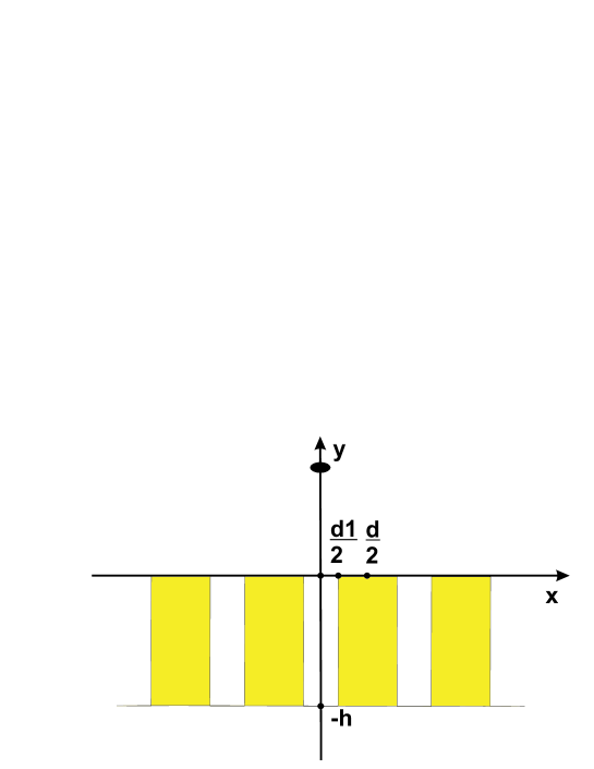
Figure 1: An atom (black ellipse) at position $(0,y,z)$ above a one-dimensional rectangular grating.

The grating displays a periodic surface profile $f(x)\in[-h,0]$ in the $x$-direction with period $d$, $f(x+d)=f(x)$ and height $h$ while being translationally invariant in the $z$-direction. To construct the Green’s tensor, we employ a plane-wave basis which is adapted to the symmetry of the system. Wave vectors for upward (+) and downward (-) moving waves are parametrised as $\bm{k}_{\pm}=(k_{x}^{m},\pm k_{y}^{m},k_{z})$. Their $x$-components are decomposed according to $k_{x}^{m}=k_{x}+mq$ into a continuous part $k_{x}\in[-q/2,q/2]$ that lies within the first Brillouin zone and a discrete part comprised of integer multiples $m\in\mathbb{Z}$ of the reciprocal lattice vector $q=2\pi/d$. The $z$-component takes arbitrary continuous values $k_{z}\in\mathbb{R}$ while the $y$-component then follows from the dispersion relation:

$$k_{y}^{m}=k_{y}^{m}(k_{x},k_{z},\omega)=\lim_{\delta\to 0_{+}}\sqrt{\frac{\omega^{2}}{c^{2}}\,(1+\mathrm{i}\delta)-(k_{x}^{m})^{2}-k_{z}^{2}}\quad\mbox{with }\operatorname{Im}k_{y}^{m}>0.$$ (1)

For each such wave vector $\bm{k}_{\pm}=\bm{k}_{m\pm}(k_{x},k_{z},\omega)$, we choose two perpendicular polarisation vectors $\bm{e}_{m\pm}^{E}$ and $\bm{e}_{m\pm}^{H}$ such that only the respective electric and magnetic fields exhibit non-vanishing $y$-components, respectively:

$$\bm{e}_{m\pm}^{E}(k_{x},k_{z},\omega)=\frac{c}{\omega\sqrt{\omega^{2}/c^{2}-k_{z}^{2}}}\begin{pmatrix}-k_{x}^{m}k_{z}\\ \mp k_{y}^{m}k_{z}\\ \omega^{2}/c^{2}-k_{z}^{2}\end{pmatrix}\,,$$ (2)

$$\bm{e}_{m\pm}^{H}(k_{x},k_{z},\omega)=\frac{1}{\sqrt{\omega^{2}/c^{2}-k_{z}^{2}}}\begin{pmatrix}\mp k_{y}^{m}\\ k_{x}^{m}\\ 0\end{pmatrix}\,.$$ (3)

These vectors are obviously normalised, $\bm{e}_{m\pm}^{E}\!\cdot\!\bm{e}_{m\pm}^{E}=\bm{e}_{m\pm}^{H}\!\cdot\!\bm{e}_{m\pm}^{H}=1$ and orthogonal to each other, $\bm{e}_{m\pm}^{E}\!\cdot\!\bm{e}_{m\pm}^{H}=0$, as well as to the unit wave vector $\bm{e}_{\bm{k}\pm}=\bm{k}_{\pm}/|\bm{k}_{\pm}|$, $\bm{e}_{m\pm}^{E}\!\cdot\!\bm{e}_{\bm{k}\pm}=\bm{e}_{m\pm}^{H}\!\cdot\!\bm{e}_{\bm{k}\pm}=0$. The three orthonormal vectors form a right-handed triad, $\bm{e}_{m\pm}^{H}\!\times\!\bm{e}_{m\pm}^{E}=\bm{e}_{\bm{k}\pm}$.

With these preparations at hand, the required scattering Green’s tensor can be given as

$$\mbox{{{{G}}}}^{(1)}(\bm{r},\bm{r}^{\prime},\omega)=\frac{\mathrm{i}}{8\pi^{2}}\int_{-q/2}^{q/2}\mathrm{d}k_{x}\sum_{m,n=-\infty}^{\infty}\int_{-\infty}^{\infty}\mathrm{d}k_{z}\sum_{\sigma,\sigma^{\prime}=E,H}\\ \times\frac{\mathrm{e}^{\mathrm{i}[k_{x}^{m}x-k_{x}^{n}x^{\prime}+k_{y}^{m}y+k_{y}^{n}y^{\prime}+k_{z}(z-z^{\prime})]}}{k_{y}^{n}}\,\bm{e}_{m+}^{\sigma}R_{mn}^{\sigma\sigma^{\prime}}\bm{e}_{n-}^{\sigma^{\prime}}.$$ (4)

The Rayleigh reflection coefficients $R_{mn}^{\sigma\sigma^{\prime}}=R_{mn}^{\sigma\sigma^{\prime}}(k_{x},k_{z},\omega)$ conserve $k_{x}$ and $k_{z}$ of the incident wave, but they mix polarisations $\sigma,\sigma^{\prime}$ as well as diffraction orders $m,n$ [20, 21]. In general, they have to be calculated numerically by integrating the Maxwell equations within the grating ($-h<y<0$) and imposing conditions of continuity at its upper and lower boundaries [3, 4, 5, 9]. For a rectangular grating (Fig. 1), the formalism for computing the Rayleigh coefficients is presented in Appendix A. Rayleigh reflection coefficients for a rectangular grating. Before we proceed, let us derive some symmetry properties of the reflection coefficients as well as consider the asymptotes of small and large grating periods.

2.1 Symmetry properties

Schwarz reflection principle. Like every causal response function, the scattering Green’s tensor obeys the Schwarz reflection principle $\mbox{{{{G}}}}^{(1)}(\bm{r},\bm{r}^{\prime},-\omega^{\ast})$ $=\mbox{{{{G}}}}^{(1)\ast}(\bm{r},\bm{r}^{\prime},\omega)$ [1]. Applying this to Eq. (4) leads to

$$R_{-m-n}^{\sigma\sigma^{\prime}}(-k_{x},-k_{z},-\omega^{\ast})=R_{mn}^{\sigma\sigma^{\prime}\ast}(k_{x},k_{z},\omega).$$ (5)

Onsager reciprocity. Provided that the grating consists of a medium which obeys time-reversal symmetry [22], the scattering Green’s tensor fulfils Onsager reciprocity $\mbox{{{{G}}}}^{(1)}(\bm{r}^{\prime},\bm{r},\omega)=\mbox{{{{G}}}}^{(1){\operatorname{T}}}(\bm{r},\bm{r}^{\prime},\omega)$. This implies

$$\frac{R_{-n-m}^{\sigma\sigma^{\prime}}(-k_{x},-k_{z},\omega)}{k_{y}^{m}}=\pm\frac{R_{mn}^{\sigma^{\prime}\sigma}(k_{x},k_{z},\omega)}{k_{y}^{n}}\quad\mbox{for }\sigma=\sigma^{\prime},\sigma\neq\sigma^{\prime}.$$ (6)

Grating symmetries. Finally, we consider symmetries imposed by the geometry of the grating. The invariance of the grating with respect to an inversion of the $z$ coordinate implies that the diagonal/off-diagonal Rayleigh coefficients are even/odd functions of $k_{z}$, respectively:

$$R_{mn}^{\sigma\sigma^{\prime}}(k_{x},-k_{z},\omega)=\pm R_{mn}^{\sigma\sigma^{\prime}}(k_{x},k_{z},\omega)\quad\mbox{for }\sigma=\sigma^{\prime},\sigma\neq\sigma^{\prime}.$$ (7)

For a symmetric grating with $f(-x)=f(x)$, we further have

$$R_{-m-n}^{\sigma\sigma^{\prime}}(-k_{x},k_{z},\omega)=\pm R_{mn}^{\sigma\sigma^{\prime}}(k_{x},k_{z},\omega)\quad\mbox{for }\sigma=\sigma^{\prime},\sigma\neq\sigma^{\prime}$$ (8)

by virtue of the $x$-inversion symmetry.

Further symmetries can be obtained by combining the above. For instance, Eqs. (5) and (6) imply $R_{nm}^{\sigma\sigma^{\prime}\ast}(k_{x},k_{z},\mathrm{i}\xi)/k_{y}^{m}=\pm R_{mn}^{\sigma^{\prime}\sigma}(k_{x},k_{z},\mathrm{i}\xi)/k_{y}^{n}$ for $\sigma=\sigma^{\prime},\sigma\neq\sigma^{\prime}$ at purely imaginary frequencies $\omega=\mathrm{i}\xi$.

2.2 Asymptotes

The exponential factors $\mathrm{e}^{\mathrm{i}k_{y}^{m}y}$ and $\mathrm{e}^{\mathrm{i}k_{y}^{n}y^{\prime}}$ become either exponentially damped or rapidly oscillating whenever $|k_{y}^{m}|y>1$ or $|k_{y}^{n}|y^{\prime}>1$, respectively. In the limit where the grating period is small with respect to the distances of source and field points from the grating, $d\ll y,y^{\prime}$, this implies that the Rayleigh sums in Eq. (4) are effectively limited to small values. To leading order $m=n=0$, we have

$$\mbox{{{{G}}}}^{(1)}(\bm{r},\bm{r}^{\prime},\omega)=\frac{\mathrm{i}}{8\pi^{2}}\int_{-q/2}^{q/2}\mathrm{d}k_{x}\,\mathrm{e}^{\mathrm{i}k_{x}(x-x^{\prime})}\int_{-\infty}^{\infty}\mathrm{d}k_{z}\frac{\mathrm{e}^{\mathrm{i}k_{y}^{0}(y+y^{\prime})+\mathrm{i}k_{z}(z-z^{\prime})}}{k_{y}^{0}}\\ \times\sum_{\sigma,\sigma^{\prime}=E,H}\bm{e}_{0+}^{\sigma}R_{00}^{\sigma\sigma^{\prime}}\bm{e}_{0-}^{\sigma^{\prime}}\\ =\frac{\mathrm{i}}{8\pi^{2}}\int_{-q/2}^{q/2}\mathrm{d}k_{x}\int_{-\infty}^{\infty}\mathrm{d}k_{z}\,\frac{\mathrm{e}^{2\mathrm{i}k_{y}^{0}y}}{k_{y}^{0}}\sum_{\sigma,\sigma^{\prime}=E,H}\bm{e}_{0+}^{\sigma}R_{00}^{\sigma\sigma^{\prime}}\bm{e}_{0-}^{\sigma^{\prime}}$$ (9)

in the coincidence limit $\bm{r}=\bm{r}^{\prime}$. This asymptote of the scattering Green’s tensor is thus translationally invariant along the $x$-direction and it is described by the effective properties of the grating averaged over one period. The leading correction to this $x$-independent Green’s tensor is a harmonic variation in $qx$ which is due to terms $m=0,n=\pm 1$ and $n=0,m=\pm 1$. In particular for a symmetric grating, this correction is proportional to $\cos(qx)$ in the coincidence limit.

In the opposite extreme of the grating period being very large with respect to the distances of source and field points from the grating, $d\gg y,y^{\prime}$, very large Rayleigh reflection orders $m,n\gg 1$ contribute. We thus have $k_{x}^{m}\approx mq$, $k_{y}^{m}(k_{x},k_{z},\omega)\approx k_{y}^{m}(0,k_{z},\omega)$, so that the polarisation unit vectors and reflection coefficients can be approximated by $\bm{e}_{m\pm}^{\sigma}(k_{x},k_{z},\omega)\approx$ $\bm{e}_{m\pm}^{\sigma}(0,k_{z},\omega)$ and $R_{mn}^{\sigma\sigma^{\prime}}(k_{x},k_{z},\omega)\approx R_{mn}^{\sigma\sigma^{\prime}}(0,k_{z},\omega)$. Carrying out the remaining $k_{x}$-integral, the scattering Green’s tensor assumes the asymptotic form

$$\mbox{{{{G}}}}^{(1)}(\bm{r},\bm{r}^{\prime},\omega)\simeq\frac{\mathrm{i}\sin[\pi(x-x^{\prime})/d]}{4\pi^{2}(x-x^{\prime})}\sum_{m,n=-\infty}^{\infty}\mathrm{e}^{\mathrm{i}q(mx-nx^{\prime})}\\ \times\int_{-\infty}^{\infty}\mathrm{d}k_{z}\frac{\mathrm{e}^{\mathrm{i}(k_{y}^{m}y+k_{y}^{n}y^{\prime})+\mathrm{i}k_{z}(z-z^{\prime})}}{k_{y}^{n-}}\sum_{\sigma,\sigma^{\prime}=E,H}R_{mn}^{\sigma\sigma^{\prime}}\bm{e}_{m+}^{\sigma}\bm{e}_{n-}^{\sigma^{\prime}}.$$ (10)

In the coincidence limit, the scattering Green’s tensor is then well described by a proximity force approximation [23, 24] where the grating is replaced by the local surface at $x=x^{\prime}$.

3 Casimir–Polder potential above a surface with one-dimensional periodic profile

Within leading-order perturbation theory, the CP potential of a ground-state atom within an arbitrary structure is given as [25]

$$U(\bm{r})=\frac{\hbar\mu_{0}}{2\pi}\int_{0}^{\infty}\mathrm{d}\xi\,\xi^{2}\mathrm{Tr}[\bm{\alpha}(\mathrm{i}\xi)\!\cdot\!\mbox{{{{G}}}}^{(1)}(\bm{r},\bm{r},\mathrm{i}\xi)],$$ (11)

where

$$\bm{\alpha}(\omega)=\lim_{\epsilon\to 0+}\frac{1}{\hbar}\sum_{k}\biggl{(}\frac{\bm{d}_{k0}\bm{d}_{0k}}{\omega+\omega_{k}+\mathrm{i}\epsilon}-\frac{\bm{d}_{0k}\bm{d}_{k0}}{\omega-\omega_{k}+\mathrm{i}\epsilon}\biggr{)}\;$$ (12)

is the ground-state polarisability of the atom as given in terms of its transition frequencies $\omega_{k}=(E_{k}-E_{0})/\hbar$ and dipole matrix elements $\bm{d}_{mn}$. Using the Green’s tensor (4) from the previous section, we find the CP potential of an atom above a one-dimensional grating as

$$U(\bm{r})=\frac{\hbar\mu_{0}}{16\pi^{3}}\int_{0}^{\infty}\mathrm{d}\xi\,\xi^{2}\int_{-q/2}^{q/2}\mathrm{d}k_{x}\sum_{m,n=-\infty}^{\infty}\mathrm{e}^{\mathrm{i}q(m-n)x}\int_{-\infty}^{\infty}\mathrm{d}k_{z}\,\frac{\mathrm{e}^{-(\kappa_{m}+\kappa_{n})y}}{\kappa_{n}}\\ \times\sum_{\sigma,\sigma^{\prime}=E,H}R_{mn}^{\sigma\sigma^{\prime}}\bm{e}_{m+}^{\sigma}\!\cdot\!\bm{\alpha}(\mathrm{i}\xi)\!\cdot\!\bm{e}_{n-}^{\sigma^{\prime}}$$ (13)

with $R_{mn}^{\sigma\sigma^{\prime}}=R_{mn}^{\sigma\sigma^{\prime}}(k_{x},k_{z},\mathrm{i}\xi)$ and

$$\kappa_{m}=\kappa_{m}(k_{x},k_{z},\mathrm{i}\xi)=\sqrt{\frac{\xi^{2}}{c^{2}}+(k_{x}^{m})^{2}+k_{z}^{2}}\,.$$ (14)

In the limit $d\ll y$ of small grating period, we use the asymptote (9) of the Green’s tensor to find the $x$-independent potential

$$U(\bm{r})=\frac{\hbar\mu_{0}}{16\pi^{3}}\int_{0}^{\infty}\mathrm{d}\xi\,\xi^{2}\int_{-q/2}^{q/2}\mathrm{d}k_{x}\int_{-\infty}^{\infty}\mathrm{d}k_{z}\,\frac{\mathrm{e}^{-2\kappa_{0}y}}{\kappa_{0}}\\ \times\sum_{\sigma,\sigma^{\prime}=E,H}R_{00}^{\sigma\sigma^{\prime}}\bm{e}_{0+}^{\sigma}\!\cdot\!\bm{\alpha}(\mathrm{i}\xi)\!\cdot\!\bm{e}_{0-}^{\sigma^{\prime}}.$$ (15)

For large grating period $d\gg y$, Eq. (10) leads to

$$U(\bm{r})=\frac{\hbar\mu_{0}}{8\pi^{2}d}\int_{0}^{\infty}\mathrm{d}\xi\,\xi^{2}\sum_{m,n=-\infty}^{\infty}\mathrm{e}^{\mathrm{i}q(m-n)x}\int_{-\infty}^{\infty}\mathrm{d}k_{z}\,\frac{\mathrm{e}^{-(\kappa_{m}+\kappa_{n})y}}{\kappa_{n}}\sum_{\sigma,\sigma^{\prime}=E,H}R_{mn}^{\sigma\sigma^{\prime}}\\ \times\bm{e}_{m+}^{\sigma}\!\cdot\!\bm{\alpha}(\mathrm{i}\xi)\!\cdot\!\bm{e}_{n-}^{\sigma^{\prime}}$$ (16)

with $k_{x}=0$ taken in all expressions inside the integrand.

4 Casimir–Polder potential above a one-dimensional rectangular grating

We study a ground-state Rb atom above a rectangular Au grating as shown in Fig. 1. The grating consists of a periodic array of rectangular bars of height $h=20\,\mathrm{nm}$ and width $2\,\mu\mathrm{m}$ with separation $d_{1}=2\,\mu\mathrm{m}$, so that the grating period is $d=4\,\mu\mathrm{m}$. The atom–grating potential is derived by numerically integrating Eq. (13) with the Rayleigh coefficients as given in Appendix A. Rayleigh reflection coefficients for a rectangular grating.

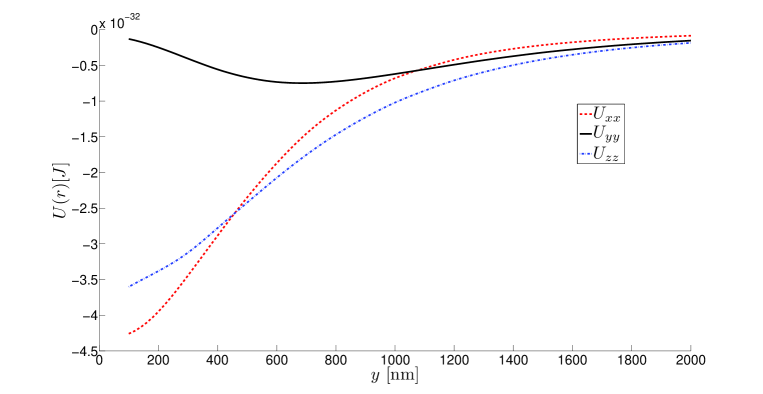
Figure 2: Contributions to the Casimir–Polder potential of a ground-state Rb atom above an Au grating as shown in Fig. 1.

To study the effect of possible anisotropies on the potential, we separate the latter into contributions from $\alpha_{xx}(\omega)=\alpha_{yy}(\omega)=\alpha_{yy}(\omega)=\alpha(\omega)$ where $\alpha(\omega)$ is the ground-state polarisability of the Rb atom: $U(\bm{r})=U_{xx}(\bm{r})+$ $U_{yy}(\bm{r})+U_{yy}(\bm{r})$. The resulting potentials at $x=0$ are shown in Fig. 2. We find that the component $U_{yy}$ leads to a repulsive Casimir–Polder potential in normal direction at separations $y\lesssim 700\,\mathrm{nm}$. This is the first demonstration of a repulsive Casimir–Polder potential for a grating geometry.

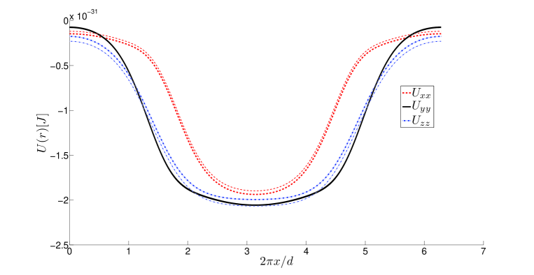
Figure 3: Casimir–Polder potential of a ground-state Rb atom at fixed distance $y=700$ nm above an Au grating as a function of lateral position. Thick lines: exact numerical results from Eq. (13). Thin lines: asymptotes from Eq. (16).

In many cases of interest, a full numerical calculation of the potential is neither desirable nor needed. For short atom-grating separations, the asymptotic expression (16) gives reliable results. In Fig. 3, we show a comparison of the full numerical calculation according to Eq. (13) (thick lines) with the short-distance asymptote (16) (thin lines) at a fixed atom-grating distance of $y=700\,\mathrm{nm}$. The obvious appearance of a non-sinusoidal lateral force across the grating implies in particular that the repulsive $U_{yy}$ component at $x=0$ leads to an unstable, saddle-point equilibrium in accordance with the generalised Earnshaw theorem [26]. One further notices that the short-distance (or large grating) approximation already provides very accurate results already at $y=700\,\mathrm{nm}$. At smaller separations of $y=300\,\mathrm{nm}$, the difference between exact and approximate potentials are within the thickness of the lines.

5 Conclusions

We have shown that it is possible to generate repulsive Casimir–Polder forces above material gratings using anisotropic atoms. Our calculation was based on the Green’s tensor expansion of the electromagnetic field which, using a Rayleigh expansion, yields both a numerically exact result as well as analytically tractable asymptotes for small and large gratings. Surprisingly, the short-distance (or large grating) asymptote becomes already accurate at a distance of $700\,\mathrm{nm}$ above a grating with a $4\,\mu\mathrm{m}$ period.

Appendix A. Rayleigh reflection coefficients for a rectangular grating

In the following, we determine the Rayleigh reflection coefficients for the rectangular grating depicted in Fig. 1. To this end, we express the electromagnetic fields above and below the grating for incident waves of polarisation $\sigma^{\prime}$ according to Eqs. (2) and (3) as (the factor $\mathrm{e}^{-\mathrm{i}\omega t+\mathrm{i}k_{z}z}$ is omitted for brevity)

$$E_{z}(x,y) = \mathrm{e}^{\mathrm{i}k_{x}^{m}x-\mathrm{i}k_{y}^{m}y}\delta_{E\sigma^{\prime}}+\sum_{n=-\infty}^{\infty}R_{nm}^{E\sigma^{\prime}}\mathrm{e}^{\mathrm{i}k_{x}^{n}x+\mathrm{i}k_{y}^{n}y},$$ (17)

$$H_{z}(x,y) = \mathrm{e}^{\mathrm{i}k_{x}^{m}x-\mathrm{i}k_{y}^{m}y}\delta_{H\sigma^{\prime}}+\sum_{n=-\infty}^{\infty}R_{nm}^{H\sigma^{\prime}}\mathrm{e}^{\mathrm{i}k_{x}^{n}x+\mathrm{i}k_{y}^{n}y}$$ (18)

for $y>0$ and

$$E_{z}(x,y) = \sum_{n=-\infty}^{\infty}T_{nm}^{E\sigma^{\prime}}\mathrm{e}^{\mathrm{i}k_{x}^{n}x-\mathrm{i}k_{y}^{n}y},$$ (19)

$$H_{z}(x,y) = \sum_{n=-\infty}^{\infty}T_{nm}^{H\sigma^{\prime}}\mathrm{e}^{\mathrm{i}k_{x}^{n}x-\mathrm{i}k_{y}^{n}y}$$ (20)

for $y<-h$, respectively. For simplicity, we take $c=1$ throughout this Appendix.

In the region $-h\leq y\leq 0$ one can write $E_{z}(x,y)=\sum_{n=-\infty}^{\infty}E_{z}^{n}(y)$ $\exp(\mathrm{i}k_{x}^{n}x)$, analogous decompositions hold for the other components of the electromagnetic field. It is convenient to denote by $[E]$ the $2N+1$-component vector with components $E_{N},E_{N-1},\dots,E_{0},\dots,E_{-N+1},E_{-N}$. We further introduce a diagonal $(2N+1)\times(2N+1)$-matrix

$$\Lambda={\rm diag}(k_{x}^{N},k_{x}^{N-1},\dots,k_{x}^{0},\dots,k_{x}^{-(N-1)},k_{x}^{-N}).$$ (21)

The Maxwell equations in the region $-h\leq y\leq 0$ can then be written as [21]

$$\frac{\partial[E_{z}]}{\partial y}-\mathrm{i}k_{z}[E_{y}]=\mathrm{i}\omega[H_{x}],\qquad \frac{\partial[H_{z}]}{\partial y}-\mathrm{i}k_{z}[H_{y}]=-\mathrm{i}\omega[D_{x}],$$ (22)

$$\mathrm{i}k_{z}[E_{x}]-i\Lambda[E_{z}]=\mathrm{i}\omega[H_{y}],\qquad \mathrm{i}k_{z}[H_{x}]-i\Lambda[H_{z}]=-\mathrm{i}\omega[D_{y}],$$ (23)

$$\mathrm{i}\Lambda[E_{y}]-\frac{\partial[E_{x}]}{\partial y}=\mathrm{i}\omega[H_{z}],\qquad \mathrm{i}\Lambda[H_{y}]-\frac{[H_{x}]}{\partial y}=-\mathrm{i}\omega[D_{z}].$$ (24)

Writing $[\bm{D}]=Q[\bm{E}]$ and using the results of Ref. [27], one has for a rectangular grating:

$$Q=\begin{pmatrix}\|\frac{1}{\varepsilon}\|^{-1}&0&0\\ 0&\|\varepsilon\|&0\\ 0&0&\|\varepsilon\|\end{pmatrix}.$$ (25)

Here, $\|\varepsilon\|$ is a Toeplitz matrix defined as

$$\|\varepsilon\|=\begin{pmatrix}\varepsilon_{0}&\varepsilon_{1}&\varepsilon_{2}&\dots&\varepsilon_{2N}\\ \varepsilon_{-1}&\varepsilon_{0}&\varepsilon_{1}&\dots&\varepsilon_{2N-1}\\ \varepsilon_{-2}&\varepsilon_{-1}&\varepsilon_{0}&\dots&\varepsilon_{2N-2}\\ \dots&\dots&\dots&\dots&\dots\\ \varepsilon_{-2N}&\varepsilon_{-2N+1}&\varepsilon_{-2N+2}&\dots&\varepsilon_{0}\end{pmatrix},$$ (26)

where $\varepsilon_{n}$ is a Fourier coefficient of the periodic function $\varepsilon(x+d)=\varepsilon(x)$:

$$\varepsilon(x)=\sum_{n=-\infty}^{+\infty}\exp\Bigl{(}\frac{i2\pi nx}{d}\Bigr{)}\varepsilon_{n}.$$ (27)

In order to solve the above system of equations, we proceed as follows. Equation (23) implies $[E_{y}]=\|\varepsilon\|^{-1}(\Lambda[H_{z}]-k_{z}[H_{x}])/\omega$, which can be substituted into equations (22) and (24) to eliminate $[E_{y}]$. Similarly, Eq. (23) leads to $[H_{y}]=(k_{z}[E_{x}]-\Lambda[E_{z}])/\omega$, which can be substituted into equations (22) and (24) to eliminate $[H_{y}]$. As a result, the Maxwell equations in the region $-h\leq y\leq 0$ can be rewritten as

$$\frac{\partial}{\partial y}\begin{pmatrix}[E_{x}]\\ [E_{z}]\\ [H_{x}]\\ [H_{z}]\end{pmatrix}=M\begin{pmatrix}[E_{x}]\\ [E_{z}]\\ [H_{x}]\\ [H_{z}]\end{pmatrix},$$ (28)

where the matrix $M$ is defined as

$$M=\mathrm{i}\begin{pmatrix}0&0&-\frac{k_{z}}{\omega}\Lambda\|\varepsilon\|^{-1}&\frac{1}{\omega}\Lambda\|\varepsilon\|^{-1}\Lambda-\omega I\\ 0&0&-\frac{k_{z}^{2}}{\omega}\|\varepsilon\|^{-1}+\omega I&\frac{k_{z}}{\omega}\|\varepsilon\|^{-1}\Lambda\\ \frac{k_{z}}{\omega}\Lambda&\omega\|\varepsilon\|-\frac{1}{\omega}\Lambda^{2}&0&0\\ \frac{k_{z}^{2}}{\omega}I-\omega\|\frac{1}{\epsilon}\|^{-1}&-\frac{k_{z}}{\omega}\Lambda&0&0\end{pmatrix}.$$ (29)

Knowing the transmitted fields (19) and (20) at $y=-h$, one can determine the fields at $y=0$ by integrating Eq. (28) from $-h$ to $0$. Imposing the continuity conditions on all Fourier components of $[E_{x}],[E_{z}],[H_{x}],[H_{z}]$ at $y=0$, one then determines the Rayleigh reflection and transmission coefficients.

References

• [1] S. Y. Buhmann, Dispersion Forces I: Macroscopic Quantum Electrodynamics and Ground-State Casimir, Casimir–Polder and van der Waals Forces (Springer, Heidelberg, 2012).
• [2] V. N. Marachevsky, J.Phys.A: Math.Theor. 45, 374021 (2012).
• [3] A. Lambrecht and V. N. Marachevsky, Phys. Rev. Lett. 101, 160403 (2008).
• [4] A. Lambrecht and V. N. Marachevsky, Int. J. Mod. Phys. A 24, 1789 (2009).
• [5] H.-C. Chiu, G. L. Klimchitskaya, V. N. Marachevsky, V. M. Mostepanenko and U. Mohideen, Phys. Rev. B 80, 121402(R) (2009); Phys. Rev. B 81, 115417 (2010).
• [6] R. B. Rodrigues, P. A. Maia Neto, A. Lambrecht and S. Reynaud, Phys. Rev. Lett. 96, 100402 (2006).
• [7] R. Messina, D. A. R. Dalvit, P. A. Maia Neto, A. Lambrecht and S. Reynaud, Phys. Rev. A 80, 022119 (2009).
• [8] A. M. Contreras-Reyes, R. Guérout, P. A. Maia Neto, D. A. R. Dalvit, A. Lambrecht and S. Reynaud, Phys. Rev. A 82, 052517 (2010).
• [9] H. Bender, C. Stehle, C. Zimmermann, S. Slama, J. Fiedler, S. Scheel, S. Y. Buhmann and V. N. Marachevsky, Phys. Rev. X 4, 011029 (2014).
• [10] R. Bennett, Phys. Rev. A 92, 022503 (2015).
• [11] M. Levin, A. P. McCauley, A. W. Rodriguez, M. T. H. Reid and S.G. Johnson, Phys. Rev. Lett. 105, 090403 (2010).
• [12] C. Eberlein and R. Zietal, Phys. Rev. A 83, 052514 (2011).
• [13] K. A. Milton, E. K. Abalo, P. Parashar, N. Pourtolami, I. Brevik and S. A. Ellingsen, J. Phys. A 45, 374006 (2012).
• [14] K. A. Milton, E. K. Abalo, P. Parashar, N. Pourtolami, I. Brevik, S. A. Ellingsen, S. Y. Buhmann and S. Scheel, Phys. Rev. A 91, 042510 (2015).
• [15] K. A. Milton, E. K. Abalo, P. Parashar, N. Pourtolami, I. Brevik and S. A. Ellingsen, Phys. Rev. A 83, 062507 (2011).
• [16] H. Failache, S. Saltiel, M. Fichet, D. Bloch, and M. Ducloy, Phys. Rev. Lett. 83, 5467 (1999).
• [17] S.Y. Buhmann and S. Scheel, Phys. Rev. Lett. 100, 253201 (2008).
• [18] P. S. Davids, F. Intravaia, F. S. S. Rosa and D. A. R. Dalvit, Phys. Rev. A 82, 062111 (2010).
• [19] S. Scheel and S. Y. Buhmann, Acta Phys. Slov. 58, 675 (2008).
• [20] O. M. Rayleigh, Proc. Roy. Soc. A. 79, 399 (1907).
• [21] D. Maystre (ed.) Selected Papers on Diffraction Gratings (SPIE, Bellingham, 1993); R. Petit (ed.), Electromagnetic Theory of Gratings (Springer-Verlag, Berlin, 1980); M. C. Hutley, Diffraction Gratings (Academic Press, London, 1982); E. G. Loewen and E. Popov, Diffraction Gratings and Applications (Marcel Dekker, New York, 1997).
• [22] S. Y. Buhmann, D. T. Butcher and S. Scheel, New J. Phys. 14, 083034 (2012).
• [23] B. V. Derjaguin, I. I. Abrikosova and E. M. Lifshitz, Q. Rev. Chem. Soc. 10, 295 (1956).
• [24] J. Błoccki, J. Randrup, W. J. Światecki and C. F. Tsang, Ann. Phys. 105, 427 (1977).
• [25] S. Y. Buhmann, L. Knöll, D.-G. Welsch and T. D. Ho, Phys. Rev. A 70, 052117 (2004).
• [26] S. J. Rahi, M. Kardar and T. Emig, Phys. Rev. Lett. 105, 070404 (2010).
• [27] L. Li, J. Opt. Soc. Am. A 13, 1870 (1996).