Apparent cross-field superslow propagation of magnetohydrodynamic waves in solar plasmas

Abstract

In this paper we show that the phase mixing of continuum Alfvén waves and/or continuum slow waves in magnetic structures of the solar atmosphere as, e.g., coronal arcades, can create the illusion of wave propagation across the magnetic field. This phenomenon could be erroneously interpreted as fast magnetosonic waves. The cross-field propagation due to phase mixing of continuum waves is apparent because there is no real propagation of energy across the magnetic surfaces. We investigate the continuous Alfvén and slow spectra in 2D Cartesian equilibrium models with a purely poloidal magnetic field. We show that apparent superslow propagation across the magnetic surfaces in solar coronal structures is a consequence of the existence of continuum Alfvén waves and continuum slow waves that naturally live on those structures and phase mix as time evolves. The apparent cross-field phase velocity is related to the spatial variation of the local Alfvén/slow frequency across the magnetic surfaces and is slower than the Alfvén/sound velocities for typical coronal conditions. Understanding the nature of the apparent cross-field propagation is important for the correct analysis of numerical simulations and the correct interpretation of observations.

1 Introduction

Recent numerical simulations of magnetohydrodynamic (MHD) waves in coronal arcades (Rial et al., 2010, 2013) and in the interior of prominences (Kaneko & Yokoyama, 2015, shown later) have revealed the presence of MHD waves propagating across the magnetic surfaces at slow velocities. It is standard to associate propagation across magnetic surfaces with fast magnetosonic MHD waves. However, the interpretation in terms of fast magnetosonic waves poses a problem since the apparent velocity of the cross-field propagation reported in those numerical studies is slower than that associated with a fast MHD wave and even a slow MHD wave. Here we show an example of cross-field superslow propagation. Figure. 1 (a) and (b) show snapshots at a certain time of the simulation in Kaneko & Yokoyama (2015), and Fig. 1 (c) shows the time evolution of the velocity component perpendicular to the plane along the slit in panel (a). In this simulation, radiative condensation happens at around time of 3000 s, and the waves are excited inside the flux rope. In Fig. 1 (c), at the region apart from the center of the flux rope (distance of 2–7 Mm) we clearly find waves which propagate outward and whose propagation speeds are decreasing with time. The propagation speeds are 1–5 km/s (as shown by dashed lines in panel (c)), much slower than the characteristic propagation speeds of the fast mode ($\sim$ 160 km/s in our simulation settings) and even the slow mode ($\sim$ 70 km/s). We think that the superslow propagation is explained as the apparent effect caused by phase mixing of standing Alfvén or slow waves trapped in the closed loops of the flux rope. In the present paper, as a first step, it is argued that in magnetic structures of the solar corona as, e.g., magnetic arcades, the phase mixing of continuum Alfvén waves and/or continuum slow waves can create the illusion of MHD waves propagating across magnetic surfaces at velocities smaller than the characteristic sound and Alfvén velocities of the plasma. This cross-field propagation is apparent because there is no real propagation of wave energy across the magnetic field.

Continuum Alfvén waves and continuum slow waves live on individual magnetic surfaces and are associated with the Alfvén continuum and slow continuum of the linear MHD spectrum (Appert et al., 1974). Each magnetic surface can oscillate at its own local Alfvén frequency and local slow frequency without interaction with neighbouring magnetic surfaces in ideal MHD and with negligible interaction in non-ideal MHD. If the continuum Alfvén/slow waves on a collection of neighbouring magnetic surfaces are excited each at their own local Alfvén/slow frequencies, an observer would see an apparent phase propagation across the magnetic surfaces due to the variation of the local Alfvén/slow frequency across those surfaces (Rial et al., 2010, 2013; Kaneko & Yokoyama, 2015). The apparent phase velocity is related to the spatial variation of the local Alfvén/slow frequency across the magnetic surfaces and is slower than the Alfvén/sound velocities for typical coronal conditions. The apparent propagation may be misleading for the analysis of simulations and observations, since this phenomenon could naturally be interpreted as fast MHD waves. Therefore, understanding the nature of the apparent wave propagation is important for the correct analysis of numerical simulations and the correct interpretation of observations.

Computations of the continuous spectrum that are relevant for the present investigation can be found in, e.g., Poedts & Goossens (1987, 1988, 1991), Oliver et al. (1993), Tirry & Poedts (1998), Arregui et al. (2004a, b) and Terradas et al. (2013). These investigations are concerned with 2D equilibrium models in Cartesian geometry that are invariant in the perpendicular direction to the 2D plane ($y$-direction). Poedts & Goossens (1987, 1988, 1991) computed the continuous spectrum of ideal MHD waves in 2D solar coronal loops and arcades. They dealt with equilibrium models with a purely poloidal magnetic field (Poedts & Goossens, 1987, 1988) and a mixed poloidal and toroidal magnetic field (Poedts & Goossens, 1991). They explicitly determined how the slow continuum frequencies and the Alfvén continuum frequencies change across the magnetic surfaces for specific choices of the magnetic field and equilibrium density. Oliver et al. (1993) computed the Alfvén continuous spectrum of a pressureless coronal arcade with a poloidal potential magnetic field. They neglected gravity and they removed the slow part of the spectrum by using the assumption that the plasma is pressureless. Tirry & Poedts (1998) studied MHD waves in potential arcades as Oliver et al. (1993). They determined the variation of the frequencies of Alfvén continuum modes across the magnetic surfaces for a specific density profile. Subsequently Tirry & Poedts (1998) studied the coupling of Alfvén continuum modes and fast modes in the resistive driven problem for $k_{y}\neq 0$, where $k_{y}$ denotes the wavenumber in the $y$-direction (the direction in the magnetic surfaces perpendicular to the magnetic field lines). Arregui et al. (2004a, b) studied MHD waves in potential arcades as Oliver et al. (1993) and in force free arcades. They determined the variation of the frequencies of Alfvén continuum modes across the magnetic surfaces for a specific density profile corresponding to $\delta=6$ in the notation of Oliver et al. (1993). They used their results on Alfvén continuum modes for a purely poloidal field and $k_{y}=0$ as starting point to understand the coupling of Alfvén continuum modes and fast waves in more complicated cases. Terradas et al. (2013) computed the slow and Alfvén continuum for a 2D prominence model with a purely poloidal magnetic field and gravity.

The aim of the present paper is to show that apparent superslow propagation across the magnetic surfaces in solar coronal structures is a consequence of the existence of continuum Alfvén waves and continuum slow waves. To this end we investigate the continuous spectrum for 2D equilibrium models in Cartesian geometry that are invariant in the $y$-direction and have a purely poloidal magnetic field. The actual equilibrium configurations that we have in mind are 2D coronal arcades (e.g. Oliver et al., 1993). The assumption that there is no toroidal magnetic field leads to two separate continuous parts. It simplifies the mathematical analysis and enables us to understand the essential mechanism behind the apparent superslow propagation.

The plan of the paper is as follows. In Section 2 we review the concept of continuous spectrum of linear ideal MHD and we recall the equations that govern the continuous spectrum for a 2D magnetostatic equilibrium in Cartesian coordinates with a purely poloidal magnetic field. In Section 3 we discuss the solutions for the Alfvén continuum waves and slow continuum waves. The apparent cross-field propagation caused by the phase mixing of continuum waves is studied in Section 4. In Section 5 we use the theory of apparent superslow propagation due to continuum Alfvén waves to explain the superslow propagation observed in the numerical simulations by Kaneko & Yokoyama (2015). Conclusions are formulated in Section 6.

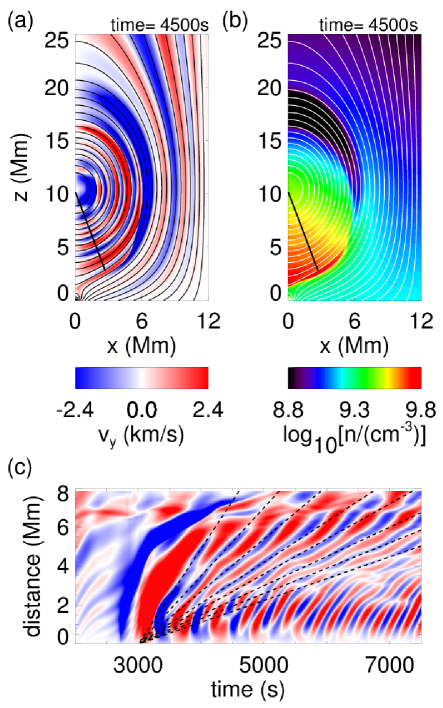
Figure 1: Superslow propagation in Kaneko & Yokoyama (2015). Panels (a) and (b) show the velocity component perpendicular to the plane and number density at a certain time, respectively. The thin solid lines represent magnetic field. The thick solid line is the slit. Panel (c) shows the time evolution of velocity component perpendicular to the plane along the slit in panel (a). The horizontal and vertical axes represent time and distance from the center of the flux rope, respectively.

2 The continuous spectrum

The continuous part of the linear spectrum of ideal MHD was first studied for 1D magnetostatic equilibrium models. Appert et al. (1974) were the first to give a rigorous proof that the linear spectrum of ideal MHD contains a continuous part. Their analysis applied to a 1D axisymmetric circular plasma cylinder, known in the plasma physics literature as the diffuse linear pinch. Waves belonging to the continuous part of the spectrum are recognized by their singular behaviour at a magnetic surface. In the case of a 1D magnetostatic equilibrium model (e.g. the plasma slab, the diffuse linear pinch) the linear MHD equations can be reduced to the classic Hain-Lust equation. The values of $\sigma^{2}$ that correspond to the mobile regular singular points of the Hain-Lust equation (Hain & Lust, 1958; Goedbloed & Hagebeuk, 1972) are associated with non-square integrable solutions and define two separate continuous parts of the spectrum, namely the Alfvén continuum and the cusp or slow continuum (see e.g. Goedbloed, 1983; Goedbloed & Poedts, 2004; Goossens, 1991; Sakurai et al., 1991; Goossens et al., 1992). The solutions that correspond to the Alfvén continuum and slow continuum are localized on the magnetic surfaces where the resonant conditions of the respective wave dispersion relations are satisfied. In addition they are characterized by motions in the magnetic surfaces respectively perpendicular and parallel to the magnetic field lines.

For 1D equilibrium models the determination of the frequencies of the continuous part of spectrum is relatively straightforward: put the coefficient function of the highest derivative in the Hain-Lust equation equal to zero. The resonant frequencies are given by simple algebraic relations. For 2D equilibrium models matters are more complicated. The equations for the linear motions are partial differential equations. The continuous spectrum is redefined as the collection of frequencies for which the solutions show non-square integrable singularities at a flux surface $\Psi=\Psi_{0}$. Pao (1975) and Goedbloed (1975) were the first to determine independently the equations that govern the continuous part of the linear ideal spectrum for 2D toroidal equilibrium configurations in the context of fusion plasma physics. They also derived basic properties of the continuous spectrum that do not depend on the details of the magnetic field. In particular they showed that in the general case of a mixed poloidal and toroidal magnetic field the Alfvén continuum and the cusp continuum become coupled and the continuum modes are no longer polarized purely parallel and purely perpendicular to the magnetic field lines. When the magnetic field is purely poloidal the Alfvén continuum and the slow continuum remain uncoupled and the continuum solutions are polarized as in the 1D case of the diffuse linear pinch.

In the astrophysical context, Poedts et al. (1985) and Goossens et al. (1985) derived the equations that govern the continuous spectrum for 2D equilibrium models in the presence of gravity. Poedts et al. (1985) considered a toroidal equilibrium model in cylindrical coordinates with invariance in the $\varphi$-direction. Goossens et al. (1985) used a Cartesian model with invariance in the $y$-direction. Poedts et al. (1985) and Goossens et al. (1985) confirmed the result known in fusion plasma physics that the two continua are coupled when the magnetic field has a component in the ignorable direction respectively $B_{\varphi}$ and $B_{y}$. In that situation both continua are affected by gravity. For a purely poloidal magnetic field the two continua are uncoupled and the corresponding solutions have the classic properties known from the analysis of the diffuse linear pinch. Here the Alfvén continuum is not affected by gravity, but the slow continuum is affected and it might be better referred to as the slow-gravity continuum. The singular solutions of the continuum Alfvén waves for 2D magnetostatic equilibrium models with a purely poloidal magnetic field were discussed in detail by Thompson & Wright (1993), Wright & Thompson (1994) and Tirry & Goossens (1995).

2.1 Continuous spectrum for a 2D equilibrium

In the present investigation we use the equations for the continuous part of the linear spectrum formulated by Goossens et al. (1985). These authors derived the equations that govern the continuous part of linear ideal MHD for 2D equilibrium configurations in Cartesian geometry that are invariant in the $y$-direction. The basic equations for the magnetostatic equilibrium and the linear motions superimposed on this equilibrium can be found in Section 2 of Goossens et al. (1985). We recall the necessary equations from Goossens et al. (1985) and add new information. The equilibrium quantities are functions of the Cartesian coordinates $x$ and $z$ but not of $y$. Goossens et al. (1985) implicitly specified the dependence on the ignorable coordinate $y$ and time $t$ as

$$\exp(ik_{y}y-i\sigma t)$$ (1)

with $k_{y}$ the wave number in the $y$-direction and $\sigma$ the frequency. It is standard practice to split the equilibrium magnetic field in a poloidal magnetic field $\mbox{\boldmath$B$}_{p}$ and a toroidal magnetic field $\mbox{\boldmath$B$}_{t}=B_{y}\mbox{\boldmath$1$}_{y}$. In the present paper we deal with equilibrium configurations with a purely poloidal magnetic field. In what follows $B_{y}=0$.

The poloidal magnetic field is written in terms of a magnetic flux function $\Psi(x,z)$ as

$$\mbox{\boldmath$B$}(x,z)=\mbox{\boldmath$B$}_{p}(x,z)=-\nabla\Psi(x,z)\times\mbox{\boldmath$1$}_{y}=\frac{\displaystyle\partial\Psi}{\displaystyle\partial z}\mbox{\boldmath$1$}_{x}-\frac{\displaystyle\partial\Psi}{\displaystyle\partial x}\mbox{\boldmath$1$}_{z}$$ (2)

where $\mbox{\boldmath$1$}_{x},\;\mbox{\boldmath$1$}_{y},\;\mbox{\boldmath$1$}_{z}$ are the unit vectors in the $x$-, $y$- and $z$-directions. The definition of $\mbox{\boldmath$B$}_{p}$ with the use of the flux function $\Psi$ implies that $\mbox{\boldmath$B$}_{p}\cdot\nabla\Psi=0$. Goossens et al. (1985) used a local system of flux coordinates $(\Psi,y,\chi)$ with $\chi$ the poloidal variable. All equilibrium variables are functions of $\Psi$ and $\chi$ but not of $y$. The equilibrium magnetic field has components $(0,0,B_{\chi})$ in the $(\Psi,y,\chi)$ system of coordinates. Expressions for the operators $\nabla,\nabla^{2},\mbox{div},\mbox{rot}$ can be found in Equations (7) - (10) of Goossens et al. (1985). The unit vector normal to the flux surfaces is $\mbox{\boldmath$1$}_{\Psi}$ and the unit vector in the magnetic surfaces parallel to the poloidal magnetic field is $\mbox{\boldmath$1$}_{\chi}$. For completeness, we note that $\mbox{\boldmath$1$}_{y}$ is the unit vector in the magnetic surfaces perpendicular to the poloidal magnetic field lines and $k_{y}$ is the wave number in the direction of $\mbox{\boldmath$1$}_{y}$. Hence $\mbox{\boldmath$1$}_{\chi}=\mbox{\boldmath$1$}_{\parallel},\;\;\mbox{\boldmath$1$}_{y}=\mbox{\boldmath$1$}_{\perp}$.

The local system of flux coordinates is orthogonal so that $\nabla\chi\cdot\nabla\Psi=0$. Hence

$$\nabla\chi=\lambda(x,z)\mbox{\boldmath$B$}_{p}$$ (3)

with $\lambda(x,z)$ a function that we can choose freely. The Jacobian $J$ of the transformation of the Cartesian system of coordinates $(x,y,z)$ to that of the local system of orthogonal flux coordinates $(\Psi,y,\chi)$ and the elementary length in the local system of orthogonal flux coordinates are

$$J = \frac{1}{\displaystyle B_{\chi}\mid\nabla\chi\mid}$$ (4)

$$(ds)^{2} = \frac{\displaystyle 1}{\displaystyle B_{\chi}^{2}}(d\Psi)^{2}+(dy)^{2}+J^{2}B_{\chi}^{2}(d\chi)^{2}$$ (5)

We use Equations (59)-(60) of Goossens et al. (1985). They are two uncoupled ordinary differential equations for respectively $\xi_{y}$ and $\xi_{\chi}$ on a given magnetic surface $\Psi=\Psi_{0}$. The independent variable is the coordinate along the field line, $\chi$. The actual equilibrium configurations that we have in mind are 2D arcades as studied by Poedts & Goossens (1987, 1988, 1991); Oliver et al. (1993); Tirry & Poedts (1998); Arregui et al. (2004b, b); Rial et al. (2010, 2013) and Terradas et al. (2013). A graphical representation of the magnetostatic configuration can be found in (Oliver et al., 1993) and Rial et al. (2010). Equations (59) - (60) of Goossens et al. (1985) are

$$\sigma^{2}\xi_{y} = -\frac{1}{\mu\rho_{0}}(F^{2})\;\xi_{y}$$ (6)

$$\sigma^{2}\xi_{\chi} = \left\{\frac{\displaystyle v_{S}^{2}}{\displaystyle v_{S}^{2}+v_{A}^{2}}N_{\chi}^{2}+\frac{\displaystyle 1}{\displaystyle JB_{\chi}^{2}}\frac{\displaystyle\partial}{\displaystyle\partial\chi}\left(\frac{\displaystyle v_{S}^{2}}{\displaystyle v_{S}^{2}+v_{A}^{2}}\frac{\displaystyle 1}{\displaystyle J}\frac{\displaystyle\partial\Phi_{0}}{\displaystyle\partial\chi}\right)\right\}\xi_{\chi},$$ (7)

$$- \frac{1}{\displaystyle\rho_{0}B_{\chi}}F\left\{\rho_{0}\;v_{C}^{2}\;F\left(\frac{\displaystyle\xi_{\chi}}{\displaystyle B_{\chi}}\right)\right\},$$

The operator $F$ is given by

$$F=\frac{\displaystyle 1}{\displaystyle J}\frac{\displaystyle\partial}{\displaystyle\partial\chi}.$$ (8)

Note that Goossens et al. (1985) used the notation $F^{\star}$ in stead of $F$. In these equations, $\rho_{0},p_{0},\Phi_{0}$ are the equilibrium density, pressure, and gravitational potential. In turn, $v_{S}^{2},$ $v_{A}^{2}$, and $v_{C}^{2}$ are the square of the local speed of sound, the local Alfvén velocity, and the local cusp (or tube) speed defined as

$$v_{S}^{2}=\frac{\displaystyle\gamma p_{0}}{\displaystyle\rho_{0}},\;\;v_{A}^{2}=\frac{\displaystyle B^{2}}{\displaystyle\mu\rho_{0}},\;\;v_{C}^{2}=\frac{\displaystyle v_{A}^{2}\;v_{S}^{2}}{\displaystyle v_{A}^{2}+v_{S}^{2}},\\$$ (9)

where $\gamma$ is the adiabatic index and $\mu$ is the magnetic permeability. $N_{\chi}^{2}$ is the square of the Brunt-Vaisälä frequency along the magnetic field lines. It is defined as

$$N_{\chi}^{2}=-\frac{\displaystyle 1}{\displaystyle JB_{\chi}}\frac{\displaystyle\partial\Phi_{0}}{\displaystyle\partial\chi}\left\{\frac{\displaystyle 1}{\displaystyle JB_{\chi}}\frac{\displaystyle 1}{\displaystyle\rho_{0}}\frac{\displaystyle\partial\rho_{0}}{\partial\chi}-\frac{\displaystyle 1}{\displaystyle\gamma p_{0}JB_{\chi}}\frac{\displaystyle\partial p_{0}}{\partial\chi}\right\}.$$ (10)

When equations (6) and (7) are supplemented with boundary conditions they define two uncoupled eigenvalue problems for the frequency, $\sigma$. When the magnetic surface is varied, the corresponding frequencies define respectively the Alfvén continuum and the cusp or slow continuum. Note that $\xi_{y}=\xi_{\perp}$ and $\xi_{\chi}=\xi_{\parallel}$. The equation for $\xi_{y}$ is independent of gravity and hence the Alfvén continuum is unaffected by gravity. The coefficient function of $\xi_{\chi}$ in the equation for $\xi_{\chi}$ clearly depends on gravity. Hence the slow continuum is affected by gravity. Note also that the wavenumber $k_{y}$ does not appear in Equations (6) and (7), so that the two continua are independent of $k_{y}$. The corresponding solutions spatially depend on $y$ through the factor $\exp(ik_{y}y)$.

2.2 Normalized variables

All the equations so far have been written in terms of dimensional variables. From here on we use normalized or dimensionless variables. We introduce a reference length $L_{R}$ and use it to define the normalized coordinates $x_{\star},y_{\star},z_{\star}$, the normalized arc length $s_{\star}$ and the normalized components of the Lagrangian displacement $\xi_{y,\star}\;\xi_{\chi,\star}$ as

$$[x,y,z]^{t}=L_{R}\;[x_{\star},y_{\star},z_{\star}]^{t},\;\;\;\;s=L_{R}\;s_{\star},\;\;\;[\xi_{y},\xi_{\chi}]^{t}=L_{R}\;[\xi_{y\star},\;\;\;\xi_{\chi\star}]^{t}$$ (11)

The operator $\nabla$ is transformed as $\nabla=(1/L_{R})\;\nabla_{\star}$. Next we introduce the reference value $\Psi_{R}$ to normalize the magnetic flux function $\Psi$, the variable $\chi$ and the poloidal magnetic field $\mbox{\boldmath$B$}_{p}$ as

$$\Psi = \Psi_{R}\;\Psi_{\star}(x_{\star},\;y_{\star},\;z_{\star}),\;\chi=\Psi_{R}\;\chi_{\star}(x_{\star},\;y_{\star},\;z_{\star}),$$

$$\mbox{\boldmath$B$}_{p} = B_{R}\;\mbox{\boldmath$B$}_{p\star},\;\;B_{R}=\Psi_{R}/L_{R}.$$ (12)

Equation (3) is then

$$\nabla_{\star}\chi_{\star}=\lambda(x,z)\;\mbox{\boldmath$B$}_{p\star}$$ (13)

A convenient choice for the multiplicative function $\lambda(x,z)$ in (13) is $\lambda(x,z)=1/(\mid B_{\chi\star}(x,z)\mid)$ so that

$$\nabla_{\star}\;\chi_{\star}=\mbox{\boldmath$1$}_{B}=\mbox{\boldmath$1$}_{\chi},\;\mid\nabla_{\star}\chi_{\star}\mid=1,\;J=(1/B_{R}^{2})J_{\star},\;J_{\star}=\frac{1}{B_{\chi\star}}.$$ (14)

The expression (5) for the elementary length is in dimensionless variables

$$(ds_{\star})^{2}=\frac{\displaystyle 1}{\displaystyle B_{\chi\star}^{2}}(d\Psi_{\star})^{2}+(dy_{\star})^{2}+(d\chi_{\star})^{2}$$ (15)

Equation (15) tells us that for constant $\Psi_{\star}$ and constant $y_{\star}$

$$(ds_{\star})^{2}=(d\chi_{\star})^{2}.$$ (16)

Hence $\chi_{\star}=s_{\star}$ with $s_{\star}$ the normalized arc length along a poloidal field line. In addition (8) can be simplified to

$$F=\frac{B_{R}}{L_{R}}\;F_{\star},\;\;\;F_{\star}=B_{\chi\star}\frac{\displaystyle\partial}{\displaystyle\partial\chi_{\star}}=B_{\star}\frac{\displaystyle\partial}{\displaystyle\partial s_{\star}}.$$ (17)

The equilibrium density and equilibrium pressure $\rho_{0},\;p_{0}\;$ are normalized by the use of the reference values $\rho_{R}$ and $p_{R}$:

$$\rho_{0}=\rho_{R}\;\rho_{\star},\;\;p_{0}=p_{R}\;p_{\star}$$ (18)

The local Alfvén velocity $v_{A}$, the local speed of sound $v_{S}$ and the local cusp speed $v_{C}$ are normalized with the reference value for the local Alfvén speed $v_{AR}$

$$v^{2}_{AR}=B_{R}^{2}/(\mu\rho_{R}),\;(v_{A},v_{S},v_{C})=v_{AR}\;(v_{A\star},\;v_{S\star},\;v_{C\star})$$ (19)

Expressions for $v_{A\star},\;v_{S\star},\;v_{C\star}$ are

$$v^{2}_{A\star}=\frac{B_{\star}^{2}}{\rho_{\star}},\;\;v^{2}_{S\star}=\frac{\beta_{R}}{2}\frac{\gamma p_{\star}}{\rho_{\star}},\;\;\beta_{R}=\frac{p_{R}}{B^{2}_{R}/(2\mu)},\;\;v_{C\star}^{2}=\frac{\displaystyle v_{A\star}^{2}\;v_{S\star}^{2}}{\displaystyle v_{A\star}^{2}+v_{S\star}^{2}}$$ (20)

The equilibrium potential $\Phi_{0}$ is normalized as

$$\Phi_{0}=v^{2}_{AR}\;\Phi_{\star}$$ (21)

Finally all frequencies are normalized by use of the reference Alfvén frequency $\sigma_{AR}$ as

$$\sigma^{2}_{AR}=\frac{v_{AR}^{2}}{{L_{R}}^{2}},\;\;\;\sigma^{2}=\sigma^{2}_{AR}\sigma_{\star}^{2},\;\;\;N_{\chi}^{2}=\sigma^{2}_{AR}N_{\chi\star}^{2}$$ (22)

The dimensionless square of the Brunt-Vaisälä frequency $N_{\chi\star}^{2}$ is

$$N_{\chi\star}^{2}=-g_{\chi\star}\left\{\frac{\displaystyle 1}{\displaystyle\rho_{\star}}\frac{\displaystyle\partial\rho_{\star}}{\partial s_{\star}}+\frac{\displaystyle g_{\chi,\star}}{\displaystyle v_{S^{\prime}\star}^{2}}\right\}$$ (23)

$g_{\chi\star}$ is the dimensionless component of gravity along the field line

$$g_{\chi\star}=\frac{\displaystyle\partial\Phi_{\star}}{\displaystyle\partial s_{\star}},$$ (24)

From here on only normalized quantities will be used and there is no room for confusion. Hence we drop the subscript $\star$ for the sake of simplicity. Equations (6) and (7) for the Alfvén continuum waves and the slow continuum waves can then be rewritten as

$$\sigma^{2}\xi_{y} = -\frac{1}{\rho}(B\frac{\displaystyle\partial}{\displaystyle\partial s})\left\{B\frac{\displaystyle\partial\xi_{y}}{\displaystyle\partial s}\right\},$$ (25)

$$\sigma^{2}\xi_{\chi} = \left\{\frac{\displaystyle v_{S}^{2}}{\displaystyle v_{S}^{2}+v_{A}^{2}}\;N_{\chi}^{2}+\frac{\displaystyle 1}{\displaystyle B}\frac{\displaystyle\partial}{\displaystyle\partial s}\left(\frac{\displaystyle v_{S}^{2}}{\displaystyle v_{S}^{2}+v_{A}^{2}}B\;g_{\chi}\right)\right\}\xi_{\chi},$$ (26)

$$- \frac{1}{\displaystyle\rho}\frac{\partial}{\partial s}\left\{\rho\;v_{C}^{2}\;B\frac{\partial}{\partial s}\left(\frac{\displaystyle\xi_{\chi}}{\displaystyle B}\right)\right\}.$$

3 Continuum waves

3.1 Alfvén waves

The Alfvén continuum waves are governed by equation (25). It is an ordinary differential equation of second order for $\xi_{y}=\xi_{\perp}$. We have deliberately kept the notation with the partial derivative $\partial/\partial s$ to make it clear that we are on a given magnetic surface $\Psi=\Psi_{0}$. The continuum Alfvén waves live on individual magnetic surfaces and the motions are in the $y$-direction i.e. in the magnetic surfaces and perpendicular to the magnetic field lines. Let us rewrite equation (25) as

$$\frac{\displaystyle\partial^{2}\xi_{y}^{2}}{\displaystyle\partial s^{2}}+\frac{\displaystyle 1}{\displaystyle B}\frac{\displaystyle\partial B}{\displaystyle\partial s}\;\frac{\displaystyle\partial\xi_{y}}{\displaystyle\partial s}+\frac{\displaystyle\sigma^{2}}{\displaystyle v_{A}^{2}}\;\xi_{y}=0.$$ (27)

Equation (27) agrees with Equation (15) of Terradas et al. (2013), which was obtained from Equation (59) of Goossens et al. (1985). Equation (27) is defined on the field line $\Psi=\Psi_{0}$. Let us denote the length of the field line as $L(\Psi_{0})$ and impose the boundary conditions that the magnetic field lines of the arcade are anchored in the dense plasma of photosphere

$$\xi_{y,\Psi_{0}}(s=0)=\xi_{y,\Psi_{0}}(s=L(\Psi_{0}))=0.$$ (28)

The boundary conditions (28) were also used by Poedts & Goossens (1987, 1988, 1991); Oliver et al. (1993); Arregui et al. (2003, 2004a, 2004b) and Terradas et al. (2013). Equation (27) and boundary conditions (28) define an eigenvalue problem with eigenvalue $\sigma^{2}$ and eigenfunction $\xi_{y,\Psi_{0}}(s)$. There are infinitely many eigensolutions

$$\sigma^{2}_{A,n}(\Psi_{0}),\;\;\xi_{y,A,n,\Psi_{0}}(s).$$ (29)

The notation in (29) is as follows: the subscript $A$ refers to Alfvén waves, $\Psi_{0}$ refers to the fact that we are on the magnetic surface $\Psi=\Psi_{0}$. The number $n$ is related to the number of internal nodes of $\xi_{y}$ as function of $s$, i.e. along the field line. So, $n=1$ corresponds to the fundamental mode, with no internal nodes, $n=2$ to the first overtone, with one internal node, etc (see Poedts & Goossens, 1987, 1988; Arregui et al., 2003, 2004a, 2004b). When we change $\Psi_{0}$ from $\Psi_{B}$ to $\Psi_{E}$ each of the frequencies $\sigma^{2}_{A,n}(\Psi_{0})$ maps out a continuous range of Alfvén frequencies. Hence we have infinitely many Alfvén continua

$$\sigma^{2}_{A,n}(\Psi),\;\;\Psi_{B}\leq\Psi\leq\Psi_{E}$$ (30)

where we have used $\Psi$ in stead of $\Psi_{0}$.

Let us turn back to equation (29). In general it does not admit closed analytical solution. The reason is that the coefficient function of the first order derivative of $\xi_{y}$ in the left hand member of equation (29) is in general non-zero and the coefficient function of $\xi_{y}$ in the left hand member of equation (29) is in general non-constant. The coefficient function of the first order derivative of $\xi_{y}$ in the left hand member of equation (29) is zero only when the magnetic field strength does not vary along the field line, i.e. when $B$ is a flux function $B=B(\Psi)$. However, there are situations where the magnetic field strength does vary along the field line as e.g. in Poedts & Goossens (1987, 1988, 1991); Oliver et al. (1993); Arregui et al. (2003, 2004a, 2004b) and Terradas et al. (2013). The coefficient function of $\xi_{y}$ in the left hand member of equation (29) is constant if the Alfvén velocity $v_{A}$ is constant i.e. when $v_{A}$ is a flux function $v_{A}=v_{A}(\Psi)$. The combination of $B$ is a flux function $B=B(\Psi)$ and $v_{A}$ is a flux function $v_{A}=v_{A}(\Psi)$ implies that density $\rho$ is a flux function $\rho=\rho(\Psi)$. Again in general the equilibrium density is not a flux function as f.e. Poedts & Goossens (1987, 1988, 1991); Oliver et al. (1993) and Terradas et al. (2013). Hence, in general equation (29) must be numerically solved. There are of course exceptions.

Oliver et al. (1993) considered a coronal arcade model and were able to obtain closed analytical solutions for the eigenfrequencies and eigensolutions of continuum Alfvén waves by the use of a clever choice of a non-constant equilibrium magnetic field and a non-constant equilibrium density. As a means for comparison, let us consider the case that both the magnetic field strength $B$ and the equilibrium density $\rho$ are flux functions: $B=B(\Psi),\;\rho=\rho(\Psi)$. The equation (27) for continuum Alfvén waves can be simplified to

$$\frac{\displaystyle\partial^{2}\xi_{y}}{\displaystyle\partial s^{2}}+\frac{\displaystyle\sigma^{2}}{\displaystyle v_{A}^{2}}\;\xi_{y}=0$$ (31)

where now $\sigma^{2}/v_{A}^{2}$ is a flux function and independent of $s$. The solutions to equation (31) and boundary conditions (28) are

$$\sigma^{2}_{A,n}(\Psi_{0}) = \frac{\displaystyle n^{2}\pi^{2}}{\displaystyle L^{2}(\Psi_{0})}v_{A}^{2}(\Psi_{0})$$ (32)

$$\xi_{y,A,n,\Psi_{0}}(s) = \delta(\Psi-\Psi_{0})\sin\left(\frac{\displaystyle n\pi}{\displaystyle L(\Psi_{0})}\;s\right)$$ (33)

The continuum Alfvén frequencies are

$$\sigma_{A,n}(\Psi) = \frac{\displaystyle n\pi}{\displaystyle L(\Psi)}v_{A}(\Psi)$$ (34)

$$= k_{\chi}(\Psi)\;v_{A}(\Psi)$$

$k_{\chi}(\Psi)=n\pi/L(\Psi)$ is the local parallel wave number. Equation (34) or (32) defines infinitely many Alfvén continua since $n=1,2,3,\ldots$:

$$[\;\mbox{min}\left(\frac{\displaystyle n\pi}{\displaystyle L(\Psi)}v_{A}(\Psi)\right)\;\;;\;\;\mbox{max}\left(\frac{\displaystyle n\pi}{\displaystyle L(\Psi)}v_{A}(\Psi)\right)\;]$$ (35)

The number of nodes along the field line in the eigenfunction given by (33) is $n-1$. Hence, $n=1$ corresponds to the fundamental mode without any internal nodes, $n=2$ to the first overtone with one internal node, etc. Equation (34) is very reminiscent of the classic result for 1D equilibrium models with a straight field. For instance for the diffuse linear pinch with a constant straight field the Alfvén continuum frequencies are given by

$$\sigma_{A}(r)=k_{z}v_{A}(r)$$ (36)

with $k_{z}$ the axial wavenumber or parallel wavenumber and $v_{A}(r)$ the Alfvén velocity that depends on the radial coordinate $r$. Equation (34) is formally the same as the result in equation (25) of Arregui et al. (2003). In general there are deviations from the simple result (34) when we consider 2D equilibrium models. These deviations are due to the fact that $B$ and $\rho$ are not flux functions but vary along field lines.

Numerical results for Alfvén continuum frequencies for a magnetostatic equilibrium with a purely poloidal field are given by Poedts & Goossens (1987, 1988); Oliver et al. (1993); Arregui et al. (2003, 2004a, 2004b) and Terradas et al. (2013). Our main interest is in the frequency of the fundamental continuum mode and its variation across magnetic surfaces for different magnetostatic equilibrium models. Oliver et al. (1993) computed how the continuum Alfvén frequency varies across the magnetic surfaces for different density variations obtained by varying their parameter $\delta$, namely the ratio of the magnetic scale height to the density scale height. The value of $\delta$ controls the variation of the local Alfvén velocity with height. In their figure 2b Oliver et al. (1993) plot the variation of the frequency of the fundamental continuum Alfvén wave for different profiles of local Alfvén velocity $(\delta=1,2,3,4,6)$ as function of $x_{0}$. The parameter $x_{0}$ of Oliver et al. (1993) labels the magnetic surfaces and can be related to $\Psi$. Oliver et al. (1993) found that the variation of the frequency of the fundamental Alfvén wave across the magnetic surfaces depends on the value of $\delta$. For $\delta<3$ the frequency $\sigma_{A}$ is a strictly decreasing function of $x_{0}$

$$\forall x_{0}\in[0\;;\;1]\;:\;\frac{d\sigma_{A}}{dx_{0}}<0$$ (37)

However for $\delta\geq 3$ $\sigma_{A}$ is no longer a monotonous function of $x_{0}$. There is a critical point $x_{C}$ so that

$$\exists x_{C}\in[0\;;\;1]:\frac{d\sigma_{A}}{dx_{C}}=0$$

$$\forall x_{0}\in[0\;;\;x_{C}[\;:\;\frac{d\sigma_{A}}{dx_{0}}<0,\;\;\;\forall x_{0}\in]x_{C}\;;\;1]\;:\;\frac{d\sigma_{A}}{dx_{0}}>0$$ (38)

This behaviour of the frequency of the fundamental continuum Alfvén mode was confirmed by Tirry & Poedts (1998) for $\delta=3$ and by Arregui et al. (2004a) for $\delta=6$.

3.2 Slow waves

The slow continuum waves are governed by equation (26). It is an ordinary differential equation of second order for $\xi_{\chi}=\xi_{\parallel}$. Again we have kept the notation with the partial derivative $\partial/\partial s$ to make it clear that we are on a given magnetic surface $\Psi=\Psi_{0}$. The continuum slow waves live on individual magnetic surfaces and the motions are in the $\chi$ direction i.e. in the magnetic surfaces and parallel to the magnetic field lines. Let us rewrite rewrite equation (26) as

$$\frac{\displaystyle\partial^{2}\xi_{\chi}^{2}}{\displaystyle\partial s^{2}}+F(\Psi_{0},s)\;\frac{\displaystyle\partial\xi_{\chi}}{\displaystyle\partial s}+G(\Psi_{0},s)\;\xi_{\chi}=0$$ (39)

The functions $F(\Psi_{0},s)$ and $G(\Psi_{0},s)$ are

$$F(\Psi_{0},s) = \frac{\displaystyle 1}{\displaystyle\rho_{0}\;v_{C}^{2}}\frac{\displaystyle\partial(\rho_{0}\;v_{C}^{2})}{\partial s}-\frac{\displaystyle 1}{\displaystyle B}\frac{\displaystyle\partial B}{\partial s},$$

$$G(\Psi_{0},s) = \frac{\displaystyle\sigma^{2}}{\displaystyle v_{C}^{2}}-\frac{\displaystyle\partial}{\displaystyle\partial s}\left(\frac{\displaystyle 1}{\displaystyle B}\frac{\displaystyle\partial B}{\partial s}\right)-\frac{\displaystyle 1}{\displaystyle\rho_{0}\;v_{C}^{2}}\frac{\displaystyle\partial(\rho_{0}\;v_{C}^{2})}{\partial s}\frac{\displaystyle 1}{\displaystyle B}\frac{\displaystyle\partial B}{\partial s}$$ (40)

$$+\frac{\displaystyle g_{\chi}}{\displaystyle v_{A}^{2}}\;\left\{\frac{\displaystyle 1}{\displaystyle\rho_{0}}\frac{\displaystyle\partial\rho_{0}}{\partial s}+\frac{\displaystyle g_{\chi}}{\displaystyle v_{S}^{2}}\right\}-\frac{\displaystyle 1}{\displaystyle v_{C}^{2}}\frac{\displaystyle\partial}{\displaystyle\partial s}\left(\frac{\displaystyle v_{C}^{2}}{\displaystyle v_{S}^{2}}\right)g_{\chi}$$

$$-\frac{\displaystyle 1}{\displaystyle v_{S}^{2}}\left(g_{\chi}\frac{\displaystyle 1}{\displaystyle B}\frac{\displaystyle\partial B}{\partial s}+\frac{\displaystyle\partial g_{\chi}}{\partial s}\right).$$

Equation (39) and equation (40) agree with equations (12) - (14) of Terradas et al. (2013) when it is taken into account that $g_{\chi}$ of the present paper is equal to $-g_{s}$ of Terradas et al. (2013).

Equation (39) is defined on the field line $\Psi=\Psi_{0}$. Let us impose the boundary conditions

$$\xi_{\chi,\Psi_{0}}(s=0)=\xi_{\chi,\Psi_{0}}(s=L(\Psi_{0}))=0.$$ (41)

In the same way as for the continuum Alfvén waves Equation (39) and boundary conditions (41) define an eigenvalue problem with eigenvalue $\sigma^{2}$ and eigenfunction $\xi_{\chi,\Psi_{0}}(s)$. There are infinitely many eigensolutions

$$\sigma^{2}_{S,n}(\Psi_{0}),\;\;\xi_{\chi,S,n,\Psi_{0}}(s).$$ (42)

The notation in equation (42) is similar to that used for continuum Alfvén waves in equation (29). When we change $\Psi_{0}$ from $\Psi_{B}$ to $\Psi_{E}$ each of the frequecies $\sigma^{2}_{S,n}(\Psi_{0})$ maps out a continuous range of Alfvén frequecies. Hence we have infinitely many slow continua

$$\sigma^{2}_{S,n}(\Psi),\;\;\Psi_{B}\leq\Psi\leq\Psi_{E}.$$ (43)

Let us now turn back to equation (39). In general it does not admit closed analytical solutions. Also gravity is an ingredient that complicates simple mathematical analysis. Let us consider the case that gravity is absent. Equation (26) or (39) can then be simplified to

$$\sigma^{2}\xi_{\chi}=-\frac{1}{\displaystyle\rho}\frac{\partial}{\partial s}\left\{\rho\;v_{C}^{2}\;B\;\frac{\partial}{\partial s}\left(\frac{\displaystyle\xi_{\chi}}{\displaystyle B}\right)\right\}.$$ (44)

In general the equilibrium quantities $\rho,B,v_{S}^{2},v_{A}^{2},v_{C}^{2}$ are not flux functions and do also depend on $s$. As a means for comparison, we consider the case that the magnetic field strength $B$, the equilibrium density $\rho$ and the cusp velocity are flux functions: $B=B(\Psi),\;\rho=\rho(\Psi),\;v_{C}(\Psi)$. The condition that the density and the cusp velocity are flux functions implies that also pressure $p$ and temperature $T$ are flux functions : $p=p(\Psi),\;T=T(\Psi)$. Equation (44) for continuum slow waves can then be simplified to

$$\frac{\displaystyle\partial^{2}\xi_{\chi}^{2}}{\displaystyle\partial s^{2}}+\frac{\displaystyle\sigma^{2}}{\displaystyle v_{C}^{2}}\;\xi_{\chi}=0$$ (45)

where now $\sigma^{2}/v_{C}^{2}$ is a flux function and independent of $s$. Equation (45) is identical to equation (31) for continuum Alfvén waves with $v_{A}^{2}$ replaced with $v_{C}^{2}$. Hence we can repeat the analysis for continuum Alfvén waves from equation (33) up to (35). In particular the continuum slow frequencies are

$$\sigma_{S,n}(\Psi) = \frac{\displaystyle v_{S}}{\displaystyle\sqrt{v_{S}^{2}+v_{A}^{2}}}\sigma_{A,n}(\Psi)$$ (46)

$$= k_{\chi}(\Psi)\;v_{C}(\Psi)$$

The local parallel wave number $k_{\chi}(\Psi)$ is given by the same expression as for Alfvén waves (34). As for the Alfvén continuum we can refer to the classic result for 1D equilibrium models with a straight field. For instance for the diffuse linear pinch with a constant straight field the Alfvén continuum frequencies are given by

$$\sigma_{S}(r)=k_{z}v_{A}(r)$$ (47)

with $k_{z}$ the axial wavenumber or parallel wavenumber and $v_{A}(r)$ the Alfvén velocity that depends on the radial coordinate $r$. In general there are deviations from the simple result (46) when we consider 2D equilibrium models. These deviations are due to the fact that $\rho,B,v_{S}^{2},v_{A}^{2},v_{C}^{2}$ are not flux functions and also vary along the field lines and depend on $s$.

Numerical results for slow continuum frequencies for a magnetostatic equilibrium with a purely poloidal field are given by Poedts & Goossens (1987, 1988) and Terradas et al. (2013). In particular Poedts & Goossens (1988) show that the variation of the frequency of the slow continuum modes depends on the structure of the magnetic field, the density stratification and on the plasma beta $\beta$. The variation of the frequency of the slow continuum modes across the magnetic surfaces can be both monotonic and non-monotonic with a local minimum as can be seen in figure 4 of Poedts & Goossens (1988).

3.3 Closed magnetic surfaces

In this subsection, we consider waves on closed magnetic flux surfaces. These closed surfaces could correspond to the nested flux surfaces near the core of a prominence, which are detached from the lower atmospheric layers (at least in a 2D cut of the model, see e.g. the simulations in Kaneko & Yokoyama (2014, 2015)). For example, we can consider a magnetic field with flux surfaces that are concentric circular cylinders. Because of the assumed $y$-invariance of equilibrium configuration and in particular of the equilibrium magnetic field, we can concentrate on the $(x,z)$ plane. The intersections of the flux surfaces with the $(x,z)$ plane define concentric circular field lines with prescribed length $L(\Psi)=2\pi R(\Psi)$ where $L(\Psi)$ and $R(\Psi)$ denote the length of the circular field and its radius on each closed magnetic surface. Note that a possible magnetic field that satisfies the condition for magneto-static equilibrium is $B(\Psi)=B_{0}(R_{0}/R(\Psi))$. Otherwise, we need a pressure gradient in the radial direction for magneto-static equilibrium. On these closed flux surfaces different boundary conditions have to be considered, because Eq. (28) and (41) assume that the velocity perturbations are suppressed in a lower atmospheric layer with high inertia. The boundary conditions on closed magnetic surfaces are modified to

$$\xi_{y,\Psi_{0}}(s=0)=\xi_{y,\Psi_{0}}(s=L(\Psi_{0}))\quad\mbox{and}\quad\xi_{\chi,\Psi_{0}}(s=0)=\xi_{\chi,\Psi_{0}}(s=L(\Psi_{0})).$$ (48)

The difference is that the velocity components do not need to be zero at $s=0=L(\Psi_{0})$, but that the velocity components just need to be periodic functions of $s$, because the latter is a periodic coordinate as well.

Let us first focus on the Alfvén wave solutions, and let us once again consider that the magnetic field $B=B(\Psi)$ and the density $\rho=\rho(\Psi)$ are flux functions. As explained previously, the eigenvalue problem for Alfvén waves then reduces to Eq. (31):

$$\frac{\displaystyle\partial^{2}\xi_{y}}{\displaystyle\partial s^{2}}+\frac{\displaystyle\sigma^{2}}{\displaystyle v_{A}^{2}}\;\xi_{y}=0,$$ (49)

with boundary condition

$$\xi_{y,\Psi_{0}}(s=0)=\xi_{y,\Psi_{0}}(s=L(\Psi_{0})).$$ (50)

This is of course a well known problem, with a standard set of solutions. The general solution is

$$\xi_{y,\Psi_{0}}=\delta(\Psi-\Psi_{0})\left(\sum_{n^{\prime}=1}^{\infty}A_{n^{\prime}}\sin{\left(\frac{2\pi n^{\prime}}{L(\Psi_{0})}s\right)}+B_{n^{\prime}}\cos{\left(\frac{2\pi n^{\prime}}{L(\Psi_{0})}s\right)}\right),$$ (51)

where we have used the notation $n^{\prime}$ for half the number of nodes along the flux surface (and it is thus slightly different than the meaning in Subsect. 3.1 and 3.2). As expression for the Alfvén frequency continuum $\sigma_{A,n^{\prime}}$ we thus find

$$\sigma_{A,n^{\prime}}(\Psi)=\frac{2\pi n^{\prime}}{L(\Psi)}v_{A}(\Psi).$$ (52)

Analogously, one may derive the expression for the slow continuum and their eigenfunction in such a configuration of closed flux surfaces. As in Subsect. 3.2, the eigenfunction will have the same form as Eq. (51), but then for the $\xi_{\chi}$ component. Likewise, the continuum frequencies for the slow waves will be

$$\sigma_{A,n^{\prime}}(\Psi)=\frac{2\pi n^{\prime}}{L(\Psi)}v_{C}(\Psi).$$ (53)

4 Apparent cross-field propagation due to phase mixing of continuum waves

In this Section we show how the phase mixing of Alfvén/slow continuum waves creates the illusion of wave propagation across the magnetic surfaces. We stress that this cross-field propagation is not real and derive the apparent propagation phase velocity. Since the analysis is similar for Alfvén waves and slow waves, first we focus on the case of Alfvén waves and later we extend the results to slow waves.

Let us consider a situation where standing Alfvén continuum waves each with their own continuum frequency are excited on magnetic surfaces $\Psi_{B}\leq\Psi\leq\Psi_{E}$ with amplitude $A(\Psi)$ so that

$$\xi_{y}(\Psi,s,t)=A(\Psi)f_{A,\Psi}(s)\exp(i\sigma_{A}(\Psi)\;t).$$ (54)

The properties of perturbations with this form also occur in a magnetospheric context where they have been considered by Wright et al. (1999). We have dropped the subscript $n$ on $\sigma_{A}(\Psi)$. The function $f_{A,\Psi}$ is the solution of (27) for the corresponding continuum frequency $\sigma_{A}(\Psi)$ . In (54) we have assumed that there is no phase difference between the standing continuum Alfvén waves on different magnetic surfaces. Time $t$ in (54) is dimensionless. It is equal to dimensional real time multiplied with $\sigma_{A,R}$. The waves defined in (54) are standing in the $\chi$ direction and (apparently) propagating in the $\Psi$ direction. Let us now determine the apparent propagation of the phase in (54). The motion defined in (54) is multidimensional and its phase depends on position and on time. Its dependence on position is in general not linear. For a multidimensional wave with phase $\varphi(\mbox{\boldmath$x$},t)$ so that there is an exponential dependence

$$\exp(i\;\varphi(\mbox{\boldmath$x$},t)\;)$$ (55)

an instantaneous local frequency $\sigma$ and an instantaneous local wave vector $k$ can be defined as

$$\sigma=\frac{\displaystyle\partial\varphi(\mbox{\boldmath$x$},t)}{\displaystyle\partial\;t},\;\;\mbox{\boldmath$k$}=-\nabla\varphi(\mbox{\boldmath$x$},t).\;\;$$ (56)

Note that the wave vector $k$ is dimensionless. It is equal to the dimensional physical wave vector multiplied with $1/L_{R}$. A phase velocity can be defined in any direction (see e.g. Born & Wolf, 1999). We adopt the traditional version and choose the direction normal to the wave front i.e. the direction of $k$ so that

$$\mbox{\boldmath$v$}_{ph}=\frac{\displaystyle\sigma}{\displaystyle\mid\mbox{\boldmath$k$}\mid}\mbox{\boldmath$1$}_{k}.$$ (57)

Here $\varphi(\mbox{\boldmath$x$},t)=\sigma_{A}(\Psi)\;t$ so that the local frequency $\sigma$ defined in (56) is $\sigma_{A}(\Psi)$. The local wave number $k$ is

$$k = -t\;\nabla\sigma_{A}(\Psi)$$ (58)

$$= -t\;\frac{\displaystyle d\sigma(\Psi)}{\displaystyle d\Psi}\;\nabla\Psi$$

$$= -t\;\frac{\displaystyle d\sigma(\Psi)}{\displaystyle d\Psi}\;\mid\nabla\Psi\mid\mbox{\boldmath$1$}_{\Psi}$$

$$= -t\;\frac{\displaystyle d\sigma(\Psi)}{\displaystyle d\Psi}\;B(\Psi,\chi)\;\mbox{\boldmath$1$}_{\Psi}.$$

The last line of (58) follows from the fact that $\mid\nabla\Psi\mid\;=\;\mid\mbox{\boldmath$B$}_{p}(\Psi,\chi)\mid\;=\;B(\Psi,\chi)$. Equation (58) tells us that the phase vector $k$ is antiparallel to $\nabla\sigma_{A}(\Psi)$. Hence an increase /decrease in $\sigma_{A}(\Psi)$ with $\Psi$ corresponds to apparent downward/upward propagation

apparent upward propagation $$: \;\;\frac{\displaystyle d\sigma_{A}(\Psi)}{\displaystyle d\Psi}<0$$

apparent downward propagation $$: \;\;\frac{\displaystyle d\sigma_{A}(\Psi)}{\displaystyle d\Psi}>0$$ (59)

Equation (58) also shows that (1) $\mid\mbox{\boldmath$k$}\mid$ increases linearly in time generating scales that decrease inversely proportional to time $t$ (as was also found by Mann et al. (1995)), (2) $k$ has only a component in the $\Psi$-direction i.e. normal to the magnetic surfaces and (3) $\mbox{\boldmath$1$}_{k}=\pm\mbox{\boldmath$1$}_{\Psi}$ where the $\pm$ sign corresponds to $d\sigma_{A}(\Psi)/d\Psi<0,>0$. The phase velocity $\mbox{\boldmath$v$}_{ph}$ is

$$\mbox{\boldmath$v$}_{ph}=-\frac{\displaystyle 1}{\displaystyle t}\;\frac{\displaystyle\sigma_{A}(\Psi)}{\frac{\displaystyle d\sigma_{A}(\Psi)}{\displaystyle d\Psi}}\;\frac{\displaystyle 1}{\displaystyle B(\Psi,\chi)}\;\mbox{\boldmath$1$}_{\Psi}.$$ (60)

Equation (60) is a key result as it shows that there is an apparent propagation of phase when continuum Alfvén waves are excited on magnetic surfaces. There is apparent upward/downward propagation when $v_{ph}>0,\;\;v_{ph}<0$ which according to (60) happens when (59) applies. In general $k$ and $\mbox{\boldmath$v$}_{ph}$ are functions of $\Psi,\chi$ and time $t$. In case the magnetic field strength and the equilibrium density are flux functions we can rewrite equation (60) as

$$\mbox{\boldmath$v$}_{ph}=-\frac{\displaystyle 1}{\displaystyle t}\;\frac{\displaystyle 1}{\displaystyle\frac{\displaystyle 1}{\displaystyle v_{A}(\Psi)}\frac{\displaystyle dv_{A}(\Psi)}{\displaystyle d\Psi}-\frac{\displaystyle 1}{\displaystyle L(\Psi)}\frac{\displaystyle dL(\Psi)}{\displaystyle d\Psi}}\;\frac{\displaystyle 1}{\displaystyle B(\Psi)}\;\mbox{\boldmath$1$}_{\Psi}.$$ (61)

The condition for apparent upward/downward propagation (59) can now be rewritten as

upward propagation $$: \;\;\frac{\displaystyle 1}{\displaystyle v_{A}(\Psi)}\frac{\displaystyle dv_{A}(\Psi)}{\displaystyle d\Psi}<\frac{\displaystyle 1}{\displaystyle L(\Psi)}\frac{\displaystyle dL(\Psi)}{\displaystyle d\Psi}$$

downward propagation $$: \;\;\frac{\displaystyle 1}{\displaystyle v_{A}(\Psi)}\frac{\displaystyle dv_{A}(\Psi)}{\displaystyle d\Psi}>\frac{\displaystyle 1}{\displaystyle L(\Psi)}\frac{\displaystyle dL(\Psi)}{\displaystyle d\Psi}$$ (62)

Equivalent formulae to our equations (59)-(62) have been derived elsewhere and used to infer magnetospheric structure based upon the direction and speed of observed phase motion. The interested reader is directed to the summary given by Wright & Mann (2006). Regarding the closed magnetic field, the number of nodes can affect the phase velocity. When one particular node is dominant, Eq. (61) and the condition (62) are available without any modification (substitute Eq. (52) or (53) to Eq. (60)). If the multiple nodes exist on a magnetic surface, the appearance of the apparent propagation will become more complicated. It is straightforward to adapt the preceding analysis to include an initial phase difference between the excited Alfvén continuum waves. We denote the initial phase difference as $\varphi_{0}(\Psi)$. The expression (60) for the apparent propagation speed becomes

$$\mbox{\boldmath$v$}_{ph}=-\frac{\displaystyle\sigma_{A}(\Psi)}{t\frac{\displaystyle\;d\sigma_{A}(\Psi)}{\displaystyle d\Psi}+\frac{\displaystyle\;d\varphi_{0}(\Psi)}{\displaystyle d\Psi}}\;\frac{\displaystyle 1}{\displaystyle B(\Psi,\chi)}\;\mbox{\boldmath$1$}_{\Psi}.$$ (63)

Here, we present an example of upward and downward propagation by using a simple model. We consider the semicircular magnetic field described as

$$\mbox{\boldmath$B$}=\mbox{\boldmath$1$}_{\theta}~{}~{}(0<\theta<\pi),$$ (64)

where $\mbox{\boldmath$1$}_{\theta}$ is the unit vector in the $\theta$ direction in a system of polar coordinate in $(x,z)$ plane (see also the magnetic configuration in Fig. 2). In this particular case, the flux surface $\Psi=\Psi_{0}$ corresponds to $r=r_{0}$ due to the uniform unit field strength in the whole domain. The solution of the fundamental standing Alfvén wave on each flux surface $r$ is

$$\xi_{y}(r,\theta,t)=\sin\left(\sigma_{A}(r)t\right)\sin\theta,$$ (65)

where $\sigma_{A}(r)=2\pi v_{A}(r)/L(r)$ and $L(r)=\pi r$. Since the magnetic field is not force-free, a pressure gradient in the radial direction is required for magneto-static equilibrium. We do not concern here about pressure. Our focus is on continuum Alfvén waves and from the discussion in subsection 3.1 we recall that pressure has not any effect on the Alfvén continuum waves. The distribution of Alfvén velocity is set as

$$v_{A}(r)=\exp\left(\frac{r}{a}\right)$$ (66)

where $a=0.55$. In this setting, the wave vector and phase speed of apparent cross-field propagation are computed from Eqs. (58) and (61) as

$$k = -\frac{2t}{r}\left(\frac{1}{a}-\frac{1}{r}\right)\exp\left(\frac{r}{a}\right)\mbox{\boldmath$1$}_{r},$$ (67)

$$\mbox{\boldmath$v$}_{ph} = -\frac{1}{t}\frac{ar}{r-a}\mbox{\boldmath$1$}_{r}.$$ (68)

The condition for upward/downward propagation is

upward propagation $$: \;\;\frac{\displaystyle 1}{\displaystyle a}<\frac{\displaystyle 1}{\displaystyle r}$$

downward propagation $$: \;\;\frac{\displaystyle 1}{\displaystyle a}>\frac{\displaystyle 1}{\displaystyle r}$$ (69)

Hence, the condition for upward propagation is satisfied for the region with $r<a$ and that for downward propagation is satisfied in the region wit $r>a$. Figure. 2 shows the snapshots of the time evolution of the standing wave solution described as Eq. (65). Figure. 3 is the time-height plot along $x=0$ of Fig. 2. The dividing line between the regions of upward and downward propagation matches the criteria (69). It is also evident in Figs. 2 and 3 that the apparent wave vector increases with time as derived in Eq. (67), which is the nature of phase mixing. Moreover, the apparent phase speed is getting slower and slower as time goes on, which agrees with Eq. (68). If the standing waves are retained for a long time before they are dissipated by some instabilities or the local diffusivity during phase mixing, the phase speed is getting slower and slower, resulting in superslow propagation.

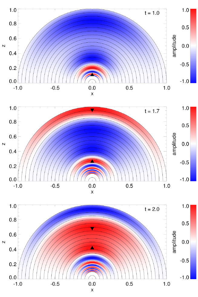
Figure 2: Snapshots of time evolution of Eq. (65). Color contour represents the amplitude orthogonal to the plane. Solid lines show the assumed magnetic field of Eq. (64). The triangles and inverse triangles mark the same phase ($\Phi=20.5$), and show the upward and downward propagation, respectively.

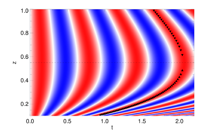
Figure 3: Time-height plot along $x=0$ of Fig. 2. Horizontal and vertical axis represents time $t$ and height $z$, respectively. Dashed line shows the border of upward and downward propagation derived by criteria (69). Color contour, triangles and inverse triangles represent the same meaning in Fig, 2.

Let us now go back to the coronal arcade model of Oliver et al. (1993). According to (58) and (59) it follows that the apparent propagation of the phase is always upward for models with $\delta<3$. For models with $\delta\geq 3$ the apparent propagation of phase is upward for $\forall x_{0}\in[0\;;\;x_{C}[$ and downward for $\forall x_{0}\in]x_{C}\;;\;1]$.

Figure 4: Magnetic field lines in the potential coronal arcade studied by Oliver et al. (1993). The magnetic field is given by $B_{x}=B_{0}\cos\left(x/\Lambda_{B}\right)e^{-z/\Lambda_{B}}$, $B_{z}=-B_{0}\sin\left(x/\Lambda_{B}\right)e^{-z/\Lambda_{B}}$, being $\Lambda_{B}=2L/\pi$ and $L$ half the arcade width. On each field line $\Psi$ is constant. The magnetic field lines can be identified by their footpoints, $x_{0}$, at $z=0$, or equivalently, by the value of $\Psi$.

Let us focus on a particular example that might be illustrative of the application of Equation (60). Oliver et al. (1993) found an analytic solution for the potential arcade (see Figure 4) with $\delta=0$. In this case these authors found that, for the fundamental mode with $n=0$, the dependence of the Alfvén frequency on the footpoint position ($x_{0}$) is

$$\sigma_{A}=\frac{\pi}{2x_{0}}v_{A0}\cos\left(x_{0}/\Lambda_{B}\right).$$ (70)

In this expression $v_{A0}=B_{0}/\sqrt{\mu\rho_{0}}$ is the Alfvén speed at $z=0$ and is independent of the $x-$coordinate.

Using the flux function it is straight forward to relate $\Psi$ with $x_{0}$, since

$$\Psi=-B_{0}\Lambda_{B}\cos\left(x\right/\Lambda_{B})e^{-z/\Lambda_{B}},$$ (71)

at $z=0$ we simply have that

$$\Psi=-B_{0}\Lambda_{B}\cos\left(x_{0}/\Lambda_{B}\right).$$ (72)

The next step is to evaluate the derivative of the Alfvén frequency with respect to $\Psi$. This is done using the fact that

$$\frac{d\sigma_{A}}{d\Psi}=\frac{d\sigma_{A}}{dx_{0}}\frac{dx_{0}}{d\Psi}.$$ (73)

Using Equations (70) and (72) we find

$$\frac{d\sigma_{A}}{d\Psi}=-\frac{\pi}{2x_{0}}v_{A0}\left[\frac{1}{x_{0}}\cos\left(x_{0}/\Lambda_{B}\right)+\frac{1}{\Lambda_{B}}\sin\left(x_{0}/\Lambda_{B}\right)\right]\frac{1}{B_{0}\sin\left(x_{0}/\Lambda_{B}\right)}.$$ (74)

Now we need the expression for $B(\Psi,\chi)$. Since it depends on the coordinate along the particular field line we concentrate at the position where it has a minimum and therefore the phase velocity has a maximum. This position is simply at $x=0$ in our arcade configuration, i.e., at the center of the arcade where there is only a horizontal component of the magnetic field. The horizontal component of the field line crossing the center of the arcade that has its footpoint at $x_{0}$ is $B_{0}\cos\left(x_{0}/\Lambda_{B}\right)$. Hence the phase velocity in the $z-$direction at the center of the arcade is

$$v_{phz}=\frac{1}{t}\frac{\sin\left(x_{0}/\Lambda_{B}\right)}{\frac{1}{x_{0}}\cos\left(x_{0}/\Lambda_{B}\right)+\frac{1}{\Lambda_{B}}\sin\left(x_{0}/\Lambda_{B}\right)}.$$ (75)

It is interesting to note that according to (75) the apparent phase speed, which is always pointing upwards for $\delta=0$, is independent of the value of the magnetic field and only depends on the geometrical aspects of the magnetic configuration.

Equation (75) can be written in terms of height at the center of the arcade, at $x=0$, by using the relationship with the footpoint position

$$e^{-z/\Lambda_{B}}=\cos\left(x_{0}/\Lambda_{B}\right).$$ (76)

We have used this expression to plot the dependence of the phase velocity as a function of height in Figure 5. The absolute value of this magnitude decreases with $z$ for low heights, i.e., small $x_{0}$. The dependence in this regime is of the form $x_{0}^{2}/(t\Lambda_{B})$. For large heights it asymptotically approaches to $\Lambda_{B}/t$ as it is inferred from (74) in the limit of $x_{0}$ large. Hence the strongest change in the phase speed takes place at low heights.

Figure 5: Modulus of apparent phase velocity in the $z-$direction of Alfvén waves as a function of height at the center of the potential coronal arcade ($\delta=0$). The dashed line corresponds to the limiting case $|tv_{ph}|=\Lambda_{B}$. For visualization purposes in this plot we have imposed that $t=1$.

Now we turn to slow continuum modes and follow an equivalent process to that for Alfvén continuum modes. Let us consider a situation where the slow continuum waves each with their own continuum frequency are excited on magnetic surfaces $\Psi_{B}\leq\Psi\leq\Psi_{E}$ with amplitude $S(\Psi)$ so that

$$\xi_{\chi}(\Psi,s,t)=S(\Psi)f_{S,\Psi}(s)\exp(i\sigma_{S}(\Psi)\;t).$$ (77)

The function $f_{S,\Psi}$ is the solution of (39) for the corresponding continuum frequency $\sigma_{S}(\Psi)$. Since equation (77) for continuum slow waves is formally identical to equation (54) for continuum Alfvén waves we can copy the equations for Alfvén continuum waves and replace $\sigma_{A}(\Psi)$ with $\sigma_{S}(\Psi)$. In particular we can use equation (63) to find that the apparent propagation speed of the phase of slow continuum waves is

$$v_{ph}=-\frac{\displaystyle\sigma_{C}(\Psi)}{t\frac{\displaystyle\;d\sigma_{C}(\Psi)}{\displaystyle d\Psi}+\frac{\displaystyle\;d\varphi_{0}\Psi)}{\displaystyle d\Psi}}\frac{\displaystyle 1}{\displaystyle\mid\nabla\Psi\mid}\mbox{\boldmath$1$}_{\Psi}.$$ (78)

5 Application to Simulation Results

In this section, we apply the theory of the apparent propagation due to the phase mixing to the cross-field superslow propagation in the simulation of Kaneko & Yokoyama (2015) shown as Fig. 1. We show that this superslow cross-field propagation can be explained as caused by the continuum standing Alfvén waves inside the flux rope. Expressions for the apparent wave number and phase speed are given by Eqs. (58) and (61). We regard the flux rope as a concentric cylinder, and assume $d\Phi/dr=B(r)$ and $\sigma_{A}(r)=2\pi v_{A}(r)/L(r)=v_{A}(r)/r$ where $r$ is the distance along the slit and the length of one closed loop is $L(r)=2\pi r$. We also assume that the Alfven waves inside the flux rope are excited simultaneously at time $t=t_{i}$. Under these assumptions, the apparent wave number and phase speed as a function of $r$ and $t$ are derived as

$$k(r,t)=-\frac{t-t_{i}}{r}\left(\displaystyle\frac{dv_{A}}{dr}-\frac{v_{A}}{r}\right),$$ (79)

$$v_{ph}(r,t)=-\frac{1}{t-t_{i}}\frac{v_{A}(r)}{\displaystyle\frac{dv_{A}(r)}{dr}-\frac{v_{A}(r)}{r}}.$$ (80)

Figure. 6 shows the profile of the mean Alfvén velocity along the slit at time = $5000$ $\mathrm{s}$. We adopt the harmonic mean of Alfvén velocities at the top and the bottom of the loop as the representative value of the Alfvén velocity on each magnetic surface. Note that we use the in-plane Alfven velocity $v_{A}=\sqrt{(B_{x}^{2}+B_{z}^{2})/(4\pi\rho)}$ though the simulation includes the finite magnetic component perpendicular to the plane $B_{y}$. The reason for neglecting $B_{y}$ is that we are considering the projection of the wave path onto the plane (e.g. $L(r)=2\pi r$). As shown in Fig. 6, the mean Alfvén velocities are constant in the region of $2.5$ $\mathrm{Mm}<r<6.2$ $\mathrm{Mm}$. Since $dv_{A}/dr=0$, Eqs. (79) and (80) can be simplified to

$$\lambda(r,t)=\frac{2\pi}{k(r,t)}=\frac{2\pi r^{2}}{(t-t_{i})v_{A}},$$ (81)

$$v_{ph}(r,t)=\frac{r}{t-t_{i}},$$ (82)

where $\lambda(r,t)$ is the apparent wavelength. The dashed lines in Fig. 1 (c) are the use of Eq. (82) for different values of $v_{ph}$. We set $t_{i}=3000$ $\mathrm{s}$ corresponding to the time when the waves are excited by radiative condensation. Equation (82) well explains the superslow phase speed in the simulation. Figure. 7 shows the wavelength in $r$-direction at $r=4$ $\mathrm{Mm}$. The solid line in Fig. 7 represents the apparent wavelength computed by inverse of Eq. (81) with the local Alfvén velocity of $v_{A}=70$ km at $r=4$ Mm (see Fig. 6). The wavelength of the superslow propagation can be explained by Eq. (81). Our conclusion is that the cross-field superslow propagation in the simulation is an apparent phenomenon due to the phase mixing of continuum Alfvén waves in the flux rope. The formulae derived in the previous section can correctly predict the apparent wavelength and phase speed.

Figure 6: Mean Alfvén velocities along the slit. The horizontal axis shows the distance along the slit. $r=0$ is the center of the flux rope.

Figure 7: Wavelength in $r$-direction (dots) and the apparent wavelength computed by Eq. (81) (solid line) at $r=4$ Mm.

6 Discussion

In this paper we explored the continuous MHD spectrum for 2D equilibrium models in Cartesian geometry that are invariant in the $y$-direction and have a purely poloidal magnetic field. The actual equilibrium configurations that we have in mind are 2D coronal arcades Oliver et al. (see, e.g 1993). We showed that continuum Alfvén waves and continuum slow waves that live on individual magnetic surfaces are phase mixed as time evolves. This process creates the illusion of waves propagating across the magnetic surfaces at very slow velocities. This phenomenon could be erroneously interpreted as fast magnetosonic waves. We derived expressions for the apparent cross-field phase velocity. This quantity depends on the spatial variation of the local Alfvén/slow frequency across the magnetic surfaces. For typical conditions in solar coronal arcades, the apparent phase velocity is slower than the local Alfvén/sound velocities.

The theory developed in the present paper can be used to understand the numerical simulations of Rial et al. (2010, 2013) and Kaneko & Yokoyama (2015) of MHD waves in coronal arcades and prominences. These authors obtained in their simulations the apparent superslow propagation discussed here. For instance, Kaneko & Yokoyama (2015) find isotropic propagation at a superslow speed of $3\pm 2$ km/s to be compared with a fast wave velocity of about $160$ km/s and a slow wave velocity of about $70$ km/s, and the speed gets slower with time. The superslow isotropic propagation found in the simulation of Kaneko & Yokoyama (2015) can be explained as apparent propagation due to continuum waves. The phenomenon of apparent propagation should be taken into account in the future to correctly analyze the result of numerical simulations.

In addition, apparent propagation may be an alternative explanation of the recent observations by Schmieder et al. (2013) of MHD waves in a solar prominence with an essentially horizontal magnetic field. Schmieder et al. (2013) report upward propagation with a speed of $5\pm 3$ km/s and downward propagation with a velocity of $5\pm 2$ km/s. Schmieder et al. (2013) interpreted their observations with a model based on fast magnetosonic waves. However, the interpretation in terms of fast magnetosonic waves poses a problem since the velocity of the observed propagation is slower than that associated with a fast wave. In order to arrive at phase velocities comparable to the observed velocities Schmieder et al. (2013) had to assume values of the density larger than the typical prominence densities and relatively small projection angles. As can be seen from Eq. (60) the speed of apparent propagation depends on time as $1/t$. This implies that it is very slow for large values of time $t$, i.e. when the waves are observed long after their excitation, but fast right after the excitation of the waves. Also, the spatial variation of the local Alfvén frequency $\sigma_{A}(\Psi)$ plays a role. A slow spatial variation of $\sigma_{A}(\Psi)$ causes a rapid propagation while a fast variation of $\sigma_{A}(\Psi)$ leads to slow propagation. The observations of Schmieder et al. (2013) could also be interpreted as apparent waves, which would naturally have an apparent phase velocity smaller than the velocity associated to a fast wave. A detailed investigation of those observation is however beyond the scope of the present paper and is left for future works.

The present paper offers, to the best of our knowledge, the first detailed discussion of superslow propagation due to continuum waves in solar physics. However, this physical mechanism is common to MHD waves in a variety of non-uniform plasmas environments. It has been brought to our attention by the referee that this phenomenon has been studied in the context of magnetospheric physics (e.g. Mann et al., 1995; Wright et al., 1999) and reviewed by Wright & Mann (2006). Actually, some formulae in section 4 correspond to the equations derived in Mann et al. (1995) and Wright et al. (1999). In magnetospheric physics the phenomenon of phase motion is an important element in the discussion to explain the generation of Alfvén waves. This generation involves the Alfvén resonance and requires that the turning point of the fast wave is sufficiently close to the resonant point so that the wave has to tunnel only over a short distance to get to the resonant point. In the solar case, it can be argued that many slow and Alfén waves are excited at the photosphere by convective motions and propagate to the chromosphere and corona. The solar atmosphere is a very likely place to find apparent propagation due to phase mixing. The apparent motion can be a clue to find evidence for phase mixing in the solar atmosphere.

References

- Appert et al. (1974) Appert, K., Gruber, R., & Vaclavik, J. 1974, Physics of Fluids, 17, 1471
- Arregui et al. (2003) Arregui, I., Oliver, R., & Ballester, J. L. 2003, A&A, 402, 1129
- Arregui et al. (2004a) —. 2004a, A&A, 425, 729
- Arregui et al. (2004b) —. 2004b, ApJ, 602, 1006
- Born & Wolf (1999) Born, M., & Wolf, E. 1999, Principles of Optics (7th Ed) (Cambridge University Press)
- Goedbloed (1975) Goedbloed, J. 1975, Physics of Fluids (1958-1988), 18, 1258
- Goedbloed (1983) Goedbloed, J. P. 1983, Lecture notes on ideal magnetohydrodynamics, Tech. rep., Stichting voor Fundamenteel Onderzoek der Materie, Jutphaas (Netherlands). Inst. voor Plasma-Fysica
- Goedbloed & Hagebeuk (1972) Goedbloed, J. P., & Hagebeuk, H. J. L. 1972, Physics of Fluids, 15, 1090
- Goedbloed & Poedts (2004) Goedbloed, J. P. H., & Poedts, S. 2004, Principles of Magnetohydrodynamics (Cambridge University Press)
- Goossens (1991) Goossens, M. 1991, in Advances in Solar System Magnetohydrodynamics, ed. E. R. Priest & A. W. Hood, 137
- Goossens et al. (1992) Goossens, M., Hollweg, J. V., & Sakurai, T. 1992, Sol. Phys., 138, 233
- Goossens et al. (1985) Goossens, M., Poedts, S., & Hermans, D. 1985, Sol. Phys., 102, 51
- Hain & Lust (1958) Hain, K., & Lust, R. 1958, Naturforsch, 13, 936
- Kaneko & Yokoyama (2014) Kaneko, T., & Yokoyama, T. 2014, ApJ, 796, 44
- Kaneko & Yokoyama (2015) —. 2015, ArXiv e-prints, arXiv:1504.08091
- Mann et al. (1995) Mann, I. R., Wright, A. N., & Cally, P. S. 1995, J. Geophys. Res., 100, 19441
- Oliver et al. (1993) Oliver, R., Ballester, J. L., Hood, A. W., & Priest, E. R. 1993, A&A, 273, 647
- Pao (1975) Pao, Y.-P. 1975, Nuclear Fusion, 15, 631
- Poedts & Goossens (1987) Poedts, S., & Goossens, M. 1987, Sol. Phys., 109, 265
- Poedts & Goossens (1988) —. 1988, A&A, 198, 331
- Poedts & Goossens (1991) —. 1991, Sol. Phys., 133, 281
- Poedts et al. (1985) Poedts, S., Hermans, D., & Goossens, M. 1985, A&A, 151, 16
- Rial et al. (2010) Rial, S., Arregui, I., Terradas, J., Oliver, R., & Ballester, J. L. 2010, ApJ, 713, 651
- Rial et al. (2013) —. 2013, ApJ, 763, 16
- Sakurai et al. (1991) Sakurai, T., Goossens, M., & Hollweg, J. V. 1991, Sol. Phys., 133, 227
- Schmieder et al. (2013) Schmieder, B., Kucera, T. A., Knizhnik, K., et al. 2013, ApJ, 777, 108
- Terradas et al. (2013) Terradas, J., Soler, R., Díaz, A. J., Oliver, R., & Ballester, J. L. 2013, ApJ, 778, 49
- Thompson & Wright (1993) Thompson, M. J., & Wright, A. N. 1993, J. Geophys. Res., 98, 15541
- Tirry & Goossens (1995) Tirry, W. J., & Goossens, M. 1995, J. Geophys. Res., 100, 23687
- Tirry & Poedts (1998) Tirry, W. J., & Poedts, S. 1998, A&A, 329, 754
- Wright et al. (1999) Wright, A. N., Allan, W., Elphinstone, R. D., & Cogger, L. L. 1999, J. Geophys. Res., 104, 10159
- Wright & Mann (2006) Wright, A. N., & Mann, I. R. 2006, GEOPHYSICAL MONOGRAPH-AMERICAN GEOPHYSICAL UNION, 169, 51
- Wright & Thompson (1994) Wright, A. N., & Thompson, M. J. 1994, Physics of Plasmas (1994-present), 1, 691