Gramian-based reachability metrics for bilinear networks

Abstract

This paper studies Gramian-based reachability metrics for bilinear control systems. In the context of complex networks, bilinear systems capture scenarios where an actuator not only can affect the state of a node but also interconnections among nodes. Under the assumption that the input’s infinity norm is bounded by some function of the network dynamic matrices, we derive a Gramian-based lower bound on the minimum input energy required to steer the state from the origin to any reachable target state. This result motivates our study of various objects associated to the reachability Gramian to quantify the ease of controllability of the bilinear network: the minimum eigenvalue (worst-case minimum input energy to reach a state), the trace (average minimum input energy to reach a state), and its determinant (volume of the ellipsoid containing the reachable states using control inputs with no more than unit energy). We establish an increasing returns property of the reachability Gramian as a function of the actuators, which in turn allows us to derive a general lower bound on the reachability metrics in terms of the aggregate contribution of the individual actuators. We conclude by examining the effect on the worst-case minimum input energy of the addition of bilinear inputs to difficult-to-control linear symmetric networks. We show that the bilinear networks resulting from the addition of either inputs at a finite number of interconnections or at all self loops with weight vanishing with the network scale remain difficult-to-control. Various examples illustrate our results.

I Introduction

Complex networks such as electrical power grids, social networks, and transportation networks, play an increasingly essential part in modern society. A complex network typically consists of many dynamical subsystems or nodes that interact with each other. An important issue is understanding to what extent the behavior of a large-scale, complex network can be affected by controlling a few selected components. Answering this question thoroughly would be of extreme value in the analysis of biological networks and the design of engineered networks with verifiable performance. Existing results focus on linear control models, where external control inputs can only directly affect the state of a node, without affecting its interactions with other nodes. In this paper, we are interested in taking the study of complex networks to the nonlinear realm, where the control inputs may not only affect directly node states but also change the interconnections among nodes in the network.

Literature review

Controllability refers to the property of being able to steer the state of a dynamical system from any starting point to any terminal point by means of appropriate inputs. The controllability question in the context of multi-agent systems and complex networks has recently sparked an increasing body of research activity. The basic idea is understanding to what extent the state of the entire network can be controlled by changing the states of some of its subsystems. Using graph-theoretic tools, [2] relates the number of control nodes necessary to ensure controllability of a linear control network to its degree distribution. [3] considers the problem of rendering a linear network controllable by affecting a small set of variables with an external input. The controllability properties of consensus-type networks are studied employing the algebraic properties of the network interconnection graph by [4] in the linear case and, more recently, by [5] in the nonlinear case. However, controllability is a binary, qualitative property that does not quantify the amount of effort required to steer the system to the terminal state. In the case of linear-time invariant systems, this has motivated the study of various quantitative controllability metrics based on the reachability Gramian. [6] discusses upper and lower bounds on the minimum energy to drive a network state from the origin to a target state. [7] considers the selection of control nodes in a complex linear network to reduce the worst-case minimum energy for reachability. [8] proposes an optimal actuator placement strategy in complex linear networks to reduce the average minimum control energy over random target states. [9] considers the problem of minimal actuator placement in a linear network so that a given bound on the minimum control effort for a particular state transfer is satisfied while guaranteeing controllability.

The use of linear control systems to model complex networks presumes that the inputs only affect node states and not the interconnections among them. This critical assumption may be too limiting for certain classes of complex networks. For example, in the study of effective connectivity in the brain, it is strongly believed [10, 11] that external inputs not only have an effect on brain states in a particular area, but can also change the strength of the coupling between the states of different areas in the brain. These observations provide motivation for our study of reachability metrics for complex networks modeled as bilinear control systems.

Bilinear systems [12, 13, 14] are one of the simplest classes of nonlinear systems but can be used to represent a wide range of physical, chemical, economical, and biological systems that cannot be effectively modeled using linear systems. While reachability/controllability of bilinear systems as a binary property has been widely investigated, see e.g., [15, 16, 17, 18, 13] and references therein, few results are available for quantitative metrics. A notion of reachability Gramian exists for bilinear systems, but its relation with the input energy functional is not fully understood. Under some assumptions, namely that at least one of the coefficient matrices of the bilinear terms is nonsingular, that the target state $x_{f}$ belongs to a neighborhood of the origin, and that an integrability condition holds, [19] shows that for a continuous-time stable bilinear system with reachability Gramian $\mathcal{W}_{c}$, the input energy required to drive the state from the origin to $x_{f}$ is always greater than $x_{f}^{T}\mathcal{W}_{c}^{-1}x_{f}$. However, the integrability condition may not hold for a general continuous-time bilinear system, see [20, 21] for a detailed discussion. Instead of the integrability condition, [21] assumes that the reachability Gramian is diagonal and proves similar results for some $\epsilon>0$ and $x_{f}=\epsilon e_{j}$, where $e_{j}$ is any canonical unit vector in $\mathbb{R}^{n}$. However, for discrete-time bilinear systems, there do not exist results analogous to these.

Statement of contributions

We study the reachability properties of complex networks modeled as bilinear control systems. Our first contribution is the study of the minimum input energy required to steer the system state from the origin to any reachable target state. Even though no closed-form expression exists for the optimal controller and its associated cost due to the nonlinear nature of bilinear systems, we establish a Gramian-based lower bound on the minimum input energy required to reach a target state, under the assumption that the infinity norm of the input is bounded by some function of the system matrices. Moreover, we show through a counterexample that this result does not hold in general if the input is not constrained and, in fact, that there does not exist a global positive lower bound for the ratio between aggregate input norm and target state norm. Our second contribution introduces several Gramian-based reachability metrics for bilinear control networks that quantify the worst-case and average minimum input energy over all target states on the unit hypersphere in the state space and the volume of the ellipsoid containing the reachable states using control inputs with no more than unit energy. We prove that the reachability Gramian, when viewed as a function of the location of the actuators, exhibits an increasing returns property. Building on this result, we derive a general lower bound on the reachability metrics in terms of the aggregate contribution of the individual actuators and lay out a greedy maximization strategy based on selecting them sequentially starting with the one that has the largest contribution. Our third and final contribution involves bilinear systems built from difficult to control linear networks. In particular, we show that a bilinear system built from such a linear system by adding a finite number of bilinear inputs is still difficult to control. We also establish that a similar result holds even if the bilinear input can equally affect all self loops in the network, with a strength that vanishes with the network scale. Throughout the paper, we provide numerous examples to illustrate the strengths and limitations of our results.

Organization

Section II introduces discrete-time bilinear control systems and states the problem of interest. Section III details basic properties of the associated reachability Gramian and Section IV establishes its relationship with the input energy functional. Motivated by this result, Section V explores the problem of selecting actuators to maximize various Gramian-based reachability metrics. Section VI examines the effect that the addition of bilinear inputs has on the worst-case minimum input energy for difficult-to-control linear networks. We gather our conclusions and ideas for future work in Section VII.

Notation

For a vector $x\in\mathbb{R}^{n}$, we use $x_{i}$ to denote its $i$-th component and $\lVert x\rVert_{\infty}$ to denote its infinity norm. For a matrix $M\in\mathbb{R}^{n\times m}$, we use $M_{i}\in\mathbb{R}^{n}$ to denote its $i$-th column so that $M=[M_{1}\hskip 4.30554ptM_{2}\hskip 4.30554pt\dots\hskip 4.30554ptM_{m}]$. The vector generated by stacking the columns of $M$ is $\mathop{\mathrm{v}ec}(M)=[M_{1}^{T}\hskip 4.30554ptM_{2}^{T}\hskip 4.30554pt\dots\hskip 4.30554ptM_{m}^{T}]^{T}$. The spectral norm (maximum singular value) of $M$ is denoted by $\lVert M\rVert$. For symmetric (square) matrices, we use $\lambda_{\max}(M)$ to denote the maximum eigenvalue and $M>0$ (resp. $M\geq 0$) to denote that $M$ is positive definite (resp. $M$ is positive semidefinite). The spectral radius of $M$, denoted $\rho(M)$, is the supremum among the magnitudes of its eigenvalues. The matrix $M$ is Schur stable if $\rho(M)<1$. We let $\mathbf{0}_{n}$ and $\mathbf{0}_{m\times n}$ denote the $n$-vector and $m\times n$ matrix with all elements equal to zero, respectively. We let $I_{n}$ denote the identity matrix of dimension $n\times n$. Given a sequence $\{x(k)\}_{k=0}^{\infty}$ and $j_{1}\leq j_{2}\in\mathbb{Z}_{\geq 0}$, we use $\{x\}_{j_{1}}^{j_{2}}$ to denote the finite sequence $\{x(j_{1}),x(j_{1}+1),\dotsc,x(j_{2})\}$. We omit $j_{1}$ if $j_{1}=0$. We let $\mathop{\mathrm{d}iag}(A_{1},\dots,A_{n})$ denote the block-diagonal matrix defined by the matrices $A_{1},\dots,A_{n}$. Finally, the symbol $\otimes$ represents the Kronecker product of matrices.

II Problem Formulation

We consider the class of discrete-time bilinear control systems with state-space representation

$$x(k+1)=Ax(k)+\sum_{j=1}^{m}(F_{j}x(k)+B_{j})u_{j}(k),$$ (1)

where $k\in\mathbb{Z}_{\geq 0}$ is the time index, $x(k)\in\mathbb{R}^{n}$ is the system state, $u(k)=[u_{1}(k),\dots,u_{m}(k)]\in\mathbb{R}^{m}$ is the control input and $A$, $F_{j}\in\mathbb{R}^{n\times n}$, $B_{j}\in\mathbb{R}^{n}$, $j\in\{1,\dots,m\}$ are the system matrices. When convenient, we simply refer to the bilinear control system (1) by $(A,F,B)$, where $F=[F_{1}\hskip 4.30554ptF_{2}\hskip 4.30554pt\dots\hskip 4.30554ptF_{m}]$ and $B=[B_{1}\hskip 4.30554ptB_{2}\hskip 4.30554pt\dots\hskip 4.30554ptB_{m}]$. Throughout the paper, we assume that $A$ is Schur stable. There is no loss of generality in letting the same input $u_{j}(k)$ appear simultaneously in the bilinear and linear terms in (1). In fact, a general bilinear system

$$x(k+1)=Ax(k)+\sum_{j=1}^{p}\bar{F}_{j}x(k)v_{j}(k)+\sum_{j=1}^{q}\bar{B}_{j}w_{j}(k),$$ (2)

with $v(k)\in\mathbb{R}^{p}$ and $w(k)\in\mathbb{R}^{q}$, can be rewritten in the form of (1) by defining $u(k)=[v^{T}(k)\hskip 4.30554ptw^{T}(k)]^{T}$, $F=[\bar{F}\hskip 4.30554pt\mathbf{0}_{n\times nq}]$, $B=[\mathbf{0}_{n\times p}\hskip 4.30554pt\bar{B}]$, and $m=p+q$.

The system (1) is controllable in a set $\mathbb{S\subseteq R}^{n}$ if, for any given pair of initial and target states in $\mathbb{S}$, there exists a finite control sequence that drives the system from one to the other. The notion of reachability corresponds to controllability from the origin, i.e., the existence of a finite control sequence that takes the state from the origin to an arbitrary target state in $\mathbb{S}$. Controllability and reachability are qualitative measures of a system that do not precisely characterize how easy or difficult, in terms of control effort, it is for the system to go from one state to another. Our objective is to provide quantitative measures of the degree of reachability for the bilinear control system (1). Note that, unlike linear systems, the controllability of a bilinear system depends on its initial condition. Here, we focus on reachability. Formally, consider the minimum-energy optimal control problem for a given target state $x_{f}$ and a time horizon $K\in\mathbb{Z}_{>0}$, defined by

$$\begin{array}[]{rl}\min_{\{u\}^{K-1}}&\sum_{k=0}^{K-1}u^{T}(k)u(k)\\ \text{s.t.}&\lx@intercol\text{$\eqref{eq:BLS}$ holds }\forall k=0,\ldots,K-1,\hfil\lx@intercol\\ &\lx@intercol x(0)=\mathbf{0}_{n},\,\,x(K)=x_{f}.\hfil\lx@intercol\end{array}$$ (3)

Our aim can then be formulated as seeking to characterize the value of the optimal solution of (3) in terms of the data $(A,F,B)$ that defines the bilinear control system.

III Reachability Gramian

This section introduces the notion of reachability Gramian for stable discrete-time bilinear systems and characterizes some useful properties. Our discussion sets the basis for our later analysis on the relationship between the reachability Gramian and the minimum-energy optimal control problem (3).

Definition 1

(Reachability Gramian [22]). The reachability Gramian for a stable discrete-time bilinear system $(A,F,B)$ is

$$\mathcal{W}=\sum_{i=1}^{\infty}\mathcal{W}_{i},$$ (4)

where

$$\mathcal{W}_{i} =\sum_{k_{1},\ldots,k_{i}=0}^{\infty}\mathcal{P}_{i}(\{k\}_{1}^{i})\mathcal{P}_{i}^{T}(\{k\}_{1}^{i}),$$

$$\mathcal{P}_{1}(\{k\}_{1}^{1}) =A^{k}B\in\mathbb{R}^{n\times m},$$

$$\mathcal{P}_{i}(\{k\}_{1}^{i}) =A^{k_{i}}F(I_{m}\otimes\mathcal{P}_{i-1}(\{k\}_{1}^{i-1}))\in\mathbb{R}^{n\times m^{i}},\,\,i\geq 2.$$

The reachability Gramian for continuous-time bilinear systems is defined analogously, see e.g., [23, 24]. This notion of reachability Gramian is widely used in model order reduction of bilinear systems [25, 26] and linear switched systems [27]. Notice that, for linear control systems (i.e., $F=\mathbf{0}_{n\times nm}$ in (1)), the reachability Gramian in (4) takes the form

$$\mathcal{W}=\mathcal{W}_{1}=\sum_{k=0}^{\infty}A^{k}BB^{T}(A^{T})^{k},$$ (5)

which is the reachability Gramian associated to the corresponding discrete-time linear time-invariant system [28].

Throughout the paper, we assume that $(A,F,B)$ are such that the series in (4) converges and the resulting matrix is positive definite. A sufficient condition for the latter is that $(A,\mathbf{0}_{n\times nm},B)$ is controllable, which in turn is equivalent to $\mathcal{W}_{1}>0$. We discuss necessary and sufficient conditions for the convergence of the series below in (11).

The reachability Gramian is a solution of a generalized Lyapunov equation [19, 24]. The next result appears in [22, 21]. We provide a formal proof for the sake of completeness.

Theorem 1

(Generalized Lyapunov equation). The reachability Gramian $\mathcal{W}$ satisfies the following generalized Lyapunov equation

$$A\mathcal{W}A^{T}-\mathcal{W}+\sum_{j=1}^{m}F_{j}\mathcal{W}F_{j}^{T}+BB^{T}=\mathbf{0}_{n\times n}.$$ (6)

Proof:

From (5), one can see that $\mathcal{W}_{1}$ satisfies

$$A\mathcal{W}_{1}A^{T}-\mathcal{W}_{1}+BB^{T}=\mathbf{0}_{n\times n}.$$ (7)

For $i\geq 2$, we obtain

$$\mathcal{W}_{i} =\sum_{k_{1},\ldots,k_{i}=0}^{\infty}\mathcal{P}_{i}(\{k\}_{1}^{i})\mathcal{P}_{i}^{T}(\{k\}_{1}^{i})$$

$$=\sum_{k_{1},\ldots,k_{i}=0}^{\infty}A^{k_{i}}F\left(I_{m}\otimes\mathcal{P}_{i-1}\mathcal{P}_{i-1}^{T})F^{T}(A^{k_{i}}\right)^{T}$$

$$=\sum_{k_{i}=0}^{\infty}A^{k_{i}}\bigl{(}\sum_{j=1}^{m}F_{j}\sum_{k_{1},\ldots,k_{i-1}=0}^{\infty}\mathcal{P}_{i-1}\mathcal{P}_{i-1}^{T}F_{j}^{T}\bigr{)}(A^{k_{i}})^{T}$$

$$=\sum_{k_{i}=0}^{\infty}A^{k_{i}}\bigl{(}\sum_{j=1}^{m}F_{j}\mathcal{W}_{i-1}F_{j}^{T}\bigr{)}(A^{k_{i}})^{T}.$$ (8)

Therefore,

$$A\mathcal{W}_{i}A^{T}-\mathcal{W}_{i}+\sum_{j=1}^{m}F_{j}\mathcal{W}_{i-1}F_{j}^{T}=\mathbf{0}_{n\times n}.$$ (9)

We obtain (6) by summing (7) and (9) with $i$ ranging from $2$ to $\infty$.    

It is thus possible to obtain the reachability Gramian $\mathcal{W}$ by solving the generalized Lyapunov equation (6), which one can do by computing

$$\mathop{\mathrm{v}ec}(\mathcal{W})=(I_{n^{2}}-A\otimes A-\sum_{j=1}^{m}F_{j}\otimes F_{j})^{-1}\mathop{\mathrm{v}ec}(BB^{T}).$$ (10)

Moreover, [29] shows that a unique positive semi-definite solution $\mathcal{W}$ exists if and only if

$$\rho(A\otimes A+\sum_{j=1}^{m}F_{j}\otimes F_{j})<1,$$ (11)

a condition that we assume to hold throughout the paper.

Remark 1

(Connection with mean-square stability of stochastic bilinear systems). Following [30, 31], consider the time-invariant discrete-time stochastic bilinear system

$$x(k+1)=Ax(k)+\sum_{j=1}^{p}F_{j}x(k)v_{j}(k)+\sum_{j=1}^{q}B_{j}w_{j}(k),$$ (12)

where $v(k)\in\mathbb{R}^{p}$ and $w(k)\in\mathbb{R}^{q}$ are random variables. We have used the form (2), which is equivalent to (1). Assume $\{w\}^{\infty}$ and $\{v\}^{\infty}$ are uncorrelated stationary zero-mean white processes satisfying

$$\operatorname{\mathbb{E}}[v(k)v^{T}(j)]=I_{p}\delta_{kj},\quad\operatorname{\mathbb{E}}[w(k)w^{T}(j)]=I_{q}\delta_{kj}.$$

If the system is mean-square stable, then the positive semi-definite steady state covariance $\operatorname{\mathbb{E}}[x(k)x^{T}(k)]$ satisfies the generalized Lyapunov equation (6). Therefore, the existence of the reachability Gramian is related to the mean square stability of the corresponding stochastic bilinear system (12), which is equivalent to (11). $\bullet$

To conclude this section, we show that any target state $x_{f}$ that is reachable from the origin, $x(0)=\mathbf{0}_{n}$, belongs to $\mathop{\mathrm{I}m}(\mathcal{W})$. An analogous result is known for continuous-time bilinear systems [21, Theorem 3.1].

Proposition 1

The subspace $\mathop{\mathrm{I}m}(\mathcal{W})$ is invariant under the bilinear control system (1) defined by $(A,F,B)$.

Proof:

For all $v\in\mathop{\mathrm{K}er}(\mathcal{W})$, it holds that

$$0=v^{T}\mathcal{W}v=v^{T}(A\mathcal{W}A^{T}+\sum_{j=1}^{m}F_{j}\mathcal{W}F_{j}^{T}+BB^{T})v,$$

where the last equation follows from (6). As a result,

$$A^{T}v\in\mathop{\mathrm{K}er}(\mathcal{W}),\quad F_{j}^{T}v\in\mathop{\mathrm{K}er}(\mathcal{W}),\quad B^{T}v=0.$$

Note that since $\mathcal{W}$ is symmetric, $\mathop{\mathrm{I}m}(\mathcal{W})=(\mathop{\mathrm{K}er}(\mathcal{W}))^{\bot}$. Therefore, if $x(k)\in\mathop{\mathrm{I}m}(\mathcal{W})$, then

$$x^{T}(k+1)v=x^{T}(k)A^{T}v+\sum_{j=1}^{m}u_{j}(k)(x^{T}(k)F_{j}^{T}v+B_{j}^{T}v)=0,$$

which implies that $x(k+1)\in\mathop{\mathrm{I}m}(\mathcal{W})$ because $x(k+1)$ is orthogonal to all $v\in\mathop{\mathrm{K}er}(\mathcal{W})$ and the proof is complete.    

Given that $x(0)=\mathbf{0}_{n}\in\mathop{\mathrm{I}m}(\mathcal{W})$, Theorem 1 implies that $x(k)\in\mathop{\mathrm{I}m}(\mathcal{W})$ for all $k\in\mathbb{Z}_{\geq 0}$, and therefore, any target state $x_{f}$ that is reachable from the origin belongs to $\mathop{\mathrm{I}m}(\mathcal{W})$.

IV Minimum input energy for reachability

In this section, we obtain a lower bound on the minimum input energy required to steer the state of a bilinear control system from the origin to any reachable state under the assumption that the input norm is upper bounded. The bound on the minimum input energy is a function of the reachability Gramian. We build on this result later to define reachability metrics for bilinear control systems.

From the formulation (3) of the optimal control problem in Section II, the necessary optimality conditions for the solution $\{u^{\ast}\}^{K-1}$ lead to the following nonlinear two-point boundary-value problem [32] for $k=0,\ldots,K-1$

$$x(k+1) =Ax(k)+\frac{1}{2}\sum_{j=1}^{m}(F_{j}x(k)+B_{j})(F_{j}x(k)+B_{j})^{{}^{T}}\eta(k),$$

$$\eta(k-1) =A^{T}\eta(k)+\frac{1}{2}\sum_{j=1}^{m}\eta(k)^{{}^{T}}\bigl{(}F_{j}x(k)+B_{j}\bigr{)}\cdot F_{j}^{{}^{T}}\eta(k),$$

$$u_{j}^{\ast}(k) =\frac{1}{2}(F_{j}x(k)+B_{j})^{{}^{T}}\eta(k).$$ (13)

For a stable, controllable, linear time-invariant system $(A,\mathbf{0}_{n\times nm},B)$, one can obtain analytically the optimal control sequence from (13),

$$u^{\ast}(k)=B^{{}^{T}}(A^{{}^{T}})^{K-k-1}\mathcal{W}_{1,K}^{-1}x_{f},$$

with associated minimum control energy

$$\sum_{k=0}^{K-1}(u^{\ast}(k))^{T}u^{\ast}(k)=x_{f}^{T}\mathcal{W}_{1,K}^{-1}x_{f}>x_{f}^{T}\mathcal{W}_{1}^{-1}x_{f},$$ (14)

where $\mathcal{W}_{1,K}\triangleq\sum_{k=0}^{K-1}A^{k}BB^{T}(A^{T})^{k}$ denotes the $K$-step controllability Gramian of the linear time-invariant system. In general, the nonlinear two-point boundary-value problem  (13) does not admit an analytical solution, which has motivated the use of numerical approaches such as successive approximations [33] and iterative methods [34]. Given the paper goals, we do not try to find the optimal control sequence but instead focus on the expression for the minimum control energy and, specifically, on its connection with the reachability Gramian.

The next result shows how, when the infinity norm of the input is upper bounded by a specific function of the system matrices, the lower bound in (14) also holds.

Theorem 2

(The reachability Gramian is a metric for reachability). For the bilinear control system (1), define

$$\beta \triangleq-\sum_{j=1}^{m}\lVert A^{T}\Psi F_{j}+F_{j}^{T}\Psi A\lVert+\Bigl{(}\bigl{(}\sum_{j=1}^{m}\lVert A^{T}\Psi F_{j}+F_{j}^{T}\Psi A\lVert\bigr{)}^{2}$$

$$\quad-4\sum_{i,j=1}^{m}\lVert F_{j}^{T}\Psi F_{i}\lVert\cdot\lambda_{\max}(A^{T}\Psi A-\mathcal{W}^{-1})\Bigr{)}^{1/2},$$

$$\Psi \triangleq\mathcal{W}^{-1}-\mathcal{W}^{-1}B(B^{T}\mathcal{W}^{-1}B-I_{m})^{-1}B^{T}\mathcal{W}^{-1}.$$

For $K\in\mathbb{Z}_{\geq 1}$, if

$$\lVert u(k)\rVert_{\infty}\leq 2^{-1}\bigl{(}\sum_{i,j=1}^{m}\lVert F_{j}^{T}\Psi F_{i}\rVert\bigr{)}^{-1}\beta,$$ (15)

for all $k=0,1,\dots,K-1$, then

$$\sum_{k=0}^{K-1}u^{T}(k)u(k)\geq x^{T}(K)\mathcal{W}^{-1}x(K).$$ (16)

Proof:

We consider the Lyapunov functional $V(x)=x^{T}\mathcal{W}^{-1}x$ and obtain

$$V(x(k+1))-V(x(k))-u^{T}(k)u(k)$$

$$\quad=\left[\begin{array}[]{c}x(k)\\ u(k)\end{array}\right]^{T}\left[\begin{array}[]{cc}\Phi_{11}(k)&\Phi_{21}^{T}(k)\\ \Phi_{21}(k)&\Phi_{22}(k)\end{array}\right]\left[\begin{array}[]{c}x(k)\\ u(k)\end{array}\right],$$ (23)

where

$$\Phi_{11}(k) =A^{T}\mathcal{W}^{-1}A-\mathcal{W}^{-1}\mathcal{+}\sum_{i,j=1}^{m}u_{j}(k)F_{j}^{T}\mathcal{W}^{-1}F_{i}u_{i}(k)$$

$$\quad+\sum_{j=1}^{m}(A^{T}\mathcal{W}^{-1}F_{j}+F_{j}^{T}\mathcal{W}^{-1}A)u_{j}(k)\in\mathbb{R}^{n\times n},$$

$$\Phi_{21}(k) =B^{T}\mathcal{W}^{-1}A+B^{T}\mathcal{W}^{-1}\sum_{j=1}^{m}F_{j}u_{j}(k)\in\mathbb{R}^{n\times m},$$

$$\Phi_{22}(k) =B^{T}\mathcal{W}^{-1}B-I_{m}\in\mathbb{R}^{m\times m}.$$

In the rest of the proof, we show that the matrix $\Phi(k)=[\Phi_{ij}(k)]\in\mathbb{R}^{(n+m)\times(n+m)}\leq 0$ under (15). First, multiplying the generalized Lyapunov equation (6) by the vector $\mathcal{W}^{-1}B$ from the right-hand side, and by the vector $B^{T}\mathcal{W}^{-1}$ from the left-hand side, we obtain after some manipulation

$$\Phi_{22}(k) =-(B^{T}\mathcal{W}^{-1}B)^{-1}B^{T}\mathcal{W}^{-1}\bigl{(}A\mathcal{W}A^{T}$$

$$\quad+\sum_{j=1}^{m}F_{j}\mathcal{W}F_{j}^{T}\bigr{)}\mathcal{W}^{-1}B<0,$$ (24)

where we have used the fact that $\mathcal{W}$ is positive definite. Moreover, it follows that

$$\Phi_{11}(k)-\Phi_{21}^{T}(k)\Phi_{22}^{-1}(k)\Phi_{21}(k)$$

$$\quad=\sum_{i,j=1}^{m}u_{j}(k)F_{j}^{T}\Psi F_{i}u_{i}(k)+A^{T}\Psi A-\mathcal{W}^{-1}$$

$$\quad\quad+\sum_{j=1}^{m}(A^{T}\Psi F_{j}+F_{j}^{T}\Psi A)u_{j}(k)$$

$$\quad\leq\bigl{(}\sum_{i,j=1}^{m}\lVert F_{j}^{T}\Psi F_{i}\lVert\cdot\lVert u(k)\lVert_{\infty}^{2}+\lambda_{\max}(A^{T}\Psi A-\mathcal{W}^{-1})$$

$$\quad\quad+\sum_{j=1}^{m}\lVert A^{T}\Psi F_{j}+F_{j}^{T}\Psi A\lVert\cdot\lVert u(k)\lVert_{\infty}\bigr{)}I_{n}\leq 0,$$ (25)

where the last inequality holds because of (15). Using the Schur complement lemma [35], (24) and (25) imply $\Phi(k)\leq 0$. Finally, summing (23) with respect to $k=0,1,\dots,K-1$ and noting $V(x(0))=0$, we get (16).    

The sufficient condition (15) is a magnitude constraint at every actuator. Theorem 2 provides a reachability Gramian-based lower bound on the minimum input energy required to drive the state from the origin to any reachable state. There are two reasons why this bound may be conservative. First, instead of considering the sign of the sum over the entire time horizon $k=0,1,\dots,K-1$, the proof’s strategy relies on each individual inequality

$$x^{T}(k+1)\mathcal{W}^{-1}x(k+1)-x^{T}(k)\mathcal{W}^{-1}x(k)\leq u^{T}(k)u(k)$$

to hold for every time step $k$. Second, the bounding in inequality (25) may introduce conservativeness.

Remark 2

(Positivity of the input upper bound in (15)). From the definition of $\beta$ in Theorem 2, it is clear that the upper bound in (15) on the infinity norm of the input is positive if and only if the matrix $\mathcal{G}(A,F,B)=A^{T}\Psi A-\mathcal{W}^{-1}$ is negative definite. We have computed the upper bound for hundreds of randomly generated matrix tuples $(A,F,B)$ and they all turn out to be positive. However, we have not been able to establish analytically the negative definiteness of $\mathcal{G}$ in general due to its complex dependence on $A,F,B$. This fact can be established directly for the class of scalar bilinear systems. $\bullet$

Corollary 1

(Scalar case for Theorem 2). Consider the class of scalar bilinear systems $(a,f,b)$:

$$x(k+1)=ax(k)+fx(k)u(k)+bu(k).$$ (26)

If $\forall k=1,2,\dots,K$,

$$|u(k)+af^{-1}|\leq\sqrt{a^{2}f^{-2}+1},$$ (27)

then

$$\sum_{k=0}^{K-1}u^{2}(k)\geq\mathcal{W}^{-1}x^{2}(K).$$

Proof:

For a scalar bilinear system (26), we immediately have $\mathcal{W}=(1-a^{2}-f^{2})^{-1}b^{2}$, either from the reachability Gramian definition (4) or from the generalized Lyapunov equation (6). Using the Lyapunov function $V(x)=x^{T}\mathcal{W}^{-1}x$, we obtain after some manipulation,

$$V(x(k+1))-V(x(k))-u^{2}(k)$$

$$=-(1-(a+fu(k))^{2})\mathcal{W}^{-1}x^{2}(k)$$

$$\quad\quad+2b(a+fu(k))\mathcal{W}^{-1}u(k)x(k)-(1-b^{2}\mathcal{W}^{-1})u^{2}(k)$$

$$\overset{(a)}{\leq}-(|b|\mathcal{W}^{-1}|x(k)|-\sqrt{a^{2}+f^{2}}|u(k)|)^{2}\leq 0,$$ (28)

where $(a)$ holds because of (27). By summing inequality (28) with respect to $k=1,2,\dots,K-1$ and noting that $V(x(0))=0$, the proof is complete.    

We end this section with two examples to complement the result in Theorem 2. First, we show through a counter example that the inequality (16) does not hold in general if the input norm is unconstrained. In fact, there does not exist a global lower bound for

$$\frac{\sum_{k=0}^{K-1}u^{T}(k)u(k)}{\lVert x(K)\lVert^{2}}$$

that is strictly greater than $0$.

Example 1

(There is no positive global lower bound for $\sum_{k=0}^{K-1}u^{T}(k)u(k)/\lVert x(K)\lVert^{2}$). Consider the $2$-step reachability problem for the scalar bilinear system $(a,f,1)$,

$$x(k+1) =ax(k)+fx(k)u(k)+u(k),$$

$$x(0) =0,\quad x(2)=x_{f}.$$ (29)

It is easy to obtain from (29) that

$$u(0)=(a+fu(1))^{-1}(x_{f}-u(1)).$$

By denoting $x_{f}=Mu(1)$ with $M\in$ $\mathbb{R}$, we have for any positive scalar $w$,

$$u^{2}(0)+u^{2}(1)-w^{-1}x_{f}^{2}$$

$$\quad=\bigl{(}((a+fu(1))^{-2}-w^{-1})M^{2}-2(a+fu(1))^{-2}M$$

$$\quad\quad+1+(a+fu(1))^{-2}\bigr{)}u^{2}(1).$$

Choosing $u(1)$ large enough such that $(a+fu(1))^{2}>w$, there exists $M$ such that

$$u^{2}(0)+u^{2}(1)-w^{-1}x_{f}^{2}<0.$$

Therefore, there exists $x_{f}$, $u(0)$, $u(1)$ such that under the dynamics (29), $u^{2}(0)+u^{2}(1)<w^{-1}x_{f}^{2}$ for any $w>0$. $\bullet$

Our second example illustrates the tightness of the Gramian-based lower bound (16) for the input energy functional.

Example 2

(Tightness of the Gramian-based lower bound in Theorem 2). Consider the following single-input bilinear control system taken from [36],

$$(A,f,b):x(k+1)=Ax(k)+fu(k)x(k)+bu(k),$$ (30)

where

$$A =\left[\begin{array}[]{ccccc}0&0&0.024&0&0\\ 1&0&-0.26&0&0\\ 0&1&0.9&0&0\\ 0&0&0.2&0&-0.06\\ 0&0&0.15&1&0.5\end{array}\right],\quad b=\left[\begin{array}[]{c}0.8\\ 0.6\\ 0.4\\ 0.2\\ 0.5\end{array}\right],$$ (41)

$$f =\mathop{\mathrm{d}iag}(0.1,0.2,0.3,0.4,0.5).$$

We use (10) to compute the reachability Gramian $\mathcal{W}$ as

$$\left[\begin{array}[]{ccccc}0.6505&0.4572&0.4741&0.1945&0.5342\\ 0.4572&1.2846&-0.4169&-0.1165&-0.3682\\ 0.4741&-0.4169&6.9412&1.1619&4.5490\\ 0.1945&-0.1165&1.1619&0.2708&0.9262\\ 0.5342&-0.3682&4.5490&0.9262&5.2681\end{array}\right].$$

Inequality (15) provides an upper bound on $\lVert u(k)\rVert_{\infty}$,

$$\lVert u(k)\rVert_{\infty}\leq 0.0011.$$ (42)

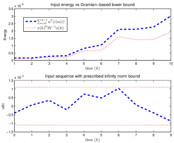
Figure 1: Input energy vs Gramian-based lower bound.

Figure 1 compares the input energy functional $\sum_{i=0}^{k-1}u^{2}(i)$ with the Gramian-based lower bound $x^{T}(k)\mathcal{W}^{-1}x(k)$ for $k\leq K=10$ and an arbitrarily chosen input sequence $\{u\}^{K-1}$ satisfying (42). Since the gap between the minimum input energy and the lower bound cannot be greater than the one shown in the plot, Figure 1 shows that the Gramian-based lower bound is a good estimate of the minimum input energy required to drive the state from the origin to another state. $\bullet$

V Reachability metrics for bilinear networks

The inequality (16) connecting the reachability Gramian and the minimum energy required to steer the system from the origin to an arbitrary terminal state allows us to extend the reachability metrics defined for complex linear systems in [7, 6, 8] to bilinear control systems. We therefore consider the minimum eigenvalue, the trace, and the determinant of the Gramian as reachability metrics. The minimum eigenvalue $\lambda_{\mathop{\mathrm{m}in}}(\mathcal{W})$ characterizes the minimum input energy required in the worst case to reach a state. Given the observation, cf. [8], that

$$\frac{\int_{\{x\in\mathbb{R}^{n}|\lVert x\lVert=1\}}x^{T}\mathcal{W}^{-1}xdx}{\int_{\{x\in\mathbb{R}^{n}|\lVert x\lVert=1\}}dx}=\frac{\mathop{\mathrm{t}r}(\mathcal{W}^{-1})}{n}\geq\frac{n}{\mathop{\mathrm{t}r}(\mathcal{W})},$$

the trace $\mathop{\mathrm{t}r}(\mathcal{W})$ characterizes the average minimum control energy required to reach a state. Finally, the determinant $\det(\mathcal{W})$ reflects the volume of the ellipsoid containing the reachable states using inputs with no more than unit energy.

Formally, our goal is to choose $m$ actuators from a given group of $M$ candidates ($m\leq M$) such that $\lambda_{\mathop{\mathrm{m}in}}(\mathcal{W})$, $\mathop{\mathrm{t}r}(\mathcal{W})$ or $\det(\mathcal{W})$ is maximized, depending on the specific objective at hand. Denoting $V=\{1,\dots,M\}$ and $S=\{s_{1},\dots,s_{m}\}$, we write this combinatorial optimization problem as

$$\max_{S\subseteq V}\;f(\mathcal{W}(S)),$$ (43)

where $f:\mathbb{R}^{n\times n}\rightarrow\mathbb{R}_{\geq 0}$ can be $\mathop{\mathrm{t}r}(\mathcal{\cdot})$, $\lambda_{\mathop{\mathrm{m}in}}(\mathcal{\cdot})$ or $\det(\mathcal{\cdot})$. We use $\mathcal{W}(S)$ instead of $\mathcal{W}$ to indicate its dependence on the choice of $S$. Similarly, we denote the input matrices $B$ and $F$ as $B_{S}=[b_{s_{1}}\hskip 4.30554pt\dots\hskip 4.30554ptb_{s_{m}}]$ and $F_{S}=[F_{s_{1}}\hskip 4.30554pt\dots\hskip 4.30554ptF_{s_{m}}]$, respectively, where $b_{i}\in\mathbb{R}^{n},F_{i}\in\mathbb{R}^{n\times n}$ for each $i\in V$. In general, the optimization problem (43) is NP-hard, as we justify below. The next result shows that the function mapping $S$ to $\mathcal{W}(S)$ displays the increasing returns property.

Theorem 3

(Increasing returns property of the function mapping $S$ to $\mathcal{W}(S)$). For any $S_{1}\subseteq S_{2}\subseteq V$ and $s\in V\backslash S_{2}$,

$$\mathcal{W}(S_{2}\cup\{s\})-\mathcal{W}(S_{2})\geq\mathcal{W}(S_{1}\cup\{s\})-\mathcal{W}(S_{1}).$$ (44)

Proof:

Without loss of generality, we relabel the elements in $V$ such that $S_{1}=\{1,\dots,m_{1}\}$, $S_{2}=\{1,\dots,m_{1}+m_{2}\}$ and $s=m_{1}+m_{2}+1$ with $m_{1}\geq 1$, $m_{2}\geq 0$ and $m_{1}+m_{2}+1\leq|V|=M$. For any $S=\{s_{1},\dots,s_{m}\}\subseteq V$, we have

$$\mathcal{W}_{1}(S) =\sum_{k=0}^{\infty}A^{k}B_{S}B_{S}^{T}(A^{T})^{k}$$

$$=\sum_{j=1}^{m}\sum_{k=0}^{\infty}A^{k}b_{s_{j}}b_{s_{j}}^{T}(A^{T})^{k}=\sum_{s\in S}\mathcal{W}_{1}(s),$$ (45)

which implies that

$$\mathcal{W}_{1}(S_{2}\cup\{s\})-\mathcal{W}_{1}(S_{2}) =\mathcal{W}_{1}(s)$$

$$=\mathcal{W}_{1}(S_{1}\cup\{s\})-\mathcal{W}_{1}(S_{1}).$$ (46)

For $i\geq 2$, using the last equation in (8) and cancelling terms in common, we obtain

$$\mathcal{W}_{i}(S_{2}\cup\{s\})-\mathcal{W}_{i}(S_{2})-\mathcal{W}_{i}(S_{1}\cup\{s\})+\mathcal{W}_{i}(S_{1})$$

$$\quad=\sum_{j_{1},j_{2}=1}^{m_{1}+m_{2}+1}\sum_{k=0}^{\infty}A^{k}F_{j_{2}}\mathcal{W}_{i-1}(s_{j_{1}})F_{j_{2}}^{T}(A^{T})^{k}$$

$$\quad\quad-\sum_{j_{1},j_{2}=1}^{m_{1}+m_{2}}\sum_{k=0}^{\infty}A^{k}F_{j_{2}}\mathcal{W}_{i-1}(s_{j_{1}})F_{j_{2}}^{T}(A^{T})^{k}$$

$$\quad\quad-\sum_{j_{1},j_{2}\in S_{1}\cup\{s\}}\sum_{k=0}^{\infty}A^{k}F_{j_{2}}\mathcal{W}_{i-1}(s_{j_{1}})F_{j_{2}}^{T}(A^{T})^{k}$$

$$\quad\quad+\sum_{j_{1},j_{2}=1}^{m_{1}}\sum_{k=0}^{\infty}A^{k}F_{j_{2}}\mathcal{W}_{i-1}(s_{j_{1}})F_{j_{2}}^{T}(A^{T})^{k}$$

$$\quad=\sum_{j=m_{1}+1}^{m_{2}}\sum_{k=0}^{\infty}A^{k}F_{m_{1}+m_{2}+1}\mathcal{W}_{i-1}(s_{j})F_{m_{1}+m_{2}+1}^{T}(A^{T})^{k}$$

$$\quad\quad+\sum_{j=m_{1}+1}^{m_{2}}\sum_{k=0}^{\infty}A^{k}F_{j}\mathcal{W}_{i-1}(s_{m_{1}+m_{2}+1})F_{j}^{T}(A^{T})^{k}$$

$$\quad\geq 0.$$

The proof then follows using the definition (4) of $\mathcal{W}$.    

Since the trace function is linear, Theorem 3 immediately implies that $\mathop{\mathrm{t}r}(\mathcal{W})$ is a supermodular function. For linear time-invariant systems, the inequality in (44) becomes an equality. This can be seen from the proof of Theorem 3 or found in [8]. Supermodularity in combinatorial optimization of functions over subsets is analogous to convexity in optimization of functions defined over Euclidean space. The maximization of supermodular functions under cardinality constraints is known to be NP-hard, but its Lagrangian dual and its continuous relaxation can be solved in polynomial time [37], which provides an upper bound on the optimal value. On the other hand, a lower bound on the optimal value follows from the following result.

Corollary 2

For any $S_{1}\subseteq S_{2}\subseteq V$ and $S_{3}\subseteq V\backslash S_{2}$,

$$\mathcal{W}(S_{2}\cup S_{3})-\mathcal{W}(S_{2})\geq\mathcal{W}(S_{1}\cup S_{3})-\mathcal{W}(S_{1}).$$ (47)

Proof:

Denote $S_{3}=\{s_{1},\dots,s_{\left|S_{3}\right|}\}$, it follows immediately from (44) that for any $i=1,\ldots,\left|S_{3}\right|$,

$$\mathcal{W}(S_{2}\cup\{s_{1},\dots,s_{i}\})-\mathcal{W}(S_{2}\cup\{s_{1},\dots,s_{i-1}\})$$

$$\geq\mathcal{W}(S_{1}\cup\{s_{1},\dots,s_{i}\})-\mathcal{W}(S_{1}\cup\{s_{1},\dots,s_{i-1}\}).$$ (48)

By summing inequality (48) with respect to $i=1,\ldots,\left|S_{3}\right|$, we obtain (47).    

Theorem 4

(Lower bound on reachability metrics). Let $f:\mathbb{R}^{n\times n}\rightarrow\mathbb{R}_{\geq 0}$ be either $\mathop{\mathrm{t}r}$, $\lambda_{\mathop{\mathrm{m}in}}$ or $\det$. Then for any set $S$ of $m$ actuators

$$f(\mathcal{W}(S))\geq\sum_{i=1}^{N}f(\mathcal{W}(S_{i})),$$ (49)

where $S_{1},\dots,S_{N}$ is any partition of $S$.

Proof:

By letting $S_{1}=\emptyset$ in (47) and using the fact that $\mathcal{W}(\emptyset)=\mathbf{0}_{n\times n}$, it holds immediately that for any subset $S\subseteq V$, $\mathcal{W}(S)\geq\sum_{i=1}^{N}\mathcal{W}(S_{i})$. This directly implies that $\mathop{\mathrm{t}r}(\mathcal{W}(S))\geq\sum_{i=1}^{N}\mathop{\mathrm{t}r}(\mathcal{W}(S_{i}))$. Moreover,

$$\lambda_{\mathop{\mathrm{m}in}}(\mathcal{W}(S)) =\min_{\lVert x\lVert=1}x^{T}\mathcal{W}(S)x$$

$$\geq\min_{\lVert x\lVert=1}x^{T}\bigl{(}\sum_{i=1}^{N}\mathcal{W}(S_{i})\bigr{)}x$$

$$\geq\sum_{i=1}^{N}\min_{\lVert x\lVert=1}x^{T}\mathcal{W}(S_{i})x=\sum_{i=1}^{N}\lambda_{\mathop{\mathrm{m}in}}(\mathcal{W}(S_{i})).$$

Finally, employing the Minkowski’s determinant inequality [38] (if $A$, $B\in\mathbb{R}^{n\times n}$ are positive definite matrices, then $\det(A+B)\geq\det(A)+\det(B)$) repeatedly, we obtain

$$\det(\mathcal{W}(S))\geq\sum_{i=1}^{N}\det(\mathcal{W}(S_{i}))$$

and the proof is complete.    

To maximize the lower bound in (49), one simply needs to compute $f(\mathcal{W}(s))$ individually for every $s\in V$, order the results in decreasing order, and select the actuators sequentially starting with the one with largest value. We refer to this procedure as the greedy algorithm. The following example illustrates its performance.

Example 3

(Controller selection via the greedy algorithm). Consider an augmented bilinear control system based on the model in Example 2,

$$x(k+1)=Ax(k)+\sum_{j\in S}(F_{j}x(k)+B_{j})u_{j}(k),$$

where $A$, $B_{0}=b$ and $F_{0}=f$ are the same as those given in (30). The other actuator candidates are $(F_{j},B_{j})$, where $B_{j}$ is the $j$-th canonical vector in $\mathbb{R}^{5}$ for $j\in\{1,2,3\}$. We let $F_{1}(1,2)=F_{1}(2,3)=0.02$, $F_{2}(2,5)=0.01$, $F_{2}(4,2)=0.05$, and $F_{3}(1,1)=0.05$, $F_{3}(4,5)=0.02$, with all the other elements in $F_{j}$ being zero, for $j\in\{1,2,3\}$. Table I shows their individual and combined contributions to $\lambda_{\mathop{\mathrm{m}in}}(\mathcal{W}(S))$, $\mathop{\mathrm{t}r}(\mathcal{W}(S))$, and $\det(\mathcal{W}(S))$.

TABLE I: Contribution of chosen sets of actuators to the Gramian-based reachability metrics.

$S$	$\mathop{\mathrm{t}r}(W(S))$	$\lambda_{\mathop{\mathrm{m}in}}(W(S))$	$\det(W(S))$	$S$	$\mathop{\mathrm{t}r}(W(S))$	$\lambda_{\mathop{\mathrm{m}in}}(W(S))$	$\det(W(S))$
$\{0\}$	$14.42$	$0.027$	$0.242$	$\{0,2\}$	$19.91$	$0.07$	$3.32$
$\{1\}$	$5.03$	$0.023$	$0.025$	$\{0,3\}$	$18.69$	$0.05$	$1.13$
$\{2\}$	$4.04$	$3\times 10^{-5}$	$9\times 10^{-7}$	$\{0,1,2\}$	$26.50$	$0.137$	$46.15$
$\{3\}$	$3.03$	$1.6\times 10^{-6}$	$4\times 10^{-11}$	$\{0,1,3\}$	$25.28$	$0.125$	$28.68$
$\{0,1\}$	$20.98$	$0.09$	$11.704$	$\{0,2,3\}$	$24.19$	$0.103$	$8.34$

We make the following observations:

1. Actuators with a large individual contribution provide a large combinatorial contribution. This fact suggests that the greedy algorithm is a sensible strategy, even though $\sum_{s\in S}f(\mathcal{W}(s))$ can be considerably smaller than $f(\mathcal{W}(S))$ for $f=\lambda_{\mathop{\mathrm{m}in}}$ and $\det$.

2. For $f=\mathop{\mathrm{t}r}$, $\sum_{s\in S}\mathop{\mathrm{t}r}(\mathcal{W}(s))$ is a good estimate of $\mathop{\mathrm{t}r}(\mathcal{W}(S))$. For example,

   $$\frac{\mathop{\mathrm{t}r}(\mathcal{W}(\{0,1\}))-\sum_{s\in\{0,1\}}\mathop{\mathrm{t}r}(\mathcal{W}(s))}{\mathop{\mathrm{t}r}(\mathcal{W}(\{0,1\}))}$$

   $$\quad=\frac{20.98-14.42-5.03}{20.98}=0.073,$$

   i.e., a relative error less than $8\%$.

As an example, for the case $m=2$, the greedy algorithm will select $\{0,1\}$, which is the optimal choice. We have observed similar results for various simulations of this example with several sets of randomly generated $(B_{j},F_{j})$. $\bullet$

VI Addition of bilinear inputs to linear symmetric networks

In this section, we examine the effect that the addition of bilinear inputs has on the worst-case minimum input energy for difficult-to-control linear networks. We begin by formalizing this notion.

Definition 2

(Difficult-to-control networks). A class of networks is said to be difficult to control (DTC) if, for a fixed number of control inputs, the normalized worst-case minimum energy grows unbounded with the scale of the network, i.e.,

$$\lim_{n\rightarrow\infty}\sup_{x_{f}\in\mathbb{R}^{n}}\inf_{\begin{subarray}{c}\{u\}^{\infty}:u(k)\in\mathbb{R}^{m},\\ x(\infty)=x_{f}\end{subarray}}\frac{\lVert\{u\}^{\infty}\rVert^{2}}{\lVert x_{f}\rVert^{2}}\rightarrow\infty,$$

where $x(\infty)\triangleq\lim_{k\rightarrow\infty}x(k)$.

For linear networks $(A(n),\mathbf{0}_{n\times nm},B(n))$, one can see from (14) that

$$\sup_{x_{f}\in\mathbb{R}^{n}:\lVert x_{f}\rVert^{2}=1}\inf_{\begin{subarray}{c}\{u\}^{\infty}:u(k)\in\mathbb{R}^{m},\\ x(\infty)=x_{f}\end{subarray}}\lVert\{u\}^{\infty}\rVert^{2}=\lambda_{\min}^{-1}(\mathcal{W}_{1}(n)).$$

Therefore, if the linear network is difficult to control, this implies that the minimum eigenvalue of the reachability Gramian approaches $0$ as $n$ grows. A typical class of difficult-to-control linear networks is the class of stable and symmetric networks for which, cf. [7, Corollary 3.2], the worst-case minimum input energy grows exponentially with rate $\frac{n}{m}$ for any choice of $B(n)\in\mathbb{R}^{n\times m}$ whose columns are canonical vectors in $\mathbb{R}^{n}$ (here, $m$ is the number of control inputs or control nodes).

Our first result of this section shows that difficult-to-control linear symmetric networks remain so after the addition of a finite number of bilinear inputs.

Theorem 5

(Difficult-to-control linear symmetric networks remain so after granted the ability to control a finite number of interconnections). Consider a class of difficult-to-control linear symmetric networks $(A(n),\mathbf{0}_{n\times nm},B(n))$. The class of bilinear networks $(A(n),F(n),B(n))$ is also DTC if the number of nonzero entries in the matrix $F(n)\in\mathbb{R}^{n\times nm}$ and $\rVert F(n)\rVert_{\max}\triangleq\max_{i,j}\left|F_{ij}(n)\right|$ are uniformly bounded with respect to $n$.

Proof:

Our proof has two parts. First, we construct a class of bilinear control system whose trajectories include the trajectories of the systems $(A(n),F(n),B(n))$. Second, we establish a correspondence between the constructed bilinear systems and linear control networks, and build on it to show that they are difficult to control. For the first step, let $\lvert\cdot\rvert_{nz}$ denote the number of nonzero entries in a matrix and define $M_{F}=\sum_{j=1}^{m}\lvert F_{j}(n)\rvert_{nz}$. Select matrices $\hat{F}_{j}(n)$ with $\rvert\hat{F}_{j}(n)\rvert_{nz}=1$ for $j\in\{1,\dots,M_{F}\}$ and

$$\sum_{j=\lvert F_{i-1}(n)\rvert_{nz}+1}^{\lvert F_{i}(n)\rvert_{nz}}\hat{F}_{j}(n)=F_{i}(n),$$

for $i\in\{1,\dots,m\}$, where $\lvert F_{0}(n)\rvert_{nz}\triangleq 0$ for convenience. Consider the bilinear system

$$x(k+1)=A(n)x(k)+\sum_{j=1}^{M_{F}}\hat{F}_{j}(n)x(k)v_{j}(k)+\sum_{j=1}^{m}B_{j}(n)u_{j}(k),$$ (50)

with state $x(k)\in\mathbb{R}^{n}$, inputs $u_{j}(k),v_{j}(k)\in\mathbb{R}$, and system matrices $A(n),\hat{F}_{j}(n)\in\mathbb{R}^{n\times n}$, $B_{j}(n)\in\mathbb{R}^{n}$. Note that, selecting $v_{j}(k)=u_{i}(k)$ for $j=\lvert F_{i-1}(n)\rvert_{nz}+1,\ldots,\lvert F_{i}(n)\rvert_{nz}$ and $i\in\{1,\dots,m\}$ makes (50) take the form

$$x(k+1)=A(n)x(k)+\sum_{j=1}^{m}(F_{j}(n)x(k)+B_{j}(n))u_{j}(k),$$

which corresponds to the bilinear network $(A(n),F(n),B(n))$. This implies that the optimal control sequence $\{u^{\ast}\}^{\infty}$ for $(A(n),F(n),B(n))$ generates the same network state trajectory as the (not necessarily optimal) control sequence $\{v^{\ast},u^{\ast}\}^{\infty}$ for (50).

Our second step establishes that the bilinear network in (50) is difficult to control. Assume that the nonzero entry in $\hat{F}_{j}(n)$ is in the $i$-th row. Then, there exist $M_{F}$ scalar sequences $\{\hat{u}_{j}(k)\}$ such that for all $j\in\{1,\dots,M_{F}\}$ and all $k\in\mathbb{Z}_{\geq 0}$,

$$\hat{F}_{j}(n)x(k)v_{j}(k)=\hat{B}_{j}\hat{u}_{j}(k),$$ (51)

where $\hat{B}_{j}=e_{i}$ is the $i$-th canonical unit vector in $\mathbb{R}^{n}$. Substituting this into (50), we obtain

$$x(k+1)=A(n)x(k)+\sum_{j=1}^{M_{F}}\hat{B}_{j}\hat{u}_{j}(k)+\sum_{j=1}^{m}B_{j}(n)u_{j}(k),$$ (52)

which is linear, symmetric and difficult to control because its number of control nodes is at most $m+M_{F}$, which is constant. Furthermore, there exists a constant $\bar{X}\in\mathbb{R}_{>0}$, such that for all $i=1,\ldots,n$, and all $k\in\mathbb{Z}_{\geq 0}$, $\rVert x_{i}(k)\rVert\leq\bar{X}$ since the state trajectory starts at the origin, the network is stable and the input is bounded. As a result,

$$\sup_{x_{f}\in\mathbb{R}^{n}}\inf_{\underset{\text{equation (\ref{eq1:Pf_Theo6})}}{\{u,v\}^{\infty}}}\lVert\{u,v\}^{\infty}\rVert^{2}\lVert x_{f}\rVert^{-2}$$

$$\quad\overset{\text{(\ref{eq3:Pf_Theo6})}}{\geq}\sup_{x_{f}\in\mathbb{R}^{n}:\lVert x_{f}\rVert^{2}=1}\inf_{\underset{\text{equation (\ref{eq4:Pf_Theo6})}}{\{u,\hat{u}\}^{\infty}}}(\lVert\{u\}^{\infty}\rVert^{2}+\rVert F\rVert_{\max}^{-2}\bar{X}^{-2}\lVert\{\hat{u}\}^{\infty}\rVert^{2})$$

$$\quad\geq\min(1,\rVert F\rVert_{\max}^{-2}\bar{X}^{-2})$$

$$\quad\quad\cdot\sup_{x_{f}\in\mathbb{R}^{n}:\lVert x_{f}\rVert^{2}=1}\inf_{\underset{\text{equation (\ref{eq4:Pf_Theo6})}}{\{u,\hat{u}\}^{\infty}}}(\lVert\{u\}^{\infty}\rVert^{2}+\lVert\{\hat{u}\}^{\infty}\rVert^{2}),$$

which implies the result.    

Our next result shows that difficult-to-control linear symmetric networks might remain so even after relaxing the finiteness of the number of interconnections that can be affected by the addition of bilinear inputs. More concretely, we study the reachability properties of the class of networks $(A,F,B)$ with symmetric adjacency matrices $A=A^{T}$ and $F=\alpha I_{n}$, $|\mathop{\mathrm{t}r}(F)|\leq\mu(n)\in o(\sqrt{n})$ (without loss of generality, we let $\alpha\geq 0$). For instance, this corresponds to the case when a central controller can affect the strengths of the self-loops of all agents simultaneously in a linear symmetric network or when all agents simultaneously adjust the strength of their self-loops by the same amount.

Theorem 6

(Worst-case control energy for linear symmetric networks with self-loop modulation). Consider the class of bilinear networks given by

$$x(k+1)=(A+\alpha v(k)I_{n})x(k)+\sum_{j=1}^{m}B_{j}u_{j}(k),$$

with $A=A^{T}$, $|\mathop{\mathrm{t}r}(\alpha I_{n})|\leq\mu(n)\in o(\sqrt{n})$ and $\rho(A)<\sqrt{1-T_{m}^{-1}}$, where $T_{m}\triangleq\left\lceil\frac{n}{m}\right\rceil-1$. Then the reachability Gramian of the network satisfies, for any $n>m^{-1}\mu^{2}(n)$,

$$\lambda_{\min}(\mathcal{W})\leq\frac{(1-T_{m}\alpha^{2})^{-1}}{1-\rho^{2}(A)-T_{m}^{-1}}\rho^{2T_{m}}(A).$$ (53)

Proof:

Define $\mathop{\mathrm{s}um}(k,i)\triangleq k_{1}+\dots+k_{i}$ for $k\in\{\mathbb{Z}_{\geq 0}\}^{\infty}$ and $i\in\mathbb{Z}_{\geq 1}$. By definition of the reachability Gramian (4), it follows that

$$\mathcal{W}_{i} =\alpha^{2(i-1)}\sum_{k_{1},\dots,k_{i}=0}^{\infty}A^{\mathop{\mathrm{s}um}(k,i)}BB^{T}(A^{T})^{\mathop{\mathrm{s}um}(k,i)}$$

$$=\mathcal{W}_{i,s}+\mathcal{W}_{i,f},$$

where

$$\mathcal{W}_{i,s} \triangleq\alpha^{2(i-1)}\sum_{k_{1},\dots,k_{i}=0}^{\mathop{\mathrm{s}um}(k,i)<T_{m}}A^{\mathop{\mathrm{s}um}(k,i)}BB^{T}(A^{T})^{\mathop{\mathrm{s}um}(k,i)},$$

$$\mathcal{W}_{i,f} \triangleq\alpha^{2(i-1)}\sum_{k_{1},\dots,k_{i}=0}^{\mathop{\mathrm{s}um}(k,i)\geq T_{m}}A^{\mathop{\mathrm{s}um}(k,i)}BB^{T}(A^{T})^{\mathop{\mathrm{s}um}(k,i)}.$$

Therefore,

$$\lambda_{\min}(\mathcal{W}) =\lambda_{\min}\big{(}\sum_{i=1}^{\infty}\mathcal{W}_{i,s}+\sum_{i=1}^{\infty}\mathcal{W}_{i,f}\big{)}$$ (54)

$$\leq\lambda_{\min}\big{(}\sum_{i=1}^{\infty}\mathcal{W}_{i,s}\big{)}+\sum_{i=1}^{\infty}\lVert\mathcal{W}_{i,f}\rVert\leq\sum_{i=1}^{\infty}\lVert\mathcal{W}_{i,f}\rVert,$$

where the first inequality follows from the Bauer-Fike theorem [38] and the second inequality follows by noting that $\sum_{i=1}^{\infty}\mathcal{W}_{i,s}$ is singular because its column space is contained in the space spanned by $\{B,AB,\dots,A^{T_{m}-1}B\}$, whose dimension is smaller than $n$ by definition of $T_{m}$. We can write $\mathcal{W}_{i,f}$ in a recursive manner as follows,

$$\mathcal{W}_{i,f} =\alpha^{2(i-1)}\sum_{k_{i}=0}^{\infty}A^{k_{i}}\bigl{(}\sum_{k_{1},\dots,k_{i-1}=0}^{\mathop{\mathrm{s}um}(k,i-1)\geq T_{m}}A^{\mathop{\mathrm{s}um}(k,i-1)}B$$

$$\quad\quad\cdot B^{T}(A^{T})^{\mathop{\mathrm{s}um}(k,i-1)}\bigr{)}(A^{T})^{k_{i}}$$

$$\quad+\alpha^{2(i-1)}\sum_{j=0}^{T_{m}-1}\sum_{k_{i}=T_{m}-j}^{\infty}\bigl{(}\sum_{k_{1},\dots,k_{i-1}=0}^{\mathop{\mathrm{s}um}(k,i-1)=j}A^{\mathop{\mathrm{s}um}(k,i)}B$$

$$\quad\quad\cdot B^{T}(A^{T})^{\mathop{\mathrm{s}um}(k,i)}\bigr{)}$$

$$=\alpha^{2}\sum_{k_{i}=0}^{\infty}A^{k_{i}}\mathcal{W}_{i-1,f}(A^{T})^{k_{i}}$$

$$\quad+\alpha^{2(i-1)}\displaystyle\sum_{j=0}^{T_{m}-1}\mathcal{\eta}(i-1,j)\mathcal{W}_{1,f},$$

where $\mathcal{\eta}(N,M)$ is the number of ways of choosing $N\in\mathbb{Z}_{\geq 0}$ non-negative integers such that their sum equals $M\in\mathbb{Z}_{\geq 0}$. Two properties of this function are useful to us: (i) $\mathcal{\eta}(N,M)=\sum_{j=0}^{M}\mathcal{\eta}(N-1,j)$ and (ii) $\mathcal{\eta}(N,M)$ is an increasing function of $N$ and $M$. Using (i), we obtain

$$\mathcal{W}_{i,f}=\alpha^{2}\!\displaystyle\sum_{k_{i}=0}^{\infty}A^{k_{i}}\mathcal{W}_{i-1,f}(A^{T})^{k_{i}}\!+\!\alpha^{2(i-1)}\mathcal{\eta}(i,T_{m}-1)\mathcal{W}_{1,f}.$$

Taking norms and upper bounding, we get

$$\lVert\mathcal{W}_{i,f}\rVert \leq\frac{\alpha^{2}}{1-\lVert A\rVert^{2}}\lVert\mathcal{W}_{i-1,f}\rVert+\alpha^{2(i-1)}\mathcal{\eta}(i,T_{m}-1)\lVert\mathcal{W}_{1,f}\rVert.$$

Using this inequality repeatedly, we obtain

$$\lVert\mathcal{W}_{i,f}\rVert \leq\sum_{j=0}^{i-1}\frac{\alpha^{2(i-1)}}{(1-\lVert A\rVert^{2})^{j}}\mathcal{\eta}(i-j,T_{m}-1)\lVert\mathcal{W}_{1,f}\rVert$$

$$\leq(T_{m}\alpha^{2})^{(i-1)}\lVert\mathcal{W}_{1,f}\rVert\sum_{j=0}^{i-1}T_{m}^{-j}(1-\lVert A\rVert^{2})^{-j}$$

where we have used $\mathcal{\eta}(N,M)\leq(M+1)\mathcal{\eta}(N-1,M)\leq(M+1)^{N-1}\mathcal{\eta}(1,M)=(M+1)^{N-1}$, which follows from properties (i) and (ii) of $\eta$ above. Since $A$ is symmetric and Schur stable, $\lVert A\rVert=\rho(A)$, which together with $\rho(A)<\sqrt{1-T_{m}^{-1}}$ implies $T_{m}^{-1}(1-\lVert A\rVert^{2})^{-1}<1$. Therefore, we conclude

$$\lVert\mathcal{W}_{i,f}\rVert \leq\frac{(T_{m}\alpha^{2})^{(i-1)}\lVert\mathcal{W}_{1,f}\rVert}{1-T_{m}^{-1}(1-\lVert A\rVert^{2})^{-1}}.$$ (55)

Combining (54) with (55), we obtain

$$\lambda_{\min}(\mathcal{W}) \leq\sum_{i=1}^{\infty}\frac{(T_{m}\alpha^{2})^{(i-1)}\lVert\mathcal{W}_{1,f}\rVert}{1-T_{m}^{-1}(1-\rho^{2}(A))^{-1}}$$

$$=\frac{(1-T_{m}\alpha^{2})^{-1}}{1-T_{m}^{-1}(1-\rho^{2}(A))^{-1}}\lVert\mathcal{W}_{1,f}\rVert,$$

where we have used the fact that $|\mathop{\mathrm{t}r}(F)|\leq\mu(n)$ implies that $T_{m}\alpha^{2}<1$ for $n>m^{-1}\mu^{2}(n)$. Using [7, Theorem 3.1], we obtain

$$\lambda_{\min}(\mathcal{W}) \leq\frac{(1-T_{m}\alpha^{2})^{-1}}{1-T_{m}^{-1}(1-\rho^{2}(A))^{-1}}\frac{\rho^{2T_{m}}(A)}{1-\rho^{2}(A)}$$

$$=\frac{(1-T_{m}\alpha^{2})^{-1}}{1-\rho^{2}(A)-T_{m}^{-1}}\rho^{2T_{m}}(A),$$

and the proof is complete.    

Note that, for a large-scale network with a fixed number of control nodes, the assumption that $\rho(A)<\sqrt{1-T_{m}^{-1}}$ in Theorem 6 is not restrictive because $\sqrt{1-T_{m}^{-1}}$ becomes arbitrarily close to $1$ as $n$ increases. One can show that $\frac{(1-T_{m}\alpha^{2})^{-1}}{1-\rho^{2}(A)-T_{m}^{-1}}$ in (53) is a decreasing function of $n$ and that

$$\lim_{n\rightarrow\infty}\frac{(1-T_{m}\alpha^{2})^{-1}}{1-\rho^{2}(A)-T_{m}^{-1}}=(1-\rho^{2}(A))^{-1}.$$

Thus, $\lambda_{\min}(\mathcal{W})$ decreases at least exponentially as $n$ increases, which means the worst-case control energy increases exponentially, as indicated by Theorem 2. Therefore Theorem 6 can be interpreted as saying that bounded homogeneous self-loop modulation through bilinear inputs does not make a linear symmetric network easier to control.

We illustrate the result in Theorem 6 with an example.

Example 4

(Line network with self-loop modulation). Consider the group of line networks for $n\in\{1,\dots,15\}$ with adjacency matrices $A=[a_{ij}]$, where $a_{ij}=0.25$ if $|i-j|\leq 1$ and $a_{ij}=0$ otherwise for $i,j\in{\{1,\dots,n\}}$. Let $m=3$, with $B_{1},B_{2},B_{3}$ being canonical vectors chosen optimally using exhaustive search to maximize $\lambda_{\min}(\mathcal{W})$, and let $|\mathop{\mathrm{t}r}(\alpha I_{n})|=0.9$. The minimum eigenvalue of the reachability Gramian is plotted in a logarithmic scale in Figure 2 as a function of $n$. It can be seen that $\lambda_{\min}(\mathcal{W})$ decreases exponentially as $n$ increases, which implies that the worst-case control energy increases exponentially with the scale of the network, even with self-loop modulation.

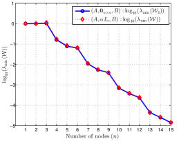
Figure 2: For the class of line networks described in Example 4, $\log_{10}(\lambda_{\min}(\mathcal{W}))$ is plotted in red diamonds as the scale $n$ of the network increases from $1$ to $15$. The same quantity is also plotted in blue circles for the case without self-loop modulation ($F=\mathbf{0}_{n\times n}$). As predicted by Theorem 6, symmetric networks with or without self-loop modulation are difficult to control with a fixed number of control nodes.

$\bullet$

We conclude this section with an example that shows that a difficult-to-control linear network can be made easy to control by adding a single bilinear input that affects an infinite number of interconnections with strength that is independent of the scale of the network.

Example 5

(Linear symmetric line network with $n$-dependent interconnection modulation). Consider the group of bilinear networks $(A(n),F(n),B(n))$ with

$$A(n) = \left[\begin{array}[]{ccccc}0.05&0.05&0&\dots&0\\ 0.05&0.05&0.05&\ddots&\vdots\\ 0&0.05&\ddots&\ddots&0\\ \vdots&\ddots&\ddots&\ddots&0.05\\ 0&\dots&0&0.05&0.05\end{array}\right]\in\mathbb{R}^{n\times n},$$

$$B(n) = \left[\begin{array}[]{cccc}1&0&\dots&0\end{array}\right]^{T}\in\mathbb{R}^{n},$$

and $F(n)=[f_{ij}]$ with $f_{ij}=1$ if $i=j+1$ and all the other entries $0$. Figure 3 compares $\lambda_{\min}(\mathcal{W}_{1}\mathcal{)}$ of the linear line network $(A(n),\mathbf{0}_{n\times nm},B(n))$ with $\lambda_{\min}(\mathcal{W})$ of the bilinear network $(A(n),F(n),B(n))$. One can see that $\lambda_{\min}(\mathcal{W}_{1}\mathcal{)}$ decreases exponentially as the scale $n$ of the network increases, which implies that the linear network is difficult to control. By employing the bilinear control through $F(n)$, $\lambda_{\min}(\mathcal{W)}$ is kept constant as $n$ increases. Note that the number of interconnections we need to modulate increases with $n$.

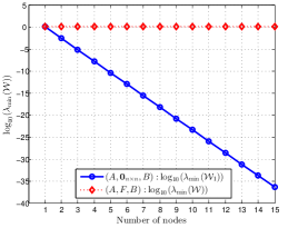
Figure 3: The class of linear networks $(A,\mathbf{0}_{n\times nm},B)$ are difficult to control while the corresponding bilinear networks $(A,F,B)$ are easy to control.

$\bullet$

VII Conclusions

We have proposed Gramian-based reachability metrics for discrete-time bilinear control networks to quantify the input energy required to steer the state from the origin to an arbitrary point. Our reachability notions build on the fact that, when the infinity norm of the input is upper bounded by some function of the system matrices, then the required minimum input energy can be lower bounded in terms of the reachability Gramian. We have studied the supermodularity properties of Gramian as a function of the actuators and derived lower bounds on the reachability metrics in terms of the aggregate contribution of the individual actuators. Finally, we have studied the effect that the addition of bilinear inputs has on the difficult-to-control character of linear symmetric networks. Future work will include the design of algorithms for optimal selection of control nodes in complex networks, where both the nodes and the interconnection strength among neighboring nodes can be affected by actuators, the study of the more general problem of steering the network state from an arbitrary initial condition to an arbitrary target state, and the analysis of observability metrics for bilinear control systems based on the generalized observability Gramian.

References

• [1] Y. Zhao and J. Cortés, “Reachability metrics for bilinear complex networks,” in IEEE Conf. on Decision and Control, Osaka, Japan, 2015, pp. 4788–4793.
• [2] Y. Y. Liu, J. J. Slotine, and A. L. Barabási, “Controllability of complex networks,” Nature, vol. 473, no. 7346, pp. 167–173, 2011.
• [3] A. Olshevsky, “Minimal controllability problems,” IEEE Transactions on Control of Network Systems, vol. 1, no. 4, pp. 249–258, 2014.
• [4] A. Rahmani, M. Ji, M. Mesbahi, and M. Egerstedt, “Controllability of multi-agent systems from a graph-theoretic perspective,” SIAM Journal on Control and Optimization, vol. 48, no. 1, pp. 162–186, 2009.
• [5] C. Aguilar and B. Gharesifard, “Necessary conditions for controllability of nonlinear networked control systems,” in American Control Conference, Portland, OR, USA, 2014, pp. 5379–5383.
• [6] G. Yan, J. Ren, Y. Lai, C. Lai, and B. Li, “Controlling complex networks: How much energy is needed?” Physical Review Letters, vol. 108, no. 21, p. 218703, 2012.
• [7] F. Pasqualetti, S. Zampieri, and F. Bullo, “Controllability metrics, limitations and algorithms for complex networks,” IEEE Transactions on Control of Network Systems, vol. 1, no. 1, pp. 40–52, 2014.
• [8] T. Summers and J. Lygeros, “Optimal sensor and actuator placement in complex dynamical networks,” in World Congress, vol. 19, no. 1, 2014, pp. 3784–3789.
• [9] V. Tzoumas, M. A. Rahimian, G. J. Pappas, and A. Jadbabaie, “Minimal actuator placement with optimal control constraints,” arXiv preprint arXiv:1503.04693, 2015.
• [10] K. J. Friston, L. Harrison, and W. Penny, “Dynamic causal modelling,” NeuroImage, vol. 19, pp. 1273–1302, 2003.
• [11] J. R. Iversen, A. Ojeda, T. Mullen, M. Plank, J. Snider, G. Cauwenberghs, and H. Poizner, “Causal analysis of cortical networks involved in reaching to spatial targets,” in Annual Int. Conf. of the IEEE Engineering in Medicine and Biology Society, Chicago, IL, 2014, pp. 4399–4402.
• [12] C. Bruni, G. Dipillo, and G. Koch, “Bilinear systems: An appealing class of "nearly linear" systems in theory and applications,” IEEE Transactions on Automatic Control, vol. 19, no. 4, pp. 334–348, 1974.
• [13] D. Elliott, Bilinear Control Systems: Matrices in Action.   Springer Science & Business Media, 2009, vol. 169.
• [14] P. Pardalos and V. Yatsenko, Optimization and Control of Bilinear Systems: Theory, Algorithms, and Applications.   Springer Science & Business Media, 2010, vol. 11.
• [15] D. Koditschek and K. Narendra, “The controllability of planar bilinear systems,” IEEE Transactions on Automatic Control, vol. 30, no. 1, pp. 87–89, 1985.
• [16] U. Piechottka and P. Frank, “Controllability of bilinear systems,” Automatica, vol. 28, no. 5, pp. 1043–1045, 1992.
• [17] T. Goka, T. Tarn, and J. Zaborszky, “On the controllability of a class of discrete bilinear systems,” Automatica, vol. 9, no. 5, pp. 615–622, 1973.
• [18] L. Tie and K. Cai, “On near-controllability and stabilizability of a class of discrete-time bilinear systems,” Systems & Control Letters, vol. 60, no. 8, pp. 650–657, 2011.
• [19] W. Gray and J. Mesko, “Energy functions and algebraic Gramians for bilinear systems,” in Preprints of the 4th IFAC Nonlinear Control Systems Design Symposium, 1998, pp. 103–108.
• [20] E. Verriest, “Time variant balancing and nonlinear balanced realizations,” in Model Order Reduction: Theory, Research Aspects and Applications, 2008, pp. 213–250.
• [21] P. Benner and T. Damm, “Lyapunov equations, energy functionals, and model order reduction of bilinear and stochastic systems,” SIAM Journal on Control and Optimization, vol. 49, no. 2, pp. 686–711, 2011.
• [22] L. Zhang, J. Lam, B. Huang, and G. Yang, “On Gramians and balanced truncation of discrete-time bilinear systems,” International Journal of Control, vol. 76, no. 4, pp. 414–427, 2003.
• [23] S. AL-Baiyat, M. Bettayeb, and U. AL-Saggaf, “New model reduction scheme for bilinear systems,” International Journal of Systems Science, vol. 25, no. 10, pp. 1631–1642, 1994.
• [24] W. Gray and E. Verriest, “Algebraically defined Gramians for nonlinear systems,” in 45th IEEE Conference on Decision and Control, 2006, pp. 3730–3735.
• [25] L. Zhang and J. Lam, “On ${H}_{2}$ model reduction of bilinear systems,” Automatica, vol. 38, no. 2, pp. 205–216, 2002.
• [26] P. Benner, T. Breiten, and T. Damm, “Generalised tangential interpolation for model reduction of discrete-time MIMO bilinear systems,” International Journal of Control, vol. 84, no. 8, pp. 1398–1407, 2011.
• [27] M. Petreczky, R. Wisniewski, and J. Leth, “Balanced truncation for linear switched systems,” Nonlinear Analysis: Hybrid Systems, vol. 10, pp. 4–20, 2013.
• [28] T. Kailath, Linear Systems.   Englewood Cliffs, New Jersey: Prentice-Hall, 1980.
• [29] R. G. Agniel and E. I. Jury, “Almost sure boundedness of randomly sampled systems,” SIAM Journal on Control, vol. 9, no. 3, pp. 372–384, 1971.
• [30] A. Hotz and R. E. Skelton, “Covariance control theory,” International Journal of Control, vol. 46, no. 1, pp. 13–32, 1987.
• [31] R. E. Skelton, S. M. Kherat, and E. Yaz, “Covariance control of discrete stochastic bilinear systems,” in American Control Conference, Boston, MA, USA, 1991, pp. 2660–2664.
• [32] Z. Aganovic and Z. Gajic, “The successive approximation procedure for finite-time optimal control of bilinear systems,” IEEE Transactions on Automatic Control, vol. 39, no. 9, pp. 1932–1935, 1994.
• [33] G. Y. Tang, H. Ma, and B. L. Zhang, “Successive-approximation approach of optimal control for bilinear discrete-time systems,” in IEE Proceedings-Control Theory and Applications, vol. 152, no. 6, 2005, pp. 639–644.
• [34] E. Hofer and B. Tibken, “An iterative method for the finite-time bilinear-quadratic control problem,” Journal of Optimization Theory and Applications, vol. 57, no. 3, pp. 411–427, 1988.
• [35] S. Boyd and L. Vandenberghe, Convex Optimization.   Cambridge University Press, 2009.
• [36] T. Hinamoto and S. Maekawa, “Approximation of polynomial state-affine discrete-time systems,” IEEE Transactions on Circuits and Systems, vol. 31, no. 8, pp. 713–721, 1984.
• [37] G. Gallo and B. Simeone, “On the supermodular knapsack problem,” Mathematical Programming, vol. 45, no. 1-3, pp. 295–309, 1989.
• [38] R. A. Horn and C. R. Johnson, Matrix Analysis.   Cambridge University Press, 1985.