Estimating the Division Kernel of a Size-Structured Population

Van Ha Hoang 111Laboratoire Paul Painlevé UMR CNRS 8524, Université Lille 1.
     Email address: van-ha.hoang@math.univ-lille1.fr
Abstract

We consider a size-structured population describing the cell divisions. The cell population is described by an empirical measure and we observe the divisions in the continuous time interval [0,T]0𝑇[0,T]. We address here the problem of estimating the division kernel hh (or fragmentation kernel) in case of complete data. An adaptive estimator of hh is constructed based on a kernel function K𝐾K with a fully data-driven bandwidth selection method. We obtain an oracle inequality and an exponential convergence rate, for which optimality is considered.

Keywords: random size-structured population, division kernel, nonparametric estimation, Goldenshluger-Lepski’s method, adaptive estimator, penalization, optimal rate.

1 Introduction

Models for populations of dividing cells possibly differentiated by covariates such as size have made the subject of an abundant literature in recent years (starting from Athreya and Ney [3], Harris [18], Jagers [28]…) Covariates termed as ‘size’ are variables that grow deterministically with time (such as volume, length, level of certain proteins, DNA content, etc.) Such models of structured populations provide descriptions for the evolution of the size distribution, which can be interesting for applications. For instance, in the spirit of Stewart et al. [33], we can imagine that each cell contains some toxicities whose quantity plays the role of the size. The asymmetric divisions of the cells, where one daughter contains more toxicity than the other, can lead under some conditions to the purge of the toxicity in the population by concentrating it into few lineages. These results are linked with the concept of aging for cell lineage. This concept has been tackled in many papers (e.g. Ackermann et al. [2], Aguilaniu et al. [1], C-Y. Lai et al. [22], Evans and Steinsaltz [15], Moseley [27]…).

Here we consider a stochastic individual-based model of size-structured population in continuous time, where individuals are cells undergoing asymmetric binary divisions and whose size is the quantity of toxicity they contain. A cell containing a toxicity x+𝑥subscriptx\in\mathbb{R}_{+} divides at a rate R>0𝑅0R>0. The toxicity grows inside the cell with rate α>0𝛼0\alpha>0. When a cell divides, a random fraction Γ[0,1]Γ01\Gamma\in[0,1] of the toxicity goes in the first daughter cell and 1Γ1Γ1-\Gamma in the second one. If Γ=12Γ12\Gamma=\frac{1}{2}, the daughters are the same with toxicity x2𝑥2\frac{x}{2}. We assume that ΓΓ\Gamma has a symmetric distribution on [0,1]01[0,1] with a density hh with respect to Lebesgue measure such that (Γ=0)=(Γ=1)=0Γ0Γ10\mathbb{P}(\Gamma=0)=\mathbb{P}(\Gamma=1)=0. If hh is piked at 1/2121/2 (i.e. Γ1/2similar-to-or-equalsΓ12\Gamma\simeq 1/2), then both daughters contain the same toxicity, i.e. the half of their mother’s toxicity. The more hh puts weight in the neighbourhood of 00 and 111, the more asymmetric the divisions are, with one daughter having little toxicity and the other a toxicity close to its mother’s one. If we consider that having a lot of toxicity is a kind of senescence, then, the kurtosis of hh provides indication on aging phenomena (see [24]).

Modifications of this model to account for more complex phenomena have been considered in other papers. Bansaye and Tran [6], Cloez [11] or Tran [35] consider non-constant division and growth rates. Robert et al. [29] studies whether divisions can occur only when a size threshold is reached. Our purpose here is to estimate the density hh ruling the divisions, and we stick to constant rates R𝑅R and α𝛼\alpha for the sake of simplicity. Notice that several similar models for binary cell division in discrete time also exist in the literature and have motivated statistical question as here, see for instance Bansaye et al. [4, 7], Bercu et al. [8], Bitseki Penda [10], Delmas and Marsalle [12] or Guyon [17].

Refer to caption
Figure 1: Trajectories of two daughter cells after a division, separating after the first division at time t1subscript𝑡1t_{1}.

Individual-based models provide a natural framework for statistical estimation. Estimation of the division rate is, for instance, the subject of Doumic et al. [13, 14] and Hoffmann and Olivier [19]. Here, the density hh is the kernel division that we want to estimate. Assuming that we observe the divisions of cells in continuous time on the interval [0,T]0𝑇[0,T], with T>0𝑇0T>0, we propose an adaptive kernel estimator h^^\hat{h} of hh for which we obtain an oracle inequality in Theorem 2. The construction of h^^\hat{h} is detailed in the sequel. From oracle inequality we can infer adaptive exponential rates of convergence with respect to T𝑇T depending on β𝛽\beta the smoothness of the density. Most of the time, nonparametric rates are of the form n2β2β+1superscript𝑛2𝛽2𝛽1n^{-\frac{2\beta}{2\beta+1}} (see for instance Tsybakov [36]) and exponential rates are not often encountered in the literature. The exponential rates are due to binary splitting, the number of cells i.e the sample size increases exponentially in exp(RT)𝑅𝑇\exp(RT) (see Section 2.3). By comparison, in [19] Hoffmann and Olivier obtain a similar rate of convergence exp(λBς2ς+1T)subscript𝜆𝐵𝜍2𝜍1𝑇\exp\left(-\lambda_{B}\frac{\varsigma}{2\varsigma+1}T\right) of the kernel estimator of their division rate B(x)𝐵𝑥B(x), where λBsubscript𝜆𝐵\lambda_{B} is the Malthus parameter and ς>0𝜍0\varsigma>0 is the smoothness of B(x)𝐵𝑥B(x). However, their estimator B^Tsubscript^𝐵𝑇\hat{B}_{T} of B𝐵B is not adaptive since the choice of their optimal bandwidth still depends on ς𝜍\varsigma. Our estimator is adaptive with an “optimal” bandwidth chosen from a data-driven method. We derive upper bounds and lower bounds for asymptotic minimax risks on Hölder classes and show that they coincide. Hence, the rate of convergence of our estimator h^^\hat{h} proves to be optimal in the minimax sense on the Hölder classes.

This paper is organized as follows. In Section 2, we introduce a stochastic differential equation driven by a Poisson point measure to describe the population of cells. Then, we construct the estimator of hh and obtain upper and lower bounds for the MISE (Mean Integrated Squared Error). Our main results are stated in Theorems 3 and 4. Numerical results and discussions about aging effect are presented in Section 3. The main proofs are shown in Section 4.

Notation  We introduce some notations used in the sequel.

Hereafter, 1\|\cdot\|_{1} and 2\|\cdot\|_{2} denote the 𝕃1superscript𝕃1\mathbb{L}^{1} and 𝕃2superscript𝕃2\mathbb{L}^{2} norms on \mathbb{R} with respect to Lebesgue measure:

f1=|f(γ)|𝑑γ,f2=(|f(γ)|2𝑑γ)1/2.formulae-sequencesubscriptnorm𝑓1subscript𝑓𝛾differential-d𝛾subscriptnorm𝑓2superscriptsubscriptsuperscript𝑓𝛾2differential-d𝛾12\|f\|_{1}=\int_{\mathbb{R}}|f(\gamma)|d\gamma,\quad\|f\|_{2}=\left(\int_{\mathbb{R}}|f(\gamma)|^{2}d\gamma\right)^{1/2}.

The 𝕃superscript𝕃\mathbb{L}^{\infty} norm is defined by

f=supγ(0,1)|f(γ)|.subscriptnorm𝑓𝛾01supremum𝑓𝛾\|f\|_{\infty}=\underset{\gamma\in(0,1)}{\sup}|f(\gamma)|.

Finally, fg𝑓𝑔f\star g denotes the convolution of two functions f𝑓f and g𝑔g defined by

fg(γ)=f(u)g(γu)𝑑u.𝑓𝑔𝛾subscript𝑓𝑢𝑔𝛾𝑢differential-d𝑢f\star g(\gamma)=\int_{\mathbb{R}}f(u)g(\gamma-u)du.

2 Microscopic model and kernel estimator of hh

2.1 The model

We recall the Ulam-Harris-Neveu notation used to describe the genealogical tree. The first cell is labelled by \emptyset and when the cell i𝑖i divides, the two descendants are labelled by i0𝑖0i0 and i1𝑖1i1. The set of labels is

J={}m=1{0,1}m.𝐽superscriptsubscript𝑚1superscript01𝑚J=\left\{\emptyset\right\}\cup\bigcup_{m=1}^{\infty}\left\{0,1\right\}^{m}. (1)

We denote Vtsubscript𝑉𝑡V_{t} the set of cells alive at time t𝑡t, and VtJsubscript𝑉𝑡𝐽V_{t}\subset J.

Let F(+)subscript𝐹subscript\mathcal{M}_{F}(\mathbb{R}_{+}) be the space of finite measures on +subscript\mathbb{R}_{+} embedded with the topology of weak convergence and Xtisuperscriptsubscript𝑋𝑡𝑖X_{t}^{i} be the quantity of toxicity in the cell i𝑖i at time t𝑡t, we describe the population of cells at time t𝑡t by a random point measure in F(+)subscript𝐹subscript\mathcal{M}_{F}(\mathbb{R}_{+}):

Zt(dx)=i=1NtδXti(dx), where Nt=Zt,1=+Zt(dx)formulae-sequencesubscript𝑍𝑡𝑑𝑥superscriptsubscript𝑖1subscript𝑁𝑡subscript𝛿subscriptsuperscript𝑋𝑖𝑡𝑑𝑥 where subscript𝑁𝑡subscript𝑍𝑡1subscriptsubscriptsubscript𝑍𝑡𝑑𝑥Z_{t}(dx)=\sum_{i=1}^{N_{t}}\delta_{X^{i}_{t}}(dx),\quad\text{ where }\quad N_{t}=\langle Z_{t},1\rangle=\int_{\mathbb{R}_{+}}Z_{t}(dx) (2)

is the number of individuals living at time t𝑡t. For a measure μF(+)𝜇subscript𝐹subscript\mu\in\mathcal{M}_{F}(\mathbb{R}_{+}) and a positive function f𝑓f, we use the notation μ,f=+f𝑑μ𝜇𝑓subscriptsubscript𝑓differential-d𝜇\langle\mu,f\rangle=\int_{\mathbb{R}_{+}}fd\mu.

Along branches of the genealogical tree, the toxicity (Xt,t0)subscript𝑋𝑡𝑡0(X_{t},t\geq 0) satisfies

dXt=αdt,𝑑subscript𝑋𝑡𝛼𝑑𝑡dX_{t}=\alpha dt, (3)

with X0=x0subscript𝑋0subscript𝑥0X_{0}=x_{0}. When the cells divide, the toxicity is shared between the daughter cells. This is described by the following stochastic differential equation (SDE).

Let Z0F(+)subscript𝑍0subscript𝐹subscriptZ_{0}\in\mathcal{M}_{F}(\mathbb{R}_{+}) be an initial condition such that

𝔼(Z0,1)<+,𝔼subscript𝑍01\mathbb{E}(\langle Z_{0},1\rangle)<+\infty, (4)

and let Q(ds,di,dγ)𝑄𝑑𝑠𝑑𝑖𝑑𝛾Q(ds,di,d\gamma) be a Poisson point measure on +×:=+×J×[0,1]\mathbb{R}_{+}\times\mathcal{E}\mathrel{\mathop{\mathchar 58\relax}}=\mathbb{R}_{+}\times J\times[0,1] with intensity q(ds,di,dγ)=Rdsn(di)H(dγ)𝑞𝑑𝑠𝑑𝑖𝑑𝛾𝑅𝑑𝑠𝑛𝑑𝑖𝐻𝑑𝛾q(ds,di,d\gamma)=R\,ds\,n(di)H(d\gamma). n(di)𝑛𝑑𝑖n(di) is the counting measure on J𝐽J and ds𝑑𝑠ds is Lebesgue measure on +subscript\mathbb{R}_{+}. We denote {t}t0subscriptsubscript𝑡𝑡0\{\mathcal{F}_{t}\}_{t\geq 0} the canonical filtration associated with the Poisson point measure and the initial condition. The stochastic process (Zt)t0subscriptsubscript𝑍𝑡𝑡0(Z_{t})_{t\geq 0} can be described by a SDE as follows.

Definition 1.

For every test function ft(x)=f(x,t)𝒞b1,1(+×+,)subscript𝑓𝑡𝑥𝑓𝑥𝑡subscriptsuperscript𝒞11𝑏subscriptsubscriptf_{t}(x)=f(x,t)\in\mathcal{C}^{1,1}_{b}(\mathbb{R}_{+}\times\mathbb{R}_{+},\mathbb{R}) (bounded of class 𝒞1superscript𝒞1\mathcal{C}^{1} in t𝑡t and x𝑥x with bounded derivatives), the population of cells is described by:

Zt,ft=Z0,f0+0t+(sfs(x)+αxfs(x))Zs(dx)𝑑ssubscript𝑍𝑡subscript𝑓𝑡subscript𝑍0subscript𝑓0superscriptsubscript0𝑡subscriptsubscriptsubscript𝑠subscript𝑓𝑠𝑥𝛼subscript𝑥subscript𝑓𝑠𝑥subscript𝑍𝑠𝑑𝑥differential-d𝑠\displaystyle\langle Z_{t},f_{t}\rangle=\langle Z_{0},f_{0}\rangle+\int_{0}^{t}\int_{\mathbb{R}_{+}}\big{(}\partial_{s}f_{s}(x)+\alpha\partial_{x}f_{s}(x)\big{)}Z_{s}(dx)ds
+0t𝟙{iNs}[fs(γXsi)+fs((1γ)Xsi)fs(Xsi)]Q(ds,di,dγ).superscriptsubscript0𝑡subscriptsubscript1𝑖subscript𝑁limit-from𝑠delimited-[]subscript𝑓𝑠𝛾subscriptsuperscript𝑋𝑖limit-from𝑠subscript𝑓𝑠1𝛾subscriptsuperscript𝑋𝑖limit-from𝑠subscript𝑓𝑠subscriptsuperscript𝑋𝑖limit-from𝑠𝑄𝑑𝑠𝑑𝑖𝑑𝛾\displaystyle+\int_{0}^{t}\int_{\mathcal{E}}\mathds{1}_{\{i\leq N_{s-}\}}\Big{[}f_{s}\left(\gamma X^{i}_{s-}\right)+f_{s}\left((1-\gamma)X^{i}_{s-}\right)-f_{s}\left(X^{i}_{s-}\right)\Big{]}Q(ds,di,d\gamma). (5)

The second term in the right hand side of (5) corresponds to the growth of toxicities in the cells and the third term gives a description of cell divisions where the sharing of toxicity into two daughter cells depends on the random fraction ΓΓ\Gamma.

We now state some properties of Ntsubscript𝑁𝑡N_{t} that are useful in the sequel.

Proposition 1.

Let T>0𝑇0T>0, and assume the initial condition N0subscript𝑁0N_{0}, the number of mother cells at time t=0𝑡0t=0, is deterministic, for the sake of simplicity. We have

  • i)

    Let Tjsubscript𝑇𝑗T_{j} be the jthsuperscript𝑗thj^{\text{th}} jump time. Then:

    limj+Tj=+ and limT+NT=+(a.s).formulae-sequencesubscript𝑗subscript𝑇𝑗 and subscript𝑇subscript𝑁𝑇(a.s)\lim_{j\to+\infty}T_{j}=+\infty\text{ and }\lim_{T\to+\infty}N_{T}=+\infty\quad\text{(a.s)}. (6)
  • ii)

    NTsubscript𝑁𝑇N_{T} is distributed according to a negative binomial distribution, denoted as 𝒩(N0,eRT)𝒩subscript𝑁0superscript𝑒𝑅𝑇\mathcal{NB}(N_{0},e^{-RT}). Its probability mass function is then

    (NT=n)=(n1nN0)(eRT)N0(1eRT)nN0,subscript𝑁𝑇𝑛binomial𝑛1𝑛subscript𝑁0superscriptsuperscript𝑒𝑅𝑇subscript𝑁0superscript1superscript𝑒𝑅𝑇𝑛subscript𝑁0\mathbb{P}\left(N_{T}=n\right)=\binom{n-1}{n-N_{0}}\big{(}e^{-RT}\big{)}^{N_{0}}\big{(}1-e^{-RT}\big{)}^{n-N_{0}}, (7)

    for nN0𝑛subscript𝑁0n\geq N_{0}. When N0=1subscript𝑁01N_{0}=1, NTsubscript𝑁𝑇N_{T} has a geometric distribution

    (NT=n)=eRT(1eRT)n1.subscript𝑁𝑇𝑛superscript𝑒𝑅𝑇superscript1superscript𝑒𝑅𝑇𝑛1\mathbb{P}\left(N_{T}=n\right)=e^{-RT}\left(1-e^{-RT}\right)^{n-1}. (8)

    Consequently, we have

    𝔼[NT]=N0eRT.𝔼delimited-[]subscript𝑁𝑇subscript𝑁0superscript𝑒𝑅𝑇\mathbb{E}\big{[}N_{T}\big{]}=N_{0}e^{RT}. (9)
  • iii)

    When N0=1subscript𝑁01N_{0}=1:

    𝔼[1NT]=RTeRT1eRT.𝔼delimited-[]1subscript𝑁𝑇𝑅𝑇superscript𝑒𝑅𝑇1superscript𝑒𝑅𝑇\mathbb{E}\left[\frac{1}{N_{T}}\right]=\frac{RTe^{-RT}}{1-e^{-RT}}. (10)

    When N0>1subscript𝑁01N_{0}>1, we have:

    𝔼[1NT]𝔼delimited-[]1subscript𝑁𝑇\displaystyle\mathbb{E}\left[\frac{1}{N_{T}}\right] =(eRT1eRT)N0(1)N01(k=1N01(N01k)(1)kekRTk+RT).absentsuperscriptsuperscript𝑒𝑅𝑇1superscript𝑒𝑅𝑇subscript𝑁0superscript1subscript𝑁01superscriptsubscript𝑘1subscript𝑁01binomialsubscript𝑁01𝑘superscript1𝑘superscript𝑒𝑘𝑅𝑇𝑘𝑅𝑇\displaystyle=\left(\frac{e^{-RT}}{1-e^{-RT}}\right)^{N_{0}}(-1)^{N_{0}-1}\left(\sum_{k=1}^{N_{0}-1}\binom{N_{0}-1}{k}\frac{(-1)^{k}e^{kRT}}{k}+RT\right). (11)
  • iv)

    Furthermore, when N0>1subscript𝑁01N_{0}>1, we have

    eRTN0𝔼[1NT]eRTN01.superscript𝑒𝑅𝑇subscript𝑁0𝔼delimited-[]1subscript𝑁𝑇superscript𝑒𝑅𝑇subscript𝑁01\frac{e^{-RT}}{N_{0}}\leq\mathbb{E}\left[\frac{1}{N_{T}}\right]\leq\frac{e^{-RT}}{N_{0}-1}. (12)

The proof of Proposition 1 is presented in Section 4.

2.2 Influence of age

In this section, we study the aging effect via the mean age which is defined as follows.

Definition 2.

The mean age of the cell population up to time t+𝑡subscriptt\in\mathbb{R}_{+} is defined by:

X¯t=1Nti=1NtXti=Zt,fNt,subscript¯𝑋𝑡1subscript𝑁𝑡superscriptsubscript𝑖1subscript𝑁𝑡subscriptsuperscript𝑋𝑖𝑡subscript𝑍𝑡𝑓subscript𝑁𝑡\bar{X}_{t}=\frac{1}{N_{t}}\sum_{i=1}^{N_{t}}X^{i}_{t}=\frac{\langle Z_{t},f\rangle}{N_{t}}, (13)

where f(x)=x𝑓𝑥𝑥f(x)=x.

Following the work of Bansaye et al. [5], we note that the long time behavior of the mean age is related to the law of an auxiliary process Y𝑌Y started at Y0=X0N0subscript𝑌0subscript𝑋0subscript𝑁0Y_{0}=\frac{X_{0}}{N_{0}} with infinitesimal generator characterized for all f𝒞b1,1(+,)𝑓subscriptsuperscript𝒞11𝑏subscriptf\in\mathcal{C}^{1,1}_{b}(\mathbb{R}_{+},\mathbb{R}) by

Af(x)=αf(x)+2R01(f(γx)f(x))h(γ)𝑑γ.𝐴𝑓𝑥𝛼superscript𝑓𝑥2𝑅superscriptsubscript01𝑓𝛾𝑥𝑓𝑥𝛾differential-d𝛾Af(x)=\alpha f^{\prime}(x)+2R\int_{0}^{1}\left(f(\gamma x)-f(x)\right)h(\gamma)d\gamma. (14)

The empirical distribution 1Nti=1NtδXti1subscript𝑁𝑡superscriptsubscript𝑖1subscript𝑁𝑡subscript𝛿superscriptsubscript𝑋𝑡𝑖\frac{1}{N_{t}}\sum_{i=1}^{N_{t}}\delta_{X_{t}^{i}} gives the law of the path of a particle chosen at random at time t𝑡t. Heuristically, the distribution of Y𝑌Y restricted to [0,t]0𝑡[0,t] approximates this distribution. Hence, this explains the coefficient 222 which is a size-biased phenomenon, i.e. when one chooses a cell in the population at time t𝑡t, a cell belonging to a branch with more descendants is more likely to be chosen.

Lemma 1.

Let Y𝑌Y be the auxiliary process with infinitesimal generator (14), for t+𝑡subscriptt\in\mathbb{R}_{+},

Yt=(Y0αR)eRt+αR+0teR(ts)𝑑Us.subscript𝑌𝑡subscript𝑌0𝛼𝑅superscript𝑒𝑅𝑡𝛼𝑅superscriptsubscript0𝑡superscript𝑒𝑅𝑡𝑠differential-dsubscript𝑈𝑠Y_{t}=\left(Y_{0}-\frac{\alpha}{R}\right)e^{-Rt}+\frac{\alpha}{R}+\int_{0}^{t}e^{-R(t-s)}dU_{s}. (15)

where Utsubscript𝑈𝑡U_{t} is a square-integrable martingale.

Consequently, we have

𝔼[Yt]=(Y0αR)eRt+αR,𝔼delimited-[]subscript𝑌𝑡subscript𝑌0𝛼𝑅superscript𝑒𝑅𝑡𝛼𝑅\mathbb{E}\left[Y_{t}\right]=\left(Y_{0}-\frac{\alpha}{R}\right)e^{-Rt}+\frac{\alpha}{R}, (16)

and

limt𝔼[Yt]=αR.𝑡𝔼delimited-[]subscript𝑌𝑡𝛼𝑅\underset{t\to\infty}{\lim}\mathbb{E}\left[Y_{t}\right]=\frac{\alpha}{R}. (17)

We will show that the auxiliary process Y𝑌Y satisfies ergodic properties (see Section 4.3) which entails the following theorem.

Theorem 1.

Assume that there exists h¯>0¯0\underline{h}>0 such that for all γ(0,1)𝛾01\gamma\in(0,1), h(γ)h¯𝛾¯h(\gamma)\geq\underline{h}. Then

limt+X¯t=limt+𝔼(Yt)=αR.𝑡subscript¯𝑋𝑡𝑡𝔼subscript𝑌𝑡𝛼𝑅\underset{t\to+\infty}{\lim}\bar{X}_{t}=\underset{t\to+\infty}{\lim}\mathbb{E}(Y_{t})=\frac{\alpha}{R}. (18)

Theorem 1 is a consequence of the ergodic properties of Y𝑌Y, of Theorem 4.2 in Bansaye et al. [5] and of Lemma 1. It shows that the average of the mean age tends to the constant α/R𝛼𝑅\alpha/R when the time t𝑡t is large. Simulations in Section 3 illustrate the results. The proofs of Lemma 1 and Theorem 1 are presented in Section 4.2 and Section 4.3.

Remark 1.

When the population is large, we are interested in studying the asymptotic behavior of the random point measure. As in Doumic et al. [14], we can show that our stochastic model is approximated by a growth-fragmentation partial differential equation. This problem is a work in progress.

2.3 Estimation of the division kernel

Data and construction of the estimator
Suppose that we observe the evolution of the cell population in a given time interval [0,T]0𝑇[0,T]. At the ithsuperscript𝑖thi^{\text{th}} division time tisubscript𝑡𝑖t_{i}, let us denote jisubscript𝑗𝑖j_{i} the individual who splits into two daughters Xtiji0superscriptsubscript𝑋subscript𝑡𝑖subscript𝑗𝑖0X_{t_{i}}^{j_{i}0} and Xtiji1superscriptsubscript𝑋subscript𝑡𝑖subscript𝑗𝑖1X_{t_{i}}^{j_{i}1} and define

Γi0=Xtiji0Xtiji and Γi1=Xtiji1Xtiji,formulae-sequencesubscriptsuperscriptΓ0𝑖superscriptsubscript𝑋subscript𝑡𝑖subscript𝑗𝑖0superscriptsubscript𝑋limit-fromsubscript𝑡𝑖subscript𝑗𝑖 and subscriptsuperscriptΓ1𝑖superscriptsubscript𝑋subscript𝑡𝑖subscript𝑗𝑖1superscriptsubscript𝑋limit-fromsubscript𝑡𝑖subscript𝑗𝑖\Gamma^{0}_{i}=\frac{X_{t_{i}}^{j_{i}0}}{X_{t_{i}-}^{j_{i}}}\quad\text{ and }\quad\Gamma^{1}_{i}=\frac{X_{t_{i}}^{j_{i}1}}{X_{t_{i}-}^{j_{i}}},

the random fractions that go into the daughter cells, with the convention 00=0000\frac{0}{0}=0.

Γi0subscriptsuperscriptΓ0𝑖\Gamma^{0}_{i} and Γi1subscriptsuperscriptΓ1𝑖\Gamma^{1}_{i} are exchangeable with Γi0+Γi1=1subscriptsuperscriptΓ0𝑖subscriptsuperscriptΓ1𝑖1\Gamma^{0}_{i}+\Gamma^{1}_{i}=1, Γi0subscriptsuperscriptΓ0𝑖\Gamma^{0}_{i} and Γi1subscriptsuperscriptΓ1𝑖\Gamma^{1}_{i} are thus not independent but the couples (Γi0,Γi1)isubscriptsubscriptsuperscriptΓ0𝑖subscriptsuperscriptΓ1𝑖𝑖superscript(\Gamma^{0}_{i},\Gamma^{1}_{i})_{i\in\mathbb{N}^{*}} are independent and identically distributed with distribution (Γ0,Γ1)superscriptΓ0superscriptΓ1(\Gamma^{0},\Gamma^{1}) where Γ1H(dγ)similar-tosuperscriptΓ1𝐻𝑑𝛾\Gamma^{1}\sim H(d\gamma) and Γ0=1Γ1superscriptΓ01superscriptΓ1\Gamma^{0}=1-\Gamma^{1}.

Since hh is a density function, it is natural to use a kernel method. We define an estimator h^subscript^\hat{h}_{\ell} of hh based on the data (Γi0,Γi1)isubscriptsubscriptsuperscriptΓ0𝑖subscriptsuperscriptΓ1𝑖𝑖superscript(\Gamma^{0}_{i},\Gamma^{1}_{i})_{i\in\mathbb{N}^{*}} as follows.

Definition 3.

Let K::𝐾K\mathrel{\mathop{\mathchar 58\relax}}\mathbb{R}\longrightarrow\mathbb{R} is an integrable function such that

K(x)𝑑x=1 and K2(x)𝑑x<.subscript𝐾𝑥differential-d𝑥1 and subscriptsuperscript𝐾2𝑥differential-d𝑥\int_{\mathbb{R}}K(x)dx=1\;\text{ and }\;\int_{\mathbb{R}}K^{2}(x)dx<\infty.

Let MTsubscript𝑀𝑇M_{T} be the random number of divisions in the time interval [0,T]0𝑇[0,T] and assume that MT>0subscript𝑀𝑇0M_{T}>0. For all γ(0,1)𝛾01\gamma\in(0,1), define

h^(γ)=1MTi=1MTK(γΓi1),subscript^𝛾1subscript𝑀𝑇superscriptsubscript𝑖1subscript𝑀𝑇subscript𝐾𝛾subscriptsuperscriptΓ1𝑖\hat{h}_{\ell}(\gamma)=\frac{1}{M_{T}}\sum_{i=1}^{M_{T}}K_{\ell}(\gamma-\Gamma^{1}_{i}), (19)

where K=1K(/)K_{\ell}=\frac{1}{\ell}K(\cdot/\ell), >00\ell>0 is the bandwidth to be chosen.

Remark 2.

Since N00subscript𝑁00N_{0}\neq 0, the number of random divisions MTsubscript𝑀𝑇M_{T} is not equal to the number of individuals living at time T𝑇T. Indeed, we have MT=NTN0subscript𝑀𝑇subscript𝑁𝑇subscript𝑁0M_{T}=N_{T}-N_{0}.

In (19), h^subscript^\hat{h}_{\ell} depends also on T𝑇T. However, we omit T𝑇T for the sake of notation. The estimator h^subscript^\hat{h}_{\ell} will satisfy the following properties.

Proposition 2.
  • i)

    The conditional expectation and conditional variance given MTsubscript𝑀𝑇M_{T} of h^(γ)subscript^𝛾\hat{h}_{\ell}(\gamma) and variance h^(γ)subscript^𝛾\hat{h}_{\ell}(\gamma) are:

    𝔼[h^(γ)|MT]𝔼delimited-[]conditionalsubscript^𝛾subscript𝑀𝑇\displaystyle\mathbb{E}\big{[}\hat{h}_{\ell}(\gamma)|M_{T}\big{]} =Kh(γ) and 𝔼[h^(γ)]=Kh(γ),absentsubscript𝐾𝛾 and 𝔼delimited-[]subscript^𝛾subscript𝐾𝛾\displaystyle=K_{\ell}\star h(\gamma)\,\text{ and }\,\mathbb{E}\big{[}\hat{h}_{\ell}(\gamma)\big{]}=K_{\ell}\star h(\gamma), (20)
    𝕍ar[h^(γ)|MT]𝕍𝑎𝑟delimited-[]conditionalsubscript^𝛾subscript𝑀𝑇\displaystyle\mathbb{V}ar\big{[}\hat{h}_{\ell}(\gamma)\big{|}M_{T}] =1MT𝕍ar[K(γΓ11)],absent1subscript𝑀𝑇𝕍𝑎𝑟delimited-[]subscript𝐾𝛾subscriptsuperscriptΓ11\displaystyle=\frac{1}{M_{T}}\mathbb{V}ar\left[K_{\ell}(\gamma-\Gamma^{1}_{1})\right], (21)
    𝕍ar[h^(γ)]𝕍𝑎𝑟delimited-[]subscript^𝛾\displaystyle\mathbb{V}ar\big{[}\hat{h}_{\ell}(\gamma)\big{]} =𝔼[1MT]𝕍ar[K(γΓ11)].absent𝔼delimited-[]1subscript𝑀𝑇𝕍𝑎𝑟delimited-[]subscript𝐾𝛾subscriptsuperscriptΓ11\displaystyle=\mathbb{E}\big{[}\frac{1}{M_{T}}\big{]}\mathbb{V}ar\left[K_{\ell}(\gamma-\Gamma^{1}_{1})\right]. (22)

    Consequently, we have 𝔼[h^(γ)|MT]=𝔼[h^(γ)]𝔼delimited-[]conditionalsubscript^𝛾subscript𝑀𝑇𝔼delimited-[]subscript^𝛾\mathbb{E}\big{[}\hat{h}_{\ell}(\gamma)|M_{T}\big{]}=\mathbb{E}\big{[}\hat{h}_{\ell}(\gamma)\big{]}.

  • ii)

    For all γ(0,1)𝛾01\gamma\in(0,1),

    limT+h^(γ)=Kh(γ)(a.s).subscript𝑇subscript^𝛾subscript𝐾𝛾(a.s)\lim_{T\to+\infty}\hat{h}_{\ell}(\gamma)=K_{\ell}\star h(\gamma)\quad\text{(a.s)}. (23)

Adaptive estimation of hh by Goldenshluger and Lepski’s (GL) method
Let h^subscript^\hat{h}_{\ell} be the kernel estimator of hh as in Definition 3. We measure the performance of h^subscript^\hat{h}_{\ell} via its 𝕃2superscript𝕃2\mathbb{L}^{2}-loss i.e the average 𝕃2superscript𝕃2\mathbb{L}^{2} distance between h^subscript^\hat{h}_{\ell} and hh. The objective is to find a bandwidth which minimizes this 𝕃2superscript𝕃2\mathbb{L}^{2}-loss. Since MTsubscript𝑀𝑇M_{T} is random, we first study the 𝕃2superscript𝕃2\mathbb{L}^{2}-loss conditionally to MTsubscript𝑀𝑇M_{T}.

Proposition 3.

The 𝕃2superscript𝕃2\mathbb{L}^{2}-loss of h^subscript^\hat{h}_{\ell} given MTsubscript𝑀𝑇M_{T} satisfies :

𝔼[h^h2|MT]hKh2+K2MT.𝔼delimited-[]conditionalsubscriptnormsubscript^2subscript𝑀𝑇subscriptnormsubscript𝐾2subscriptnorm𝐾2subscript𝑀𝑇\mathbb{E}\Big{[}\|\hat{h}_{\ell}-h\|_{2}\big{|}M_{T}\Big{]}\leq\|h-K_{\ell}\star h\|_{2}+\frac{\|K\|_{2}}{\sqrt{M_{T}\ell}}. (24)

In the right hand side of the risk decomposition (24) the first term is a bias term. Hence it decreases when 00\ell\to 0 whereas the second term which is a variance term increases when 00\ell\to 0. The best choice of \ell should minimize this bias-variance trade-off. Thus, from a finite family of bandwidths H𝐻H, the best bandwidth ¯¯\bar{\ell} would be

¯:=argminH{hKh2+K2MT}.\bar{\ell}\mathrel{\mathop{\mathchar 58\relax}}=\underset{\ell\in H}{\operatorname{argmin\,}}\Big{\{}\|h-K_{\ell}\star h\|_{2}+\frac{\|K\|_{2}}{\sqrt{M_{T}\ell}}\Big{\}}. (25)

The bandwidth ¯¯\bar{\ell} is called ”the oracle bandwidth” since it depends on hh which is unknown and then it cannot be used in practice. Since the oracle bandwidth minimizes a bias variance trade-off, we need to find an estimation for the bias-variance decomposition of h^subscript^\hat{h}_{\ell}. Goldenshluger and Lepski [16] developed a fully data-driven bandwidth selection method (GL method). The main idea of this method is based on an estimate of the bias term by looking at several estimators. In a similar fashion, Doumic et al. [14] and Reynaud-Bouret et al. [31] have used this method. To apply the GL method, we set for any \ell, Hsuperscript𝐻\ell^{\prime}\in H:

h^,:=1MTi=1MT(KK)(γΓi1)=(Kh^)(γ).\hat{h}_{\ell,\ell^{\prime}}\mathrel{\mathop{\mathchar 58\relax}}=\frac{1}{M_{T}}\sum_{i=1}^{M_{T}}\big{(}K_{\ell}\star K_{\ell^{\prime}}\big{)}(\gamma-\Gamma^{1}_{i})=\left(K_{\ell}\star\hat{h}_{\ell^{\prime}}\right)(\gamma).

Finally, the adaptive bandwidth and the estimator of hh are selected as follows:

Definition 4.

Given ϵ>0italic-ϵ0\epsilon>0 and setting χ:=(1+ϵ)(1+K1)\chi\mathrel{\mathop{\mathchar 58\relax}}=(1+\epsilon)(1+\|K\|_{1}), we define

^:=argminH{A()+χK2MT},\hat{\ell}\mathrel{\mathop{\mathchar 58\relax}}=\underset{\ell\in H}{\operatorname{argmin\,}}\Big{\{}A(\ell)+\frac{\chi\|K\|_{2}}{\sqrt{M_{T}\ell}}\Big{\}}, (26)

where, for any H𝐻\ell\in H,

A():=supH{h^,h^2χK2MT}+,A(\ell)\mathrel{\mathop{\mathchar 58\relax}}=\underset{\ell^{\prime}\in H}{\sup}\Big{\{}\|\hat{h}_{\ell,\ell^{\prime}}-\hat{h}_{\ell^{\prime}}\|_{2}-\frac{\chi\|K\|_{2}}{\sqrt{M_{T}\ell^{\prime}}}\Big{\}}_{+}, (27)

Then, the estimator h^^\hat{h} is given by

h^:=h^^.\hat{h}\mathrel{\mathop{\mathchar 58\relax}}=\hat{h}_{\hat{\ell}}. (28)

An inspection of the proof of Theorem 2 shows that the term A()𝐴A(\ell) provides a control for the bias hKh2subscriptnormsubscript𝐾2\|h-K_{\ell}\star h\|_{2} up to the term K1subscriptnorm𝐾1\|K\|_{1} (see (4.6) and (47) in the proof of Theorem 2, section 4). Since A()𝐴A(\ell) depends only on h^,subscript^superscript\hat{h}_{\ell,\ell^{\prime}} and h^subscript^superscript\hat{h}_{\ell^{\prime}}, the estimator h^^\hat{h} can be computed in practice.

We shall now state an oracle inequality which highlights the bias-variance decomposition of the MISE of h^^\hat{h}. We recall that the MISE of h^^\hat{h} is the quantity 𝔼[h^h22]𝔼delimited-[]superscriptsubscriptnorm^22\mathbb{E}\Big{[}\|\hat{h}-h\|_{2}^{2}\Big{]}.

Theorem 2.

Let T>0𝑇0T>0 and assume that observations are taken on [0,T]0𝑇[0,T]. Let N0subscript𝑁0N_{0} be the number of mother cells at the beginning of divisions and MTsubscript𝑀𝑇M_{T} is the random number of divisions in [0,T]0𝑇[0,T]. Consider H𝐻H a countable subset of {1:=1,,max}formulae-sequence:superscript11subscript\{\triangle^{-1}\mathrel{\mathop{\mathchar 58\relax}}\triangle=1,\ldots,\triangle_{\max}\} in which we choose the bandwidths and max=δMTsubscript𝛿subscript𝑀𝑇\triangle_{\max}=\lfloor\delta M_{T}\rfloor for some δ>0𝛿0\delta>0. Assume hL([0,1])superscript𝐿01h\in L^{\infty}([0,1]) and let h^^\hat{h} be a kernel estimator defined with the kernel K^subscript𝐾^K_{\hat{\ell}} where ^^\hat{\ell} is chosen by the GL method. Define

ϱ(T)1={eRT+log(RT)1eRT,if N0=1,eRT,if N0>1.italic-ϱsuperscript𝑇1casessuperscript𝑒𝑅𝑇𝑅𝑇1superscript𝑒𝑅𝑇if subscript𝑁01superscript𝑒𝑅𝑇if subscript𝑁01\varrho(T)^{-1}=\begin{cases}\dfrac{e^{-RT+\log(RT)}}{1-e^{-RT}},&\mbox{if }N_{0}=1,\\ e^{-RT},&\mbox{if }N_{0}>1.\end{cases} (29)

For large T𝑇T, the main term in ϱ(T)italic-ϱ𝑇\varrho(T) is eRTsuperscript𝑒𝑅𝑇e^{-RT} in any case. It is exactly the order of ϱ(T)italic-ϱ𝑇\varrho(T) for N0>1subscript𝑁01N_{0}>1. Then, given ϵ>0italic-ϵ0\epsilon>0

𝔼[h^h22]C1infH{Khh22+K22ϱ(T)1}+C2ϱ(T)1,𝔼delimited-[]superscriptsubscriptnorm^22subscript𝐶1𝐻infimumsuperscriptsubscriptnormsubscript𝐾22superscriptsubscriptnorm𝐾22italic-ϱsuperscript𝑇1subscript𝐶2italic-ϱsuperscript𝑇1\mathbb{E}\Big{[}\|\hat{h}-h\|_{2}^{2}\Big{]}\leq C_{1}\underset{\ell\in H}{\inf}\left\{\|K_{\ell}\star h-h\|_{2}^{2}+\frac{\|K\|_{2}^{2}}{\ell}\varrho(T)^{-1}\right\}+C_{2}\varrho(T)^{-1}, (30)

where C1subscript𝐶1C_{1} is a constant depending on N0subscript𝑁0N_{0}, K1subscriptnorm𝐾1\|K\|_{1} and ϵitalic-ϵ\epsilon and C2subscript𝐶2C_{2} is a constant depending on N0subscript𝑁0N_{0}, δ𝛿\delta, ϵitalic-ϵ\epsilon, K1subscriptnorm𝐾1\|K\|_{1}, K2subscriptnorm𝐾2\|K\|_{2} and hsubscriptnorm\|h\|_{\infty}.

The term Khh22superscriptsubscriptnormsubscript𝐾22\|K_{\ell}\star h-h\|_{2}^{2} is an approximation term, K22ϱ(T)1superscriptsubscriptnorm𝐾22italic-ϱsuperscript𝑇1\frac{\|K\|_{2}^{2}}{\ell}\varrho(T)^{-1} is a variance term and the last term ϱ(T)1italic-ϱsuperscript𝑇1\varrho(T)^{-1} is asymptotically negligible. Hence the right hand side of the oracle inequality corresponds to a bias variance trade-off.

We now establish upper and lower bounds for the MISE. The lower bound is obtained by perturbation methods (Theorem 4) and is valid for any estimator h^Tsubscript^𝑇\widehat{h}_{T} of hh, thus indicating the optimal convergence rate. The upper bound is obtained in Theorem 3 thanks to the key oracle inequality of Theorem 2.

For the rate of convergence, it is necessary to assume that the density hh and the kernel function K𝐾K satisfy some regularity conditions introduced in the following definitions.

Definition 5.

Let β>0𝛽0\beta>0 and L>0𝐿0L>0. The Hölder class of smoothness β𝛽\beta and radius L𝐿L is defined by

(β,L)={f:f has\displaystyle\mathcal{H}(\beta,L)=\Big{\{}f\mathrel{\mathop{\mathchar 58\relax}}f\text{ has } k=β derivatives and x,yformulae-sequence𝑘𝛽 derivatives and for-all𝑥𝑦\displaystyle k=\lfloor\beta\rfloor\text{ derivatives and }\forall x,y\in\mathbb{R}
|f(k)(y)f(k)(x)|L|xy|βk}.\displaystyle\big{|}f^{(k)}(y)-f^{(k)}(x)\big{|}\leq L|x-y|^{\beta-k}\Big{\}}.
Definition 6.

Let β>0superscript𝛽0\beta^{*}>0. An integrable function K::𝐾K\mathrel{\mathop{\mathchar 58\relax}}\mathbb{R}\to\mathbb{R} is a kernel of order βsuperscript𝛽\beta^{*} if

  • K(x)𝑑x=1𝐾𝑥differential-d𝑥1\int K(x)dx=1,

  • |x|β|K(x)|𝑑x<superscript𝑥superscript𝛽𝐾𝑥differential-d𝑥\int|x|^{\beta^{*}}|K(x)|dx<\infty,

  • For k=β𝑘superscript𝛽k=\lfloor\beta^{*}\rfloor, 1jkfor-all1𝑗𝑘\forall 1\leq j\leq k, xjK(x)𝑑x=0superscript𝑥𝑗𝐾𝑥differential-d𝑥0\int x^{j}K(x)dx=0.

Then, the following theorem gives the rate of convergence of the adaptive estimator h^^\hat{h}.

Theorem 3.

Let β>0superscript𝛽0\beta^{*}>0 and K be a kernel of order βsuperscript𝛽\beta^{*}. Let β(0,β)𝛽0superscript𝛽\beta\in(0,\beta^{*}). Let ^^\hat{\ell} be the adaptive bandwidth defined in (26). Then, for any T>0𝑇0T>0, the kernel estimator h^^\hat{h} satisfies

suph(β,L)𝔼h^h22C3ϱ(T)2β2β+1,𝛽𝐿supremum𝔼superscriptsubscriptnorm^22subscript𝐶3italic-ϱsuperscript𝑇2𝛽2𝛽1\underset{h\in\mathcal{H}(\beta,L)}{\sup}\mathbb{E}\|\hat{h}-h\|_{2}^{2}\leq C_{3}\varrho(T)^{-\frac{2\beta}{2\beta+1}}, (31)

where ϱ(T)1italic-ϱsuperscript𝑇1\varrho(T)^{-1} is defined in (29) and C3subscript𝐶3C_{3} is a constant depending on N0subscript𝑁0N_{0}, δ𝛿\delta, ϵitalic-ϵ\epsilon, K1subscriptnorm𝐾1\|K\|_{1}, K2subscriptnorm𝐾2\|K\|_{2}, hsubscriptnorm\|h\|_{\infty}, β𝛽\beta and L𝐿L.

We now establish a lower bound in Theorem 4.

Theorem 4.

For any T>0𝑇0T>0, β>0𝛽0\beta>0 and L>0𝐿0L>0. Assume that h(β,L)𝛽𝐿h\in\mathcal{H}(\beta,L), then there exists a constant C4>0subscript𝐶40C_{4}>0 such that for any estimator h^Tsubscript^𝑇\hat{h}_{T} of hh

suph(β,L)𝔼h^Th22C4exp(2β2β+1RT).𝛽𝐿supremum𝔼superscriptsubscriptnormsubscript^𝑇22subscript𝐶42𝛽2𝛽1𝑅𝑇\underset{h\in\mathcal{H}(\beta,L)}{\sup}\mathbb{E}\|\hat{h}_{T}-h\|_{2}^{2}\geq C_{4}\exp\left(-\frac{2\beta}{2\beta+1}RT\right). (32)

Contrary to the classical cases of nonparametric estimation (e.g. Tsybakov [36], …), the number of observations MTsubscript𝑀𝑇M_{T} is a random variable that converges to ++\infty when T+𝑇T\to+\infty which is one of the main difficulty here. From Theorem 3, when N0>1subscript𝑁01N_{0}>1 the upper bound is in exp(2β2β+1RT)2𝛽2𝛽1𝑅𝑇\exp\left(-\frac{2\beta}{2\beta+1}RT\right) which is the same rate as the lower bound. The rate of convergence h^^\hat{h} is thus optimal. When N0=1subscript𝑁01N_{0}=1, the upper bound is in exp(2β2β+1(RT+log(RT)))2𝛽2𝛽1𝑅𝑇𝑅𝑇\exp\left(\frac{2\beta}{2\beta+1}\big{(}-RT+\log(RT)\big{)}\right) that differs with a logarithmic from the rate in the lower bound. The rate of convergence is thus slightly slower than in the case N0>1subscript𝑁01N_{0}>1 and our estimator is optimal up to a logarithmic factor. Furthermore, Theorem 3 illustrates adaptive properties of our procedure: it achieves the rate ϱ(T)2β2β+1italic-ϱsuperscript𝑇2𝛽2𝛽1\varrho(T)^{-\frac{2\beta}{2\beta+1}} over the Hölder class (β,L)𝛽𝐿\mathcal{H}(\beta,L) as soon as β𝛽\beta is smaller than βsuperscript𝛽\beta^{*}. So, it automatically adapts to the unknown smoothness of the signal to estimate.

3 Numerical simulations

3.1 Numerical computation of h^^\hat{h}

We use the R software to implement simulations with two original distributions of division kernel hh and compare with their estimators. On the interval [0,1]01[0,1], the first distribution to test is Beta(2,2)Beta22\operatorname{Beta}(2,2). Beta(a,b)Beta𝑎𝑏\operatorname{Beta}(a,b) distributions on [0,1]01[0,1] are characterized by their densities

hBeta(a,b)(x)=xa1(1x)b1(a,b).subscriptBeta𝑎𝑏𝑥superscript𝑥𝑎1superscript1𝑥𝑏1𝑎𝑏h_{\operatorname{Beta}(a,b)}(x)=\frac{x^{a-1}(1-x)^{b-1}}{\mathcal{B}(a,b)}.

where (a,b)𝑎𝑏\mathcal{B}(a,b) is the renormalization constant.

Since hh is symmetric, we only consider the distributions with a=b𝑎𝑏a=b. Generally, asymmetric divisions correspond to a<1𝑎1a<1 and symmetric divisions with kernels concentrated around 1212\frac{1}{2} correspond to a>1𝑎1a>1. The smaller the parameter a𝑎a, the more asymmetric the divisions. For the second density, we choose a Beta mixture distribution as

12Beta(2,6)+12Beta(6,2).12Beta2612Beta62\frac{1}{2}\operatorname{Beta}(2,6)+\frac{1}{2}\operatorname{Beta}(6,2).

This choice gives us a bimodal density corresponding to very asymmetric divisions.

Refer to caption
(a)
Refer to caption
(b)
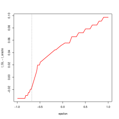
Figure 2: (a): MISE’s as a function of ϵitalic-ϵ\epsilon. (b): ^oracle^subscriptoracle\hat{\ell}-\ell_{\text{oracle}} as a function of ϵitalic-ϵ\epsilon. The dotted lines indicate the optimal value of ϵitalic-ϵ\epsilon which is used in all simulations.

We estimate h^^\hat{h} by using (19) and we take the classical Gaussian kernel K(x)=(2π)1/2exp(x2/2)𝐾𝑥superscript2𝜋12superscript𝑥22K(x)=(2\pi)^{-1/2}\exp(-x^{2}/2). For the choice of bandwidth, we apply the GL method with the family H={1,21,,δMT1}𝐻1superscript21superscript𝛿subscript𝑀𝑇1H=\left\{1,2^{-1},\ldots,\lfloor\delta M_{T}\rfloor^{-1}\right\} for some δ>0𝛿0\delta>0 small enough when MTsubscript𝑀𝑇M_{T} is large to reduce the time of numerical simulation. We have K1=1subscriptnorm𝐾11\|K\|_{1}=1, K2=21/2π1/4subscriptnorm𝐾2superscript212superscript𝜋14\|K\|_{2}=2^{-1/2}\pi^{-1/4} and KK=K2+2subscript𝐾subscript𝐾superscriptsubscript𝐾superscript2superscript2K_{\ell}\star K_{\ell^{\prime}}=K_{\sqrt{\ell^{2}+\ell^{\prime 2}}}, hence it is not difficult to calculate in practice h^,subscript^superscript\hat{h}_{\ell,\ell^{\prime}} as well as h^subscript^superscript\hat{h}_{\ell^{\prime}}. Finally, the value of ϵitalic-ϵ\epsilon in χ=(1+ϵ)(1+K1)𝜒1italic-ϵ1subscriptnorm𝐾1\chi=(1+\epsilon)(1+\|K\|_{1}) is chosen to find an optimal value of the MISE. To do this, we implement a preliminary simulation to calibrate ϵitalic-ϵ\epsilon in which we choose ϵ>1italic-ϵ1\epsilon>-1 to ensure that 1+ϵ>01italic-ϵ01+\epsilon>0. We compute the MISE and ^oracle^subscriptoracle\hat{\ell}-\ell_{\text{oracle}} as functions of ϵitalic-ϵ\epsilon where oracle=argminH𝔼[h^h22]subscript𝑜𝑟𝑎𝑐𝑙𝑒subscriptargmin𝐻𝔼delimited-[]superscriptsubscriptnormsubscript^22\ell_{oracle}=\operatorname{argmin\,}_{\ell\in H}\mathbb{E}\big{[}\|\hat{h}_{\ell}-h\|_{2}^{2}\big{]} and hh is the density of Beta(2,2)Beta22\operatorname{Beta}(2,2). In Figure 2(a), simulation results show that the risk has minimum value at ϵ=0.68italic-ϵ0.68\epsilon=-0.68. This value is not justified from a theoretical point of view. The theoretical choice ϵ>0italic-ϵ0\epsilon>0 (see Theorem 2) does not give bad results but this choice is too conservative for non-asymptotic practical purposes as often met in the literature (see Bertin et al. [9] for more details about the GL methodology). Moreover, following the discussion in Lacour and Massart [23] we investigate (see Figure 2b) the difference ^oracle^subscriptoracle\hat{\ell}-\ell_{\text{oracle}} and observe some explosions close to ϵ=0.68italic-ϵ0.68\epsilon=-0.68. Consequently, we choose ϵ=0.68italic-ϵ0.68\epsilon=-0.68 for all following simulations.

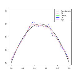
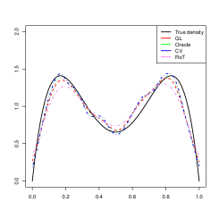
Figure 3 illustrates a reconstruction for the density of Beta(2,2)Beta22\operatorname{Beta}(2,2) and beta mixture 12Beta(2,6)+12Beta(6,2)12Beta2612Beta62\frac{1}{2}\operatorname{Beta}(2,6)+\frac{1}{2}\operatorname{Beta}(6,2) when T=13𝑇13T=13. We choose here the division rate and the growth rate R=0.5𝑅0.5R=0.5 and α=0.35𝛼0.35\alpha=0.35 respectively. We compare the estimated densities when using the GL bandwidth with those estimated with the oracle bandwidth. The oracle bandwidth is found by assuming that we know the true density. Moreover, the GL estimators are compared with estimators using the cross-validation (CV) method and the rule of thumb (RoT). The CV bandwidth is defined as follows:

CV=argminH{h^2(γ)𝑑γ2ni=1nh^,i(Γi1)}subscript𝐶𝑉𝐻argminsuperscriptsubscript^2𝛾differential-d𝛾2𝑛superscriptsubscript𝑖1𝑛subscript^𝑖subscriptsuperscriptΓ1𝑖\ell_{CV}=\underset{\ell\in H}{\operatorname{argmin\,}}\left\{\int\hat{h}_{\ell}^{2}(\gamma)d\gamma-\frac{2}{n}\sum_{i=1}^{n}\hat{h}_{\ell,-i}(\Gamma^{1}_{i})\right\}

where h^,i(γ)=1n1jiK(Γj1γ)subscript^𝑖𝛾1𝑛1subscript𝑗𝑖subscript𝐾subscriptsuperscriptΓ1𝑗𝛾\hat{h}_{\ell,-i}(\gamma)=\frac{1}{n-1}\sum_{j\neq i}K_{\ell}\big{(}\Gamma^{1}_{j}-\gamma). The RoT bandwidth can be calculated simply by using the formula RoT=1.06σ^n1/5subscript𝑅𝑜𝑇1.06^𝜎superscript𝑛15\ell_{RoT}=1.06\hat{\sigma}n^{-1/5} where σ^^𝜎\hat{\sigma} is the standard deviation of the sample (Γ11,,Γn1)subscriptsuperscriptΓ11subscriptsuperscriptΓ1𝑛(\Gamma^{1}_{1},\ldots,\Gamma^{1}_{n}). More details about these methods can be found in Section 3.4 of Silverman [32] or Tsybakov [36].

Refer to caption
(a) Reconstruction of Beta(2,2)Beta22\operatorname{Beta}(2,2)
Refer to caption
(b) Reconstruction of beta mixture
Figure 3: Reconstruction of division kernels with T=13𝑇13T=13.

To estimate the MISE, we implement Monte-Carlo simulations with respect to T=13,17𝑇1317T=13,17 and 202020. The number of repetitions for each simulation is =100100\mathcal{M}=100. Then, we compute the mean of relative error e¯=(1/)i=1ei¯𝑒1superscriptsubscript𝑖1subscript𝑒𝑖\bar{e}=(1/\mathcal{M})\sum_{i=1}^{\mathcal{M}}e_{i} and the standard deviation σe=(1/)i=1(eie¯)2subscript𝜎𝑒1superscriptsubscript𝑖1superscriptsubscript𝑒𝑖¯𝑒2\sigma_{e}=\sqrt{(1/\mathcal{M})\sum_{i=1}^{\mathcal{M}}(e_{i}-\bar{e})^{2}} where

ei=h^(i)h2h2,i=1,,,formulae-sequencesubscript𝑒𝑖subscriptnormsuperscript^𝑖2subscriptnorm2𝑖1e_{i}=\frac{\|\hat{h}^{(i)}-h\|_{2}}{\|h\|_{2}},\quad i=1,\ldots,\mathcal{M}, (33)

and h^(i)superscript^𝑖\hat{h}^{(i)} denotes the estimator of hh corresponding to ithsuperscript𝑖thi^{\text{th}} repetition.

GL Oracle CV RoT ML method
T=13𝑇13T=13 e¯¯𝑒\bar{e} 0.1001 0.0840 0.1009 0.0900 0.0610
σesubscript𝜎𝑒\sigma_{e} 0.0585 0.0481 0.0599 0.0577 0.0724
^¯¯^{\color[rgb]{1,0,0}\bar{\hat{\ell}}} 0.0920 0.0845 0.0824 0.0727
T=17𝑇17T=17 e¯¯𝑒\bar{e} 0.0458 0.0397 0.0459 0.0405 0.0166
σesubscript𝜎𝑒\sigma_{e} 0.0260 0.0230 0.0297 0.0237 0.0171
^¯¯^{\color[rgb]{1,0,0}\bar{\hat{\ell}}} 0.0485 0.0497 0.0478 0.0470
T=20𝑇20T=20 e¯¯𝑒\bar{e} 0.0261 0.0241 0.0262 0.0245 0.0088
σesubscript𝜎𝑒\sigma_{e} 0.0140 0.0114 0.0132 0.00121 0.0091
^¯¯^{\color[rgb]{1,0,0}\bar{\hat{\ell}}} 0.0377 0.0359 0.0345 0.0354
Table 1: Mean of relative error and its standard deviation for the reconstruction of Beta(2,2)Beta22\operatorname{Beta}(2,2). ^¯¯^\bar{\hat{\ell}} is the average of bandwidths for M=100𝑀100M=100 samples.
GL Oracle CV RoT
T=13𝑇13T=13 e¯¯𝑒\bar{e} 0.1361 0.1245 0.1379 0.1686
σesubscript𝜎𝑒\sigma_{e} 0.0672 0.0562 0.0815 0.0537
^¯¯^{\color[rgb]{1,0,0}\bar{\hat{\ell}}} 0.0618 0.0527 0.0522 0.0948
T=17𝑇17T=17 e¯¯𝑒\bar{e} 0.0539 0.0534 0.0550 0.0919
σesubscript𝜎𝑒\sigma_{e} 0.0180 0.0168 0.0168 0.00223
^¯¯^{\color[rgb]{1,0,0}\bar{\hat{\ell}}} 0.0309 0.0272 0.0264 0.0590
Table 2: Mean of relative error and its standard deviation for the reconstruction of beta mixture 12Beta(2,6)+12Beta(6,2)12Beta2612Beta62\frac{1}{2}\operatorname{Beta}(2,6)+\frac{1}{2}\operatorname{Beta}(6,2).

The MISE’s are computed for estimated densities using the GL bandwidth, the oracle bandwidth, the CV bandwidth and the RoT bandwidth. For a further comparison, in the reconstruction of Beta(2,2)Beta22\operatorname{Beta}(2,2), we compute the relative error in a parametric setting by comparing the true density hh with the density of Beta(a^,a^)Beta^𝑎^𝑎\operatorname{Beta}(\hat{a},\hat{a}) where a^^𝑎\hat{a} is a Maximum Likelihood (ML) estimator a𝑎a. The simulation results are displayed in Table 2 and Table 2. For the density of Beta mixture, we only compute the error with T=13𝑇13T=13 and T=17𝑇17T=17. The boxplot in Figure 4 illustrates the MISE’s in Table 2 when T=17𝑇17T=17.

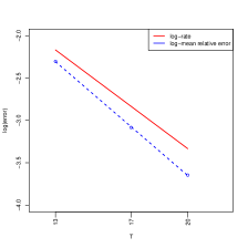
From Tables 2 and 2, we can note that the accuracy of the estimation of Beta(2,2)Beta22\operatorname{Beta}(2,2) and Beta mixture by the GL bandwidth increases for larger T𝑇T. In Figure 5, we illustrate on a log-log scale the mean relative error and the rate of convergence versus time T𝑇T. This shows that the error is close to the exponential rate predicted by the theory. Moreover, we can observe that the errors of Beta mixture are larger than those of Beta(2,2)Beta22\operatorname{Beta}(2,2) with the same T𝑇T due to the complexity of its density. In both cases, the error estimated by using oracle bandwidth is always smaller. The GL error is slightly smaller than the CV error. The RoT error can show very good behavior but lacks of stability. Overall, we conclude that the GL method has a good behavior when compared to the cross validation method and rule-of-thumb. As usual, we also see that the ML errors are quite smaller than those of nonparametric approach but the magnitude of the mean e¯¯𝑒\bar{e} remains similar.

Refer to caption
Figure 4: Errors of estimated densities of Beta(2,2)Beta22\operatorname{Beta}(2,2) when T=17𝑇17T=17.
Refer to caption
Figure 5: The log-mean relative error for the reconstruction of Beta(2,2)Beta22\operatorname{Beta}(2,2) compared to the log-rate (solid line) computed with β=1𝛽1\beta=1.

Since hh is symmetric on [0,1]01[0,1] with respect to 1212\frac{1}{2}, the estimator h^^\hat{h} can be improved and we can introduce

h~(x)=12(h^(x)+h^(1x)),~𝑥12^𝑥^1𝑥\tilde{h}(x)=\frac{1}{2}\left(\hat{h}(x)+\hat{h}(1-x)\right),

which is symmetric by construction and satisfies also (31). We compute the mean of relative error for the estimator h~~\tilde{h} with the estimation of Beta(2,2)Beta22\operatorname{Beta}(2,2) and Beta mixture. The results are displayed in Table 3. Compared with the error in Table 2 and 2, one can see as expected that the errors for the reconstruction of h~~\tilde{h} are smaller. However, these errors are of the same order, indicating that the estimator h^^\hat{h} had already good symmetric properties.

GL Oracle CV RoT
Beta(2,2)Beta22\operatorname{Beta}(2,2) T=13𝑇13T=13 0.0785 0.0634 0.0762 0.0644
T=17𝑇17T=17 0.0356 0.0309 0.0356 0.0309
Beta mixture T=13𝑇13T=13 0.1117 0.0953 0.1030 0.1584
T=17𝑇17T=17 0.0450 0.0414 0.0417 0.0893
Table 3: Mean of relative error for the reconstruction of h~~\tilde{h}.

3.2 Influence of the distribution on the mean age

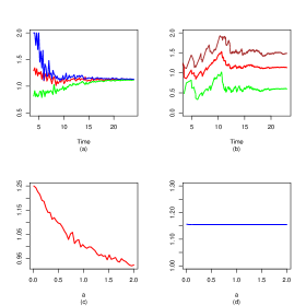
For t0𝑡0t\geq 0, recall the mean age defined in (13). To study the influence of the distribution on the mean age, we simulate n=50𝑛50n=50 trees with respect to t=6,6+t,,24𝑡66𝑡24t=6,6+\triangle t,\ldots,24 with t=0.36𝑡0.36\triangle t=0.36. For each sample (x¯t(1)subscriptsuperscript¯𝑥1𝑡\bar{x}^{(1)}_{t}, …, x¯t(n)subscriptsuperscript¯𝑥𝑛𝑡\bar{x}^{(n)}_{t}), we compute the average mean, the 1stsuperscript1st1^{\text{st}} (Q25subscript𝑄25Q_{25}) quartile and 3rdsuperscript3rd3^{\text{rd}} (Q75subscript𝑄75Q_{75}) quartile. Figure 6a and 6b show the simulation results corresponding to the density of Beta(2,2)Beta22\operatorname{Beta}(2,2) with α=0.45𝛼0.45\alpha=0.45 and R=0.4𝑅0.4R=0.4. One can see that the average of mean age and the mean age converge to αR=1.125𝛼𝑅1.125\frac{\alpha}{R}=1.125 for larger t𝑡t. This agrees with the theoretical result proved in Section 2.2.

Refer to caption
Figure 6: (a) Average mean, 1stsuperscript1st1^{\text{st}} and 3rdsuperscript3rd3^{\text{rd}} quartiles for the sample of means for 505050 trees. (b) Average mean, 1stsuperscript1st1^{\text{st}} and 3rdsuperscript3rd3^{\text{rd}} quartiles for one tree. (c) Average of Q75Q25subscript𝑄75subscript𝑄25Q_{75}-Q_{25} with a[0,2]𝑎02a\in[0,2] at t=12𝑡12t=12. (d) Mean age with a[0,2]𝑎02a\in[0,2] at t=12𝑡12t=12.

Moreover, Q25subscript𝑄25Q_{25} and Q75subscript𝑄75Q_{75} vary when the parameter a𝑎a changes. In Figure 6c, we draw a fitted curve of the average of (Q75Q25)subscript𝑄75subscript𝑄25(Q_{75}-Q_{25}) when a𝑎a varies from 00 to 222. As we mentioned in the introduction, if divisions are more asymmetric corresponding to small values of a𝑎a, the toxicities concentrate on few cells, i.e. we have more older cells after the divisions. This explains the decreasing trend in the average of (Q75Q25)subscript𝑄75subscript𝑄25(Q_{75}-Q_{25}). Finally, Figure 6d displays the average of mean ages with respect to a𝑎a. One can note that it does not change when we replace the kernel distribution, e.g Beta(0.6,0.6)Beta0.60.6\operatorname{Beta}(0.6,0.6) instead of Beta(2,2)Beta22\operatorname{Beta}(2,2).

4 Proofs

4.1 Proof of Proposition 1

ii) The proof of ii) can be found easily in literature. Here we refer to [30], Section 5.3 for this proof.
i) Let us prove that limT+NT=limj+NTj=+subscript𝑇subscript𝑁𝑇subscript𝑗subscript𝑁subscript𝑇𝑗\lim_{T\to+\infty}N_{T}=\lim_{j\to+\infty}N_{T_{j}}=+\infty. Since our model has only births and no death, (Nt)t[0,T]subscriptsubscript𝑁𝑡𝑡0𝑇(N_{t})_{t\in[0,T]} is a non-decreasing process: NTj=N0+jsubscript𝑁subscript𝑇𝑗subscript𝑁0𝑗N_{T_{j}}=N_{0}+j. All the Tjsubscript𝑇𝑗T_{j}’s are finite and limj+NTj=+subscript𝑗subscript𝑁subscript𝑇𝑗\lim_{j\to+\infty}N_{T_{j}}=+\infty a.s. From ii), we have 𝔼[NT]=N0eRT𝔼delimited-[]subscript𝑁𝑇subscript𝑁0superscript𝑒𝑅𝑇\mathbb{E}[N_{T}]=N_{0}e^{RT}. Hence, we deduce from the estimate supt[0,T]𝔼[Nt]<+𝑡0𝑇supremum𝔼delimited-[]subscript𝑁𝑡\,\underset{t\in[0,T]}{\sup}\,\mathbb{E}[N_{t}]<+\infty for all T>0𝑇0T>0 that Tjj++subscript𝑇𝑗𝑗T_{j}\underset{j\to+\infty}{\longrightarrow}+\infty a.s. Then we also have limT+NT=+subscript𝑇subscript𝑁𝑇\lim_{T\to+\infty}N_{T}=+\infty a.s.
iii) Let p=eRT𝑝superscript𝑒𝑅𝑇p=e^{-RT}. When N0=1subscript𝑁01N_{0}=1, NTGeom(p)similar-tosubscript𝑁𝑇Geom𝑝N_{T}\sim\operatorname{Geom}(p). Then we have

𝔼[1NT]𝔼delimited-[]1subscript𝑁𝑇\displaystyle\mathbb{E}\left[\frac{1}{N_{T}}\right] =n=11n(NT=n)=n=11np(1p)n1absentsuperscriptsubscript𝑛11𝑛subscript𝑁𝑇𝑛superscriptsubscript𝑛11𝑛𝑝superscript1𝑝𝑛1\displaystyle=\sum_{n=1}^{\infty}\frac{1}{n}\mathbb{P}\big{(}N_{T}=n\big{)}=\sum_{n=1}^{\infty}\frac{1}{n}p(1-p)^{n-1}
=p1pn=1+(1p)nn=p1plog(p).absent𝑝1𝑝superscriptsubscript𝑛1superscript1𝑝𝑛𝑛𝑝1𝑝𝑝\displaystyle=\frac{p}{1-p}\sum_{n=1}^{+\infty}\frac{(1-p)^{n}}{n}=-\frac{p}{1-p}\log(p).

Replace p𝑝p with eRTsuperscript𝑒𝑅𝑇e^{-RT}, we obtain (10).
When N0>1subscript𝑁01N_{0}>1, NT𝒩(N0,p)similar-tosubscript𝑁𝑇𝒩subscript𝑁0𝑝N_{T}\sim\mathcal{NB}(N_{0},p). Hence, we have

𝔼[1NT]=𝔼delimited-[]1subscript𝑁𝑇absent\displaystyle\mathbb{E}\left[\frac{1}{N_{T}}\right]= n=N01n(n1nN0)pN0(1p)nN0superscriptsubscript𝑛subscript𝑁01𝑛binomial𝑛1𝑛subscript𝑁0superscript𝑝subscript𝑁0superscript1𝑝𝑛subscript𝑁0\displaystyle\sum_{n=N_{0}}^{\infty}\frac{1}{n}\binom{n-1}{n-N_{0}}p^{N_{0}}(1-p)^{n-N_{0}}
=\displaystyle= (p1p)N0n=N01n(n1nN0)(1p)nsuperscript𝑝1𝑝subscript𝑁0superscriptsubscript𝑛subscript𝑁01𝑛binomial𝑛1𝑛subscript𝑁0superscript1𝑝𝑛\displaystyle\left(\frac{p}{1-p}\right)^{N_{0}}\sum_{n=N_{0}}^{\infty}\frac{1}{n}\binom{n-1}{n-N_{0}}(1-p)^{n}
:=:absent\displaystyle\mathrel{\mathop{\mathchar 58\relax}}= (p1p)N0f(1p),superscript𝑝1𝑝subscript𝑁0𝑓1𝑝\displaystyle\left(\frac{p}{1-p}\right)^{N_{0}}f(1-p), (34)

where f(x)=n=N0+1n(n1nN0)xn𝑓𝑥superscriptsubscript𝑛subscript𝑁01𝑛binomial𝑛1𝑛subscript𝑁0superscript𝑥𝑛f(x)=\sum_{n=N_{0}}^{+\infty}\frac{1}{n}{n-1\choose n-N_{0}}x^{n}. We can differentiate f(x)𝑓𝑥f(x) by taking derivative under the sum. Then:

ddpf(1p)=𝑑𝑑𝑝𝑓1𝑝absent\displaystyle\frac{d}{dp}f(1-p)= n=N0+(n1nN0)(1p)n1superscriptsubscript𝑛subscript𝑁0binomial𝑛1𝑛subscript𝑁0superscript1𝑝𝑛1\displaystyle-\sum_{n=N_{0}}^{+\infty}{n-1\choose n-N_{0}}(1-p)^{n-1}
=\displaystyle= (1p)N01pN0n=N0+(n1nN0)pN0(1p)nN0=1p(1p1)N01,superscript1𝑝subscript𝑁01superscript𝑝subscript𝑁0superscriptsubscript𝑛subscript𝑁0binomial𝑛1𝑛subscript𝑁0superscript𝑝subscript𝑁0superscript1𝑝𝑛subscript𝑁01𝑝superscript1𝑝1subscript𝑁01\displaystyle-\frac{(1-p)^{N_{0}-1}}{p^{N_{0}}}\sum_{n=N_{0}}^{+\infty}{n-1\choose n-N_{0}}p^{N_{0}}(1-p)^{n-N_{0}}=-\frac{1}{p}\Big{(}\frac{1}{p}-1\Big{)}^{N_{0}-1},

since the sum is 1 (we recognize the negative binomial).
Hence,

ddpf(1p)=𝑑𝑑𝑝𝑓1𝑝absent\displaystyle\frac{d}{dp}f(1-p)= 1p[k=1N01(N01k)1pk(1)N01k+(1)N01]1𝑝delimited-[]superscriptsubscript𝑘1subscript𝑁01binomialsubscript𝑁01𝑘1superscript𝑝𝑘superscript1subscript𝑁01𝑘superscript1subscript𝑁01\displaystyle-\frac{1}{p}\left[\sum_{k=1}^{N_{0}-1}\binom{N_{0}-1}{k}\frac{1}{p^{k}}(-1)^{N_{0}-1-k}+(-1)^{N_{0}-1}\right]
=\displaystyle= (1)N0[k=1N01(N01k)(1)kpk+1+1p].superscript1subscript𝑁0delimited-[]superscriptsubscript𝑘1subscript𝑁01binomialsubscript𝑁01𝑘superscript1𝑘superscript𝑝𝑘11𝑝\displaystyle(-1)^{N_{0}}\left[\sum_{k=1}^{N_{0}-1}\binom{N_{0}-1}{k}\frac{(-1)^{k}}{p^{k+1}}+\frac{1}{p}\right]. (35)

Integrating equation (35) and notice that f(0)=0𝑓00f(0)=0, we get

f(1p)=𝑓1𝑝absent\displaystyle f(1-p)= (1)N0[k=1N01(N01k)(1)kk(1pk)+log(p)]superscript1subscript𝑁0delimited-[]superscriptsubscript𝑘1subscript𝑁01binomialsubscript𝑁01𝑘superscript1𝑘𝑘1superscript𝑝𝑘𝑝\displaystyle(-1)^{N_{0}}\left[\sum_{k=1}^{N_{0}-1}\binom{N_{0}-1}{k}\frac{(-1)^{k}}{k}\Big{(}-\frac{1}{p^{k}}\Big{)}+\log(p)\right]
=\displaystyle= (1)N01[k=1N01(N01k)(1)kk1pk+log(1p)].superscript1subscript𝑁01delimited-[]superscriptsubscript𝑘1subscript𝑁01binomialsubscript𝑁01𝑘superscript1𝑘𝑘1superscript𝑝𝑘1𝑝\displaystyle(-1)^{N_{0}-1}\left[\sum_{k=1}^{N_{0}-1}\binom{N_{0}-1}{k}\frac{(-1)^{k}}{k}\frac{1}{p^{k}}+\log\left(\frac{1}{p}\right)\right]. (36)

Combine (34),(36) and replace p𝑝p with eRTsuperscript𝑒𝑅𝑇e^{-RT}, we get (11).

iv) We first prove the lower bound of (12). From (5), taking ft(x)=1subscript𝑓𝑡𝑥1f_{t}(x)=1, we have

NT=N0+0T𝟙{iNs}Q(ds,di,dγ).subscript𝑁𝑇subscript𝑁0superscriptsubscript0𝑇subscriptsubscript1𝑖subscript𝑁limit-from𝑠𝑄𝑑𝑠𝑑𝑖𝑑𝛾N_{T}=N_{0}+\int_{0}^{T}\int_{\mathcal{E}}\mathds{1}_{\{i\leq N_{s-}\}}Q(ds,di,d\gamma). (37)

Applying Itô formula for jump processes (see [20], Theorem 5.1 on p.67) to (37), we obtain

1NT1subscript𝑁𝑇\displaystyle\frac{1}{N_{T}} =1N0+0T(1Ns+11Ns)𝟙{iNs}Q(ds,di,dγ)absent1subscript𝑁0superscriptsubscript0𝑇subscript1subscript𝑁limit-from𝑠11subscript𝑁limit-from𝑠subscript1𝑖subscript𝑁limit-from𝑠𝑄𝑑𝑠𝑑𝑖𝑑𝛾\displaystyle=\frac{1}{N_{0}}+\int_{0}^{T}\int_{\mathcal{E}}\left(\frac{1}{N_{s-}+1}-\frac{1}{N_{s-}}\right)\mathds{1}_{\{i\leq N_{s-}\}}Q(ds,di,d\gamma)
=1N00T1Ns(Ns+1)𝟙{iNs}Q(ds,di,dγ).absent1subscript𝑁0superscriptsubscript0𝑇subscript1subscript𝑁limit-from𝑠subscript𝑁limit-from𝑠1subscript1𝑖subscript𝑁limit-from𝑠𝑄𝑑𝑠𝑑𝑖𝑑𝛾\displaystyle=\frac{1}{N_{0}}-\int_{0}^{T}\int_{\mathcal{E}}\frac{1}{N_{s-}\left(N_{s-}+1\right)}\mathds{1}_{\{i\leq N_{s-}\}}Q(ds,di,d\gamma).

Hence,

𝔼[1NT]=1N0𝔼[0T1Ns(Ns+1)RNs𝑑s]=1N0R0T𝔼[1Ns+1]𝑑s.𝔼delimited-[]1subscript𝑁𝑇1subscript𝑁0𝔼delimited-[]superscriptsubscript0𝑇1subscript𝑁𝑠subscript𝑁𝑠1𝑅subscript𝑁𝑠differential-d𝑠1subscript𝑁0𝑅superscriptsubscript0𝑇𝔼delimited-[]1subscript𝑁𝑠1differential-d𝑠\mathbb{E}\left[\frac{1}{N_{T}}\right]=\frac{1}{N_{0}}-\mathbb{E}\left[\int_{0}^{T}\frac{1}{N_{s}\left(N_{s}+1\right)}RN_{s}ds\right]=\frac{1}{N_{0}}-R\int_{0}^{T}\mathbb{E}\left[\frac{1}{N_{s}+1}\right]ds. (38)

Since NsN0subscript𝑁𝑠subscript𝑁0N_{s}\geq N_{0}, we have 1Ns+11Ns.1subscript𝑁𝑠11subscript𝑁𝑠\frac{1}{N_{s}+1}\leq\frac{1}{N_{s}}. Therefore, (38) implies that

𝔼[1NT]1N0R0T𝔼[1Ns]𝑑s.𝔼delimited-[]1subscript𝑁𝑇1subscript𝑁0𝑅superscriptsubscript0𝑇𝔼delimited-[]1subscript𝑁𝑠differential-d𝑠\mathbb{E}\left[\frac{1}{N_{T}}\right]\geq\frac{1}{N_{0}}-R\int_{0}^{T}\mathbb{E}\left[\frac{1}{N_{s}}\right]ds. (39)

By comparison of 𝔼[1NT]𝔼delimited-[]1subscript𝑁𝑇\mathbb{E}\left[\frac{1}{N_{T}}\right] with the solutions of the ODE ddTu(T)=Ru(T)𝑑𝑑𝑇𝑢𝑇𝑅𝑢𝑇\frac{d}{dT}u(T)=-Ru(T) with u(0)=1/N0𝑢01subscript𝑁0u(0)=1/N_{0}, we finally obtain

𝔼[1NT]1N0eRT.𝔼delimited-[]1subscript𝑁𝑇1subscript𝑁0superscript𝑒𝑅𝑇\mathbb{E}\left[\frac{1}{N_{T}}\right]\geq\frac{1}{N_{0}}e^{-RT}.

For the upper bound, notice that 𝔼[1NT]𝔼[1NT1]𝔼delimited-[]1subscript𝑁𝑇𝔼delimited-[]1subscript𝑁𝑇1\mathbb{E}\big{[}\frac{1}{N_{T}}\big{]}\leq\mathbb{E}\left[\frac{1}{N_{T}-1}\right] for N0>1subscript𝑁01N_{0}>1. Then we have

𝔼[1NT1]=𝔼delimited-[]1subscript𝑁𝑇1absent\displaystyle\mathbb{E}\Big{[}\frac{1}{N_{T}-1}\Big{]}= n=N0+1n1(n1nN0)pN0(1p)nN0superscriptsubscript𝑛subscript𝑁01𝑛1binomial𝑛1𝑛subscript𝑁0superscript𝑝subscript𝑁0superscript1𝑝𝑛subscript𝑁0\displaystyle\sum_{n=N_{0}}^{+\infty}\frac{1}{n-1}\binom{n-1}{n-N_{0}}p^{N_{0}}(1-p)^{n-N_{0}}
=\displaystyle= n=N0+(n2)!(nN0)!(N01)!pN0(1p)nN0superscriptsubscript𝑛subscript𝑁0𝑛2𝑛subscript𝑁0subscript𝑁01superscript𝑝subscript𝑁0superscript1𝑝𝑛subscript𝑁0\displaystyle\sum_{n=N_{0}}^{+\infty}\frac{(n-2)!}{(n-N_{0})!(N_{0}-1)!}p^{N_{0}}(1-p)^{n-N_{0}}
=\displaystyle= pN01n=N0+(n2)!(nN0)!(N02)!pN01(1p)nN0𝑝subscript𝑁01superscriptsubscript𝑛subscript𝑁0𝑛2𝑛subscript𝑁0subscript𝑁02superscript𝑝subscript𝑁01superscript1𝑝𝑛subscript𝑁0\displaystyle\frac{p}{N_{0}-1}\sum_{n=N_{0}}^{+\infty}\frac{(n-2)!}{(n-N_{0})!(N_{0}-2)!}p^{N_{0}-1}(1-p)^{n-N_{0}}
=\displaystyle= pN01m=N01+(m1)!(m(N01))!((N01)1)!pN01(1p)m(N01)𝑝subscript𝑁01superscriptsubscript𝑚subscript𝑁01𝑚1𝑚subscript𝑁01subscript𝑁011superscript𝑝subscript𝑁01superscript1𝑝𝑚subscript𝑁01\displaystyle\frac{p}{N_{0}-1}\sum_{m=N_{0}-1}^{+\infty}\frac{(m-1)!}{(m-(N_{0}-1))!((N_{0}-1)-1)!}p^{N_{0}-1}(1-p)^{m-(N_{0}-1)}
=\displaystyle= pN01=eRTN01,𝑝subscript𝑁01superscript𝑒𝑅𝑇subscript𝑁01\displaystyle\frac{p}{N_{0}-1}=\frac{e^{-RT}}{N_{0}-1},

by changing the index in the sum (m=n1𝑚𝑛1m=n-1) and by recognizing the negative binomial with parameter (N01,p)subscript𝑁01𝑝(N_{0}-1,p). Hence, we conclude that for N0>1subscript𝑁01N_{0}>1

eRTN0𝔼[1NT]eRTN01.superscript𝑒𝑅𝑇subscript𝑁0𝔼delimited-[]1subscript𝑁𝑇superscript𝑒𝑅𝑇subscript𝑁01\frac{e^{-RT}}{N_{0}}\leq\mathbb{E}\left[\frac{1}{N_{T}}\right]\leq\frac{e^{-RT}}{N_{0}-1}.

This ends the proof of Proposition 1.

4.2 Proof of Lemma 1

By symmetry of hh with respect to 1/2121/2, we have:

Ytsubscript𝑌𝑡\displaystyle Y_{t} =Y0+0t(α+2R01(γYsYs)h(γ)𝑑γ)𝑑s+Utabsentsubscript𝑌0superscriptsubscript0𝑡𝛼2𝑅superscriptsubscript01𝛾subscript𝑌𝑠subscript𝑌𝑠𝛾differential-d𝛾differential-d𝑠subscript𝑈𝑡\displaystyle=Y_{0}+\int_{0}^{t}\left(\alpha+2R\int_{0}^{1}\left(\gamma Y_{s}-Y_{s}\right)h(\gamma)d\gamma\right)ds+U_{t}
=Y0+0t(α2RYs01γh(γ)𝑑γ)𝑑s+Utabsentsubscript𝑌0superscriptsubscript0𝑡𝛼2𝑅subscript𝑌𝑠superscriptsubscript01𝛾𝛾differential-d𝛾differential-d𝑠subscript𝑈𝑡\displaystyle=Y_{0}+\int_{0}^{t}\left(\alpha-2RY_{s}\int_{0}^{1}\gamma h(\gamma)d\gamma\right)ds+U_{t}
=Y0+0t(αRYs)𝑑s+Ut.absentsubscript𝑌0superscriptsubscript0𝑡𝛼𝑅subscript𝑌𝑠differential-d𝑠subscript𝑈𝑡\displaystyle=Y_{0}+\int_{0}^{t}\left(\alpha-RY_{s}\right)ds+U_{t}.

where Utsubscript𝑈𝑡U_{t} is a square-integrable martingale.
Let Y~t=YteRtsubscript~𝑌𝑡subscript𝑌𝑡superscript𝑒𝑅𝑡\tilde{Y}_{t}=Y_{t}e^{Rt}, Y~0=Y0subscript~𝑌0subscript𝑌0\tilde{Y}_{0}=Y_{0}. By Itô formula, we get

Y~t=Y0~+αR(eRt1)+0teRs𝑑Us.subscript~𝑌𝑡~subscript𝑌0𝛼𝑅superscript𝑒𝑅𝑡1superscriptsubscript0𝑡superscript𝑒𝑅𝑠differential-dsubscript𝑈𝑠\tilde{Y}_{t}=\tilde{Y_{0}}+\frac{\alpha}{R}\left(e^{Rt}-1\right)+\int_{0}^{t}e^{Rs}dU_{s}.

Replacing Y~tsubscript~𝑌𝑡\tilde{Y}_{t} by YteRtsubscript𝑌𝑡superscript𝑒𝑅𝑡Y_{t}e^{Rt}, we obtain

Yt=(Y0αR)eRt+αR+0teR(ts)𝑑Us.subscript𝑌𝑡subscript𝑌0𝛼𝑅superscript𝑒𝑅𝑡𝛼𝑅superscriptsubscript0𝑡superscript𝑒𝑅𝑡𝑠differential-dsubscript𝑈𝑠Y_{t}=\left(Y_{0}-\frac{\alpha}{R}\right)e^{-Rt}+\frac{\alpha}{R}+\int_{0}^{t}e^{-R(t-s)}dU_{s}.

We end the proof by taking the expectation and the limit as t+𝑡t\rightarrow+\infty of Ytsubscript𝑌𝑡Y_{t} to obtain (16) and (17).

4.3 Proof of Theorem 1

We will show that the process Y𝑌Y satisfies ergodicity and integrability assumptions in Bansaye et al. [5] (see (H1) - (H4), Section 4). More precisely:

  • 1.

    𝔼[Yt]<+𝔼delimited-[]subscript𝑌𝑡\mathbb{E}\left[Y_{t}\right]<+\infty for all t0𝑡0t\geq 0.

  • 2.

    There exists ϖ<Ritalic-ϖ𝑅\varpi<R and c>0𝑐0c>0 such that 𝔼[Yt2]<ceϖt𝔼delimited-[]superscriptsubscript𝑌𝑡2𝑐superscript𝑒italic-ϖ𝑡\mathbb{E}\left[Y_{t}^{2}\right]<ce^{\varpi t} for all t0𝑡0t\geq 0.

From (16) we note that 𝔼[Yt]<+𝔼delimited-[]subscript𝑌𝑡\mathbb{E}[Y_{t}]<+\infty for all t0𝑡0t\geq 0. To prove the second point, from (14) we have

𝔼[Yt2]𝔼delimited-[]superscriptsubscript𝑌𝑡2\displaystyle\mathbb{E}[Y_{t}^{2}] =𝔼[Y02+0t(2αYs+2R01(γ2Ys2Ys2)h(γ)𝑑γ)𝑑s]absent𝔼delimited-[]superscriptsubscript𝑌02superscriptsubscript0𝑡2𝛼subscript𝑌𝑠2𝑅superscriptsubscript01superscript𝛾2superscriptsubscript𝑌𝑠2superscriptsubscript𝑌𝑠2𝛾differential-d𝛾differential-d𝑠\displaystyle=\mathbb{E}\left[Y_{0}^{2}+\int_{0}^{t}\left(2\alpha Y_{s}+2R\int_{0}^{1}\left(\gamma^{2}Y_{s}^{2}-Y_{s}^{2}\right)h(\gamma)d\gamma\right)ds\right]
=Y02+2α0t𝔼[Ys]𝑑s2θR0t𝔼[Ys2]𝑑s,absentsuperscriptsubscript𝑌022𝛼superscriptsubscript0𝑡𝔼delimited-[]subscript𝑌𝑠differential-d𝑠2𝜃𝑅superscriptsubscript0𝑡𝔼delimited-[]superscriptsubscript𝑌𝑠2differential-d𝑠\displaystyle=Y_{0}^{2}+2\alpha\int_{0}^{t}\mathbb{E}[Y_{s}]ds-2\theta R\int_{0}^{t}\mathbb{E}[Y_{s}^{2}]ds, (40)

with θ=01(1γ2)h(γ)𝑑γ𝜃superscriptsubscript011superscript𝛾2𝛾differential-d𝛾\theta=\int_{0}^{1}(1-\gamma^{2})h(\gamma)d\gamma and 0<θ<10𝜃10<\theta<1.

Substituting 𝔼[Yt]=(Y0α/R)eRt+α/R𝔼delimited-[]subscript𝑌𝑡subscript𝑌0𝛼𝑅superscript𝑒𝑅𝑡𝛼𝑅\mathbb{E}[Y_{t}]=(Y_{0}-\alpha/R)e^{-Rt}+\alpha/R into (40), we see that 𝔼(Yt2)𝔼superscriptsubscript𝑌𝑡2\mathbb{E}(Y_{t}^{2}) solves the following equation:

d𝔼[Yt2]dt=2θR𝔼[Yt2]+(2αY02α2R)eRt+2α2R.𝑑𝔼delimited-[]superscriptsubscript𝑌𝑡2𝑑𝑡2𝜃𝑅𝔼delimited-[]superscriptsubscript𝑌𝑡22𝛼subscript𝑌02superscript𝛼2𝑅superscript𝑒𝑅𝑡2superscript𝛼2𝑅\frac{d\mathbb{E}[Y_{t}^{2}]}{dt}=-2\theta R\mathbb{E}[Y_{t}^{2}]+\left(2\alpha Y_{0}-\frac{2\alpha^{2}}{R}\right)e^{-Rt}+\frac{2\alpha^{2}}{R}. (41)

The solution of the equation (41) is:

𝔼[Yt2]=e2θRt[Y02+0te2θRs((2αY02α2R)eRs+2α2R)𝑑s].𝔼delimited-[]superscriptsubscript𝑌𝑡2superscript𝑒2𝜃𝑅𝑡delimited-[]superscriptsubscript𝑌02superscriptsubscript0𝑡superscript𝑒2𝜃𝑅𝑠2𝛼subscript𝑌02superscript𝛼2𝑅superscript𝑒𝑅𝑠2superscript𝛼2𝑅differential-d𝑠\mathbb{E}[Y_{t}^{2}]=e^{-2\theta Rt}\left[Y_{0}^{2}+\int_{0}^{t}e^{2\theta Rs}\left(\big{(}2\alpha Y_{0}-\frac{2\alpha^{2}}{R}\big{)}e^{-Rs}+\frac{2\alpha^{2}}{R}\right)ds\right]. (42)

Hence, if θ=12𝜃12\theta=\frac{1}{2}, we have

𝔼[Yt2]𝔼delimited-[]superscriptsubscript𝑌𝑡2\displaystyle\mathbb{E}[Y_{t}^{2}] =Y02eRt+(2αY02α2R)teRt+2α2R2(1eRt)absentsuperscriptsubscript𝑌02superscript𝑒𝑅𝑡2𝛼subscript𝑌02superscript𝛼2𝑅𝑡superscript𝑒𝑅𝑡2superscript𝛼2superscript𝑅21superscript𝑒𝑅𝑡\displaystyle=Y_{0}^{2}e^{-Rt}+\big{(}2\alpha Y_{0}-\frac{2\alpha^{2}}{R}\big{)}te^{-Rt}+\frac{2\alpha^{2}}{R^{2}}\left(1-e^{-Rt}\right)
Y02eRt+(2αY02α2R)e(Rθ)t+2α2R2absentsuperscriptsubscript𝑌02superscript𝑒𝑅𝑡2𝛼subscript𝑌02superscript𝛼2𝑅superscript𝑒𝑅𝜃𝑡2superscript𝛼2superscript𝑅2\displaystyle\leq Y_{0}^{2}e^{-Rt}+\big{(}2\alpha Y_{0}-\frac{2\alpha^{2}}{R}\big{)}e^{-(R-\theta)t}+\frac{2\alpha^{2}}{R^{2}}
(Y02+2αY0+2α2R+2α2R2)e(0(θR))t=c1eϖt,absentsuperscriptsubscript𝑌022𝛼subscript𝑌02superscript𝛼2𝑅2superscript𝛼2superscript𝑅2superscript𝑒0𝜃𝑅𝑡subscript𝑐1superscript𝑒italic-ϖ𝑡\displaystyle\leq\left(Y_{0}^{2}+2\alpha Y_{0}+\frac{2\alpha^{2}}{R}+\frac{2\alpha^{2}}{R^{2}}\right)e^{(0\vee(\theta-R))t}=c_{1}e^{\varpi t},

with ϖ=0(θR):=max(0,θR)\varpi=0\vee(\theta-R)\mathrel{\mathop{\mathchar 58\relax}}=\max(0,\theta-R).
If θ12𝜃12\theta\neq\frac{1}{2},

𝔼[Yt2]𝔼delimited-[]superscriptsubscript𝑌𝑡2\displaystyle\mathbb{E}[Y_{t}^{2}] =e2θRt[Y02+(2αY02α2R)0te(2θ1)Rs𝑑s+2α2R0te2θRs𝑑s]absentsuperscript𝑒2𝜃𝑅𝑡delimited-[]superscriptsubscript𝑌022𝛼subscript𝑌02superscript𝛼2𝑅superscriptsubscript0𝑡superscript𝑒2𝜃1𝑅𝑠differential-d𝑠2superscript𝛼2𝑅superscriptsubscript0𝑡superscript𝑒2𝜃𝑅𝑠differential-d𝑠\displaystyle=e^{-2\theta Rt}\left[Y_{0}^{2}+\big{(}2\alpha Y_{0}-\frac{2\alpha^{2}}{R}\big{)}\int_{0}^{t}e^{(2\theta-1)Rs}ds+\frac{2\alpha^{2}}{R}\int_{0}^{t}e^{2\theta Rs}ds\right]
=Y02e2θRt+(2αY02α2R)1(2θ1)R(eRte2θRt)absentsuperscriptsubscript𝑌02superscript𝑒2𝜃𝑅𝑡2𝛼subscript𝑌02superscript𝛼2𝑅12𝜃1𝑅superscript𝑒𝑅𝑡superscript𝑒2𝜃𝑅𝑡\displaystyle=Y_{0}^{2}e^{-2\theta Rt}+\big{(}2\alpha Y_{0}-\frac{2\alpha^{2}}{R}\big{)}\frac{1}{(2\theta-1)R}\left(e^{-Rt}-e^{-2\theta Rt}\right)
+α2θR2(1e2θRt)superscript𝛼2𝜃superscript𝑅21superscript𝑒2𝜃𝑅𝑡\displaystyle\phantom{aaaaaaaaaaaaaaaaaaaaaaaaaaaaaaaaaaaa}+\frac{\alpha^{2}}{\theta R^{2}}\left(1-e^{-2\theta Rt}\right)
(Y02+(2αY0+2α2R)1|2θ1|R+α2θR2)=c2.absentsuperscriptsubscript𝑌022𝛼subscript𝑌02superscript𝛼2𝑅12𝜃1𝑅superscript𝛼2𝜃superscript𝑅2subscript𝑐2\displaystyle\leq\left(Y_{0}^{2}+\big{(}2\alpha Y_{0}+\frac{2\alpha^{2}}{R}\big{)}\frac{1}{|2\theta-1|R}+\frac{\alpha^{2}}{\theta R^{2}}\right)=c_{2}.

Thus, if we set c=max(c1,c2)𝑐subscript𝑐1subscript𝑐2c=\max(c_{1},c_{2}) then 𝔼[Yt2]<ceϖt𝔼delimited-[]superscriptsubscript𝑌𝑡2𝑐superscript𝑒italic-ϖ𝑡\mathbb{E}\left[Y_{t}^{2}\right]<ce^{\varpi t} for all t0𝑡0t\geq 0.
The infinitesimal generator A𝐴A of Y𝑌Y is defined for 𝒞1superscript𝒞1\mathcal{C}^{1} test functions as

Af(x)=αf(x)+2R01(f(γx)f(x))h(γ)𝑑γ.𝐴𝑓𝑥𝛼superscript𝑓𝑥2𝑅superscriptsubscript01𝑓𝛾𝑥𝑓𝑥𝛾differential-d𝛾Af(x)=\alpha f^{\prime}(x)+2R\int_{0}^{1}\left(f(\gamma x)-f(x)\right)h(\gamma)d\gamma.

For V(x)=x𝑉𝑥𝑥V(x)=x and f(x)=x+1𝑓𝑥𝑥1f(x)=x+1, we have

AV(x)=αRxR2f(x)+(α+R2)𝟙{x2αR+1}.𝐴𝑉𝑥𝛼𝑅𝑥𝑅2𝑓𝑥𝛼𝑅2subscript1𝑥2𝛼𝑅1AV(x)=\alpha-Rx\leq-\frac{R}{2}f(x)+\Big{(}\alpha+\frac{R}{2}\Big{)}\mathds{1}_{\big{\{}x\leq\frac{2\alpha}{R}+1\big{\}}}.

Hence, by Theorem 5.3 of Meyn and Tweedie [26], there exists πF(+)𝜋subscript𝐹subscript\pi\in\mathcal{M}_{F}(\mathbb{R}_{+}) such that limt+E[Yt]=π,f=αRsubscript𝑡𝐸delimited-[]subscript𝑌𝑡𝜋𝑓𝛼𝑅\lim_{t\to+\infty}E[Y_{t}]=\langle\pi,f\rangle=\frac{\alpha}{R}. Finally, applying Theorem 4.2 of [5], we obtain the result

limt+Zt,fNt=π,f=αR.𝑡subscript𝑍𝑡𝑓subscript𝑁𝑡𝜋𝑓𝛼𝑅\underset{t\to+\infty}{\lim}\frac{\langle Z_{t},f\rangle}{N_{t}}=\langle\pi,f\rangle=\frac{\alpha}{R}.

4.4 Proof of Proposition 2

To prove (20), let us remark that the number of random divisions MTsubscript𝑀𝑇M_{T} is independent of (Γi1)isubscriptsuperscriptsubscriptΓ𝑖1𝑖superscript(\Gamma_{i}^{1})_{i\in\mathbb{N}^{*}}, because the division rate R𝑅R is constant and because of the construction of our stochastic process. Therefore, we have

𝔼[h^|MT]𝔼delimited-[]conditionalsubscript^subscript𝑀𝑇\displaystyle\mathbb{E}\big{[}\hat{h}_{\ell}|M_{T}\big{]} =𝔼[1MTi=1MTK(γΓi1)|MT]=MT𝔼[K(γΓ11)]MTabsent𝔼delimited-[]conditional1subscript𝑀𝑇superscriptsubscript𝑖1subscript𝑀𝑇subscript𝐾𝛾subscriptsuperscriptΓ1𝑖subscript𝑀𝑇subscript𝑀𝑇𝔼delimited-[]subscript𝐾𝛾subscriptsuperscriptΓ11subscript𝑀𝑇\displaystyle=\mathbb{E}\Big{[}\frac{1}{M_{T}}\sum_{i=1}^{M_{T}}K_{\ell}(\gamma-\Gamma^{1}_{i})\big{|}M_{T}\Big{]}=\frac{M_{T}\mathbb{E}[K_{\ell}(\gamma-\Gamma^{1}_{1})]}{M_{T}}
=𝔼[K(γΓ11)]=Kh(γ),absent𝔼delimited-[]subscript𝐾𝛾subscriptsuperscriptΓ11subscript𝐾𝛾\displaystyle=\mathbb{E}\big{[}K_{\ell}(\gamma-\Gamma^{1}_{1})\big{]}=K_{\ell}\star h(\gamma),

and 𝔼[h^]=𝔼[𝔼[h^|MT]]=Kh(γ)𝔼delimited-[]subscript^𝔼delimited-[]𝔼delimited-[]conditionalsubscript^subscript𝑀𝑇subscript𝐾𝛾\mathbb{E}\big{[}\hat{h}_{\ell}\big{]}=\mathbb{E}\left[\mathbb{E}\big{[}\hat{h}_{\ell}|M_{T}\big{]}\right]=K_{\ell}\star h(\gamma). By similar calculations as (20), we obtain (21) and (22).

To prove ii), by the Strong Law of Large Numbers, we have

1ni=1nK(γΓi1)a.s𝔼[K(γΓ11)] as n+.1𝑛superscriptsubscript𝑖1𝑛subscript𝐾𝛾subscriptsuperscriptΓ1𝑖a.s𝔼delimited-[]subscript𝐾𝛾subscriptsuperscriptΓ11 as 𝑛\frac{1}{n}\sum_{i=1}^{n}K_{\ell}(\gamma-\Gamma^{1}_{i})\overset{\text{a.s}}{\longrightarrow}\mathbb{E}\big{[}K_{\ell}(\gamma-\Gamma^{1}_{1})\big{]}\quad\text{ as }n\to+\infty.

From (6), we have limT+NT=+subscript𝑇subscript𝑁𝑇\lim_{T\to+\infty}N_{T}=+\infty (a.s). Since MT=NTN0subscript𝑀𝑇subscript𝑁𝑇subscript𝑁0M_{T}=N_{T}-N_{0} and N0subscript𝑁0N_{0} is deterministic, this yields

1MTi=1MTK(γΓi1)a.s𝔼[K(γΓ11)]=Kh(γ).1subscript𝑀𝑇superscriptsubscript𝑖1subscript𝑀𝑇subscript𝐾𝛾subscriptsuperscriptΓ1𝑖a.s𝔼delimited-[]subscript𝐾𝛾subscriptsuperscriptΓ11subscript𝐾𝛾\frac{1}{M_{T}}\sum_{i=1}^{M_{T}}K_{\ell}\big{(}\gamma-\Gamma^{1}_{i}\big{)}\overset{\text{a.s}}{\longrightarrow}\mathbb{E}\big{[}K_{\ell}(\gamma-\Gamma^{1}_{1})\big{]}=K_{\ell}\star h(\gamma).

This ends the proof of Proposition 2.

4.5 Proof of Proposition 3

We have

𝔼[h^h2|MT]hKh2+𝔼[h^𝔼[h^]2|MT].𝔼delimited-[]conditionalsubscriptnormsubscript^2subscript𝑀𝑇subscriptnormsubscript𝐾2𝔼delimited-[]conditionalsubscriptnormsubscript^𝔼delimited-[]subscript^2subscript𝑀𝑇\displaystyle\mathbb{E}\big{[}\|\hat{h}_{\ell}-h\|_{2}|M_{T}\big{]}\leq\|h-K_{\ell}\star h\|_{2}+\mathbb{E}\big{[}\|\hat{h}_{\ell}-\mathbb{E}[\hat{h}_{\ell}]\|_{2}|M_{T}\big{]}.

For the variance term, using that 𝔼[h^(γ)]=𝔼[h^(γ)|MT]𝔼delimited-[]subscript^𝛾𝔼delimited-[]conditionalsubscript^𝛾subscript𝑀𝑇\mathbb{E}\big{[}\hat{h}_{\ell}(\gamma)\big{]}=\mathbb{E}\big{[}\hat{h}_{\ell}(\gamma)|M_{T}\big{]}

𝔼[h^𝔼[h^]22|MT]𝔼delimited-[]conditionalsuperscriptsubscriptnormsubscript^𝔼delimited-[]subscript^22subscript𝑀𝑇\displaystyle\mathbb{E}\big{[}\|\hat{h}_{\ell}-\mathbb{E}[\hat{h}_{\ell}]\|_{2}^{2}|M_{T}\big{]} =𝔼[|h^(γ)𝔼[h^(γ)]|2𝑑γ|MT]absent𝔼delimited-[]conditionalsubscriptsuperscriptsubscript^𝛾𝔼delimited-[]subscript^𝛾2differential-d𝛾subscript𝑀𝑇\displaystyle=\mathbb{E}\Big{[}\int_{\mathbb{R}}\big{|}\hat{h}_{\ell}(\gamma)-\mathbb{E}\big{[}\hat{h}_{\ell}(\gamma)\big{]}\big{|}^{2}d\gamma\big{|}M_{T}\Big{]}
=𝕍ar[h^(γ)|MT]𝑑γabsentsubscript𝕍𝑎𝑟delimited-[]conditionalsubscript^𝛾subscript𝑀𝑇differential-d𝛾\displaystyle=\int_{\mathbb{R}}\mathbb{V}ar\Big{[}\hat{h}_{\ell}(\gamma)\big{|}M_{T}\Big{]}d\gamma
=1MT𝕍ar[K(γΓ11)]𝑑γabsent1subscript𝑀𝑇subscript𝕍𝑎𝑟delimited-[]subscript𝐾𝛾subscriptsuperscriptΓ11differential-d𝛾\displaystyle=\frac{1}{M_{T}}\int_{\mathbb{R}}\mathbb{V}ar\Big{[}K_{\ell}(\gamma-\Gamma^{1}_{1})\Big{]}d\gamma
1MT𝔼[K2(γΓ11)]𝑑γabsent1subscript𝑀𝑇subscript𝔼delimited-[]superscriptsubscript𝐾2𝛾subscriptsuperscriptΓ11differential-d𝛾\displaystyle\leq\frac{1}{M_{T}}\int_{\mathbb{R}}\mathbb{E}\Big{[}K_{\ell}^{2}(\gamma-\Gamma^{1}_{1})\Big{]}d\gamma

By Fubini’s theorem, we get

𝔼[K2(γΓ11)]𝑑γsubscript𝔼delimited-[]superscriptsubscript𝐾2𝛾subscriptsuperscriptΓ11differential-d𝛾\displaystyle\int_{\mathbb{R}}\mathbb{E}\Big{[}K_{\ell}^{2}(\gamma-\Gamma^{1}_{1})\Big{]}d\gamma =K2(γu)h(u)𝑑u𝑑γabsentsubscriptsubscriptsubscriptsuperscript𝐾2𝛾𝑢𝑢differential-d𝑢differential-d𝛾\displaystyle=\int_{\mathbb{R}}\int_{\mathbb{R}}K^{2}_{\ell}(\gamma-u)h(u)du\,d\gamma
=h(u)(K2(γu)𝑑γ)𝑑uabsentsubscript𝑢subscriptsubscriptsuperscript𝐾2𝛾𝑢differential-d𝛾differential-d𝑢\displaystyle=\int_{\mathbb{R}}h(u)\left(\int_{\mathbb{R}}K^{2}_{\ell}(\gamma-u)d\gamma\right)du
=K22h(u)𝑑u=K22.absentsuperscriptsubscriptnormsubscript𝐾22subscript𝑢differential-d𝑢superscriptsubscriptnorm𝐾22\displaystyle=\|K_{\ell}\|_{2}^{2}\int_{\mathbb{R}}h(u)du=\frac{\|K\|_{2}^{2}}{\ell}.

Then we have

𝔼[h^𝔼[h^]22|MT]K22MT.𝔼delimited-[]conditionalsuperscriptsubscriptnormsubscript^𝔼delimited-[]subscript^22subscript𝑀𝑇superscriptsubscriptnorm𝐾22subscript𝑀𝑇\mathbb{E}\big{[}\|\hat{h}_{\ell}-\mathbb{E}[\hat{h}_{\ell}]\|_{2}^{2}|M_{T}\big{]}\leq\frac{\|K\|_{2}^{2}}{M_{T}\ell}. (43)

Hence, applying Cauchy-Schwarz’s inequality, we obtain (24). This ends the proof of Proposition 3.

4.6 Proof of Theorem 2

This proof is inspired by the proof of Doumic et al. [14]. However, our problem here is that the number of observations MTsubscript𝑀𝑇M_{T} is random. To overcome this difficulty, we work conditionally to MTsubscript𝑀𝑇M_{T} to get concentration inequalities.
Hereafter, we refer f𝑓\int f to fsubscript𝑓\int_{\mathbb{R}}f and since the support of hh is (0,1)01(0,1), we can write h(γ)𝑑γ𝛾differential-d𝛾\int h(\gamma)d\gamma instead of 01h(γ)𝑑γsuperscriptsubscript01𝛾differential-d𝛾\int_{0}^{1}h(\gamma)d\gamma. Recall that

A():=supH{h^,h^2χK2MT}+.A(\ell)\mathrel{\mathop{\mathchar 58\relax}}=\underset{\ell^{\prime}\in H}{\sup}\Big{\{}\|\hat{h}_{\ell,\ell^{\prime}}-\hat{h}_{\ell^{\prime}}\|_{2}-\frac{\chi\|K\|_{2}}{\sqrt{M_{T}\ell^{\prime}}}\Big{\}}_{+}.

Then, for any H𝐻\ell\in H, we have

h^h2A1+A2+A3,subscriptnorm^2subscript𝐴1subscript𝐴2subscript𝐴3\|\hat{h}-h\|_{2}\leq A_{1}+A_{2}+A_{3},

where

A1subscript𝐴1\displaystyle A_{1} :=h^h^^,2A()+χK2MT^,\displaystyle\mathrel{\mathop{\mathchar 58\relax}}=\|\hat{h}-\hat{h}_{\hat{\ell},\ell}\|_{2}\leq A(\ell)+\frac{\chi\|K\|_{2}}{\sqrt{M_{T}\hat{\ell}}},
A2subscript𝐴2\displaystyle A_{2} :=h^^,h^2A(^)+χK2MT,\displaystyle\mathrel{\mathop{\mathchar 58\relax}}=\|\hat{h}_{\hat{\ell},\ell}-\hat{h}_{\ell}\|_{2}\leq A(\hat{\ell})+\frac{\chi\|K\|_{2}}{\sqrt{M_{T}\ell}},
A3subscript𝐴3\displaystyle A_{3} :=h^h2.\displaystyle\mathrel{\mathop{\mathchar 58\relax}}=\|\hat{h}_{\ell}-h\|_{2}.

By definition of ^^\hat{\ell}, we have

A1+A22A()+2χK2MT,subscript𝐴1subscript𝐴22𝐴2𝜒subscriptnorm𝐾2subscript𝑀𝑇A_{1}+A_{2}\leq 2A(\ell)+2\frac{\chi\|K\|_{2}}{\sqrt{M_{T}\ell}}, (44)

and

A()𝐴\displaystyle A(\ell) supH{(h^,𝔼[h^,])(h^𝔼[h^])2\displaystyle\leq\underset{\ell^{\prime}\in H}{\sup}\left\{\|\big{(}\hat{h}_{\ell,\ell^{\prime}}-\mathbb{E}[\hat{h}_{\ell,\ell^{\prime}}]\big{)}-\big{(}\hat{h}_{\ell^{\prime}}-\mathbb{E}[\hat{h}_{\ell^{\prime}}]\big{)}\|_{2}\right.
+𝔼[h^,]𝔼[h^]2χK2MT}+\displaystyle\phantom{aaaaaaaaaaaaaaaaa}\left.+\|\mathbb{E}[\hat{h}_{\ell,\ell^{\prime}}]-\mathbb{E}[\hat{h}_{\ell^{\prime}}]\|_{2}-\frac{\chi\|K\|_{2}}{\sqrt{M_{T}\ell^{\prime}}}\right\}_{+}
ξT()+supH{𝔼[h^,]𝔼[h^]2},absentsubscript𝜉𝑇superscript𝐻supremumsubscriptnorm𝔼delimited-[]subscript^superscript𝔼delimited-[]subscript^superscript2\displaystyle\leq\xi_{T}(\ell)+\underset{\ell^{\prime}\in H}{\sup}\left\{\|\mathbb{E}[\hat{h}_{\ell,\ell^{\prime}}]-\mathbb{E}[\hat{h}_{\ell^{\prime}}]\|_{2}\right\}, (45)

where

ξT()=supH{(h^,𝔼[h^,])(h^𝔼[h^])2χK2MT}+.subscript𝜉𝑇superscript𝐻supremumsubscriptsubscriptnormsubscript^superscript𝔼delimited-[]subscript^superscriptsubscript^superscript𝔼delimited-[]subscript^superscript2𝜒subscriptnorm𝐾2subscript𝑀𝑇superscript\xi_{T}(\ell)=\underset{\ell^{\prime}\in H}{\sup}\left\{\|\big{(}\hat{h}_{\ell,\ell^{\prime}}-\mathbb{E}[\hat{h}_{\ell,\ell^{\prime}}]\big{)}-\big{(}\hat{h}_{\ell^{\prime}}-\mathbb{E}[\hat{h}_{\ell^{\prime}}]\big{)}\|_{2}-\frac{\chi\|K\|_{2}}{\sqrt{M_{T}\ell^{\prime}}}\right\}_{+}. (46)

For the term supH{𝔼[h^,]𝔼[h^]2}superscript𝐻supremumsubscriptnorm𝔼delimited-[]subscript^superscript𝔼delimited-[]subscript^superscript2\underset{\ell^{\prime}\in H}{\sup}\left\{\|\mathbb{E}[\hat{h}_{\ell,\ell^{\prime}}]-\mathbb{E}[\hat{h}_{\ell^{\prime}}]\|_{2}\right\}, we have

𝔼[h^,]𝔼delimited-[]subscript^superscript\displaystyle\mathbb{E}[\hat{h}_{\ell,\ell^{\prime}}] 𝔼[h^]=(KK)(γu)h(u)𝑑uK(γv)h(v)𝑑v𝔼delimited-[]subscript^superscriptsubscript𝐾subscript𝐾superscript𝛾𝑢𝑢differential-d𝑢subscript𝐾superscript𝛾𝑣𝑣differential-d𝑣\displaystyle-\mathbb{E}[\hat{h}_{\ell^{\prime}}]=\int\big{(}K_{\ell}\star K_{\ell^{\prime}}\big{)}(\gamma-u)h(u)du-\int K_{\ell^{\prime}}(\gamma-v)h(v)dv
=K(γut)K(t)h(u)𝑑t𝑑uK(γv)h(v)𝑑vabsentsubscript𝐾𝛾𝑢𝑡subscript𝐾superscript𝑡𝑢differential-d𝑡differential-d𝑢subscript𝐾superscript𝛾𝑣𝑣differential-d𝑣\displaystyle=\int\int K_{\ell}(\gamma-u-t)K_{\ell^{\prime}}(t)h(u)dtdu-\int K_{\ell^{\prime}}(\gamma-v)h(v)dv
=K(vu)K(γv)h(u)𝑑u𝑑vK(γv)h(v)𝑑vabsentsubscript𝐾𝑣𝑢subscript𝐾superscript𝛾𝑣𝑢differential-d𝑢differential-d𝑣subscript𝐾superscript𝛾𝑣𝑣differential-d𝑣\displaystyle=\int\int K_{\ell}(v-u)K_{\ell^{\prime}}(\gamma-v)h(u)dudv-\int K_{\ell^{\prime}}(\gamma-v)h(v)dv
=K(γv)(K(vu)h(u)𝑑uh(v))𝑑vabsentsubscript𝐾superscript𝛾𝑣subscript𝐾𝑣𝑢𝑢differential-d𝑢𝑣differential-d𝑣\displaystyle=\int K_{\ell^{\prime}}(\gamma-v)\left(\int K_{\ell}(v-u)h(u)du-h(v)\right)dv
=K(γv)(Kh(v)h(v))𝑑v.absentsubscript𝐾superscript𝛾𝑣subscript𝐾𝑣𝑣differential-d𝑣\displaystyle=\int K_{\ell^{\prime}}(\gamma-v)\left(K_{\ell}\star h(v)-h(v)\right)dv.

Hence, we derive

𝔼[h^,]𝔼[h^]2=K(Khh)2K1Khh2,subscriptnorm𝔼delimited-[]subscript^superscript𝔼delimited-[]subscript^superscript2subscriptnormsubscript𝐾superscriptsubscript𝐾2subscriptnorm𝐾1subscriptnormsubscript𝐾2\|\mathbb{E}[\hat{h}_{\ell,\ell^{\prime}}]-\mathbb{E}[\hat{h}_{\ell^{\prime}}]\|_{2}=\|K_{\ell^{\prime}}\star(K_{\ell}\star h-h)\|_{2}\leq\|K\|_{1}\|K_{\ell}\star h-h\|_{2}, (47)

where the right hand side does not depend on superscript\ell^{\prime} allowing us to take supHsuperscript𝐻supremum\,\underset{\ell^{\prime}\in H}{\sup}\, in the left hand side.

Thus, (44), (46) and (47) give

A1+A22ξT()+2K1Khh2+2χK2MT.subscript𝐴1subscript𝐴22subscript𝜉𝑇2subscriptnorm𝐾1subscriptnormsubscript𝐾22𝜒subscriptnorm𝐾2subscript𝑀𝑇A_{1}+A_{2}\leq 2\xi_{T}(\ell)+2\|K\|_{1}\|K_{\ell}\star h-h\|_{2}+2\frac{\chi\|K\|_{2}}{\sqrt{M_{T}\ell}}.

Then,

𝔼[(A1+A2)2]12𝔼[ξT2()]+12K12Khh22+12χ2K22𝔼[1MT].𝔼delimited-[]superscriptsubscript𝐴1subscript𝐴2212𝔼delimited-[]superscriptsubscript𝜉𝑇212superscriptsubscriptnorm𝐾12superscriptsubscriptnormsubscript𝐾2212superscript𝜒2superscriptsubscriptnorm𝐾22𝔼delimited-[]1subscript𝑀𝑇\mathbb{E}\left[(A_{1}+A_{2})^{2}\right]\leq 12\mathbb{E}[\xi_{T}^{2}(\ell)]+12\|K\|_{1}^{2}\|K_{\ell}\star h-h\|_{2}^{2}+12\frac{\chi^{2}\|K\|_{2}^{2}}{\ell}\mathbb{E}\left[\frac{1}{M_{T}}\right]. (48)

For the term A3subscript𝐴3A_{3}, we have from (43)

𝔼[A32]𝔼delimited-[]superscriptsubscript𝐴32\displaystyle\mathbb{E}\left[A_{3}^{2}\right] =𝔼[h^]h22+𝔼[h^𝔼[h^]22]absentsuperscriptsubscriptnorm𝔼delimited-[]subscript^22𝔼delimited-[]superscriptsubscriptnormsubscript^𝔼delimited-[]subscript^22\displaystyle=\|\mathbb{E}[\hat{h}_{\ell}]-h\|_{2}^{2}+\mathbb{E}\left[\|\hat{h}_{\ell}-\mathbb{E}[\hat{h}_{\ell}]\|_{2}^{2}\right]
Khh22+K22𝔼[1MT].absentsuperscriptsubscriptnormsubscript𝐾22superscriptsubscriptnorm𝐾22𝔼delimited-[]1subscript𝑀𝑇\displaystyle\leq\|K_{\ell}\star h-h\|_{2}^{2}+\frac{\|K\|_{2}^{2}}{\ell}\mathbb{E}\left[\frac{1}{M_{T}}\right].

Finally, replacing χ𝜒\chi by (1+ϵ)(1+K1)1italic-ϵ1subscriptnorm𝐾1(1+\epsilon)(1+\|K\|_{1}), we have for any H𝐻\ell\in H

𝔼[h^h22]2𝔼[(A1+A2)2]+2𝔼[A32]𝔼delimited-[]superscriptsubscriptnorm^222𝔼delimited-[]superscriptsubscript𝐴1subscript𝐴222𝔼delimited-[]superscriptsubscript𝐴32\displaystyle\mathbb{E}\left[\|\hat{h}-h\|_{2}^{2}\right]\leq 2\mathbb{E}\left[(A_{1}+A_{2})^{2}\right]+2\mathbb{E}\left[A_{3}^{2}\right]
24𝔼[ξT2()]+2(1+12K12)Khh22absent24𝔼delimited-[]subscriptsuperscript𝜉2𝑇2112superscriptsubscriptnorm𝐾12superscriptsubscriptnormsubscript𝐾22\displaystyle\phantom{aaa}\leq 24\mathbb{E}\left[\xi^{2}_{T}(\ell)\right]+2\left(1+12\|K\|_{1}^{2}\right)\|K_{\ell}\star h-h\|_{2}^{2}
+2(1+12(1+ϵ)2(1+K1)2)K22𝔼[1MT]2112superscript1italic-ϵ2superscript1subscriptnorm𝐾12superscriptsubscriptnorm𝐾22𝔼delimited-[]1subscript𝑀𝑇\displaystyle\phantom{aaaaaaaa}+2\Big{(}1+12(1+\epsilon)^{2}(1+\|K\|_{1})^{2}\Big{)}\frac{\|K\|_{2}^{2}}{\ell}\mathbb{E}\left[\frac{1}{M_{T}}\right]
24𝔼[ξT2()]+C1(Khh22+K22𝔼[1MT]),absent24𝔼delimited-[]subscriptsuperscript𝜉2𝑇subscript𝐶1superscriptsubscriptnormsubscript𝐾22superscriptsubscriptnorm𝐾22𝔼delimited-[]1subscript𝑀𝑇\displaystyle\phantom{aaa}\leq 24\mathbb{E}\left[\xi^{2}_{T}(\ell)\right]+C_{1}\left(\|K_{\ell}\star h-h\|_{2}^{2}+\frac{\|K\|_{2}^{2}}{\ell}\mathbb{E}\left[\frac{1}{M_{T}}\right]\right), (49)

with C1subscript𝐶1C_{1} a constant depending on ϵitalic-ϵ\epsilon and K1subscriptnorm𝐾1\|K\|_{1}.

It remains to deal with the term 𝔼[ξT2()]𝔼delimited-[]superscriptsubscript𝜉𝑇2\mathbb{E}\left[\xi_{T}^{2}(\ell)\right] where ξT()subscript𝜉𝑇\xi_{T}(\ell) is defined in (46),

ξT()subscript𝜉𝑇\displaystyle\xi_{T}(\ell) supH{h^,𝔼[h^,]2+h^𝔼[h^]2χK2MT}+absentsuperscript𝐻supremumsubscriptsubscriptnormsubscript^superscript𝔼delimited-[]subscript^superscript2subscriptnormsubscript^superscript𝔼delimited-[]subscript^superscript2𝜒subscriptnorm𝐾2subscript𝑀𝑇superscript\displaystyle\leq\,\underset{\ell^{\prime}\in H}{\sup}\,\left\{\|\hat{h}_{\ell,\ell^{\prime}}-\mathbb{E}[\hat{h}_{\ell,\ell^{\prime}}]\|_{2}+\|\hat{h}_{\ell^{\prime}}-\mathbb{E}[\hat{h}_{\ell^{\prime}}]\|_{2}-\frac{\chi\|K\|_{2}}{\sqrt{M_{T}\ell^{\prime}}}\right\}_{+}
supH{h^𝔼[h^]2K1+h^𝔼[h^]2χK2MT}+absentsuperscript𝐻supremumsubscriptsubscriptnormsubscript^superscript𝔼delimited-[]subscript^superscript2subscriptnorm𝐾1subscriptnormsubscript^superscript𝔼delimited-[]subscript^superscript2𝜒subscriptnorm𝐾2subscript𝑀𝑇superscript\displaystyle\leq\,\underset{\ell^{\prime}\in H}{\sup}\,\left\{\|\hat{h}_{\ell^{\prime}}-\mathbb{E}[\hat{h}_{\ell^{\prime}}]\|_{2}\|K\|_{1}+\|\hat{h}_{\ell^{\prime}}-\mathbb{E}[\hat{h}_{\ell^{\prime}}]\|_{2}-\frac{\chi\|K\|_{2}}{\sqrt{M_{T}\ell^{\prime}}}\right\}_{+}
supH{(1+K1)h^𝔼[h^]2(1+ϵ)(1+K1)K2MT}+absentsuperscript𝐻supremumsubscript1subscriptnorm𝐾1subscriptnormsubscript^superscript𝔼delimited-[]subscript^superscript21italic-ϵ1subscriptnorm𝐾1subscriptnorm𝐾2subscript𝑀𝑇superscript\displaystyle\leq\,\underset{\ell^{\prime}\in H}{\sup}\,\left\{\big{(}1+\|K\|_{1}\big{)}\|\hat{h}_{\ell^{\prime}}-\mathbb{E}[\hat{h}_{\ell^{\prime}}]\|_{2}-\frac{(1+\epsilon)(1+\|K\|_{1})\|K\|_{2}}{\sqrt{M_{T}\ell^{\prime}}}\right\}_{+}
(1+K1)ST,absent1subscriptnorm𝐾1subscript𝑆𝑇\displaystyle\leq(1+\|K\|_{1})S_{T},

where

ST:=supH{h^𝔼[h^]2(1+ϵ)K2MT}+.S_{T}\mathrel{\mathop{\mathchar 58\relax}}=\,\underset{\ell\in H}{\sup}\,\left\{\|\hat{h}_{\ell}-\mathbb{E}[\hat{h}_{\ell}]\|_{2}-\frac{(1+\epsilon)\|K\|_{2}}{\sqrt{M_{T}\ell}}\right\}_{+}.

Hence,

𝔼[ξT2()](1+K1)2𝔼[𝔼[ST2|MT]].𝔼delimited-[]superscriptsubscript𝜉𝑇2superscript1subscriptnorm𝐾12𝔼delimited-[]𝔼delimited-[]conditionalsuperscriptsubscript𝑆𝑇2subscript𝑀𝑇\displaystyle\mathbb{E}\big{[}\xi_{T}^{2}(\ell)\big{]}\leq(1+\|K\|_{1})^{2}\mathbb{E}\Big{[}\mathbb{E}\big{[}S_{T}^{2}|M_{T}\big{]}\Big{]}. (50)

If we show that

𝔼[ST2|MT=n]C1n,𝔼delimited-[]conditionalsuperscriptsubscript𝑆𝑇2subscript𝑀𝑇𝑛subscript𝐶1𝑛\mathbb{E}\big{[}S_{T}^{2}|M_{T}=n\big{]}\leq C_{*}\frac{1}{n}, (51)

then

𝔼[ξT2()]C(1+K1)2𝔼[1MT]𝔼delimited-[]superscriptsubscript𝜉𝑇2subscript𝐶superscript1subscriptnorm𝐾12𝔼delimited-[]1subscript𝑀𝑇\mathbb{E}\big{[}\xi_{T}^{2}(\ell)\big{]}\leq C_{*}(1+\|K\|_{1})^{2}\mathbb{E}\left[\frac{1}{M_{T}}\right] (52)

where Csubscript𝐶C_{*} is a constant.

Let us establish (51). When MT=nsubscript𝑀𝑇𝑛M_{T}=n, nfor-all𝑛superscript\forall n\in\mathbb{N}^{*}, we set

𝔼[Σn2]=𝔼[ST2|MT=n]𝔼delimited-[]subscriptsuperscriptΣ2𝑛𝔼delimited-[]conditionalsuperscriptsubscript𝑆𝑇2subscript𝑀𝑇𝑛\mathbb{E}\big{[}\Sigma^{2}_{n}\big{]}=\mathbb{E}\big{[}S_{T}^{2}|M_{T}=n\big{]}

where

Σn:=supH{Z2(1+ϵ)K2n}+,\Sigma_{n}\mathrel{\mathop{\mathchar 58\relax}}=\,\underset{\ell\in H}{\sup}\,\left\{\|Z_{\ell}\|_{2}-\frac{(1+\epsilon)\|K\|_{2}}{\sqrt{n\ell}}\right\}_{+},

with

Z=h^𝔼[h^]=1ni=1nK(γΓi1)𝔼[K(γΓi1)].subscript𝑍subscript^𝔼delimited-[]subscript^1𝑛superscriptsubscript𝑖1𝑛subscript𝐾𝛾subscriptsuperscriptΓ1𝑖𝔼delimited-[]subscript𝐾𝛾subscriptsuperscriptΓ1𝑖Z_{\ell}=\hat{h}_{\ell}-\mathbb{E}[\hat{h}_{\ell}]=\frac{1}{n}\sum_{i=1}^{n}K_{\ell}(\gamma-\Gamma^{1}_{i})-\mathbb{E}[K_{\ell}(\gamma-\Gamma^{1}_{i})].

Then,

𝔼[Σn2]𝔼delimited-[]subscriptsuperscriptΣ2𝑛\displaystyle\mathbb{E}\big{[}\Sigma^{2}_{n}\big{]} =𝔼[supH{Z2(1+ϵ)K2n}+2]absent𝔼delimited-[]𝐻supremumsuperscriptsubscriptsubscriptnormsubscript𝑍21italic-ϵsubscriptnorm𝐾2𝑛2\displaystyle=\mathbb{E}\left[\,\underset{\ell\in H}{\sup}\,\left\{\|Z_{\ell}\|_{2}-\frac{(1+\epsilon)\|K\|_{2}}{\sqrt{n\ell}}\right\}_{+}^{2}\right]
0+[supH{Z2(1+ϵ)K2n}+2x]𝑑xabsentsuperscriptsubscript0delimited-[]𝐻supremumsuperscriptsubscriptsubscriptnormsubscript𝑍21italic-ϵsubscriptnorm𝐾2𝑛2𝑥differential-d𝑥\displaystyle\leq\int_{0}^{+\infty}\mathbb{P}\left[\,\underset{\ell\in H}{\sup}\,\left\{\|Z_{\ell}\|_{2}-\frac{(1+\epsilon)\|K\|_{2}}{\sqrt{n\ell}}\right\}_{+}^{2}\geq x\right]dx
H0+[{Z2(1+ϵ)K2n}+2x]𝑑x.absentsubscript𝐻superscriptsubscript0delimited-[]superscriptsubscriptsubscriptnormsubscript𝑍21italic-ϵsubscriptnorm𝐾2𝑛2𝑥differential-d𝑥\displaystyle\leq\sum_{\ell\in H}\int_{0}^{+\infty}\mathbb{P}\left[\left\{\|Z_{\ell}\|_{2}-\frac{(1+\epsilon)\|K\|_{2}}{\sqrt{n\ell}}\right\}_{+}^{2}\geq x\right]dx.

We bound this with Talagrand’s inequality.

Let 𝒜𝒜\mathcal{A} be a countable dense subset of the unit ball of 𝕃2([0,1])subscript𝕃201\mathbb{L}_{2}([0,1]). We express the norm Z2subscriptnormsubscript𝑍2\|Z_{\ell}\|_{2} as

Z2subscriptnormsubscript𝑍2\displaystyle\|Z_{\ell}\|_{2} =supa𝒜a(γ)Z(γ)𝑑γabsent𝑎𝒜supremum𝑎𝛾subscript𝑍𝛾differential-d𝛾\displaystyle=\,\underset{a\in\mathcal{A}}{\sup}\,\int a(\gamma)Z_{\ell}(\gamma)d\gamma
=supa𝒜i=1na(γ)1n(K(γΓi1)𝔼[K(γΓi1)])𝑑γ.absent𝑎𝒜supremumsuperscriptsubscript𝑖1𝑛𝑎𝛾1𝑛subscript𝐾𝛾subscriptsuperscriptΓ1𝑖𝔼delimited-[]subscript𝐾𝛾subscriptsuperscriptΓ1𝑖differential-d𝛾\displaystyle=\,\underset{a\in\mathcal{A}}{\sup}\,\sum_{i=1}^{n}\int a(\gamma)\frac{1}{n}\left(K_{\ell}(\gamma-\Gamma^{1}_{i})-\mathbb{E}[K_{\ell}(\gamma-\Gamma^{1}_{i})]\right)d\gamma.

Let

Vi,Γ=a(γ)1n(K(γΓi1)𝔼[K(γΓi1)])𝑑γ.subscript𝑉𝑖Γ𝑎𝛾1𝑛subscript𝐾𝛾subscriptsuperscriptΓ1𝑖𝔼delimited-[]subscript𝐾𝛾subscriptsuperscriptΓ1𝑖differential-d𝛾V_{i,\Gamma}=\int a(\gamma)\frac{1}{n}\left(K_{\ell}(\gamma-\Gamma^{1}_{i})-\mathbb{E}[K_{\ell}(\gamma-\Gamma^{1}_{i})]\right)d\gamma.

Then Vi,Γsubscript𝑉𝑖ΓV_{i,\Gamma}, i=1,,n𝑖1𝑛i=1,\ldots,n is a sequence of i.i.d random variables with zero mean. Thus, we can apply Talagrand’s inequality (see [25, p. 170]) to Z2=supa𝒜i=1nVi,Γsubscriptnormsubscript𝑍2𝑎𝒜supremumsuperscriptsubscript𝑖1𝑛subscript𝑉𝑖Γ\|Z_{\ell}\|_{2}=\,\underset{a\in\mathcal{A}}{\sup}\,\sum_{i=1}^{n}V_{i,\Gamma}. For all η,x>0𝜂𝑥0\eta,x>0, one has

(Z2(1+η)𝔼[Z2]+2νx+c(η)bx)ex,subscriptnormsubscript𝑍21𝜂𝔼delimited-[]subscriptnormsubscript𝑍22𝜈𝑥𝑐𝜂𝑏𝑥superscript𝑒𝑥\mathbb{P}\left(\|Z_{\ell}\|_{2}\geq(1+\eta)\mathbb{E}[\|Z_{\ell}\|_{2}]+\sqrt{2\nu x}+c(\eta)bx\right)\leq e^{-x},

where c(η)=1/3+η1𝑐𝜂13superscript𝜂1c(\eta)=1/3+\eta^{-1},

ν=1nsupa𝒜𝔼[(a(γ)(K(γΓ11)𝔼[K(γΓ11)])𝑑γ)2],𝜈1𝑛𝑎𝒜supremum𝔼delimited-[]superscript𝑎𝛾subscript𝐾𝛾subscriptsuperscriptΓ11𝔼delimited-[]subscript𝐾𝛾subscriptsuperscriptΓ11differential-d𝛾2\nu=\frac{1}{n}\,\underset{a\in\mathcal{A}}{\sup}\,\mathbb{E}\left[\left(\int a(\gamma)\left(K_{\ell}(\gamma-\Gamma^{1}_{1})-\mathbb{E}[K_{\ell}(\gamma-\Gamma^{1}_{1})]\right)d\gamma\right)^{2}\right],

and,

b=1nsupy(0,1),a𝒜a(γ)(K(γy)𝔼[K(γΓ11)])𝑑γ.𝑏1𝑛formulae-sequence𝑦01𝑎𝒜supremum𝑎𝛾subscript𝐾𝛾𝑦𝔼delimited-[]subscript𝐾𝛾subscriptsuperscriptΓ11differential-d𝛾b=\frac{1}{n}\,\underset{y\in(0,1),a\in\mathcal{A}}{\sup}\,\int a(\gamma)\left(K_{\ell}(\gamma-y)-\mathbb{E}[K_{\ell}(\gamma-\Gamma^{1}_{1})]\right)d\gamma.

Next, we calculate the terms 𝔼[Z2]𝔼delimited-[]subscriptnormsubscript𝑍2\mathbb{E}[\|Z_{\ell}\|_{2}], ν𝜈\nu and b𝑏b. Applying Cauchy - Schwarz’s inequality and using independence of variables, we get

𝔼[Z2]𝔼delimited-[]subscriptnormsubscript𝑍2\displaystyle\mathbb{E}\big{[}\|Z_{\ell}\|_{2}\big{]} (𝔼[Z22])1/2absentsuperscript𝔼delimited-[]superscriptsubscriptnormsubscript𝑍2212\displaystyle\leq\left(\mathbb{E}\big{[}\|Z_{\ell}\|_{2}^{2}\big{]}\right)^{1/2}
(𝔼[(1ni=1nK(γΓi1)𝔼[K(γΓi1)])2𝑑γ])1/2absentsuperscript𝔼delimited-[]superscript1𝑛superscriptsubscript𝑖1𝑛subscript𝐾𝛾subscriptsuperscriptΓ1𝑖𝔼delimited-[]subscript𝐾𝛾subscriptsuperscriptΓ1𝑖2differential-d𝛾12\displaystyle\leq\left(\mathbb{E}\left[\int\left(\frac{1}{n}\sum_{i=1}^{n}K_{\ell}(\gamma-\Gamma^{1}_{i})-\mathbb{E}[K_{\ell}(\gamma-\Gamma^{1}_{i})]\right)^{2}d\gamma\right]\right)^{1/2}
=1n(𝔼[(i=1nK(γΓi1)𝔼[K(γΓi1)])2]𝑑γ)1/2absent1𝑛superscript𝔼delimited-[]superscriptsuperscriptsubscript𝑖1𝑛subscript𝐾𝛾subscriptsuperscriptΓ1𝑖𝔼delimited-[]subscript𝐾𝛾subscriptsuperscriptΓ1𝑖2differential-d𝛾12\displaystyle=\frac{1}{n}\left(\int\mathbb{E}\left[\left(\sum_{i=1}^{n}K_{\ell}(\gamma-\Gamma^{1}_{i})-\mathbb{E}[K_{\ell}(\gamma-\Gamma^{1}_{i})]\right)^{2}\right]d\gamma\right)^{1/2}
=1n(i=1n𝔼[(K(γΓi1)𝔼[K(γΓi1)])2]dγ)1/2absent1𝑛superscriptsuperscriptsubscript𝑖1𝑛𝔼delimited-[]superscriptsubscript𝐾𝛾subscriptsuperscriptΓ1𝑖𝔼delimited-[]subscript𝐾𝛾subscriptsuperscriptΓ1𝑖2𝑑𝛾12\displaystyle=\frac{1}{n}\left(\int\sum_{i=1}^{n}\mathbb{E}\left[\left(K_{\ell}(\gamma-\Gamma^{1}_{i})-\mathbb{E}[K_{\ell}(\gamma-\Gamma^{1}_{i})]\right)^{2}\right]d\gamma\right)^{1/2}
1n(n𝔼[K(γΓ11)2]𝑑γ)1/2=K2n.absent1𝑛superscript𝑛𝔼delimited-[]subscript𝐾superscript𝛾superscriptsubscriptΓ112differential-d𝛾12subscriptnorm𝐾2𝑛\displaystyle\leq\frac{1}{n}\left(n\int\mathbb{E}\left[K_{\ell}(\gamma-\Gamma_{1}^{1})^{2}\right]d\gamma\right)^{1/2}=\frac{\|K\|_{2}}{\sqrt{n\ell}}.

For the term ν𝜈\nu, we have

ν𝜈\displaystyle\nu 1nsupa𝒜𝔼[(a(γ)K(γΓ11)𝑑γ)2]absent1𝑛𝑎𝒜supremum𝔼delimited-[]superscript𝑎𝛾subscript𝐾𝛾superscriptsubscriptΓ11differential-d𝛾2\displaystyle\leq\frac{1}{n}\,\underset{a\in\mathcal{A}}{\sup}\,\mathbb{E}\left[\left(\int a(\gamma)K_{\ell}(\gamma-\Gamma_{1}^{1})d\gamma\right)^{2}\right]
1nsupa𝒜𝔼[|K(γΓ11)|𝑑γ×a2(γ)|K(γΓ11)|𝑑γ]absent1𝑛𝑎𝒜supremum𝔼delimited-[]subscript𝐾𝛾superscriptsubscriptΓ11differential-d𝛾superscript𝑎2𝛾subscript𝐾𝛾superscriptsubscriptΓ11differential-d𝛾\displaystyle\leq\frac{1}{n}\,\underset{a\in\mathcal{A}}{\sup}\,\mathbb{E}\left[\int|K_{\ell}(\gamma-\Gamma_{1}^{1})|d\gamma\times\int a^{2}(\gamma)|K_{\ell}(\gamma-\Gamma_{1}^{1})|d\gamma\right]
K1nsupa𝒜𝔼[a2(γ)|K(γΓ11)|𝑑γ]absentsubscriptnorm𝐾1𝑛𝑎𝒜supremum𝔼delimited-[]superscript𝑎2𝛾subscript𝐾𝛾superscriptsubscriptΓ11differential-d𝛾\displaystyle\leq\frac{\|K\|_{1}}{n}\,\underset{a\in\mathcal{A}}{\sup}\,\mathbb{E}\left[\int a^{2}(\gamma)|K_{\ell}(\gamma-\Gamma_{1}^{1})|d\gamma\right]
K1nsupa𝒜a2(γ)𝔼[|K(γΓ11)|]𝑑γabsentsubscriptnorm𝐾1𝑛𝑎𝒜supremumsuperscript𝑎2𝛾𝔼delimited-[]subscript𝐾𝛾superscriptsubscriptΓ11differential-d𝛾\displaystyle\leq\frac{\|K\|_{1}}{n}\,\underset{a\in\mathcal{A}}{\sup}\,\int a^{2}(\gamma)\mathbb{E}\left[|K_{\ell}(\gamma-\Gamma_{1}^{1})|\right]d\gamma
K1nsupa𝒜a2(γ)|K(γu)|h(u)𝑑u𝑑γabsentsubscriptnorm𝐾1𝑛𝑎𝒜supremumsuperscript𝑎2𝛾subscript𝐾𝛾𝑢𝑢differential-d𝑢differential-d𝛾\displaystyle\leq\frac{\|K\|_{1}}{n}\,\underset{a\in\mathcal{A}}{\sup}\,\int\int a^{2}(\gamma)|K_{\ell}(\gamma-u)|h(u)dud\gamma
hK12n.absentsubscriptnormsuperscriptsubscriptnorm𝐾12𝑛\displaystyle\leq\frac{\|h\|_{\infty}\|K\|_{1}^{2}}{n}.

For the term b𝑏b, we have

b𝑏\displaystyle b =1nsupy(0,1)K(y)𝔼[K(Γ11)]2\displaystyle=\frac{1}{n}\,\underset{y\in(0,1)}{\sup}\,\|K_{\ell}(\cdot-y)-\mathbb{E}[K_{\ell}(\cdot-\Gamma_{1}^{1})]\|_{2}
1n(supy(0,1)K(y)2+(𝔼[K2(γΓ11)dγ])1/2)2K2n.\displaystyle\leq\frac{1}{n}\left(\,\underset{y\in(0,1)}{\sup}\,\|K_{\ell}(\cdot-y)\|_{2}+\left(\mathbb{E}\big{[}\int K_{\ell}^{2}(\gamma-\Gamma_{1}^{1})d\gamma\big{]}\right)^{1/2}\right)\leq\frac{2\|K\|_{2}}{n\sqrt{\ell}}.

So, for all η,x>0𝜂𝑥0\eta,x>0, we have

(Z2(1+η)K2n+h1/2K12xn+2c(η)K2xn)ex.subscriptnormsubscript𝑍21𝜂subscriptnorm𝐾2𝑛superscriptsubscriptnorm12subscriptnorm𝐾12𝑥𝑛2𝑐𝜂subscriptnorm𝐾2𝑥𝑛superscript𝑒𝑥\mathbb{P}\left(\|Z_{\ell}\|_{2}\geq(1+\eta)\frac{\|K\|_{2}}{\sqrt{n\ell}}+\|h\|_{\infty}^{1/2}\|K\|_{1}\sqrt{\frac{2x}{n}}+2c(\eta)\frac{\|K\|_{2}x}{n\sqrt{\ell}}\right)\leq e^{-x}.

Let Wsubscript𝑊W_{\ell} be some strictly positive weights, we apply the previous inequality to x=W+u𝑥subscript𝑊𝑢x=W_{\ell}+u for u>0𝑢0u>0. We have

(Z2(1+η)K2n\displaystyle\mathbb{P}\Bigg{(}\|Z_{\ell}\|_{2}\geq(1+\eta)\frac{\|K\|_{2}}{\sqrt{n\ell}} +h1/2K1Wn+2c(η)K2Wnsuperscriptsubscriptnorm12subscriptnorm𝐾1subscript𝑊𝑛2𝑐𝜂subscriptnorm𝐾2subscript𝑊𝑛\displaystyle+\|h\|_{\infty}^{1/2}\|K\|_{1}\sqrt{\frac{W_{\ell}}{n}}+2c(\eta)\frac{\|K\|_{2}W_{\ell}}{n\sqrt{\ell}}
+h1/2K1un+2c(η)K2un)eWu.\displaystyle\phantom{aaaa}+\|h\|_{\infty}^{1/2}\|K\|_{1}\sqrt{\frac{u}{n}}+2c(\eta)\frac{\|K\|_{2}u}{n\sqrt{\ell}}\Bigg{)}\leq e^{-W_{\ell}-u}.

If we set

Ψ=(1+η)K2n+h1/2K1Wn+2c(η)K2Wn,subscriptΨ1𝜂subscriptnorm𝐾2𝑛superscriptsubscriptnorm12subscriptnorm𝐾1subscript𝑊𝑛2𝑐𝜂subscriptnorm𝐾2subscript𝑊𝑛\Psi_{\ell}=(1+\eta)\frac{\|K\|_{2}}{\sqrt{n\ell}}+\|h\|_{\infty}^{1/2}\|K\|_{1}\sqrt{\frac{W_{\ell}}{n}}+2c(\eta)\frac{\|K\|_{2}W_{\ell}}{n\sqrt{\ell}},

then,

(Z2Ψh1/2K1un+2c(η)K2un)eWu.subscriptnormsubscript𝑍2subscriptΨsuperscriptsubscriptnorm12subscriptnorm𝐾1𝑢𝑛2𝑐𝜂subscriptnorm𝐾2𝑢𝑛superscript𝑒subscript𝑊𝑢\mathbb{P}\Big{(}\|Z_{\ell}\|_{2}-\Psi_{\ell}\geq\|h\|_{\infty}^{1/2}\|K\|_{1}\sqrt{\frac{u}{n}}+2c(\eta)\frac{\|K\|_{2}u}{n\sqrt{\ell}}\Big{)}\leq e^{-W_{\ell}-u}.

Let

Λ=𝔼[supH(Z2Ψ)+2]=0+[supH(Z2Ψ)+2x]𝑑x.Λ𝔼delimited-[]𝐻supremumsubscriptsuperscriptsubscriptnormsubscript𝑍2subscriptΨ2superscriptsubscript0delimited-[]𝐻supremumsubscriptsuperscriptsubscriptnormsubscript𝑍2subscriptΨ2𝑥differential-d𝑥\Lambda=\mathbb{E}\left[\,\underset{\ell\in H}{\sup}\,\left(\|Z_{\ell}\|_{2}-\Psi_{\ell}\right)^{2}_{+}\right]=\int_{0}^{+\infty}\mathbb{P}\left[\,\underset{\ell\in H}{\sup}\,\left(\|Z_{\ell}\|_{2}-\Psi_{\ell}\right)^{2}_{+}\geq x\right]dx.

An upper bound of ΛΛ\Lambda is given by

ΛΛ\displaystyle\Lambda H0+[(Z2Ψ)+2x]𝑑x.absentsubscript𝐻superscriptsubscript0delimited-[]subscriptsuperscriptsubscriptnorm𝑍2subscriptΨ2𝑥differential-d𝑥\displaystyle\leq\sum_{\ell\in H}\int_{0}^{+\infty}\mathbb{P}\left[\left(\|Z\|_{2}-\Psi_{\ell}\right)^{2}_{+}\geq x\right]dx.

Let us take u𝑢u such that

x=f(u)2=(h1/2K1un+2c(η)K2un)2.𝑥𝑓superscript𝑢2superscriptsuperscriptsubscriptnorm12subscriptnorm𝐾1𝑢𝑛2𝑐𝜂subscriptnorm𝐾2𝑢𝑛2x=f(u)^{2}=\left(\|h\|_{\infty}^{1/2}\|K\|_{1}\sqrt{\frac{u}{n}}+2c(\eta)\frac{\|K\|_{2}u}{n\sqrt{\ell}}\right)^{2}.

So,

dx=2f(u)(h1/2K112nu+2c(η)K2n)du.𝑑𝑥2𝑓𝑢superscriptsubscriptnorm12subscriptnorm𝐾112𝑛𝑢2𝑐𝜂subscriptnorm𝐾2𝑛𝑑𝑢dx=2f(u)\left(\|h\|_{\infty}^{1/2}\|K\|_{1}\frac{1}{2\sqrt{nu}}+2c(\eta)\frac{\|K\|_{2}}{n\sqrt{\ell}}\right)du.

Hence,

ΛΛ\displaystyle\Lambda H0+eWu2f(u)(h1/2K112nu+2c(η)K2n)𝑑uabsentsubscript𝐻superscriptsubscript0superscript𝑒subscript𝑊𝑢2𝑓𝑢superscriptsubscriptnorm12subscriptnorm𝐾112𝑛𝑢2𝑐𝜂subscriptnorm𝐾2𝑛differential-d𝑢\displaystyle\leq\sum_{\ell\in H}\int_{0}^{+\infty}e^{-W_{\ell}-u}2f(u)\left(\|h\|_{\infty}^{1/2}\|K\|_{1}\frac{1}{2\sqrt{nu}}+2c(\eta)\frac{\|K\|_{2}}{n\sqrt{\ell}}\right)du
H0+eWu2f(u)(h1/2K1un+2c(η)K2un)u1𝑑uabsentsubscript𝐻superscriptsubscript0superscript𝑒subscript𝑊𝑢2𝑓𝑢superscriptsubscriptnorm12subscriptnorm𝐾1𝑢𝑛2𝑐𝜂subscriptnorm𝐾2𝑢𝑛superscript𝑢1differential-d𝑢\displaystyle\leq\sum_{\ell\in H}\int_{0}^{+\infty}e^{-W_{\ell}-u}2f(u)\left(\|h\|_{\infty}^{1/2}\|K\|_{1}\sqrt{\frac{u}{n}}+2c(\eta)\frac{\|K\|_{2}u}{n\sqrt{\ell}}\right)u^{-1}du
2HeW0+f2(u)euu1𝑑uabsent2subscript𝐻superscript𝑒subscript𝑊superscriptsubscript0superscript𝑓2𝑢superscript𝑒𝑢superscript𝑢1differential-d𝑢\displaystyle\leq 2\sum_{\ell\in H}e^{-W_{\ell}}\int_{0}^{+\infty}f^{2}(u)e^{-u}u^{-1}du
CηHeW(hK120+eu𝑑u+K2220+ueu𝑑u)×1nabsentsubscript𝐶𝜂subscript𝐻superscript𝑒subscript𝑊subscriptnormsuperscriptsubscriptnorm𝐾12superscriptsubscript0superscript𝑒𝑢differential-d𝑢superscriptsubscriptnorm𝐾22superscript2superscriptsubscript0𝑢superscript𝑒𝑢differential-d𝑢1𝑛\displaystyle\leq C_{\eta}\sum_{\ell\in H}e^{-W_{\ell}}\left(\|h\|_{\infty}\|K\|_{1}^{2}\int_{0}^{+\infty}e^{-u}du+\frac{\|K\|_{2}^{2}}{\ell^{2}}\int_{0}^{+\infty}ue^{-u}du\right)\times\frac{1}{n}
CηHeW(hK12+K222)×1n.absentsubscript𝐶𝜂subscript𝐻superscript𝑒subscript𝑊subscriptnormsuperscriptsubscriptnorm𝐾12superscriptsubscriptnorm𝐾22superscript21𝑛\displaystyle\leq C_{\eta}\sum_{\ell\in H}e^{-W_{\ell}}\left(\|h\|_{\infty}\|K\|_{1}^{2}+\frac{\|K\|_{2}^{2}}{\ell^{2}}\right)\times\frac{1}{n}. (53)

We need to choose Wsubscript𝑊W_{\ell} and η𝜂\eta such that

𝔼[Σn2]=𝔼[supH{Z2(1+ϵ)K2n}+2]Λ.𝔼delimited-[]subscriptsuperscriptΣ2𝑛𝔼delimited-[]𝐻supremumsuperscriptsubscriptsubscriptnormsubscript𝑍21italic-ϵsubscriptnorm𝐾2𝑛2Λ\mathbb{E}\big{[}\Sigma^{2}_{n}\big{]}=\mathbb{E}\left[\,\underset{\ell\in H}{\sup}\,\left\{\|Z_{\ell}\|_{2}-\frac{(1+\epsilon)\|K\|_{2}}{\sqrt{n\ell}}\right\}_{+}^{2}\right]\leq\Lambda. (54)

Let θ>0𝜃0\theta>0, we choose

W=θ2K222hK12,subscript𝑊superscript𝜃2superscriptsubscriptnorm𝐾222subscriptnormsuperscriptsubscriptnorm𝐾12W_{\ell}=\frac{\theta^{2}\|K\|_{2}^{2}}{2\|h\|_{\infty}\|K\|_{1}^{2}\sqrt{\ell}},

the we have

Ψ=(1+η)K2n+θK22n+c(η)θ2K23hK121n.subscriptΨ1𝜂subscriptnorm𝐾2𝑛𝜃subscriptnorm𝐾22𝑛𝑐𝜂superscript𝜃2superscriptsubscriptnorm𝐾23subscriptnormsuperscriptsubscriptnorm𝐾121𝑛\Psi_{\ell}=(1+\eta)\frac{\|K\|_{2}}{\sqrt{n\ell}}+\frac{\theta\|K\|_{2}}{\sqrt{2n\sqrt{\ell}}}+\frac{c(\eta)\theta^{2}\|K\|_{2}^{3}}{\|h\|_{\infty}\|K\|_{1}^{2}}\frac{1}{n\ell}.

Obviously, the series in (53) is finite and for any H𝐻\ell\in H, since 11\ell\leq 1, we have

ΨsubscriptΨ\displaystyle\Psi_{\ell} (1+η+θ)K2n+c(η)θ2K23hK121nabsent1𝜂𝜃subscriptnorm𝐾2𝑛𝑐𝜂superscript𝜃2superscriptsubscriptnorm𝐾23subscriptnormsuperscriptsubscriptnorm𝐾121𝑛\displaystyle\leq(1+\eta+\theta)\frac{\|K\|_{2}}{\sqrt{n\ell}}+\frac{c(\eta)\theta^{2}\|K\|_{2}^{3}}{\|h\|_{\infty}\|K\|_{1}^{2}}\frac{1}{n\ell}
(1+η+θ+c(η)θ2K22hK121n)K2n.absent1𝜂𝜃𝑐𝜂superscript𝜃2superscriptsubscriptnorm𝐾22subscriptnormsuperscriptsubscriptnorm𝐾121𝑛subscriptnorm𝐾2𝑛\displaystyle\leq\left(1+\eta+\theta+\frac{c(\eta)\theta^{2}\|K\|_{2}^{2}}{\|h\|_{\infty}\|K\|_{1}^{2}}\frac{1}{\sqrt{n\ell}}\right)\frac{\|K\|_{2}}{\sqrt{n\ell}}.

Since H{1,=1,,max}H\subset\left\{\triangle^{-1},\triangle=1,\ldots,\triangle_{\max}\right\}, if we choose max=δnsubscript𝛿𝑛\triangle_{\max}=\lfloor\delta n\rfloor for some δ>0𝛿0\delta>0, then min=max1subscriptsuperscriptsubscript1\ell_{\min}=\triangle_{\max}^{-1} and we obtain

Ψ(1+η+θ+c(η)θ2K22δhK12)K2n.subscriptΨ1𝜂𝜃𝑐𝜂superscript𝜃2superscriptsubscriptnorm𝐾22𝛿subscriptnormsuperscriptsubscriptnorm𝐾12subscriptnorm𝐾2𝑛\Psi_{\ell}\leq\left(1+\eta+\theta+\frac{c(\eta)\theta^{2}\|K\|_{2}^{2}\sqrt{\delta}}{\|h\|_{\infty}\|K\|_{1}^{2}}\right)\frac{\|K\|_{2}}{\sqrt{n\ell}}.

It remains to choose η=ϵ/2𝜂italic-ϵ2\eta=\epsilon/2 and θ𝜃\theta small enough such that

θ+c(η)θ2K22δhK12=ϵ2,𝜃𝑐𝜂superscript𝜃2superscriptsubscriptnorm𝐾22𝛿subscriptnormsuperscriptsubscriptnorm𝐾12italic-ϵ2\theta+\frac{c(\eta)\theta^{2}\|K\|_{2}^{2}\sqrt{\delta}}{\|h\|_{\infty}\|K\|_{1}^{2}}=\frac{\epsilon}{2},

then

Ψ(1+ϵ)K2n,subscriptΨ1italic-ϵsubscriptnorm𝐾2𝑛\Psi_{\ell}\leq(1+\epsilon)\frac{\|K\|_{2}}{\sqrt{n\ell}},

and we get

𝔼[Σn2]C×1n,𝔼delimited-[]subscriptsuperscriptΣ2𝑛subscript𝐶1𝑛\mathbb{E}\left[\Sigma^{2}_{n}\right]\leq C_{*}\times\frac{1}{n},

where Csubscript𝐶C_{*} is a constant depending on δ𝛿\delta,ϵitalic-ϵ\epsilon,hsubscriptnorm\|h\|_{\infty},K1subscriptnorm𝐾1\|K\|_{1} and K2subscriptnorm𝐾2\|K\|_{2}. Hence, we get (52).

Combining (49) and (52), we obtain

𝔼[h^h22]C1(Khh22+K22𝔼[1MT])+C𝔼[1MT]𝔼delimited-[]superscriptsubscriptnorm^22subscript𝐶1superscriptsubscriptnormsubscript𝐾22superscriptsubscriptnorm𝐾22𝔼delimited-[]1subscript𝑀𝑇subscript𝐶𝔼delimited-[]1subscript𝑀𝑇\mathbb{E}\left[\|\hat{h}-h\|_{2}^{2}\right]\leq C_{1}\left(\|K_{\ell}\star h-h\|_{2}^{2}+\frac{\|K\|_{2}^{2}}{\ell}\mathbb{E}\left[\frac{1}{M_{T}}\right]\right)+C_{*}\mathbb{E}\left[\frac{1}{M_{T}}\right]

Moreover, since NT>N0subscript𝑁𝑇subscript𝑁0N_{T}>N_{0}, we have

𝔼[1MT]𝔼delimited-[]1subscript𝑀𝑇\displaystyle\mathbb{E}\left[\frac{1}{M_{T}}\right] =𝔼[1NTN0]=𝔼[NTNTN01NT]=𝔼[11N0NT1NT]absent𝔼delimited-[]1subscript𝑁𝑇subscript𝑁0𝔼delimited-[]subscript𝑁𝑇subscript𝑁𝑇subscript𝑁01subscript𝑁𝑇𝔼delimited-[]11subscript𝑁0subscript𝑁𝑇1subscript𝑁𝑇\displaystyle=\mathbb{E}\left[\frac{1}{N_{T}-N_{0}}\right]=\mathbb{E}\left[\frac{N_{T}}{N_{T}-N_{0}}\frac{1}{N_{T}}\right]=\mathbb{E}\left[\frac{1}{1-\frac{N_{0}}{N_{T}}}\frac{1}{N_{T}}\right]
𝔼[11N0N0+11NT]absent𝔼delimited-[]11subscript𝑁0subscript𝑁011subscript𝑁𝑇\displaystyle\leq\mathbb{E}\left[\frac{1}{1-\frac{N_{0}}{N_{0}+1}}\frac{1}{N_{T}}\right]
(N0+1)𝔼[1NT].absentsubscript𝑁01𝔼delimited-[]1subscript𝑁𝑇\displaystyle\leq(N_{0}+1)\mathbb{E}\left[\frac{1}{N_{T}}\right]. (55)

Then, using (10), (12) and (55), recall the definition of ϱ(T)1italic-ϱsuperscript𝑇1\varrho(T)^{-1} in (29), we obtain for any H𝐻\ell\in H

𝔼[h^h22]C1(Khh22+K22ϱ(T)1)+C2ϱ(T)1.𝔼delimited-[]superscriptsubscriptnorm^22subscript𝐶1superscriptsubscriptnormsubscript𝐾22superscriptsubscriptnorm𝐾22italic-ϱsuperscript𝑇1subscript𝐶2italic-ϱsuperscript𝑇1\mathbb{E}\left[\|\hat{h}-h\|_{2}^{2}\right]\leq C_{1}\left(\|K_{\ell}\star h-h\|_{2}^{2}+\frac{\|K\|_{2}^{2}}{\ell}\varrho(T)^{-1}\right)+C_{2}\varrho(T)^{-1}.

This ends the proof of Theorem 2.

4.7 Proof of Theorem 3

We begin with the bias term Khh2subscriptnormsubscript𝐾2\|K_{\ell}\star h-h\|_{2} in the right hand side of the oracle inequality (30). For any H𝐻\ell\in H and γ(0,1)𝛾01\gamma\in(0,1), let k=β𝑘𝛽k=\lfloor\beta\rfloor and b(γ)=Kh(γ)h(γ)𝑏𝛾subscript𝐾𝛾𝛾b(\gamma)=K_{\ell}\star h(\gamma)-h(\gamma), then we have

h(γ+u)=h(γ)+h(γ)u++(u)k(k1)!01(1θ)k1h(k)(γ+θu)𝑑θ.𝛾𝑢𝛾superscript𝛾𝑢superscript𝑢𝑘𝑘1superscriptsubscript01superscript1𝜃𝑘1superscript𝑘𝛾𝜃𝑢differential-d𝜃h(\gamma+u\ell)=h(\gamma)+h^{\prime}(\gamma)u\ell+\cdots+\frac{(u\ell)^{k}}{(k-1)!}\int_{0}^{1}(1-\theta)^{k-1}h^{(k)}(\gamma+\theta u\ell)d\theta.

Since K𝐾K is a kernel of order βsuperscript𝛽\beta^{*} and β(0,β)𝛽0superscript𝛽\beta\in(0,\beta^{*}), we get

b(γ)=K(u)(u)k(k1)![01(1θ)k1(h(k)(γ+θu)h(k)(γ))𝑑θ]𝑑u.𝑏𝛾𝐾𝑢superscript𝑢𝑘𝑘1delimited-[]superscriptsubscript01superscript1𝜃𝑘1superscript𝑘𝛾𝜃𝑢superscript𝑘𝛾differential-d𝜃differential-d𝑢\displaystyle b(\gamma)=\int K(u)\frac{(u\ell)^{k}}{(k-1)!}\left[\int_{0}^{1}(1-\theta)^{k-1}\left(h^{(k)}(\gamma+\theta u\ell)-h^{(k)}(\gamma)\right)d\theta\right]du.

Setting Ek,(u)=|K(u)||u|k(k1)!subscript𝐸𝑘𝑢𝐾𝑢superscript𝑢𝑘𝑘1E_{k,\ell}(u)=|K(u)|\frac{|u\ell|^{k}}{(k-1)!} for the sake of notation. Since h(β,L)𝛽𝐿h\in\mathcal{H}(\beta,L) and applying twice the generalized Minskowki’s inequality, we obtain

h𝔼[h^]22=b2(γ)𝑑γsuperscriptsubscriptnorm𝔼delimited-[]^22superscript𝑏2𝛾differential-d𝛾\displaystyle\|h-\mathbb{E}[\hat{h}]\|_{2}^{2}=\int b^{2}(\gamma)d\gamma
(Ek,(u)[01(1θ)k1|h(k)(γ+θu)h(k)(γ)|𝑑θ]𝑑u)2𝑑γabsentsuperscriptsubscript𝐸𝑘𝑢delimited-[]superscriptsubscript01superscript1𝜃𝑘1superscript𝑘𝛾𝜃𝑢superscript𝑘𝛾differential-d𝜃differential-d𝑢2differential-d𝛾\displaystyle\leq\int\left(\int E_{k,\ell}(u)\left[\int_{0}^{1}(1-\theta)^{k-1}\big{|}h^{(k)}(\gamma+\theta u\ell)-h^{(k)}(\gamma)\big{|}d\theta\right]du\right)^{2}d\gamma
(Ek,(u)[(01(1θ)k1|h(k)(γ+θu)h(k)(γ)|𝑑θ)2𝑑γ]1/2𝑑u)2absentsuperscriptsubscript𝐸𝑘𝑢superscriptdelimited-[]superscriptsuperscriptsubscript01superscript1𝜃𝑘1superscript𝑘𝛾𝜃𝑢superscript𝑘𝛾differential-d𝜃2differential-d𝛾12differential-d𝑢2\displaystyle\leq\Bigg{(}\int E_{k,\ell}(u)\left[\int\left(\int_{0}^{1}(1-\theta)^{k-1}\big{|}h^{(k)}(\gamma+\theta u\ell)-h^{(k)}(\gamma)\big{|}d\theta\right)^{2}d\gamma\right]^{1/2}du\Bigg{)}^{2}
(Ek,(u)[01(1θ)k1(|h(k)(γ+θu)h(k)(γ)|2𝑑γ)1/2𝑑θ]𝑑u)2absentsuperscriptsubscript𝐸𝑘𝑢delimited-[]superscriptsubscript01superscript1𝜃𝑘1superscriptsuperscriptsuperscript𝑘𝛾𝜃𝑢superscript𝑘𝛾2differential-d𝛾12differential-d𝜃differential-d𝑢2\displaystyle\leq\Bigg{(}\int E_{k,\ell}(u)\left[\int_{0}^{1}(1-\theta)^{k-1}\left(\int\big{|}h^{(k)}(\gamma+\theta u\ell)-h^{(k)}(\gamma)\big{|}^{2}d\gamma\right)^{1/2}d\theta\right]du\Bigg{)}^{2}
(Ek,(u)[01(1θ)k1L(θu)βk𝑑θ]𝑑u)2absentsuperscriptsubscript𝐸𝑘𝑢delimited-[]superscriptsubscript01superscript1𝜃𝑘1𝐿superscript𝜃𝑢𝛽𝑘differential-d𝜃differential-d𝑢2\displaystyle\leq\left(\int E_{k,\ell}(u)\left[\int_{0}^{1}(1-\theta)^{k-1}L(\theta u\ell)^{\beta-k}d\theta\right]du\right)^{2}
(|K(u)||u|k(k1)![01(1θ)k1L(u)βk𝑑θ]𝑑u)2absentsuperscript𝐾𝑢superscript𝑢𝑘𝑘1delimited-[]superscriptsubscript01superscript1𝜃𝑘1𝐿superscript𝑢𝛽𝑘differential-d𝜃differential-d𝑢2\displaystyle\leq\left(\int|K(u)|\frac{|u\ell|^{k}}{(k-1)!}\left[\int_{0}^{1}(1-\theta)^{k-1}L(u\ell)^{\beta-k}d\theta\right]du\right)^{2}
CK,L,β2β,absentsubscript𝐶𝐾𝐿𝛽superscript2𝛽\displaystyle\leq C_{K,L,\beta}\ell^{2\beta},

where CK,L,β=(Lk!|u|β|K(u)|𝑑u)2subscript𝐶𝐾𝐿𝛽superscript𝐿𝑘superscript𝑢𝛽𝐾𝑢differential-d𝑢2C_{K,L,\beta}=\left(\frac{L}{k!}\int|u|^{\beta}|K(u)|du\right)^{2}.

Finally, we have

𝔼[h^h22]C1infH{CK,L,β2β+K22ϱ(T)1}+C2ϱ(T)1.𝔼delimited-[]superscriptsubscriptnorm^22subscript𝐶1𝐻infimumsubscript𝐶𝐾𝐿𝛽superscript2𝛽superscriptsubscriptnorm𝐾22italic-ϱsuperscript𝑇1subscript𝐶2italic-ϱsuperscript𝑇1\mathbb{E}\left[\|\hat{h}-h\|_{2}^{2}\right]\leq C_{1}\underset{\ell\in H}{\inf}\left\{C_{K,L,\beta}\ell^{2\beta}+\frac{\|K\|_{2}^{2}}{\ell}\varrho(T)^{-1}\right\}+C_{2}\varrho(T)^{-1}. (56)

Taking the derivative of the expression inside the infH𝐻infimum\underset{\ell\in H}{\inf} of (56) with respect to \ell, we obtain the minimizer

=(K222βCK,L,β)12β+1ϱ(T)12β+1.superscriptsuperscriptsuperscriptsubscriptnorm𝐾222𝛽subscript𝐶𝐾𝐿𝛽12𝛽1italic-ϱsuperscript𝑇12𝛽1\ell^{*}=\left(\frac{\|K\|_{2}^{2}}{2\beta C_{K,L,\beta}}\right)^{\frac{1}{2\beta+1}}\varrho(T)^{-\frac{1}{2\beta+1}}.

Since the optimal bandwidth ^^\hat{\ell} is proportional to superscript\ell^{*} up to a multiplicative constant. Therefore, by substituting \ell by ^^\hat{\ell} in the right hand side of (56), we obtain

𝔼[h^h22]C3ϱ(T)2β2β+1,𝔼delimited-[]superscriptsubscriptnorm^22subscript𝐶3italic-ϱsuperscript𝑇2𝛽2𝛽1\mathbb{E}\left[\|\hat{h}-h\|_{2}^{2}\right]\leq C_{3}\varrho(T)^{-\frac{2\beta}{2\beta+1}},

with C3subscript𝐶3C_{3} a constant depending on N0subscript𝑁0N_{0}, δ𝛿\delta, ϵitalic-ϵ\epsilon, K1subscriptnorm𝐾1\|K\|_{1}, K2subscriptnorm𝐾2\|K\|_{2}, hsubscriptnorm\|h\|_{\infty}, β𝛽\beta and L𝐿L. This ends the proof of Theorem 3.

4.8 Proof of Theorem 4

For T>0𝑇0T>0, let us denote by h^Tsubscript^𝑇\hat{h}_{T} the estimator of hh. To prove the Theorem 4, we apply the general reduction scheme proposed by Tsybakov [36] (Section 2.2, p.79). We will show the existence of a family m,T={hj,T:j=0,1,,m}\mathcal{H}_{m,T}=\big{\{}h_{j,T}\mathrel{\mathop{\mathchar 58\relax}}j=0,1,\ldots,m\big{\}} such that:

  • 1)

    hj,T(β,L)subscript𝑗𝑇𝛽𝐿h_{j,T}\in\mathcal{H}(\beta,L), j=0,,m𝑗0𝑚j=0,\ldots,m.

  • 2)

    hj,Thk,T22ceβ2β+1RT, 0j<kmformulae-sequencesubscriptnormsubscript𝑗𝑇subscript𝑘𝑇22𝑐superscript𝑒𝛽2𝛽1𝑅𝑇 0𝑗𝑘𝑚\|h_{j,T}-h_{k,T}\|_{2}\geq 2c\,e^{-\frac{\beta}{2\beta+1}RT},\;0\leq j<k\leq m.

  • 3)

    1mj=1mK(Pj,P0)ϑlog(m)1𝑚superscriptsubscript𝑗1𝑚𝐾subscript𝑃𝑗subscript𝑃0italic-ϑ𝑚\dfrac{1}{m}\sum_{j=1}^{m}K(P_{j},P_{0})\leq\vartheta\log(m) for 0<ϑ<1/80italic-ϑ180<\vartheta<1/8. Pjsubscript𝑃𝑗P_{j} and P0subscript𝑃0P_{0} are the distribution of observations when the division kernels are hj,Tsubscript𝑗𝑇h_{j,T} and h0subscript0h_{0}, respectively. K(P,Q)𝐾𝑃𝑄K(P,Q) denotes the Kullback-Leibler divergence between two measures P𝑃P and Q𝑄Q:

    K(P,Q)={logdPdQdP, if PQ+, otherwise.𝐾𝑃𝑄cases𝑑𝑃𝑑𝑄𝑑𝑃much-less-than if 𝑃𝑄 otherwiseK(P,Q)=\begin{cases}\int\log\frac{dP}{dQ}dP,&\text{ if }P\ll Q\\ +\infty,&\text{ otherwise}.\end{cases}

Under the preceding conditions 1, 2, 3, Tsybakov [36] (Theorem 2.5, p.99) show that

infh^Tmaxhm,T(h^Th22c2e2β2β+1RT)C,subscript^𝑇infimumsubscript𝑚𝑇superscriptsubscriptnormsubscript^𝑇22superscript𝑐2superscript𝑒2𝛽2𝛽1𝑅𝑇superscript𝐶\underset{\hat{h}_{T}}{\inf}\,\underset{h\in\mathcal{H}_{m,T}}{\max}\,\mathbb{P}\left(\|\hat{h}_{T}-h\|_{2}^{2}\geq c^{2}e^{-\frac{2\beta}{2\beta+1}RT}\right)\geq C^{\prime}, (57)

where the infimum is taken over all estimators h^Tsubscript^𝑇\hat{h}_{T} and positive constant Csuperscript𝐶C^{\prime} is independent of T𝑇T. This will be sufficient to obtain Theorem 4 by [36, Theorem 2.7]. The proof ends with proposing a family m,Tsubscript𝑚𝑇\mathcal{H}_{m,T} and checking the assumptions 1, 2, 3.
Construction of the family m,Tsubscript𝑚𝑇\mathcal{H}_{m,T}:

The idea is construct a family of perturbations around h0subscript0h_{0} which is a symmetric density with respect to 1212\frac{1}{2} and belongs to (L2,β)𝐿2𝛽\mathcal{H}(\frac{L}{2},\beta). For the simplification, we choose h0(γ)=𝟙(0,1)(γ)subscript0𝛾subscript101𝛾h_{0}(\gamma)=\mathds{1}_{(0,1)}(\gamma).

Let c0>0subscript𝑐00c_{0}>0 be a real number, and let γ(0,1)𝛾01\gamma\in(0,1), f(γ)=LDβg(Dγ)𝑓𝛾𝐿superscript𝐷𝛽𝑔𝐷𝛾f(\gamma)=LD^{-\beta}g\left(D\gamma\right) where g𝑔g is a regular function having support (0,1)01(0,1) and g(γ)𝑑γ=0𝑔𝛾differential-d𝛾0\int g(\gamma)d\gamma=0, g(12,β)𝑔12𝛽g\in\mathcal{H}(\frac{1}{2},\beta), we define

D=c0eRT2β+1 and fk(γ)=f(γ(k1)D),𝐷subscript𝑐0superscript𝑒𝑅𝑇2𝛽1 and subscript𝑓𝑘𝛾𝑓𝛾𝑘1𝐷D=\lceil c_{0}e^{\frac{RT}{2\beta+1}}\rceil\;\text{ and }\;f_{k}(\gamma)=f\left(\gamma-\frac{(k-1)}{D}\right),

By definition, the functions fksubscript𝑓𝑘f_{k}’s have disjoint support and one can check that the functions fk(L2,β)subscript𝑓𝑘𝐿2𝛽f_{k}\in\mathcal{H}(\frac{L}{2},\beta).

Then, the function hj,Tsubscript𝑗𝑇h_{j,T} will be chosen in

𝒟={hδ(γ)=h0(γ)+c1k=1Dδkfk(γ):δ=(δ1,,δD){0,1}D},𝒟subscript𝛿𝛾subscript0𝛾subscript𝑐1superscriptsubscript𝑘1𝐷subscript𝛿𝑘subscript𝑓𝑘𝛾:𝛿subscript𝛿1subscript𝛿𝐷superscript01𝐷\mathcal{D}=\left\{h_{\delta}(\gamma)=h_{0}(\gamma)+c_{1}\sum_{k=1}^{D}\delta_{k}f_{k}(\gamma)\mathrel{\mathop{\mathchar 58\relax}}\delta=(\delta_{1},\ldots,\delta_{D})\in\{0,1\}^{D}\right\},

where

c1=min(1LDβg,1).subscript𝑐11𝐿superscript𝐷𝛽subscriptnorm𝑔1c_{1}=\min\left(\frac{1}{LD^{-\beta}\|g\|_{\infty}},1\right). (58)

We now check that hδsubscript𝛿h_{\delta} is a density, since hδ(γ)𝑑γ=h0(γ)𝑑γ=1subscript𝛿𝛾differential-d𝛾subscript0𝛾differential-d𝛾1\int h_{\delta}(\gamma)d\gamma=\int h_{0}(\gamma)d\gamma=1, it remains to verify that hδ(γ)0γsubscript𝛿𝛾0for-all𝛾h_{\delta}(\gamma)\geq 0\;\forall\,\gamma. We have

inf(0,1)hδ(γ)01infimumsubscript𝛿𝛾\displaystyle\underset{(0,1)}{\inf}h_{\delta}(\gamma) inf(0,1)h0c1k=1Dδkfkabsent01infimumsubscript0subscriptnormsubscript𝑐1superscriptsubscript𝑘1𝐷subscript𝛿𝑘subscript𝑓𝑘\displaystyle\geq\underset{(0,1)}{\inf}h_{0}-\|c_{1}\sum_{k=1}^{D}\delta_{k}f_{k}\|_{\infty}
1c1LDβmax𝑘sup𝛾|δk|g(Dγ(k1))absent1subscript𝑐1𝐿superscript𝐷𝛽𝑘𝛾supremumsubscript𝛿𝑘𝑔𝐷𝛾𝑘1\displaystyle\geq 1-c_{1}LD^{-\beta}\underset{k}{\max}\,\underset{\gamma}{\sup}\,|\delta_{k}|g\big{(}D\gamma-(k-1)\big{)}
1c1LDβg0,absent1subscript𝑐1𝐿superscript𝐷𝛽subscriptnorm𝑔0\displaystyle\geq 1-c_{1}LD^{-\beta}\|g\|_{\infty}\geq 0,

by the choice of c1subscript𝑐1c_{1}. Thus the family of densities 𝒟𝒟\mathcal{D} is well-defined.
1) The condition hj,T(β,L)subscript𝑗𝑇𝛽𝐿h_{j,T}\in\mathcal{H}(\beta,L):
Let us denote q=β𝑞𝛽q=\lfloor\beta\rfloor, then for all γ,γ(0,1)𝛾superscript𝛾01\gamma,\gamma^{\prime}\in(0,1) we have

|hδ(q)(γ)hδ(q)(γ)|superscriptsubscript𝛿𝑞𝛾superscriptsubscript𝛿𝑞superscript𝛾\displaystyle\Big{|}h_{\delta}^{(q)}(\gamma)-h_{\delta}^{(q)}(\gamma^{\prime})\Big{|} =|h0(q)(γ)h0(q)(γ)+c1k=1Dδk(fk(q)(γ)fk(q)(γ))|absentsuperscriptsubscript0𝑞𝛾superscriptsubscript0𝑞superscript𝛾subscript𝑐1superscriptsubscript𝑘1𝐷subscript𝛿𝑘superscriptsubscript𝑓𝑘𝑞𝛾superscriptsubscript𝑓𝑘𝑞superscript𝛾\displaystyle=\Big{|}h_{0}^{(q)}(\gamma)-h_{0}^{(q)}(\gamma^{\prime})+c_{1}\sum_{k=1}^{D}\delta_{k}\big{(}f_{k}^{(q)}(\gamma)-f_{k}^{(q)}(\gamma^{\prime})\big{)}\Big{|}
c1k=1D|δk||fk(q)(γ)fk(q)(γ)|absentsubscript𝑐1superscriptsubscript𝑘1𝐷subscript𝛿𝑘superscriptsubscript𝑓𝑘𝑞𝛾superscriptsubscript𝑓𝑘𝑞superscript𝛾\displaystyle\leq c_{1}\sum_{k=1}^{D}|\delta_{k}|\Big{|}f_{k}^{(q)}(\gamma)-f_{k}^{(q)}(\gamma^{\prime})\Big{|}
c1max𝑘|fk(q)(γ)fk(q)(γ)|absentsubscript𝑐1𝑘superscriptsubscript𝑓𝑘𝑞𝛾superscriptsubscript𝑓𝑘𝑞superscript𝛾\displaystyle\leq c_{1}\underset{k}{\max}\Big{|}f_{k}^{(q)}(\gamma)-f_{k}^{(q)}(\gamma^{\prime})\Big{|}
c1LDβmax𝑘Dq|g(q)(Dγ(k1))g(q)(Dγ(k1))|absentsubscript𝑐1𝐿superscript𝐷𝛽𝑘superscript𝐷𝑞superscript𝑔𝑞𝐷𝛾𝑘1superscript𝑔𝑞𝐷superscript𝛾𝑘1\displaystyle\leq c_{1}LD^{-\beta}\underset{k}{\max}\,D^{q}\Big{|}g^{(q)}(D\gamma-(k-1))-g^{(q)}(D\gamma^{\prime}-(k-1))\Big{|}
c1LDββDββ|γγ|ββL|γγ|ββ,absentsubscript𝑐1𝐿superscript𝐷𝛽𝛽superscript𝐷𝛽𝛽superscript𝛾superscript𝛾𝛽𝛽𝐿superscript𝛾superscript𝛾𝛽𝛽\displaystyle\leq c_{1}LD^{\lfloor\beta\rfloor-\beta}D^{\beta-\lfloor\beta\rfloor}|\gamma-\gamma^{\prime}|^{\beta-\lfloor\beta\rfloor}\leq L|\gamma-\gamma^{\prime}|^{\beta-\lfloor\beta\rfloor},

which is always satisfied with c1=min(1LDβg,1)subscript𝑐11𝐿superscript𝐷𝛽subscriptnorm𝑔1c_{1}=\min\left(\frac{1}{LD^{-\beta}\|g\|_{\infty}},1\right), thus hδ(L,β)subscript𝛿𝐿𝛽h_{\delta}\in\mathcal{H}(L,\beta).
2) The condition hj,Thk,T22ceβ2β+1RTsubscriptnormsubscript𝑗𝑇subscript𝑘𝑇22𝑐superscript𝑒𝛽2𝛽1𝑅𝑇\|h_{j,T}-h_{k,T}\|_{2}\geq 2c\,e^{-\frac{\beta}{2\beta+1}RT}:
For all δ,δ{0,1}D𝛿superscript𝛿superscript01𝐷\delta,\delta^{\prime}\in\{0,1\}^{D}, we have

hδhδ2subscriptnormsubscript𝛿subscriptsuperscript𝛿2\displaystyle\|h_{\delta}-h_{\delta^{\prime}}\|_{2} =[01(hδ(γ)hδ(γ))2𝑑γ]1/2=[01(c1k=1D(δkδk)fk(γ))2𝑑γ]1/2absentsuperscriptdelimited-[]superscriptsubscript01superscriptsubscript𝛿𝛾subscriptsuperscript𝛿𝛾2differential-d𝛾12superscriptdelimited-[]superscriptsubscript01superscriptsubscript𝑐1superscriptsubscript𝑘1𝐷subscript𝛿𝑘superscriptsubscript𝛿𝑘subscript𝑓𝑘𝛾2differential-d𝛾12\displaystyle=\left[\int_{0}^{1}\big{(}h_{\delta}(\gamma)-h_{\delta^{\prime}}(\gamma)\big{)}^{2}d\gamma\right]^{1/2}=\left[\int_{0}^{1}\left(c_{1}\sum_{k=1}^{D}(\delta_{k}-\delta_{k}^{\prime})f_{k}(\gamma)\right)^{2}d\gamma\right]^{1/2}
=c1[01k=1D(δkδk)2fk2(γ)dγ]1/2=c1[k=1D(δkδk)2k1DkDfk2(γ)𝑑γ]1/2absentsubscript𝑐1superscriptdelimited-[]superscriptsubscript01superscriptsubscript𝑘1𝐷superscriptsubscript𝛿𝑘superscriptsubscript𝛿𝑘2subscriptsuperscript𝑓2𝑘𝛾𝑑𝛾12subscript𝑐1superscriptdelimited-[]superscriptsubscript𝑘1𝐷superscriptsubscript𝛿𝑘superscriptsubscript𝛿𝑘2superscriptsubscript𝑘1𝐷𝑘𝐷superscriptsubscript𝑓𝑘2𝛾differential-d𝛾12\displaystyle=c_{1}\left[\int_{0}^{1}\sum_{k=1}^{D}(\delta_{k}-\delta_{k}^{\prime})^{2}f^{2}_{k}(\gamma)d\gamma\right]^{1/2}=c_{1}\left[\sum_{k=1}^{D}(\delta_{k}-\delta_{k}^{\prime})^{2}\int_{\frac{k-1}{D}}^{\frac{k}{D}}f_{k}^{2}(\gamma)d\gamma\right]^{1/2}
=c1[k=1D(δkδk)2k1DkDL2D2βg2(Dγ(k1))𝑑γ]1/2absentsubscript𝑐1superscriptdelimited-[]superscriptsubscript𝑘1𝐷superscriptsubscript𝛿𝑘superscriptsubscript𝛿𝑘2superscriptsubscript𝑘1𝐷𝑘𝐷superscript𝐿2superscript𝐷2𝛽superscript𝑔2𝐷𝛾𝑘1differential-d𝛾12\displaystyle=c_{1}\left[\sum_{k=1}^{D}(\delta_{k}-\delta_{k}^{\prime})^{2}\int_{\frac{k-1}{D}}^{\frac{k}{D}}L^{2}D^{-2\beta}g^{2}\left(D\gamma-(k-1)\right)d\gamma\right]^{1/2}
=c1LDβ1/2g2[k=1D(δkδk)2]1/2=c1LDβ1/2g2dH(δ,δ),absentsubscript𝑐1𝐿superscript𝐷𝛽12subscriptnorm𝑔2superscriptdelimited-[]superscriptsubscript𝑘1𝐷superscriptsubscript𝛿𝑘superscriptsubscript𝛿𝑘212subscript𝑐1𝐿superscript𝐷𝛽12subscriptnorm𝑔2subscript𝑑𝐻𝛿superscript𝛿\displaystyle=c_{1}LD^{-\beta-1/2}\|g\|_{2}\left[\sum_{k=1}^{D}(\delta_{k}-\delta_{k}^{\prime})^{2}\right]^{1/2}=c_{1}LD^{-\beta-1/2}\|g\|_{2}\sqrt{d_{H}(\delta,\delta^{\prime})},

where dH(δ,δ)=k=1D𝟙{δkδk}subscript𝑑𝐻𝛿superscript𝛿superscriptsubscript𝑘1𝐷1subscript𝛿𝑘superscriptsubscript𝛿𝑘d_{H}(\delta,\delta^{\prime})=\sum_{k=1}^{D}\mathds{1}\{\delta_{k}\neq\delta_{k}^{\prime}\} is the Hamming distance between δ𝛿\delta and δsuperscript𝛿\delta^{\prime}.

According to the Lemma of Varshamov-Gilbert (cf. Tsybakov [36], p.104), there exist a subset {δ(0),,δ(m)}superscript𝛿0superscript𝛿𝑚\left\{\delta^{(0)},\ldots,\delta^{(m)}\right\} of {0,1}Dsuperscript01𝐷\{0,1\}^{D} with cardinal (59) such that δ(0)=(0,,0)superscript𝛿000\delta^{(0)}=(0,\ldots,0),

m2D/8,𝑚superscript2𝐷8m\geq 2^{D/8}, (59)

and

dH(δ(j),δ(k))D8, 0j<km.formulae-sequencesubscript𝑑𝐻superscript𝛿𝑗superscript𝛿𝑘𝐷8for-all 0𝑗𝑘𝑚d_{H}(\delta^{(j)},\delta^{(k)})\geq\frac{D}{8},\;\forall\;0\leq j<k\leq m. (60)

Then, by setting hj,T(x)=hδ(j)(x)subscript𝑗𝑇𝑥subscriptsuperscript𝛿𝑗𝑥h_{j,T}(x)=h_{\delta^{(j)}}(x), j=0,,m𝑗0𝑚j=0,\ldots,m, we obtain

hj,Thk,T2subscriptnormsubscript𝑗𝑇subscript𝑘𝑇2\displaystyle\|h_{j,T}-h_{k,T}\|_{2} =c1LDβ12g2dH(δ(j),δ(k))absentsubscript𝑐1𝐿superscript𝐷𝛽12subscriptnorm𝑔2subscript𝑑𝐻superscript𝛿𝑗superscript𝛿𝑘\displaystyle=c_{1}LD^{-\beta-\frac{1}{2}}\|g\|_{2}\sqrt{d_{H}(\delta^{(j)},\delta^{(k)})}
c1LDβ1/2g2D8absentsubscript𝑐1𝐿superscript𝐷𝛽12subscriptnorm𝑔2𝐷8\displaystyle\geq c_{1}LD^{-\beta-1/2}\|g\|_{2}\sqrt{\frac{D}{8}}
c1L4g2Dβabsentsubscript𝑐1𝐿4subscriptnorm𝑔2superscript𝐷𝛽\displaystyle\geq\frac{c_{1}L}{4}\|g\|_{2}D^{-\beta}

whenever D8𝐷8D\geq 8.

Suppose that NTNTsubscript𝑁𝑇subscript𝑁superscript𝑇N_{T}\geq N_{T^{*}} where T=log(7c0)2β+1Rsuperscript𝑇7subscript𝑐02𝛽1𝑅T^{*}=\log\left(\frac{7}{c_{0}}\right)\frac{2\beta+1}{R}. Then, D8𝐷8D\geq 8 and Dβ(2c0)βeβ2β+1RTsuperscript𝐷𝛽superscript2subscript𝑐0𝛽superscript𝑒𝛽2𝛽1𝑅𝑇D^{\beta}\leq(2c_{0})^{\beta}e^{\frac{\beta}{2\beta+1}RT}. This implies:

hj,Thk,T2c1L4g2(2c0)βeβ2β+1RT,subscriptnormsubscript𝑗𝑇subscript𝑘𝑇2subscript𝑐1𝐿4subscriptnorm𝑔2superscript2subscript𝑐0𝛽superscript𝑒𝛽2𝛽1𝑅𝑇\|h_{j,T}-h_{k,T}\|_{2}\geq\frac{c_{1}L}{4}\|g\|_{2}(2c_{0})^{-\beta}e^{-\frac{\beta}{2\beta+1}RT},

But,

min(1Lg,1)c111𝐿subscriptnorm𝑔1subscript𝑐11\min\left(\frac{1}{L\|g\|_{\infty}},1\right)\leq c_{1}\leq 1

Hence, we obtain

hj,Thk,T22ceβ2β+1RT,subscriptnormsubscript𝑗𝑇subscript𝑘𝑇22𝑐superscript𝑒𝛽2𝛽1𝑅𝑇\|h_{j,T}-h_{k,T}\|_{2}\geq 2c\;e^{-\frac{\beta}{2\beta+1}RT},

where

c=min(1,Lg2)8(2c0)β.𝑐1𝐿subscriptnorm𝑔28superscript2subscript𝑐0𝛽c=\frac{\min(1,L\|g\|_{2})}{8}(2c_{0})^{-\beta}.

3) The condition 1mj=1mK(Pj,P0)ϑlog(m)1𝑚superscriptsubscript𝑗1𝑚𝐾subscript𝑃𝑗subscript𝑃0italic-ϑ𝑚\frac{1}{m}\sum_{j=1}^{m}K(P_{j},P_{0})\leq\vartheta\log(m) for 0<ϑ<1/80italic-ϑ180<\vartheta<1/8:
We need to show that for all δ{0,1}D𝛿superscript01𝐷\delta\in\{0,1\}^{D},

K(Pδ,P0)ϑlog(m),𝐾subscript𝑃𝛿subscript𝑃0italic-ϑ𝑚K(P_{\delta},P_{0})\leq\vartheta\log(m),

where

K(Pδ,P0)=𝔼[logdPδdP0|T(Z)],𝐾subscript𝑃𝛿subscript𝑃0𝔼delimited-[]evaluated-at𝑑subscript𝑃𝛿𝑑subscript𝑃0subscript𝑇𝑍K(P_{\delta},P_{0})=\mathbb{E}\left[\log\frac{dP_{\delta}}{dP_{0}}|_{\mathcal{F}_{T}}(Z)\right],

and where (Zt)t[0,T]subscriptsubscript𝑍𝑡𝑡0𝑇(Z_{t})_{t\in[0,T]} is defined in (5) with the random measure Q𝑄Q having intensity q(ds,di,dγ)=Rhδ(γ)dsn(di)dγ𝑞𝑑𝑠𝑑𝑖𝑑𝛾𝑅subscript𝛿𝛾𝑑𝑠𝑛𝑑𝑖𝑑𝛾q(ds,di,d\gamma)=Rh_{\delta}(\gamma)ds\,n(di)d\gamma.

Here, the difficulty comes from the fact that NTsubscript𝑁𝑇N_{T} is variable because the observations result from a stochastic process Ztsubscript𝑍𝑡Z_{t}. The law of these observations is not a probability distribution on a fixed nsuperscript𝑛\mathbb{R}^{n} where n𝑛n would be the sample size, but rather a probability distribution on a path space. Pδsubscript𝑃𝛿P_{\delta} is the probability distribution when the Poisson point measure Q𝑄Q has intensity Rhδ(γ)dsn(di)dγ𝑅subscript𝛿𝛾𝑑𝑠𝑛𝑑𝑖𝑑𝛾Rh_{\delta}(\gamma)ds\,n(di)d\gamma. Thus a natural tool is to use Girsanov’s theorem (see [21], Theorem 3.24, p. 159) saying that Pδsubscript𝑃𝛿P_{\delta} is absolutely continuous with respect to P0subscript𝑃0P_{0} on Tsubscript𝑇\mathcal{F}_{T} with

dPδdP0|T=𝔇Tδ,evaluated-at𝑑subscript𝑃𝛿𝑑subscript𝑃0subscript𝑇subscriptsuperscript𝔇𝛿𝑇\frac{dP_{\delta}}{dP_{0}}|_{\mathcal{F}_{T}}=\mathfrak{D}^{\delta}_{T},

where (𝔇tδ)t[0,T]subscriptsubscriptsuperscript𝔇𝛿𝑡𝑡0𝑇(\mathfrak{D}^{\delta}_{t})_{t\in[0,T]} is the unique solution of the following SDE (see Proposition 4.17 of [34] for a similar SDE):

𝔇Tδ=1+0T𝔇sδ𝟙{iNs}(hδ(γ)h0(γ)1)Q(ds,di,dγ).subscriptsuperscript𝔇𝛿𝑇1superscriptsubscript0𝑇subscriptsubscriptsuperscript𝔇𝛿limit-from𝑠subscript1𝑖subscript𝑁limit-from𝑠subscript𝛿𝛾subscript0𝛾1𝑄𝑑𝑠𝑑𝑖𝑑𝛾\mathfrak{D}^{\delta}_{T}=1+\int_{0}^{T}\int_{\mathcal{E}}\mathfrak{D}^{\delta}_{s-}\mathds{1}_{\{i\leq N_{s-}\}}\left(\frac{h_{\delta}(\gamma)}{h_{0}(\gamma)}-1\right)Q(ds,di,d\gamma). (61)

Apply Itô formula for jump processes to (61), we get

log𝔇Tδsubscriptsuperscript𝔇𝛿𝑇\displaystyle\log\mathfrak{D}^{\delta}_{T} =0T𝟙{iNs}[log(𝔇sδ(hδ(γ)h0(γ)1)𝔇sδ)log𝔇sδ]Q(ds,di,dγ)absentsuperscriptsubscript0𝑇subscriptsubscript1𝑖subscript𝑁limit-from𝑠delimited-[]subscriptsuperscript𝔇𝛿limit-from𝑠subscript𝛿𝛾subscript0𝛾1subscriptsuperscript𝔇𝛿limit-from𝑠subscriptsuperscript𝔇𝛿limit-from𝑠𝑄𝑑𝑠𝑑𝑖𝑑𝛾\displaystyle=\int_{0}^{T}\int_{\mathcal{E}}\mathds{1}_{\{i\leq N_{s-}\}}\Bigg{[}\log\Bigg{(}\mathfrak{D}^{\delta}_{s-}-\bigg{(}\frac{h_{\delta}(\gamma)}{h_{0}(\gamma)}-1\bigg{)}\mathfrak{D}^{\delta}_{s-}\Bigg{)}-\log\mathfrak{D}^{\delta}_{s-}\Bigg{]}Q(ds,di,d\gamma)
=0T𝟙{iNs}loghδ(γ)h0(γ)Q(ds,di,dγ)=i=1NTloghδ(Γi1)h0(Γi1)absentsuperscriptsubscript0𝑇subscriptsubscript1𝑖subscript𝑁limit-from𝑠subscript𝛿𝛾subscript0𝛾𝑄𝑑𝑠𝑑𝑖𝑑𝛾superscriptsubscript𝑖1subscript𝑁𝑇subscript𝛿subscriptsuperscriptΓ1𝑖subscript0subscriptsuperscriptΓ1𝑖\displaystyle=\int_{0}^{T}\int_{\mathcal{E}}\mathds{1}_{\{i\leq N_{s-}\}}\log\frac{h_{\delta}(\gamma)}{h_{0}(\gamma)}Q(ds,di,d\gamma)=\sum_{i=1}^{N_{T}}\log\frac{h_{\delta}(\Gamma^{1}_{i})}{h_{0}(\Gamma^{1}_{i})}

by definition of (Γ11,,ΓNT1)subscriptsuperscriptΓ11subscriptsuperscriptΓ1subscript𝑁𝑇(\Gamma^{1}_{1},\ldots,\Gamma^{1}_{N_{T}}).
Then,

K(Pδ,P0)𝐾subscript𝑃𝛿subscript𝑃0\displaystyle K(P_{\delta},P_{0}) =𝔼δ[log𝔇Tδ]=𝔼δ[i=1NTloghδ(Γi1)h0(Γi1)]absentsubscript𝔼𝛿delimited-[]subscriptsuperscript𝔇𝛿𝑇subscript𝔼𝛿delimited-[]superscriptsubscript𝑖1subscript𝑁𝑇subscript𝛿subscriptsuperscriptΓ1𝑖subscript0subscriptsuperscriptΓ1𝑖\displaystyle=\mathbb{E}_{\delta}\left[\log\mathfrak{D}^{\delta}_{T}\right]=\mathbb{E}_{\delta}\left[\sum_{i=1}^{N_{T}}\log\frac{h_{\delta}(\Gamma^{1}_{i})}{h_{0}(\Gamma^{1}_{i})}\right]
=𝔼[NT]𝔼δ[loghδ(Γ11)h0(Γ11)]=𝔼[NT]01hδ(γ)loghδ(γ)h0(γ)dγ.absent𝔼delimited-[]subscript𝑁𝑇subscript𝔼𝛿delimited-[]subscript𝛿subscriptsuperscriptΓ11subscript0subscriptsuperscriptΓ11𝔼delimited-[]subscript𝑁𝑇superscriptsubscript01subscript𝛿𝛾subscript𝛿𝛾subscript0𝛾𝑑𝛾\displaystyle=\mathbb{E}\left[N_{T}\right]\mathbb{E}_{\delta}\left[\log\frac{h_{\delta}(\Gamma^{1}_{1})}{h_{0}(\Gamma^{1}_{1})}\right]=\mathbb{E}\left[N_{T}\right]\int_{0}^{1}h_{\delta}(\gamma)\log\frac{h_{\delta}(\gamma)}{h_{0}(\gamma)}d\gamma.

Here, 𝔼[NT]𝔼delimited-[]subscript𝑁𝑇\mathbb{E}\left[N_{T}\right] does not depend on hδsubscript𝛿h_{\delta} and we have 𝔼[NT]=N0eRT𝔼delimited-[]subscript𝑁𝑇subscript𝑁0superscript𝑒𝑅𝑇\mathbb{E}[N_{T}]=N_{0}e^{RT}. Thus, recall the definition of hδ()subscript𝛿h_{\delta}(\cdot) and note that log(1+x)x1𝑥𝑥\log(1+x)\leq x for x>1𝑥1x>-1, we get

K(Pδ,P0)𝐾subscript𝑃𝛿subscript𝑃0\displaystyle K(P_{\delta},P_{0}) =N0eRT01hδ(γ)log(hδ(γ))𝑑γabsentsubscript𝑁0superscript𝑒𝑅𝑇superscriptsubscript01subscript𝛿𝛾subscript𝛿𝛾differential-d𝛾\displaystyle=N_{0}e^{RT}\int_{0}^{1}h_{\delta}(\gamma)\log(h_{\delta}(\gamma))d\gamma
=N0eRT01(1+c1k=1Dδkfk(γ))log(1+c1k=1Dδkfk(γ))𝑑γabsentsubscript𝑁0superscript𝑒𝑅𝑇superscriptsubscript011subscript𝑐1superscriptsubscript𝑘1𝐷subscript𝛿𝑘subscript𝑓𝑘𝛾1subscript𝑐1superscriptsubscript𝑘1𝐷subscript𝛿𝑘subscript𝑓𝑘𝛾differential-d𝛾\displaystyle=N_{0}e^{RT}\int_{0}^{1}\Big{(}1+c_{1}\sum_{k=1}^{D}\delta_{k}f_{k}(\gamma)\Big{)}\log\Big{(}1+c_{1}\sum_{k=1}^{D}\delta_{k}f_{k}(\gamma)\Big{)}d\gamma
=N0eRTk=1Dk1DkD(1+c1δkfk(γ))log(1+c1δkfk(γ))𝑑γabsentsubscript𝑁0superscript𝑒𝑅𝑇superscriptsubscript𝑘1𝐷superscriptsubscript𝑘1𝐷𝑘𝐷1subscript𝑐1subscript𝛿𝑘subscript𝑓𝑘𝛾1subscript𝑐1subscript𝛿𝑘subscript𝑓𝑘𝛾differential-d𝛾\displaystyle=N_{0}e^{RT}\sum_{k=1}^{D}\int_{\frac{k-1}{D}}^{\frac{k}{D}}\big{(}1+c_{1}\delta_{k}f_{k}(\gamma)\big{)}\log\big{(}1+c_{1}\delta_{k}f_{k}(\gamma)\big{)}d\gamma
=N0eRTk=1Dδk01/D(1+c1f(γ))log(1+c1f(γ))𝑑γabsentsubscript𝑁0superscript𝑒𝑅𝑇superscriptsubscript𝑘1𝐷subscript𝛿𝑘superscriptsubscript01𝐷1subscript𝑐1𝑓𝛾1subscript𝑐1𝑓𝛾differential-d𝛾\displaystyle=N_{0}e^{RT}\sum_{k=1}^{D}\delta_{k}\int_{0}^{1/D}\big{(}1+c_{1}f(\gamma)\big{)}\log\big{(}1+c_{1}f(\gamma)\big{)}d\gamma
N0eRTD01/D(1+c1f(γ))c1f(γ)𝑑γabsentsubscript𝑁0superscript𝑒𝑅𝑇𝐷superscriptsubscript01𝐷1subscript𝑐1𝑓𝛾subscript𝑐1𝑓𝛾differential-d𝛾\displaystyle\leq N_{0}e^{RT}D\int_{0}^{1/D}\big{(}1+c_{1}f(\gamma)\big{)}c_{1}f(\gamma)d\gamma
N0eRT[c1LDβ01/Dg(Dγ)D𝑑γ+c12L2D2β01/Dg2(Dγ)D𝑑γ]absentsubscript𝑁0superscript𝑒𝑅𝑇delimited-[]subscript𝑐1𝐿superscript𝐷𝛽superscriptsubscript01𝐷𝑔𝐷𝛾𝐷differential-d𝛾superscriptsubscript𝑐12superscript𝐿2superscript𝐷2𝛽superscriptsubscript01𝐷superscript𝑔2𝐷𝛾𝐷differential-d𝛾\displaystyle\leq N_{0}e^{RT}\left[c_{1}LD^{-\beta}\int_{0}^{1/D}g(D\gamma)Dd\gamma+c_{1}^{2}L^{2}D^{-2\beta}\int_{0}^{1/D}g^{2}(D\gamma)Dd\gamma\right]
N0eRTc12L2D2β01g2(γ)𝑑γabsentsubscript𝑁0superscript𝑒𝑅𝑇superscriptsubscript𝑐12superscript𝐿2superscript𝐷2𝛽superscriptsubscript01superscript𝑔2𝛾differential-d𝛾\displaystyle\leq N_{0}e^{RT}c_{1}^{2}L^{2}D^{-2\beta}\int_{0}^{1}g^{2}(\gamma)d\gamma
N0c12L2g22eRTc02βe2β2β+1RTabsentsubscript𝑁0superscriptsubscript𝑐12superscript𝐿2superscriptsubscriptnorm𝑔22superscript𝑒𝑅𝑇superscriptsubscript𝑐02𝛽superscript𝑒2𝛽2𝛽1𝑅𝑇\displaystyle\leq N_{0}c_{1}^{2}L^{2}\|g\|_{2}^{2}e^{RT}c_{0}^{-2\beta}e^{-\frac{2\beta}{2\beta+1}RT}
N0L2g22c02β1D since c11.formulae-sequenceabsentsubscript𝑁0superscript𝐿2superscriptsubscriptnorm𝑔22superscriptsubscript𝑐02𝛽1𝐷 since subscript𝑐11\displaystyle\leq N_{0}L^{2}\|g\|_{2}^{2}c_{0}^{-2\beta-1}D\quad\text{ since }c_{1}\leq 1.

From (59), we have m2D/8𝑚superscript2𝐷8m\geq 2^{D/8} then

D8log(m)log(2).𝐷8𝑚2D\leq\frac{8\log(m)}{\log(2)}.

Hence, if we set

c0=(8N0L2g22ϑlog(2))1/(2β+1),subscript𝑐0superscript8subscript𝑁0superscript𝐿2superscriptsubscriptnorm𝑔22italic-ϑ212𝛽1c_{0}=\left(\frac{8N_{0}L^{2}\|g\|_{2}^{2}}{\vartheta\log(2)}\right)^{1/(2\beta+1)},

we obtain K(Pδ,P0)ϑlog(m)𝐾subscript𝑃𝛿subscript𝑃0italic-ϑ𝑚K(P_{\delta},P_{0})\leq\vartheta\log(m). This ends the proof of Theorem 4.

Acknowledgements
The author is deeply grateful to V.C. Tran, V. Rivoirard and T.M. Pham Ngoc for the guidance and useful suggestions. The author would like to express his sincere thanks to P. Massart for constructive comments that improved the results. The author would like to thank Centre de Resources Informatiques de Lille 1 (CRI) for the computational cluster to implement the numerical simulations. This work is supported by Program 911 of Vietnam Ministry of Education and Training and is partly supported by the French Agence Nationale de la Recherche (ANR 2011 BS01 010 01 projet Calibration).
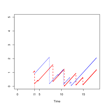
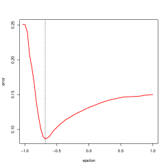
References

  • [1] H. Aguilaniu, L. Gustafsson, M. Rigoulet, T. Nystr om. Asymmetric Inheritance of Oxidatively Damaged Proteins During Cytokinesis. Science , 299, 1751, 2003.
  • [2] M. Ackermann, S. C. Stearns, U. Jenal. Senescence in a Bacterium with Asymmetric Division. Science, 300, 1920, 2003.
  • [3] K.B. Athreya and P.E. Ney. Branching Processes. Springer edition, 1970.
  • [4] V. Bansaye. Proliferating parasites in dividing cells: Kimmel’s branching model revisited. The Annals of Applied Probability, (2008): 967-996.
  • [5] V. Bansaye, J.-F. Delmas, L. Marsalle, and V. C. Tran. Limit theorems for markov processes indexed by continuous time galton-watson trees. The Annals of Applied Probability, 21, 2011.
  • [6] V. Bansaye and V. C. Tran. Branching feller diffusion for cell division with parasite infection. ALEA, Lat. Am. J. Probab. Math. Stat., 8, 2011.
  • [7] V. Bansaye, J. C. Pardo and C. Smadi. On the extinction of continuous state branching processes with catastrophes. Electron. J. Probab, 18.106 (2013): 1-31.
  • [8] B. Bercu, B. De Saporta and A. Gégout-Petit. Asymptotic analysis for bifurcating autoregressive processes via a martingale approach. Electron. J. Probab, 14.87 (2009): 2492-2526.
  • [9] K. Bertin, C. Lacour, and V. Rivoirard. Adaptive pointwise estimation of conditional density function. to appear in the Ann. Inst. H. PoincarŽ Probab. Statist., 2015.
  • [10] S. Valère Bitseki Penda. Deviation inequalities for bifurcating Markov chains on Galton−Watson tree. ESAIM: Probability and Statistics, 19 (2015): 689-724.
  • [11] B. Cloez. Limit theorems for some branching measure-valued processes. hal-00598030, 2011.
  • [12] J.-F. Delmas and L. Marsalle. Detection of cellular aging in a Galton-Watson process. Stochastic Processes and their Application, 120 (12), 2495–2519 (2010).
  • [13] M. Doumic, M. Hoffmann, N. Krell, and L. Robert. Statistical estimation of a growth-fragmentation model observed on a genealogical tree. arXiv:1210.3240, 2012.
  • [14] M. Doumic, M. Hoffmann, P. Reynaud-Bouret, and V. Rivoirard. Nonparametric estimation of the division rate of a size-structured population. SIAM Journal on Numerical Analysis, 50, 2012.
  • [15] S. N. Evans and D. Steinsaltz. Damage segregation at fissioning may increase growth rates: A superprocess model. Theoritical Population Biology, 71, 473-490, 2007.
  • [16] A. Goldenshluger and O. Lepski. Bandwidth selection in kernel density estimation: orcale inequalities and adaptive minimax optimality. The Annals of Statistics, 39(3):1608–1632, 2011.
  • [17] J. Guyon. Limit theorems for bifurcating Markov chains. Application to the detection of cellular aging. The Annals of Applied Probability, 17.5/6 (2007): 1538-1569.
  • [18] T.E. Harris. The Theory of Branching Processes. Springer, Berlin, 1963.
  • [19] M. Hoffmann and A. Olivier. Nonparametric estimation of the division rate of an age dependent branching process. arXiv:1412.5936, 2014.
  • [20] N. Ikeda and S. Wanatabe. Stochastic differential equations and diffusion processes. volume 24 of North-Holland Mathematical Library.
  • [21] J. Jacob and A. N. Shiryaev. Limit Theorems for Stochastic Processes. Springer-Verlag, Berlin, 1987.
  • [22] C-Y. Lai, E. Jaruga, C. Borghouts and S. M. Jazwinski1 A Mutation in the ATP2 Gene Abrogates the Age Asymmetry Between Mother and Daughter Cells of the Yeast Saccharomyces cerevisiae. Genetics, 162, 73-87, 2002.
  • [23] C. Lacour and P. Massart. Minimal penalty for goldenshluger-lepski method. arXiv:1503.00946v1, (4:3), 2015.
  • [24] A.B. Lindner, R. Madden, A. Demarez, E.J. Stewart, F. Taddei, Asymmetric segregation of protein aggregates is associated with cellular aging and rejuvenation. PNAS, (105:8), 3076-3081, 2015.
  • [25] P. Massart. Concentration Inequalities and Model Selection. Lectures from the 33rd Summer School on Probability Theory held in Saint-Flour, 6-23, 2003. Springer, 2007.
  • [26] S. P. Meyn and R. L. Tweedie. Stability of markovian processes iii: Foster - lyapunov criteria for continuous-time processes. Advances in Applied Probability, 25, 1993.
  • [27] J. B. Moseley. Cellular Aging: Symmetry Evades Senescence. Current Biology, Volume 23, Issue 19, R871 - R873, 2013.
  • [28] J. Peter. A general stochastic model for population development. Scandinavian Actuarial Journal, 1969(1-2):84–103, 1969.
  • [29] Division in Escherichia coli is triggered by a size-sensing rather than a timing mechanism. BMC Biology, 12:17, 2014.
  • [30] Sheldon M. Ross. Stochastic Processes. Wiley, second edition, 1995.
  • [31] P. Reynaud-Bouret, V. Rivoirard V, F. Grammont, and C. Tuleau-Malot. Goodness-of-fit tests and nonparametric adaptive estimation for spike train analysis. Journal of Mathematical Neuroscience, (4:3), 2014.
  • [32] B. W. Silverman. Density Estimation for Statistics and Data Analysis. Chapman & Hall, London – New York, 1986, 175 pp.
  • [33] E. J. Stewart, R. Madden, G. Paul, and F. Taddei. Aging and Death in an Organism That Reproduces by Morphologically Symmetric Division. PLOS Biology, 3, 2005.
  • [34] V. C. Tran. Modèles particulaires stochastiques pour des problèmes d’évolution adaptive et pour l’approximation de solutions statisques. PhD dissertation, Université Paris X - Nanterre, http://tel.archives-ouvertes.fr/tel-00125100, 2006.
  • [35] V. C. Tran. Large population limit and time behaviour of a stochastic particle model describing an age-structured population. ESAIM: Probability and Statistics, 12, 2008.
  • [36] A. B. Tsybakov. Introduction to Nonparametric Estimation. Springer series in Statistics. Springer, 2004.