An information criterion for model selection with missing data via complete-data divergence

Abstract

We derive an information criterion to select a parametric model of complete-data distribution when only incomplete or partially observed data is available. Compared with AIC, our new criterion has an additional penalty term for missing data, which is expressed by the Fisher information matrices of complete data and incomplete data. We prove that our criterion is an asymptotically unbiased estimator of complete-data divergence, namely, the expected Kullback-Leibler divergence between the true distribution and the estimated distribution for complete data, whereas AIC is that for the incomplete data. Information criteria PDIO (Shimodaira 1994) and AICcd (Cavanaugh and Shumway 1998) have been previously proposed to estimate complete-data divergence, and they have the same penalty term. The additional penalty term of our criterion for missing data turns out to be only half the value of that in PDIO and AICcd. The difference in the penalty term is attributed to the fact that our criterion is derived under a weaker assumption. A simulation study with the weaker assumption shows that our criterion is unbiased while the other two criteria are biased. In addition, we review the geometrical view of alternating minimizations of the EM algorithm. This geometrical view plays an important role in deriving our new criterion.

and t1Supported in part by JSPS KAKENHI Grant (24300106, 16H02789). t2Currently at Kawasaki Heavy Industries, Ltd. 1-1, Kawasaki-cho, Akashi City, 673-8666, Japan.

1 Introduction

Modeling complete data $X=(Y,Z)$ is often preferable to modeling incomplete or partially observed data $Y$ when missing data $Z$ is not observed. The expectation-maximization (EM) algorithm (Dempster, Laird and Rubin, 1977) computes the maximum likelihood estimate of parameter vector $\bm{\theta}$ for a parametric model of the probability distribution of $X$. In this research, we consider the problem of model selection in such situations. For mathematical simplicity, we assume that $X$ consists of independent and identically distributed random vectors. More specifically, $X=(\bm{x}_{1},\bm{x}_{2},\ldots,\bm{x}_{n})$, and the complete-data distribution is modeled as $\bm{x}_{1},\bm{x}_{2},\ldots,\bm{x}_{n}\sim p_{x}(\bm{x};\bm{\theta})$. Each vector is decomposed as $\bm{x}^{T}=(\bm{y}^{T},\bm{z}^{T})$, and the marginal distribution is expressed as $p_{y}(\bm{y};\bm{\theta})=\int p_{x}(\bm{y},\bm{z};\bm{\theta})\,d\bm{z}$, where $T$ denotes the matrix transpose and the integration is over all possible values of $\bm{z}$. We formally treat $\bm{y},\bm{z}$ as continuous random variables with the joint density function $p_{x}$. However, when they are discrete random variables, the integration should be replaced with a summation of the probability functions. We use symbols such as $p_{x}$ and $p_{y}$ for both the continuous and discrete cases, and simply refer to them as distributions.

The log-likelihood function is $\ell_{y}(\bm{\theta})=\sum_{t=1}^{n}\log p_{y}(\bm{y}_{t};\bm{\theta})$ with the parameter vector $\bm{\theta}=(\theta_{1},\ldots,\theta_{d})^{T}\in\mathbb{R}^{d}$. We assume that the model is identifiable, and the parameter is restricted to $\Theta\subset\mathbb{R}^{d}$. Then the maximum likelihood estimator (MLE) of $\bm{\theta}$ is defined by $\bm{\hat{\theta}}_{y}={\rm arg}\mathop{\rm max\,}\limits_{\bm{\theta}\in\Theta}\ell_{y}(\bm{\theta})$. The dependence of $\ell_{y}(\bm{\theta})$ and $\bm{\hat{\theta}}_{y}$ on $Y=(\bm{y}_{1},\ldots,\bm{y}_{n})$ is suppressed in the notation. Akaike (1974) proposed the information criterion

$${\rm AIC}=-2\ell_{y}(\bm{\hat{\theta}}_{y})+2d$$

for model selection. The first term measures the goodness of fit, whereas the second term is interpreted as a penalty for model complexity. The AIC values for candidate models are computed, and then the model that minimizes AIC is selected. This information criterion estimates the expected discrepancy between the unknown true distribution of $\bm{y}$, which is denoted as $q_{y}$, and the estimated distribution $p_{y}(\bm{\hat{\theta}}_{y})$. This discrepancy is measured by the incomplete-data Kullback-Leibler divergence.

In this study, we work on the complete-data Kullback-Leibler divergence instead of the incomplete-data counterpart. An information criterion to estimate the expected discrepancy between the unknown true distribution of $\bm{x}$, which is denoted as $q_{x}$, and the estimated distribution $p_{x}(\bm{\hat{\theta}}_{y})$ is derived. This approach makes sense when modeling complete data more precisely describes the part being examined. Similar attempts are found in the literature. Shimodaira (1994) proposed the information criterion PDIO (predictive divergence for incomplete observation models)

$${\rm PDIO}=-2\ell_{y}(\bm{\hat{\theta}}_{y})+2\mathop{\rm tr}\nolimits(I_{x}(\bm{\hat{\theta}}_{y})I_{y}(\bm{\hat{\theta}}_{y})^{-1}).$$

The two matrices in the penalty term are the Fisher information matrices for complete data and incomplete data. They are defined by

$$I_{x}(\bm{\theta})=-\int p_{x}(\bm{x};\bm{\theta})\frac{\partial^{2}\log p_{x}(\bm{x};\bm{\theta})}{\partial\bm{\theta}\partial\bm{\theta}^{T}}\,d\bm{x},$$

$$I_{y}(\bm{\theta})=-\int p_{y}(\bm{y};\bm{\theta})\frac{\partial^{2}\log p_{y}(\bm{y};\bm{\theta})}{\partial\bm{\theta}\partial\bm{\theta}^{T}}\,d\bm{y}.$$

Let $p_{z|y}(\bm{z}|\bm{y};\bm{\theta})=p_{x}(\bm{y},\bm{z};\bm{\theta})/p_{y}(\bm{y};\bm{\theta})$ be the conditional distribution of $\bm{z}$ given $\bm{y}$, and $I_{z|y}(\bm{\theta})=I_{x}(\bm{\theta})-I_{y}(\bm{\theta})$ be the Fisher information matrix for $p_{z|y}$. Since $I_{z|y}(\bm{\theta})$ is nonnegative definite, we have $\mathop{\rm tr}\nolimits(I_{x}(\bm{\theta})I_{y}(\bm{\theta})^{-1})=\mathop{\rm tr}\nolimits((I_{y}(\bm{\theta})+I_{z|y}(\bm{\theta}))I_{y}(\bm{\theta})^{-1})=d+\mathop{\rm tr}\nolimits(I_{z|y}(\bm{\theta})I_{y}(\bm{\theta})^{-1})\geq d$. Thus, the nonnegative difference

$${\rm PDIO}-{\rm AIC}=2\mathop{\rm tr}\nolimits(I_{z|y}(\bm{\hat{\theta}}_{y})I_{y}(\bm{\hat{\theta}}_{y})^{-1})$$

is interpreted as the additional penalty for missing data. There are similar attempts in the literature (Cavanaugh and Shumway, 1998; Seghouane, Bekara and Fleury, 2005; Claeskens and Consentino, 2008; Yamazaki, 2014). In particular, Cavanaugh and Shumway (1998) proposed another information criterion

$${\rm AIC}_{cd}=-2Q(\bm{\hat{\theta}}_{y};\bm{\hat{\theta}}_{y})+2\mathop{\rm tr}\nolimits(I_{x}(\bm{\hat{\theta}}_{y})I_{y}(\bm{\hat{\theta}}_{y})^{-1})$$

by replacing $\ell_{y}(\bm{\hat{\theta}}_{y})$ in PDIO with $Q(\bm{\hat{\theta}}_{y};\bm{\hat{\theta}}_{y})$ to measure the goodness of fit. It should be noted that cd stands for complete data. This is the function introduced in Dempster, Laird and Rubin (1977) for the EM algorithm, and is defined by

$$Q(\bm{\theta}_{2};\bm{\theta}_{1})=\sum_{t=1}^{n}\int p_{z|y}(\bm{z}|\bm{y}_{t};\bm{\theta}_{1})\log p_{x}(\bm{y}_{t},\bm{z};\bm{\theta}_{2})\,d\bm{z}.$$

We recently found that the assumption in Shimodaira (1994) to derive PDIO is unnecessarily strong. Additionally, the same assumption explains the derivation of ${\rm AIC}_{cd}$. In this paper, we derive a new information criterion under a weaker assumption. The updated version of PDIO is

$${\rm AIC}_{x;y}=-2\ell_{y}(\bm{\hat{\theta}}_{y})+d+\mathop{\rm tr}\nolimits(I_{x}(\bm{\hat{\theta}}_{y})I_{y}(\bm{\hat{\theta}}_{y})^{-1}).$$

The first suffix $\bm{x}$ indicates that a random variable is used to measure the discrepancy, while the second suffix $\bm{y}$ indicates a random variable is used for the observation. Then the additional penalty for missing data becomes

$${\rm AIC}_{x;y}-{\rm AIC}=\mathop{\rm tr}\nolimits(I_{z|y}(\bm{\hat{\theta}}_{y})I_{y}(\bm{\hat{\theta}}_{y})^{-1}).$$ (1)

The additional penalty is only half the value of that in PDIO. In practice, the computation of ${\rm AIC}_{x;y}$ as well as the related criteria PDIO and ${\rm AIC}_{cd}$ is not very difficult. The SEM algorithm of Meng and Rubin (1991) provides a shortcut to compute the penalty term $\mathop{\rm tr}\nolimits(I_{x}(\bm{\hat{\theta}}_{y})I_{y}(\bm{\hat{\theta}}_{y})^{-1})$ without computing the two Fisher information matrices as described in Shimodaira (1994) and Cavanaugh and Shumway (1998).

To derive ${\rm AIC}_{x;y}$, we first review the basic properties of Kullback-Leibler divergence for incomplete data in Section 2. Section 3 considers those for complete data. Although these results are not new, they are crucial for the argument in later sections. In particular, the geometrical view of alternating minimizations (Csiszár and Tusnády, 1984; Amari, 1995) in Section 3.3 is important to understand why the goodness of fit term of ${\rm AIC}_{x;y}$ is expressed by the incomplete-data likelihood function instead of the complete-data counterpart.

Section 4, which begins the argument of model selection, discusses what the information criteria should estimate. In general, parametric models are misspecified, and we do not assume that the true distribution is expressed as $q_{x}=p_{x}(\bm{\theta}_{0})$ using the “true” parameter value $\bm{\theta}_{0}$. However, the unbiasedness of ${\rm AIC}_{x;y}$ is based on the assumption that $p_{z|y}(\bm{\theta})$ is correctly specified for $q_{z|y}$. In Section 5, we derive our new information criterion. The argument is very straightforward; it simply follows the argument for the robust version of AIC, which is also known as the Takeuchi information criterion (TIC) that is described in Burnham and Anderson (2002) and Konishi and Kitagawa (2008). Section 6 compares the assumptions used to derive PDIO and ${\rm AIC}_{cd}$ to those of ${\rm AIC}_{x;y}$. Section 7 presents a simulation study to verify the theory. Finally, Section 8 contains some concluding remarks. Proofs are deferred to the Appendix.

2 Incomplete-data divergence

Here we review Kullback-Leibler divergence and the asymptotic distribution of MLE under model misspecification (White, 1982). Let $g_{y}$ and $f_{y}$ be the arbitrary probability distributions of incomplete data. The incomplete-data Kullback-Leibler divergence from $g_{y}$ to $f_{y}$ is

$$D_{y}(g_{y};f_{y})=-\int g_{y}(\bm{y})(\log f_{y}(\bm{y})-\log g_{y}(\bm{y}))\,d\bm{y},$$

where $D_{y}(g_{y};f_{y})\geq 0$ and the equality holds for $g_{y}=f_{y}$ (Csiszár, 1975; Amari and Nagaoka, 2007). The cross-entropy is

$$L_{y}(g_{y};f_{y})=-\int g_{y}(\bm{y})\log f_{y}(\bm{y})\,d\bm{y}$$

and the entropy is $L_{y}(g_{y})=L_{y}(g_{y};g_{y})$. Instead of minimizing $D_{y}(g_{y};f_{y})=L_{y}(g_{y};f_{y})-L_{y}(g_{y})$ with respect to $f_{y}$, we minimize $L_{y}(g_{y};f_{y})$, because $L_{y}(g_{y})$ is independent of $f_{y}$.

For the true distribution $q_{y}$ and the parametric model $p_{y}(\bm{\theta})$, we consider the minimization of $D_{y}(q_{y};p_{y}(\bm{\theta}))$ with respect to $\bm{\theta}$. The optimal parameter value is defined by

$$\bm{\bar{\theta}}_{y}={\rm arg}\mathop{\rm min\,}\limits_{\bm{\theta}\in\Theta}L_{y}(q_{y};p_{y}(\bm{\theta})).$$

This minimization is interpreted geometrically as a “projection” of $q_{y}$ to the model manifold $M_{y}(p_{y})$ as illustrated in Fig. 1 (a). Let $M_{y}(p_{y})=\{p_{y}(\bm{\theta}):\forall\bm{\theta}\in\Theta\}$ be the set of $p_{y}(\bm{\theta})$ with all possible parameter values. Then the projection is defined as

$$\min_{f_{y}\in M_{y}(p_{y})}D_{y}(q_{y};f_{y})=D_{y}(q_{y};p_{y}(\bm{\bar{\theta}}_{y})).$$ (2)

The projection $p_{y}(\bm{\bar{\theta}}_{y})$ is the best approximation of $q_{y}$ in $M_{y}(p_{y})$ when the discrepancy is measured by the Kullback-Leibler divergence. We assume that the parametric model is generally misspecified and $q_{y}\not\in M_{y}(p_{y})$. Later, we also consider the situation where the parametric model is correctly specified and $q_{y}\in M_{y}(p_{y})$. In the correctly specified case, $\bm{\bar{\theta}}_{y}$ is the true parameter value in the sense that $q_{y}=p_{y}(\bm{\bar{\theta}}_{y})$.

Similar to the optimal parameter value, the maximum likelihood estimator is interpreted as a projection of $\hat{q}_{y}$ to $M_{y}(p_{y})$. Let $\hat{q}_{y}(\bm{y})=\frac{1}{n}\sum_{t=1}^{n}\delta(\bm{y}-\bm{y}_{t})$ be the empirical distribution of $\bm{y}$ for the observed incomplete data $\bm{y}_{1},\ldots,\bm{y}_{n}$. Here $\delta(\cdot)$ denotes the Dirac delta function for continuous random variables, or is simply the indicator function for discrete random variables such that $\delta(\bm{y}-\bm{y}_{t})=1$ for $\bm{y}=\bm{y}_{t}$ and $\delta(\bm{y}-\bm{y}_{t})=0$ otherwise. Then we can write $\ell_{y}(\bm{\theta})=-nL_{y}(\hat{q}_{y};p_{y}(\bm{\theta}))$. Thus,

$$\bm{\hat{\theta}}_{y}={\rm arg}\mathop{\rm min\,}\limits_{\bm{\theta}\in\Theta}L_{y}(\hat{q}_{y};p_{y}(\bm{\theta})).$$ (3)

We assume the regularity conditions of White (1982) for consistency and asymptotic normality of $\bm{\hat{\theta}}_{y}$ . More specifically, we assume all the regularity conditions (A1) to (A6) for the true distribution $q_{y}$ and the model distribution $p_{y}(\bm{\theta})$. In particular, $\bm{\bar{\theta}}_{y}$ is determined uniquely (i.e., identifiable) and is interior to the parameter space $\Theta$. We assume that $I_{y}(\bm{\theta})$, $G_{y}(q_{y};\bm{\theta})$ and $H_{y}(q_{y};\bm{\theta})$ defined below are nonsingular in the neighborhood of $\bm{\bar{\theta}}_{y}$. Then White (1982) showed that, as $n\to\infty$ asymptotically, $\bm{\hat{\theta}}_{y}\stackrel{{\scriptstyle a.s.}}{{\to}}\bm{\bar{\theta}}_{y}$ and

$$\sqrt{n}\,(\bm{\hat{\theta}}_{y}-\bm{\bar{\theta}}_{y})\stackrel{{\scriptstyle d}}{{\to}}N(\bm{0},H_{y}^{-1}G_{y}H_{y}^{-1}).$$ (4)

The matrices are defined as $G_{y}=G_{y}(q_{y};\bm{\bar{\theta}}_{y})$ and $H_{y}=H_{y}(q_{y};\bm{\bar{\theta}}_{y})$, where

$$G_{y}(g_{y};\bm{\theta}) =\int g_{y}(\bm{y})\frac{\partial\log p_{y}(\bm{y};\bm{\theta})}{\partial\bm{\theta}}\frac{\partial\log p_{y}(\bm{y};\bm{\theta})}{\partial\bm{\theta}^{T}}\,d\bm{y},$$

$$H_{y}(g_{y};\bm{\theta}) =-\int g_{y}(\bm{y})\frac{\partial^{2}\log p_{y}(\bm{y};\bm{\theta})}{\partial\bm{\theta}\partial\bm{\theta}^{T}}\,d\bm{y}.$$

In the case of the correct specification $q_{y}=p_{y}(\bm{\bar{\theta}}_{y})$, the matrices become $G_{y}=H_{y}=I_{y}(\bm{\bar{\theta}}_{y})$.

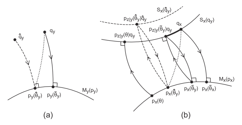
Figure 1: (a) Space of incomplete-data probability distributions. Projection from $q_{y}$ to the model manifold $M_{y}(p_{y})$ (arrow with a solid line), and that from $\hat{q}_{y}$ (arrow with a broken line) using eqs. (2) and (3) in Section 2, respectively. The dotted line indicates $D_{y}(q_{y};p_{y}(\bm{\hat{\theta}}_{y}))$, which is the loss function for ${\rm risk}_{y;y}$. (b) Space of complete-data probability distributions. Projection from $q_{x}$ to the model manifold $M_{x}(p_{x})$ using eq. (5) in Section 3.1. Projection from $p_{x}(\bm{\theta})$ to the data manifold $S_{x}(q_{y})$ using eq. (9) in Section 3.2. Alternating projections between the two manifolds using eq. (10) in Section 3.3. The dotted line indicates $D_{x}(q_{x};p_{x}(\bm{\hat{\theta}}_{y}))$, which is the loss function for ${\rm risk}_{x;y}$. The bold segment indicates $D_{x}(q_{x};p_{z|y}(\bm{\bar{\theta}}_{y})q_{y})$, which is assumed to be zero in (15).

3 Complete-data divergence

Here we review Kullback-Leibler divergence for complete data when only incomplete data can be observed (Csiszár and Tusnády, 1984; Amari, 1995).

3.1 Projection to the model manifold

Let $g_{x}$ and $f_{x}$ be the arbitrary probability distributions of complete data. The complete-data Kullback-Leibler divergence from $g_{x}$ to $f_{x}$ is

$$D_{x}(g_{x};f_{x})=-\int g_{x}(\bm{x})(\log f_{x}(\bm{x})-\log g_{x}(\bm{x}))\,d\bm{x}.$$

All the arguments of incomplete data in Section 2 apply to complete data by replacing $\bm{y}$ with $\bm{x}$ in the notation. For example, we write $D_{x}(g_{x};f_{x})=L_{x}(g_{x};f_{x})-L_{x}(g_{x})$ with $L_{x}(g_{x};f_{x})=-\int g_{x}(\bm{x})\log f_{x}(\bm{x})\,d\bm{x}$ and $L_{x}(g_{x})=L_{x}(g_{x};g_{x})$. The projection of $q_{x}$ to the model manifold $M_{x}(p_{x})=\{p_{x}(\bm{\theta}):\forall\bm{\theta}\in\Theta\}$ is defined as

$$\min_{f_{x}\in M_{x}(p_{x})}D_{x}(q_{x};f_{x})=D_{x}(q_{x};p_{x}(\bm{\bar{\theta}}_{x}))$$ (5)

with $\bm{\bar{\theta}}_{x}={\rm arg}\mathop{\rm min\,}\limits_{\bm{\theta}}L_{x}(q_{x};p_{x}(\bm{\theta}))$. Figure 1 (b) shows a geometric illustration. Note that $\bm{\bar{\theta}}_{x}\neq\bm{\bar{\theta}}_{y}$ and $p_{x}(\bm{\bar{\theta}}_{x})\neq p_{x}(\bm{\bar{\theta}}_{y})$ in general.

3.2 Projection to the data manifold

The following simple lemma helps understand how the incomplete-data divergence and the complete-data divergence are related.

Lemma 1.

For two distributions $g_{x}(\bm{x})$ and $f_{x}(\bm{x})$, we have

$$D_{x}(g_{x};f_{x})=D_{x}(g_{x};f_{z|y}g_{y})+D_{y}(g_{y};f_{y}),$$ (6)

where $f_{z|y}g_{y}$ represents the distribution $f_{z|y}(\bm{z}|\bm{y})g_{y}(\bm{y})$. Therefore, the difference of the two divergences is $D_{x}(g_{x};f_{x})-D_{y}(g_{y};f_{y})=D_{x}(g_{x};f_{z|y}g_{y})$, which is zero if $g_{z|y}=f_{z|y}$. For an arbitrary distribution $h_{x}(\bm{x})$, the last term in (6) is expressed as

$$D_{y}(g_{y};f_{y})=D_{x}(h_{z|y}g_{y};h_{z|y}f_{y}).$$ (7)

In particular, choosing $h_{x}=f_{x}$ gives $D_{y}(g_{y};f_{y})=D_{x}(f_{z|y}g_{y};f_{x})$, and

$$D_{x}(g_{x};f_{x})=D_{x}(g_{x};f_{z|y}g_{y})+D_{x}(f_{z|y}g_{y};f_{x}).$$ (8)

We consider the set of all probability distributions $g_{x}$ with the same marginal distribution $g_{y}=q_{y}$ for a specified $q_{y}$. This set is denoted as $S_{x}(q_{y})=\{g_{z|y}q_{y}:\forall g_{z|y}\}$. Note that the elements of $S_{x}(q_{y})$ are written as $g_{z|y}q_{y}$ with arbitrary $g_{z|y}$ because $\int g_{z|y}(\bm{z}|\bm{y})q_{y}(\bm{y})\,d\bm{z}=q_{y}(\bm{y})$. Equations (88) and (57) in Amari (1995) are $S_{x}(\hat{q}_{y})$ and its restriction to a finite dimensional model, respectively, and are called the observed data (sub)manifold there. Here, we call $S_{x}(q_{y})$ the expected data manifold and $S_{x}(\hat{q}_{y})$ the observed data manifold, although it may be abuse of the word “manifold” for subsets with infinite dimensions.

The projection of $p_{x}(\bm{\theta})$ to $S_{x}(q_{y})$ should be defined to minimize the complete-data divergence over $S_{x}(q_{y})$, but the roles of $g_{x}$ and $f_{x}$ in $D_{x}(g_{x};f_{x})$ are exchanged from those of (5). We minimize $D_{x}(g_{x};p_{x}(\bm{\theta}))$ over $g_{x}\in S_{x}(q_{y})$. By letting $g_{x}\in S_{x}(q_{y})$ and $f_{x}=p_{x}(\bm{\theta})$ in (6),

$$D_{x}(g_{x};p_{x}(\bm{\theta}))=D_{x}(g_{z|y}q_{y};p_{z|y}(\bm{\theta})q_{y})+D_{y}(q_{y};p_{y}(\bm{\theta})),$$

which is minimized when $g_{z|y}=p_{z|y}(\bm{\theta})$. Therefore, the projection gives the minimum value as

$$\min_{g_{x}\in S_{x}(q_{y})}D_{x}(g_{x};p_{x}(\bm{\theta}))=D_{y}(q_{y};p_{y}(\bm{\theta})).$$ (9)

Using (8), the minimum value can also be written as $D_{y}(q_{y};p_{y}(\bm{\theta}))=D_{x}(p_{z|y}(\bm{\theta})q_{y};p_{x}(\bm{\theta}))$.

3.3 Alternating projections between the two manifolds

The optimal parameter $\bm{\bar{\theta}}_{y}$ of the incomplete data is interpreted as a dual or alternate minimization problem of complete-data divergence. By minimizing (9) over $\bm{\theta}\in\Theta$, we define the alternating projections between $S_{x}(q_{y})$ and $M_{x}(p_{x})$ as

$$\min_{f_{x}\in M_{x}(p_{x})}\min_{g_{x}\in S_{x}(q_{y})}D_{x}(g_{x};f_{x})=D_{y}(q_{y};p_{y}(\bm{\bar{\theta}}_{y})),$$ (10)

where the minimum is attained by $g_{x}=p_{z|y}(\bm{\bar{\theta}}_{y})q_{y}$ and $f_{x}=p_{x}(\bm{\bar{\theta}}_{y})$. See eq. (65) in Amari (1995). This implies that $p_{z|y}(\bm{\bar{\theta}}_{y})q_{y}$ is the best approximation of $q_{x}$ when the two manifolds $S_{x}(q_{y})$ and $M_{x}(p_{x})$ are known, while $p_{x}(\bm{\bar{\theta}}_{y})$ is the best approximation of $q_{x}$ in $M_{x}(p_{x})$. This interpretation is the key to understanding our problem.

The above mentioned geometrical interpretation corresponds to the well known fact that the EM algorithm of Dempster, Laird and Rubin (1977) is alternating projections between $S_{x}(\hat{q}_{y})$ and $M_{x}(p_{x})$. See Csiszár and Tusnády (1984), Byrne (1992), Amari (1995), and Ip and Lalwani (2000). Starting from the initial value $\bm{\theta}^{(1)}$, the EM algorithm computes a sequence of the parameter values $\{\bm{\theta}^{(s)};s=1,2,\ldots\}$ by the updating formula $\bm{\theta}^{(s+1)}={\rm arg}\mathop{\rm max\,}\limits_{\bm{\theta}\in\Theta}Q(\bm{\theta};\bm{\theta}^{(s)})$. It follows from $L_{x}(p_{z|y}(\bm{\theta}_{1})\hat{q}_{y};p_{x}(\bm{\theta}_{2}))=-Q(\bm{\theta}_{2};\bm{\theta}_{1})/n$ that

$$\bm{\theta}^{(s+1)}={\rm arg}\mathop{\rm min\,}\limits_{\bm{\theta}\in\Theta}L_{x}(p_{z|y}(\bm{\theta}^{(s)})\hat{q}_{y};p_{x}(\bm{\theta})),$$

meaning $p_{x}(\bm{\theta}^{(s+1)})$ is the projection from $p_{z|y}(\bm{\theta}^{(s)})\hat{q}_{y}$ to $M_{x}(p_{x})$. Alternatively, $p_{z|y}(\bm{\theta}^{(s)})\hat{q}_{y}$ is the projection from $p_{x}(\bm{\theta}^{(s)})$ to $S_{x}(\hat{q}_{y})$. Thus, the converging point of the alternating projections satisfies

$$\bm{\hat{\theta}}_{y}={\rm arg}\mathop{\rm min\,}\limits_{\bm{\theta}\in\Theta}L_{x}(p_{z|y}(\bm{\hat{\theta}}_{y})\hat{q}_{y};p_{x}(\bm{\theta})).$$ (11)

4 Risk functions for model selection

By looking at the incomplete-data distributions, the discrepancy between the true distribution $q_{y}$ and our estimation $p_{y}(\bm{\hat{\theta}}_{y})$ is measured by the incomplete-data divergence $D_{y}(q_{y};p_{y}(\bm{\hat{\theta}}_{y}))$. If we take it as the loss function, the expected loss-function, or the risk function, will measure the discrepancy in the long run. Then AIC and its variants are derived as estimators of

$${\rm risk}_{y;y}=E\{D_{y}(q_{y};p_{y}(\bm{\hat{\theta}}_{y}))\}.$$ (12)

The expectation is evaluated with respect to $q_{x}$, although it involves only $q_{y}$ here. This is the standard approach in the literature (Akaike, 1974; Bozdogan, 1987; Burnham and Anderson, 2002; Konishi and Kitagawa, 2008).

Shimodaira (1994) and Cavanaugh and Shumway (1998) proposed another approach, which employs the complete-data divergence $D_{x}(q_{x};p_{x}(\bm{\hat{\theta}}_{y}))$ to measure the discrepancy between the complete-data distributions $q_{x}$ and $p_{x}(\bm{\hat{\theta}}_{y})$. Using the complete-data divergence as the loss function, the risk function becomes

$${\rm risk}_{x;y}=E\{D_{x}(q_{x};p_{x}(\bm{\hat{\theta}}_{y}))\}.$$ (13)

The first suffix $\bm{x}$ indicates the random variable for the loss function, while the second suffix $\bm{y}$ indicates the random variable for the observation.

However, estimating (13) is difficult. The complete-data empirical distribution $\hat{q}_{x}(\bm{x})=\frac{1}{n}\sum_{t=1}^{n}\delta(\bm{x}-\bm{x}_{t})$ is unknown; we only know that $\hat{q}_{x}$ is somewhere in the observed data manifold $S_{x}(\hat{q}_{y})$. Considering the limiting situation of $n\to\infty$, we may only know that the true distribution is somewhere in the expected data manifold: $q_{x}\in S_{x}(q_{y})$. Then the best substitute for $q_{x}$ is

$$q_{x}=p_{z|y}(\bm{\bar{\theta}}_{y})q_{y}$$ (14)

as suggested by (10) from the viewpoint of the alternating projections in Section 3.3. To estimate (13), we assume that (14) holds in this paper. This assumption is rephrased as

$$D_{x}(q_{x};p_{z|y}(\bm{\bar{\theta}}_{y})q_{y})=0$$

or equivalently

$$q_{z|y}=p_{z|y}(\bm{\bar{\theta}}_{y}),$$ (15)

implying that $p_{z|y}(\bm{\theta})$ is correctly specified for $q_{z|y}$ and that $\bm{\bar{\theta}}_{x}=\bm{\bar{\theta}}_{y}$, because the two projections from $q_{x}$ and $p_{z|y}(\bm{\bar{\theta}}_{y})q_{y}$ to $M_{x}(p_{x})$ become identical as illustrated in Fig. 1 (b). Because it is impossible to know how much $q_{z|y}$ actually deviates from $p_{z|y}(\bm{\bar{\theta}}_{y})$ when $Z=(\bm{z}_{1},\ldots,\bm{z}_{n})$ is missing completely, we assume (15) in the following argument to derive ${\rm AIC}_{x;y}$. Note that assumption (15) holds with $\bm{\bar{\theta}}_{x}=\bm{\bar{\theta}}_{y}=\bm{\theta}_{0}$ in the case of the correct specification where $q_{x}=p_{x}(\bm{\theta}_{0})$.

We are now ready to derive ${\rm AIC}_{x;y}$ as an estimator of $2n\,{\rm risk}_{x;y}$. The arguments in Lemma 2 and Theorem 1 almost duplicate that used to derive TIC mentioned in Burnham and Anderson (2002) and Konishi and Kitagawa (2008). However, it should be noted that in Lemma 2 the first term of ${\rm risk}_{x;y}$ is expressed by the incomplete-data divergence instead of the complete-data divergence. A point for proving the lemma is that

$$D_{x}(q_{x};p_{x}(\bm{\bar{\theta}}_{y}))=D_{x}(q_{x};p_{z|y}(\bm{\bar{\theta}}_{y})q_{y})+D_{y}(q_{y};p_{y}(\bm{\bar{\theta}}_{y}))=D_{y}(q_{y};p_{y}(\bm{\bar{\theta}}_{y})),$$ (16)

which follows from Lemma 1 and the assumption (15). $D_{x}(q_{x};p_{x}(\bm{\bar{\theta}}_{y}))$ on the left-hand side is the amount of misspecification of $p_{x}(\bm{\theta})$, and can be decomposed into the two parts: $D_{x}(q_{x};p_{z|y}(\bm{\bar{\theta}}_{y})q_{y})$ and $D_{y}(q_{y};p_{y}(\bm{\bar{\theta}}_{y}))$, which are the contribution of $p_{z|y}(\bm{\theta})$ and $p_{y}(\bm{\theta})$, respectively. To estimate (13), instead of estimating $D_{x}(q_{x};p_{z|y}(\bm{\bar{\theta}}_{y})q_{y})$, we ignore it.

Lemma 2.

Assume the regularity conditions of White (1982) mentioned in Section 2, and also assume that (15) holds. Then the expected loss is asymptotically expanded as

$${\rm risk}_{x;y}=D_{y}(q_{y};p_{y}(\bm{\bar{\theta}}_{y}))+\frac{1}{2n}\mathop{\rm tr}\nolimits(H_{x}H_{y}^{-1}G_{y}H_{y}^{-1})+O(n^{-3/2}).$$ (17)

The matrices $G_{y}$ and $H_{y}$ are those defined in Section 2, and $H_{x}=H_{x}(p_{z|y}(\bm{\bar{\theta}}_{y})q_{y};\bm{\bar{\theta}}_{y})$ with

$$H_{x}(g_{x};\bm{\theta})=-\int g_{x}(\bm{x})\frac{\partial^{2}\log p_{x}(\bm{x};\bm{\theta})}{\partial\bm{\theta}\partial\bm{\theta}^{T}}\,d\bm{x}.$$

The dominant term in (17) is also expressed as $D_{y}(q_{y};p_{y}(\bm{\bar{\theta}}_{y}))=L_{y}(q_{y};p_{y}(\bm{\bar{\theta}}_{y}))-L_{y}(q_{y})$ using the cross-entropy.

5 Information criteria

Let us define an information criterion as an estimator of ${\rm risk}_{x;y}$.

$$\widehat{\rm risk}_{x;y}=L_{y}(\hat{q}_{y};p_{y}(\bm{\hat{\theta}}_{y}))-L_{y}(q_{y})+\frac{1}{2n}\mathop{\rm tr}\nolimits(G_{y}H_{y}^{-1})+\frac{1}{2n}\mathop{\rm tr}\nolimits(H_{x}H_{y}^{-1}G_{y}H_{y}^{-1}),$$ (18)

where the matrices $G_{y}$, $H_{y}$ and $H_{x}$ may be replaced by their consistent estimators with error $O_{p}(n^{-1/2})$. When $\bm{x}\equiv\bm{y}$, (18) reduces to

$$\widehat{\rm risk}_{y;y}=L_{y}(\hat{q}_{y};p_{y}(\bm{\hat{\theta}}_{y}))-L_{y}(q_{y})+\frac{1}{n}\mathop{\rm tr}\nolimits(G_{y}H_{y}^{-1}),$$ (19)

which corresponds to the Takeuchi information criterion (TIC) for estimating ${\rm risk}_{y;y}$ mentioned in Burnham and Anderson (2002) and Konishi and Kitagawa (2008). In model selection, we ignore $L_{y}(q_{y})$, because all candidate models have the same value. The first term $L_{y}(\hat{q}_{y};p_{y}(\bm{\hat{\theta}}_{y}))=-\ell_{y}(\bm{\hat{\theta}}_{y})/n$ of order $O_{p}(1)$ measures the goodness of fit, while the last two terms of order $O(n^{-1})$ are interpreted as the penalty of model complexity. Our estimator is justified by the following theorem.

Theorem 1.

Assume the regularity conditions of White (1982) mentioned in Section 2, and also assume that (15) holds. Then we have

$$L_{y}(q_{y};p_{y}(\bm{\bar{\theta}}_{y}))=E\{L_{y}(\hat{q}_{y};p_{y}(\bm{\hat{\theta}}_{y}))\}+\frac{1}{2n}\mathop{\rm tr}\nolimits(G_{y}H_{y}^{-1})+O(n^{-3/2}),$$ (20)

and therefore

$$E\{\widehat{\rm risk}_{x;y}\}={\rm risk}_{x;y}+O(n^{-3/2}).$$ (21)

Thus, the estimator is unbiased asymptotically up to terms of order $O(n^{-1})$.

In the case of the correct specification where $q_{y}=p_{y}(\bm{\bar{\theta}}_{y})$ for the incomplete-data distribution, we have $G_{y}=H_{y}=I_{y}(\bm{\bar{\theta}}_{y})$, and the information matrix is consistently estimated by $I_{y}(\bm{\hat{\theta}}_{y})$. Assuming (15), this implies that $q_{x}=p_{x}(\bm{\bar{\theta}}_{x})$ is correctly specified for the complete-data distribution. Hence, $H_{x}=I_{x}(\bm{\bar{\theta}}_{y})$ is consistently estimated by $I_{x}(\bm{\hat{\theta}}_{y})$. For model selection, we assume that $p_{y}(\bm{\theta})$ is misspecified for $q_{y}$ in general. However, these equations may approximately hold if $p_{y}(\bm{\bar{\theta}}_{y})$ is a good approximation of $q_{y}$. By substituting $G_{y}\approx H_{y}\approx I_{y}(\bm{\bar{\theta}}_{y})$ and $H_{x}\approx I_{x}(\bm{\bar{\theta}}_{y})$ into (18) and (19), we have

$$\widehat{\rm risk}_{x;y}\approx L_{y}(\hat{q}_{y};p_{y}(\bm{\hat{\theta}}_{y}))-L_{y}(q_{y})+\frac{d}{2n}+\frac{1}{2n}\mathop{\rm tr}\nolimits(I_{x}(\bm{\hat{\theta}}_{y})I_{y}(\bm{\hat{\theta}}_{y})^{-1}),$$

and

$$\widehat{\rm risk}_{y;y}\approx L_{y}(\hat{q}_{y};p_{y}(\bm{\hat{\theta}}_{y}))-L_{y}(q_{y})+\frac{d}{n},$$

where $L_{y}(q_{y})$ is ignored for model selection. Multiplying by $2n$ converts these approximations to ${\rm AIC}_{x;y}$ and AIC, respectively.

6 PDIO and AICcd

The idea behind the derivation of PDIO and ${\rm AIC}_{cd}$ is to replace $\hat{q}_{x}$ by

$$\hat{q}_{x}=p_{z|y}(\bm{\hat{\theta}}_{y})\hat{q}_{y}.$$ (22)

This implies (14) by considering the limiting situation of $n\to\infty$. Thus, the assumption for PDIO and ${\rm AIC}_{cd}$ is stronger than the assumption for ${\rm AIC}_{x;y}$. Substituting (22) into the complete-data MLE gives

$$\bm{\hat{\theta}}_{x}={\rm arg}\mathop{\rm min\,}\limits_{\bm{\theta}\in\Theta}L_{x}(\hat{q}_{x};p_{x}(\bm{\theta})).$$ (23)

Comparing (23) with (11) gives $\bm{\hat{\theta}}_{x}=\bm{\hat{\theta}}_{y}$. Therefore, there should not be any missing data, or at least $p_{z|y}(\bm{\theta})$ should not involve the parameter $\bm{\theta}$. Consequently, AIC, PDIO, ${\rm AIC}_{cd}$, and ${\rm AIC}_{x;y}$ are equivalent when PDIO and ${\rm AIC}_{cd}$ are justified under (22).

Although assumption (22) is too strong to work with, it is interesting to see how PDIO and ${\rm AIC}_{cd}$ would be derived if (22) is formally accepted. The argument below to derive PDIO and ${\rm AIC}_{cd}$ is rather confusing because $\hat{q}_{x}$ is interpreted interchangeably as the complete-data empirical distribution or the right-hand side of (22).

By a similar argument to the proof of Theorem 1, the Taylor expansion of $L_{x}(\hat{q}_{x};p_{x}(\bm{\theta}))$ around $\bm{\theta}=\bm{\hat{\theta}}_{y}$ is

$$L_{x}(\hat{q}_{x};p_{x}(\bm{\theta}))=L_{x}(\hat{q}_{x};p_{x}(\bm{\hat{\theta}}_{y}))+\frac{1}{2}(\bm{\theta}-\bm{\hat{\theta}}_{y})^{T}\hat{H}_{x}(\bm{\theta}-\bm{\hat{\theta}}_{y})+O_{p}(n^{-3/2})$$ (24)

with $\hat{H}_{x}=H_{x}(\hat{q}_{x};\bm{\hat{\theta}}_{y})$. Its expectation with $\bm{\theta}=\bm{\bar{\theta}}_{y}$ gives

$$L_{x}(q_{x};p_{x}(\bm{\bar{\theta}}_{y}))=E\{L_{x}(\hat{q}_{x};p_{x}(\bm{\hat{\theta}}_{y}))\}+\frac{1}{2n}\mathop{\rm tr}\nolimits(H_{x}H_{y}^{-1}G_{y}H_{y}^{-1})+O(n^{-3/2}).$$ (25)

This corresponds to (20) of Theorem 1. Noticing (16) and thus, $D_{y}(q_{y};p_{y}(\bm{\bar{\theta}}_{y}))=L_{x}(q_{x};p_{x}(\bm{\bar{\theta}}_{y}))-L_{x}(q_{x})$, and then substituting (25) into (17) gives the estimator of ${\rm risk}_{x;y}$ unbiased up to $O(n^{-1})$ under (22) as

$$\widehat{\rm risk}_{x;y}=L_{x}(\hat{q}_{x};p_{x}(\bm{\hat{\theta}}_{y}))-L_{x}(q_{x})+\frac{1}{n}\mathop{\rm tr}\nolimits(H_{x}H_{y}^{-1}G_{y}H_{y}^{-1}).$$ (26)

The goodness of fit term is $L_{x}(p_{z|y}(\bm{\hat{\theta}}_{y})\hat{q}_{y};p_{x}(\bm{\hat{\theta}}_{y}))=-Q(\bm{\hat{\theta}}_{y};\bm{\hat{\theta}}_{y})/n$ under (22). Therefore, (26) gives ${\rm AIC}_{cd}$ by the same approximation used to derive ${\rm AIC}_{x;y}$.

In Cavanaugh and Shumway (1998), for evaluating (3.15) there, they assumed that $E\{Q(\bm{\theta}_{0};\bm{\hat{\theta}}_{y})\}\approx E\{Q(\bm{\theta}_{0};\bm{\theta}_{0})\}$ or $E(L_{x}(p_{z|y}(\bm{\hat{\theta}}_{y})\hat{q}_{y};p_{x}(\bm{\theta}_{0})))\approx L_{x}(p_{z|y}(\bm{\theta}_{0})q_{y};p_{x}(\bm{\theta}_{0}))$ under the correct specification $q_{x}=p_{x}(\bm{\theta}_{0})$. The equality holds exactly under (22) because $E(L_{x}(\hat{q}_{x};p_{x}(\bm{\theta}_{0})))=L_{x}(q_{x};p_{x}(\bm{\theta}_{0}))$ if $\hat{q}_{x}$ is interpreted as the empirical distribution. Unfortunately, the difference is $E\{Q(\bm{\theta}_{0};\bm{\hat{\theta}}_{y})\}-E\{Q(\bm{\theta}_{0};\bm{\theta}_{0})\}=O(1)$ in general without assuming (22), leading to the bias of ${\rm AIC}_{cd}$ even when (15) holds.

In Shimodaira (1994), (3.5) corresponds to our (24), where $\bm{\hat{\theta}}_{x}=\bm{\hat{\theta}}_{y}$ is assumed implicitly in order to ignore the first derivative. Although $L_{x}(\hat{q}_{x})$ diverges for continuous random variable $\bm{x}$, $D_{x}(\hat{q}_{x};p_{x}(\bm{\hat{\theta}}_{y}))=L_{x}(\hat{q}_{x};p_{x}(\bm{\hat{\theta}}_{y}))-L_{x}(\hat{q}_{x})$ is formally considered. Similar to (16), we then have $D_{x}(\hat{q}_{x};p_{x}(\bm{\hat{\theta}}_{y}))=D_{y}(\hat{q}_{y};p_{y}(\bm{\hat{\theta}}_{y}))$ in (3.6) there. From this argument, the goodness of fit term of (26) is $L_{x}(\hat{q}_{x};p_{x}(\bm{\hat{\theta}}_{y}))=L_{y}(\hat{q}_{y};p_{y}(\bm{\hat{\theta}}_{y}))+L_{x}(\hat{q}_{x})-L_{y}(\hat{q}_{y})$, where $L_{x}(\hat{q}_{x})-L_{y}(\hat{q}_{y})$ is independent of the model specification if $\hat{q}_{x}$ is interpreted as the empirical distribution. Therefore, (26) gives PDIO because $L_{x}(\hat{q}_{x};p_{x}(\bm{\hat{\theta}}_{y}))$ can be replaced with $L_{y}(\hat{q}_{y};p_{y}(\bm{\hat{\theta}}_{y}))$ for model selection.

7 Simulation study

7.1 Simulation 1

To verify Theorem 1, we performed a simulation study of the two-component normal mixture model defined as follows. Let $z\in\{1,2\}$ be a discrete random variable for the component label, and $y\in\mathbb{R}$ be a continuous random variable for the observation. The distribution of $z$ is $P(z=i)=\pi_{i}$ and the conditional distribution of $y$ given $z=i$ is the normal distribution with mean $\mu_{i}$ and variance $\sigma_{i}^{2}$. The true parameter for data generation is specified as $\bm{\theta}_{0}^{T}=(\pi_{1},\mu_{1},\mu_{2},\sigma_{1}^{2},\sigma_{2}^{2})=(0.6,-1,1,0.7^{2},0.7^{2})$. We consider two candidate models for selection. Model 1 is a two-component normal mixture model with a constraint $\sigma_{1}^{2}=\sigma_{2}^{2}$ ($d=4$), whereas Model 2 is the same model without the constraint ($d=5$). Because these two models are correctly specified, (15) holds. However, (22) obviously does not.

We generated $B=4000$ datasets with sample size $n=100,200,500,1000,2000,5000,10000$. They are denoted as $X^{(b)}=(\bm{x}^{(b)}_{1},\ldots,\bm{x}^{(b)}_{n})$, $b=1,\ldots,B$. We also generated datasets of sample size $\tilde{n}=15000$, which are denoted as $\tilde{X}^{(b)}=(\bm{\tilde{x}}^{(b)}_{1},\ldots,\bm{\tilde{x}}^{(b)}_{\tilde{n}})$ for computing the loss functions. For each $X^{(b)}=(Y^{(b)},Z^{(b)})$ and Model $k$, $k=1,2$, we computed the information criteria ${\rm AIC}(Y^{(b)},k)$, ${\rm PDIO}(Y^{(b)},k)$, ${\rm AIC}_{cd}(Y^{(b)},k)$, ${\rm AIC}_{x;y}(Y^{(b)},k)$, and the loss functions ${\rm loss}_{y;y}(Y^{(b)},k)=L_{y}(q_{y};p_{y}(\bm{\hat{\theta}}^{(b)}_{y}))$, ${\rm loss}_{x;y}(X^{(b)},k)=L_{x}(q_{x};p_{x}(\bm{\hat{\theta}}^{(b)}_{y}))$, where $\bm{\hat{\theta}}^{(b)}_{y}$ is computed from $Y^{(b)}$. In the formulas below, $:\approx$ denotes that the expectation on the left-hand side is computed numerically by the simulation on the right-hand side. The loss functions are computed numerically by

$${\rm loss}_{y;y}(Y^{(b)},k) :\approx-\frac{1}{\tilde{n}}\sum_{t=1}^{\tilde{n}}\log p_{y}(\bm{\tilde{y}}^{(b)}_{t};\bm{\hat{\theta}}^{(b)}_{y}),$$

$${\rm loss}_{x;y}(X^{(b)},k) :\approx-\frac{1}{\tilde{n}}\sum_{t=1}^{\tilde{n}}\log p_{x}(\bm{\tilde{x}}^{(b)}_{t};\bm{\hat{\theta}}^{(b)}_{y}),$$

where $p_{x}$, $p_{y}$, and $\bm{\hat{\theta}}^{(b)}_{y}$ are for Model $k$. Then the expectation with respect to $q_{x}=p_{x}(\bm{\theta}_{0})$ is computed by the simulation average. For example,

$$E(\Delta{\rm AIC}):\approx\frac{1}{B}\sum_{b=1}^{B}({\rm AIC}(Y^{(b)},1)-{\rm AIC}(Y^{(b)},2)),$$

$$\Delta{\rm risk}_{x;y}:\approx\frac{1}{B}\sum_{b=1}^{B}({\rm loss}_{x;y}(X^{(b)},1)-{\rm loss}_{x;y}(X^{(b)},2)).$$

This Monte Carlo method calculates the expectation accurately for sufficiently large $\tilde{n}$ and $B$.

The result shown in Table 1 verifies Theorem 1. For sufficiently large $n$, $E(\Delta{\rm AIC})=2n\Delta{\rm risk}_{y;y}$ and $E(\Delta{\rm AIC}_{x;y})=2n\Delta{\rm risk}_{x;y}$ hold very well. On the other hand, $E(\Delta{\rm PDIO})$ differs significantly from $2n\Delta{\rm risk}_{y;y}$ and $2n\Delta{\rm risk}_{x;y}$. Thus, PDIO is not a good estimator of either of these risk functions. In addition, the expected value of ${\rm AIC}_{cd}$ is similar to that of PDIO, but its variation is larger than PDIO, as seen in the standard errors.

Let us consider the difference ${\rm PDIO}-{\rm AIC}_{cd}$

$${\rm diff}(Y,\bm{\hat{\theta}}_{y})=2Q(\bm{\hat{\theta}}_{y};\bm{\hat{\theta}}_{y})-2\ell_{y}(\bm{\hat{\theta}}_{y})=2\sum_{t=1}^{n}\int p_{z|y}(\bm{z}|\bm{y}_{t};\bm{\hat{\theta}}_{y})\log p_{z|y}(\bm{z}|\bm{y}_{t};\bm{\hat{\theta}}_{y})\,d\bm{z},$$

and its difference between the two models, which is denoted as $\Delta{\rm diff}(Y,\bm{\hat{\theta}}_{y})=\Delta{\rm PDIO}-\Delta{\rm AIC}_{cd}$. $\Delta{\rm diff}(Y,\bm{\hat{\theta}}_{y})$ and $E(\Delta{\rm diff}(Y,\bm{\hat{\theta}}_{y}))$ can be very large, and they are $O(n)$ under model misspecification. If (15) holds, as is the case of Table 1, $E({\rm diff}(Y,\bm{\bar{\theta}}_{y}))=2n\int q_{x}(x)\log q_{z|y}(z|y)\,dx$ is independent of the model. Therefore, the difference becomes smaller; $\Delta{\rm diff}(Y,\bm{\hat{\theta}}_{y})=O_{p}(\sqrt{n})$ and $E(\Delta{\rm diff}(Y,\bm{\hat{\theta}}_{y}))=O(1)$.

Table 1: Expected values of the information criteria and the risk functions in Simulation 1. These values are differences between the two models with standard errors in parentheses.

$n$	100	200	500	1000	2000	5000	10000
$E(\Delta{\rm AIC})$	0.810	0.898	0.982	0.978	0.986	0.982	1.04
	(0.027)	(0.025)	(0.023)	(0.023)	(0.023)	(0.023)	(0.022)
$E(\Delta{\rm PDIO})$	43.5	41.1	37.0	36.0	34.9	34.4	34.2
	(1.64)	(0.716)	(0.344)	(0.220)	(0.141)	(0.088)	(0.064)
$E(\Delta{\rm AIC}_{cd})$	42.3	41.0	37.2	36.6	35.2	35.5	33.5
	(1.67)	(0.793)	(0.518)	(0.494)	(0.573)	(0.812)	(1.08)
$E(\Delta{\rm AIC}_{x;y})$	22.1	21.0	19.0	18.5	18.0	17.7	17.6
	(0.821)	(0.361)	(0.174)	(0.113)	(0.074)	(0.049)	(0.037)
$2n\Delta{\rm risk}_{y;y}$	1.83	1.47	1.15	1.08	1.03	1.02	0.967
	(0.052)	(0.040)	(0.030)	(0.027)	(0.026)	(0.030)	(0.033)
$2n\Delta{\rm risk}_{x;y}$	100.9	28.9	20.3	18.6	18.2	17.5	17.0
	(40.3)	(1.39)	(0.620)	(0.487)	(0.456)	(0.464)	(0.430)

7.2 Simulation 2

We next performed a simulation study on the three-component normal mixture model to examine how well the information criteria work for model selection in a practical situation where some candidate models do not satisfy assumption (15). The true parameter value is $\bm{\theta}_{0}^{T}=(\pi_{1},\pi_{2},\mu_{1},\mu_{2},\mu_{3},\sigma_{1}^{2},\sigma_{2}^{2},\sigma_{3}^{2})=(0.5,0.3,-2,0,3,0.7^{2},0.7^{2},1^{2})$. We consider five candidates with the following constraints. Model 1 is $\sigma_{1}^{2}=\sigma_{2}^{2}=\sigma_{3}^{2}$ ($d=6$). Model 2 is $\sigma_{2}^{2}=\sigma_{3}^{2}$ ($d=7$). Model 3 is $\sigma_{1}^{2}=\sigma_{3}^{2}$ ($d=7$). Model 4 is $\sigma_{1}^{2}=\sigma_{2}^{2}$ ($d=7$), and Model 5 has no constraint ($d=8$). Model 1, Model 2, and Model 3 are misspecified and do not satisfy (15). Model 4 and Model 5 are correctly specified and satisfy (15). None of the models satisfy (22). We have generated $B=10000$ datasets of $n=500$ and $\tilde{n}=2000$.

Table 2 shows the model selection results. Model 4 is the best model in the sense that it minimizes both ${\rm risk}_{y;y}$ and ${\rm risk}_{x;y}$ (Table 3). All the information criteria tend to select Model 4. AIC tends to choose a more complex model (i.e., Model 2 or Model 5) than the other criteria, indicating a smaller penalty for model complexity. PDIO tends to choose a simpler model (i.e., Model 1), implying a larger penalty for model complexity.

To compare candidate models in the long run, the expected loss of each Model $k$ relative to that of Model 4 is computed by

$$\Delta{\rm risk}_{x;y}(k):\approx\frac{1}{B}\sum_{b=1}^{B}({\rm loss}_{x;y}(X^{(b)},k)-{\rm loss}_{x;y}(X^{(b)},4)).$$

Table 3 (upper) shows the results. The most complex model (Model 5) is the second best in terms of ${\rm risk}_{y;y}$, but the simplest model (Model 1) is the second best in terms of ${\rm risk}_{x;y}$, indicating a large contribution of $p_{z|y}(\bm{\theta})$ to the second term of (17).

The information criterion performance is measured by the expected loss of the selected model. For example, the performance of AIC in terms of complete data is measured by

$$\Delta{\rm risk}_{x;y}({\rm AIC}):\approx\frac{1}{B}\sum_{b=1}^{B}({\rm loss}_{x;y}(X^{(b)},\hat{k}^{(b)})-{\rm loss}_{x;y}(X^{(b)},4)),$$

where $\hat{k}^{(b)}$ is the minimum AIC model computed from $Y^{(b)}$. Table 3 (lower) shows the results, where the value in bold denotes the minimum value of each column. AIC outperforms the other criteria in terms of ${\rm risk}_{y;y}$, and ${\rm AIC}_{x;y}$ outperforms the other criteria in terms of ${\rm risk}_{x;y}$. In this example, some models do not satisfy assumption (15), but AIC and ${\rm AIC}_{x;y}$ work very well as expected.

Table 2: Frequency of model selection in Simulation 2.

		Model 1	Model 2	Model 3	Model 4$*$	Model 5$*$
		($d=6$)	($d=7$)	($d=7$)	($d=7$)	($d=8$)
AIC		881	2419	262	5600	838
PDIO		5442	16	4	4534	4
${\rm AIC}_{cd}$		2063	2	974	6551	410
${\rm AIC}_{x;y}$		3704	65	15	6190	26

• correctly specified model

Table 3: Risk functions for models and those for information criteria in Simulation 2. These values are relative to Model 4 with standard errors in parentheses.

		$2n\Delta{\rm risk}_{y;y}$			$2n\Delta{\rm risk}_{x;y}$
Model 1		6.60	(0.04)		33.2	(0.21)
Model 2		1.40	(0.02)		59.2	(0.71)
Model 3		7.86	(0.04)		80.7	(0.80)
Model 4$*$		0	(0.00)		0	(0.00)
Model 5$*$		1.32	(0.02)		45.6	(0.87)
AIC		1.44	(0.03)		39.6	(0.91)
PDIO		3.57	(0.04)		19.6	(0.30)
${\rm AIC}_{cd}$		2.33	(0.04)		28.2	(0.72)
${\rm AIC}_{x;y}$		2.36	(0.04)		14.8	(0.43)

• correctly specified model

8 Concluding remarks

We derived ${\rm AIC}_{x;y}$ as an unbiased estimator of the expected Kullback-Leibler divergence between the true distribution and the estimated distribution of complete data when only incomplete data is available. In Simulation 1, ${\rm AIC}_{x;y}$ and AIC are unbiased up to the penalty terms, whereas PDIO and ${\rm AIC}_{cd}$ are not.

To derive ${\rm AIC}_{x;y}$, we assumed (15), meaning that the conditional distribution $p_{z|y}(\bm{\theta})$ of the missing data given the incomplete data is correctly specified, while the marginal distribution $p_{y}(\bm{\theta})$ of the incomplete data is misspecified in general. However, the conditional distribution is misspecified in practice. In Simulation 2, we observed that ${\rm AIC}_{x;y}$ and AIC perform better than the other criteria even if some models are misspecified. Without assumption (15), the dominant term in (17) is $D_{x}(q_{x};p_{x}(\bm{\bar{\theta}}_{y}))=D_{x}(q_{x};p_{z|y}(\bm{\bar{\theta}}_{y})q_{y})+D_{y}(q_{y};p_{y}(\bm{\bar{\theta}}_{y}))\geq D_{y}(q_{y};p_{y}(\bm{\bar{\theta}}_{y}))$. Thus, ${\rm AIC}_{x;y}$ estimates the lower bound of $2n\,{\rm risk}_{x;y}$. It is impossible to reasonably estimate the ignored term $D_{x}(q_{x};p_{z|y}(\bm{\bar{\theta}}_{y})q_{y})$ in our setting where $z_{1},\ldots,z_{n}$ are missing completely.

Although we assume that $p_{z|y}(\bm{\theta})$ is correctly specified, it is beneficial to include $p_{z|y}(\bm{\theta})$ as a part of $p_{x}(\bm{\theta})=p_{z|y}(\bm{\theta})p_{y}(\bm{\theta})$ for model selection. The variance of $\bm{\hat{\theta}}_{y}$ causes $p_{z|y}(\bm{\hat{\theta}}_{y})$ to fluctuate even if $p_{z|y}(\bm{\bar{\theta}}_{y})=q_{z|y}$. The amount of this random variation is measured by the additional penalty term (1) in ${\rm AIC}_{x;y}$.

In the future, we plan to work on more complicated missing mechanisms or combine a missing mechanism with other sampling mechanisms, such as the covariate-shift (Shimodaira, 2000) problem. One important extension is semi-supervised learning (Chapelle, Schölkopf and Zien, 2006; Kawakita and Takeuchi, 2014), where the log-likelihood function is

$$\ell(\bm{\theta})=\sum_{t=1}^{n}\log p_{y}(\bm{y}_{t};\bm{\theta})+\sum_{t={n+1}}^{n+n^{\prime}}\log p_{x}(\bm{x}_{t};\bm{\theta}).$$

In this case, the additional complete data $\bm{x}_{n+1},\ldots,\bm{x}_{n+n^{\prime}}$ helps estimate conditional distribution $q_{z|y}$. We may reasonably estimate $D_{x}(q_{x};p_{z|y}(\bm{\bar{\theta}}_{y})q_{y})$ without assuming (15), leading to a new information criterion, which will be the subject in future research.

Appendix A Technical details

A.1 Proof of Lemma 1

For brevity, we omit $(\bm{y},\bm{z})$ of $f_{x}(\bm{y},\bm{z})$ in the integrals below. $D_{x}(g_{x};f_{x})=\int\int g_{z|y}g_{y}(\log g_{z|y}+\log g_{y}-\log f_{z|y}-\log f_{y})d\bm{z}d\bm{y}=\int g_{y}\int g_{z|y}(\log g_{z|y}-\log f_{z|y})d\bm{z}d\bm{y}+\int g_{y}(\int g_{z|y}d\bm{z})(\log g_{y}-\log f_{y})d\bm{y}=\int g_{y}\int g_{z|y}(\log g_{z|y}g_{y}-\log f_{z|y}g_{y})d\bm{z}d\bm{y}+\int g_{y}(\log g_{y}-\log f_{y})d\bm{y}=D_{x}(g_{z|y}g_{y};f_{z|y}g_{y})+D_{y}(g_{y};f_{y})$, thus showing (6). $D_{y}(g_{y};f_{y})=\int\int h_{z|y}g_{y}(\log g_{y}-\log f_{y}+\log h_{z|y}-\log h_{z|y})d\bm{z}d\bm{y}=D_{x}(h_{z|y}g_{y};h_{z|y}f_{y})$, which shows (7).

A.2 Proof of Lemma 2

We assume $q_{z|y}=p_{z|y}(\bm{\bar{\theta}}_{y})$ and $\bm{\bar{\theta}}_{x}=\bm{\bar{\theta}}_{y}$. From the definitions of $\bm{\bar{\theta}}_{x}$ and $H_{x}$, we have

$$\frac{\partial D_{x}(q_{x};p_{x}(\bm{\theta}))}{\partial\bm{\theta}}\Bigr{|}_{\bm{\bar{\theta}}_{y}}=0,\quad\frac{\partial^{2}D_{x}(q_{x};p_{x}(\bm{\theta}))}{\partial\bm{\theta}\partial\bm{\theta}^{T}}\Bigr{|}_{\bm{\bar{\theta}}_{y}}=H_{x}.$$

Hence, the Taylor expansion of $D_{x}(q_{x};p_{x}(\bm{\theta}))$ around $\bm{\theta}=\bm{\bar{\theta}}_{y}$ is

$$D_{x}(q_{x};p_{x}(\bm{\theta}))=D_{x}(q_{x};p_{x}(\bm{\bar{\theta}}_{y}))+\frac{1}{2}(\bm{\theta}-\bm{\bar{\theta}}_{y})^{T}H_{x}(\bm{\theta}-\bm{\bar{\theta}}_{y})+O(n^{-3/2})$$

for $\bm{\theta}-\bm{\bar{\theta}}_{y}=O(n^{-1/2})$. The first term on the right-hand side is $D_{y}(q_{y};p_{y}(\bm{\bar{\theta}}_{y}))$ as shown in (16). Substituting $\bm{\theta}=\bm{\hat{\theta}}_{y}$ in $D_{x}(q_{x};p_{x}(\bm{\theta}))$ and taking its expectation gives (17) by noting

$$E\left\{(\bm{\hat{\theta}}_{y}-\bm{\bar{\theta}}_{y})^{T}H_{x}(\bm{\hat{\theta}}_{y}-\bm{\bar{\theta}}_{y})\right\}=\mathop{\rm tr}\nolimits\left(H_{x}\,E\left\{(\bm{\hat{\theta}}_{y}-\bm{\bar{\theta}}_{y})(\bm{\hat{\theta}}_{y}-\bm{\bar{\theta}}_{y})^{T}\right\}\right),$$

which becomes $\mathop{\rm tr}\nolimits\left(H_{x}H_{y}^{-1}G_{y}H_{y}^{-1}\right)/n+O(n^{-2})$ from (4).

A.3 Proof of Theorem 1

From the definitions of $\bm{\hat{\theta}}_{y}$ and $\hat{H}_{y}=H_{y}(\hat{q}_{y};\bm{\hat{\theta}}_{y})$, we have

$$\frac{\partial L_{y}(\hat{q}_{y};p_{y}(\bm{\theta}))}{\partial\bm{\theta}}\Bigr{|}_{\bm{\hat{\theta}}_{y}}=0,\quad\frac{\partial^{2}L_{y}(\hat{q}_{y};p_{y}(\bm{\theta}))}{\partial\bm{\theta}\partial\bm{\theta}^{T}}\Bigr{|}_{\bm{\hat{\theta}}_{y}}=\hat{H}_{y}.$$

Hence, the Taylor expansion of $L_{y}(\hat{q}_{y};p_{y}(\bm{\theta}))$ around $\bm{\theta}=\bm{\hat{\theta}}_{y}$ is

$$L_{y}(\hat{q}_{y};p_{y}(\bm{\theta}))=L_{y}(\hat{q}_{y};p_{y}(\bm{\hat{\theta}}_{y}))+\frac{1}{2}(\bm{\theta}-\bm{\hat{\theta}}_{y})^{T}\hat{H}_{y}(\bm{\theta}-\bm{\hat{\theta}}_{y})+O_{p}(n^{-3/2})$$

for $\bm{\theta}-\bm{\hat{\theta}}_{y}=O_{p}(n^{-1/2})$. Substituting $\bm{\theta}=\bm{\bar{\theta}}_{y}$ in $L_{y}(\hat{q}_{y};p_{y}(\bm{\theta}))$, we take its expectation below. By noting $\hat{H}_{y}=H_{y}+O_{p}(n^{-1/2})$, we have

$$E\left\{(\bm{\bar{\theta}}_{y}-\bm{\hat{\theta}}_{y})^{T}\hat{H}_{y}(\bm{\bar{\theta}}_{y}-\bm{\hat{\theta}}_{y})\right\}=\mathop{\rm tr}\nolimits\left(H_{y}\,E\left\{(\bm{\hat{\theta}}_{y}-\bm{\bar{\theta}}_{y})(\bm{\hat{\theta}}_{y}-\bm{\bar{\theta}}_{y})^{T}\right\}\right)+O(n^{-3/2}),$$

which becomes $\mathop{\rm tr}\nolimits(H_{y}H_{y}^{-1}G_{y}H_{y}^{-1})/n+O(n^{-3/2})$ from (4). This proves (20) because

$$E\{L_{y}(\hat{q}_{y};p_{y}(\bm{\bar{\theta}}_{y}))\}=E\{L_{y}(\hat{q}_{y};p_{y}(\bm{\hat{\theta}}_{y}))\}+\frac{1}{2n}\mathop{\rm tr}\nolimits(G_{y}H_{y}^{-1})+O(n^{-3/2}),$$

and $E\{L_{y}(\hat{q}_{y};p_{y}(\bm{\bar{\theta}}_{y}))\}=L_{y}(q_{y};p_{y}(\bm{\bar{\theta}}_{y}))$. Substituting (20) into (17) and comparing it with (18) yields (21).

References

- Akaike (1974) {barticle}[author] \bauthor\bsnmAkaike, \bfnmHirotugu\binitsH. (\byear1974). \btitleA new look at the statistical model identification. \bjournalAutomatic Control, IEEE Transactions on \bvolume19 \bpages716–723. \endbibitem
- Amari (1995) {barticle}[author] \bauthor\bsnmAmari, \bfnmShun-Ichi\binitsS.-I. (\byear1995). \btitleInformation geometry of the EM and em algorithms for neural networks. \bjournalNeural networks \bvolume8 \bpages1379–1408. \endbibitem
- Amari and Nagaoka (2007) {bbook}[author] \bauthor\bsnmAmari, \bfnmShun-Ichi\binitsS.-I. and \bauthor\bsnmNagaoka, \bfnmHiroshi\binitsH. (\byear2007). \btitleMethods of information geometry \bvolume191. \bpublisherAmerican Mathematical Soc. \endbibitem
- Bozdogan (1987) {barticle}[author] \bauthor\bsnmBozdogan, \bfnmHamparsum\binitsH. (\byear1987). \btitleModel selection and Akaike’s information criterion (AIC): The general theory and its analytical extensions. \bjournalPsychometrika \bvolume52 \bpages345–370. \endbibitem
- Burnham and Anderson (2002) {bbook}[author] \bauthor\bsnmBurnham, \bfnmKenneth P\binitsK. P. and \bauthor\bsnmAnderson, \bfnmDavid R\binitsD. R. (\byear2002). \btitleModel selection and multimodel inference: a practical information-theoretic approach. \bpublisherSpringer. \endbibitem
- Byrne (1992) {barticle}[author] \bauthor\bsnmByrne, \bfnmWilliam\binitsW. (\byear1992). \btitleAlternating minimization and Boltzmann machine learning. \bjournalNeural Networks, IEEE Transactions on \bvolume3 \bpages612–620. \endbibitem
- Cavanaugh and Shumway (1998) {barticle}[author] \bauthor\bsnmCavanaugh, \bfnmJoseph E\binitsJ. E. and \bauthor\bsnmShumway, \bfnmRobert H\binitsR. H. (\byear1998). \btitleAn Akaike information criterion for model selection in the presence of incomplete data. \bjournalJournal of statistical planning and inference \bvolume67 \bpages45–65. \endbibitem
- Chapelle, Schölkopf and Zien (2006) {bbook}[author] \bauthor\bsnmChapelle, \bfnmOlivier\binitsO., \bauthor\bsnmSchölkopf, \bfnmBernhard\binitsB. and \bauthor\bsnmZien, \bfnmAlexander\binitsA. (\byear2006). \btitleSemi-supervised learning. \bpublisherMIT Press. \endbibitem
- Claeskens and Consentino (2008) {barticle}[author] \bauthor\bsnmClaeskens, \bfnmGerda\binitsG. and \bauthor\bsnmConsentino, \bfnmFabrizio\binitsF. (\byear2008). \btitleVariable selection with incomplete covariate data. \bjournalBiometrics \bvolume64 \bpages1062–1069. \endbibitem
- Csiszár (1975) {barticle}[author] \bauthor\bsnmCsiszár, \bfnmImre\binitsI. (\byear1975). \btitleI-divergence geometry of probability distributions and minimization problems. \bjournalThe Annals of Probability \bvolume3 \bpages146–158. \endbibitem
- Csiszár and Tusnády (1984) {barticle}[author] \bauthor\bsnmCsiszár, \bfnmImre\binitsI. and \bauthor\bsnmTusnády, \bfnmGábor\binitsG. (\byear1984). \btitleInformation geometry and alternating minimization procedures. \bjournalStatistics and decisions, Supplement Issue \bvolume1 \bpages205–237. \endbibitem
- Dempster, Laird and Rubin (1977) {barticle}[author] \bauthor\bsnmDempster, \bfnmArthur P\binitsA. P., \bauthor\bsnmLaird, \bfnmNan M\binitsN. M. and \bauthor\bsnmRubin, \bfnmDonald B\binitsD. B. (\byear1977). \btitleMaximum likelihood from incomplete data via the EM algorithm. \bjournalJournal of the Royal Statistical Society. Series B (methodological) \bvolume39 \bpages1–38. \endbibitem
- Ip and Lalwani (2000) {barticle}[author] \bauthor\bsnmIp, \bfnmEdward H\binitsE. H. and \bauthor\bsnmLalwani, \bfnmNeal\binitsN. (\byear2000). \btitleA note on the geometric interpretation of the EM algorithm in estimating item characteristics and student abilities. \bjournalPsychometrika \bvolume65 \bpages533–537. \endbibitem
- Kawakita and Takeuchi (2014) {barticle}[author] \bauthor\bsnmKawakita, \bfnmMasanori\binitsM. and \bauthor\bsnmTakeuchi, \bfnmJun’ichi\binitsJ. (\byear2014). \btitleSafe semi-supervised learning based on weighted likelihood. \bjournalNeural Networks \bvolume53 \bpages146–164. \endbibitem
- Konishi and Kitagawa (2008) {bbook}[author] \bauthor\bsnmKonishi, \bfnmSadanori\binitsS. and \bauthor\bsnmKitagawa, \bfnmGenshiro\binitsG. (\byear2008). \btitleInformation criteria and statistical modeling. \bpublisherSpringer Science & Business Media. \endbibitem
- Meng and Rubin (1991) {barticle}[author] \bauthor\bsnmMeng, \bfnmXiao-Li\binitsX.-L. and \bauthor\bsnmRubin, \bfnmDonald B\binitsD. B. (\byear1991). \btitleUsing EM to obtain asymptotic variance-covariance matrices: The SEM algorithm. \bjournalJournal of the American Statistical Association \bvolume86 \bpages899–909. \endbibitem
- Seghouane, Bekara and Fleury (2005) {barticle}[author] \bauthor\bsnmSeghouane, \bfnmAbd-Krim\binitsA.-K., \bauthor\bsnmBekara, \bfnmMaiza\binitsM. and \bauthor\bsnmFleury, \bfnmGilles\binitsG. (\byear2005). \btitleA criterion for model selection in the presence of incomplete data based on Kullback’s symmetric divergence. \bjournalSignal processing \bvolume85 \bpages1405–1417. \endbibitem
- Shimodaira (1994) {bincollection}[author] \bauthor\bsnmShimodaira, \bfnmHidetoshi\binitsH. (\byear1994). \btitleA new criterion for selecting models from partially observed data. In \bbooktitleSelecting Models from Data \bpages21–29. \bpublisherSpringer-Verlag. \endbibitem
- Shimodaira (2000) {barticle}[author] \bauthor\bsnmShimodaira, \bfnmHidetoshi\binitsH. (\byear2000). \btitleImproving predictive inference under covariate shift by weighting the log-likelihood function. \bjournalJournal of Statistical Planning and Inference \bvolume90 \bpages227–244. \endbibitem
- White (1982) {barticle}[author] \bauthor\bsnmWhite, \bfnmHalbert\binitsH. (\byear1982). \btitleMaximum likelihood estimation of misspecified models. \bjournalEconometrica \bvolume50 \bpages1–25. \endbibitem
- Yamazaki (2014) {barticle}[author] \bauthor\bsnmYamazaki, \bfnmKeisuke\binitsK. (\byear2014). \btitleAsymptotic accuracy of distribution-based estimation of latent variables. \bjournalThe Journal of Machine Learning Research \bvolume15 \bpages3541–3562. \endbibitem