Model-Independent Measurement of the e${}^{\text{+}}$e${}^{\text{--}}$ $\to$ HZ Cross Section at a Future e${}^{\text{+}}$e${}^{\text{--}}$ Linear Collider using Hadronic Z Decays

Abstract

A future $\mathup{{{\mathup{{{e}}}}}^{\scriptstyle{+}}}\mathup{{{\mathup{{{e}}}}}^{\scriptstyle{-}}}$ collider, such as the ILC or CLIC, would allow the Higgs sector to be probed with a precision significantly beyond that achievable at the High-Luminosity LHC. A central part of the Higgs programme at an $\mathup{{{\mathup{{{e}}}}}^{\scriptstyle{+}}}\mathup{{{\mathup{{{e}}}}}^{\scriptstyle{-}}}$ collider is the model-independent determination of the absolute Higgs couplings to fermions and to gauge bosons. Here the measurement of the $\mathup{{{\mathup{{{e}}}}}^{\scriptstyle{+}}}\mathup{{{\mathup{{{e}}}}}^{\scriptstyle{-}}}\to\mathup{{{H}}}\mathup{{{Z}}}$ Higgsstrahlung cross section, using the recoil mass technique, sets the absolute scale for all Higgs coupling measurements. Previous studies have considered $\sigma(\mathup{{{\mathup{{{e}}}}}^{\scriptstyle{+}}}\mathup{{{\mathup{{{e}}}}}^{\scriptstyle{-}}}\to\mathup{{{H}}}\mathup{{{Z}}})$ with $\mathup{{{Z}}}\to\mathup{{{\ell}}^{\scriptstyle{+}}}\mathup{{{\ell}}^{\scriptstyle{-}}}$, where $\ell=\mathup{{{e}}},\,\mathup{}$. In this paper it is shown for the first time that a near model-independent recoil mass technique can be extended to the hadronic decays of the $\mathup{{{Z}}}$ boson. Because the branching ratio for $\mathup{{{Z}}}\to\mathup{{{q}}}\mathup{{\overline{{\mathup{{{q}}}}}}}$ is approximately ten times greater than for $\mathup{{{Z}}}\to\mathup{{{\ell}}^{\scriptstyle{+}}}\mathup{{{\ell}}^{\scriptstyle{-}}}$, this method is statistically more powerful than using the leptonic decays. For an integrated luminosity of 500 $\text{fb}^{-1}$ at a centre-of-mass energy of $\sqrt{s}=350\,\text{GeV}$ at CLIC, $\sigma(\mathup{{{\mathup{{{e}}}}}^{\scriptstyle{+}}}\mathup{{{\mathup{{{e}}}}}^{\scriptstyle{-}}}\to\mathup{{{H}}}\mathup{{{Z}}})$ can be measured to $\pm 1.8\,\%$ using the hadronic recoil mass technique. A similar precision is found for the ILC operating at $\sqrt{s}=350\,\text{GeV}$. The centre-of-mass dependence of this measurement technique is discussed, arguing for the initial operation of a future linear collider at just above the top-pair production threshold.

1 Introduction

A future $\mathup{{{\mathup{{{e}}}}}^{\scriptstyle{+}}}\mathup{{{\mathup{{{e}}}}}^{\scriptstyle{-}}}$ collider, such as the Compact Linear Collider (CLIC) bib:CLIC_CDR or the International Linear Collider (ILC) bib:ILC_TDR , would be complementary to the Large Hadron Collider (LHC) and the High-Luminosity LHC (HL-LHC), providing tests of beyond the Standard Model (SM) physics scenarios through a broad programme of highly precise measurements. A central part of the linear collider physics programme is the precise study of the properties of the Higgs boson. The LHC and HL-LHC will provide an impressive range of Higgs physics measurements, establishing the general properties of the Higgs boson, such as its mass and spin. The LHC will also provide measurements of the product of the Higgs production rate and Higgs decay branching fractions into different final states. Current estimates suggest that ratios of couplings can be measured to 2 % – 7 % (depending on the final state) with 3000 fb^-1 of data bib:SnowmassHiggs . A number of recent studies, see for example bib:SnowmassHiggs ; bib:Wells , have indicated that modifications of the Higgs couplings due to beyond the SM (BSM) physics are almost always less than 10 % and can be as small as 1 % – 2 % in a number of models.

An $\mathup{{{\mathup{{{e}}}}}^{\scriptstyle{+}}}\mathup{{{\mathup{{{e}}}}}^{\scriptstyle{-}}}$ collider would be a unique facility for precision Higgs physics bib:ILC_Physics_TDR ; bib:CLIC_Snowmass , providing measurements of the Higgs boson branching ratios that may be an order of magnitude more precise than those achievable at the HL-LHC. Such measurements may be necessary to reveal BSM effects in the Higgs sector. Moreover, an $\mathup{{{\mathup{{{e}}}}}^{\scriptstyle{+}}}\mathup{{{\mathup{{{e}}}}}^{\scriptstyle{-}}}$ collider provides the opportunity to make a number of unique measurements including: i) absolute measurements of Higgs couplings, rather than ratios; ii) a precise measurement of possible decays to invisible (long-lived neutral) final states; and iii) a $<10\,\%$ measurement of the total Higgs decay width, $\Gamma_{\mathup{{{H}}}}$. In addition, an $\mathup{{{\mathup{{{e}}}}}^{\scriptstyle{+}}}\mathup{{{\mathup{{{e}}}}}^{\scriptstyle{-}}}$ collider operating at 1 TeV or above, for example CLIC or an upgraded ILC, would have sensitivity to the Yukawa coupling of the top quark to the Higgs boson and the Higgs self-coupling parameter $\lambda$, thus providing a direct probe of the Higgs potential.

This paper presents the first detailed study of the potential of making a model-independent measurement of $g_{\mathup{{{H}}}\mathup{{{Z}}}\mathup{{{Z}}}}$ from the recoil mass distribution in $\mathup{{{\mathup{{{e}}}}}^{\scriptstyle{+}}}\mathup{{{\mathup{{{e}}}}}^{\scriptstyle{-}}}\to\mathup{{{H}}}\mathup{{{Z}}}$ with $\mathup{{{Z}}}\to\mathup{{{q}}}\mathup{{\overline{{\mathup{{{q}}}}}}}$, denoted as $\mathup{{{H}}}\mathup{{{Z}}}(\mathup{{{Z}}}\to\mathup{{{q}}}\mathup{{\overline{{\mathup{{{q}}}}}}})$. The studies were initially performed in the context of the CLIC accelerator operating at $\sqrt{s}=350\,\text{GeV}$. The studies were repeated for the ILC operating at the same energy and for CLIC at $\sqrt{s}=250\,\text{GeV}$ and $\sqrt{s}=420\,\text{GeV}$.

1.1 Higgs production in $e^{+}e^{-}$ collisions

In $\mathup{{{\mathup{{{e}}}}}^{\scriptstyle{+}}}\mathup{{{\mathup{{{e}}}}}^{\scriptstyle{-}}}$ collisions at $\sqrt{s}$ = 250 – 500 GeV, the two main Higgs production mechanisms are the Higgsstrahlung process, $\mathup{{{\mathup{{{e}}}}}^{\scriptstyle{+}}}\mathup{{{\mathup{{{e}}}}}^{\scriptstyle{-}}}\to\mathup{{{H}}}\mathup{{{Z}}}$, and the $\mathup{{{W}}}\mathup{{{W}}}$-fusion process, $\mathup{{{\mathup{{{e}}}}}^{\scriptstyle{+}}}\mathup{{{\mathup{{{e}}}}}^{\scriptstyle{-}}}\to\mathup{{{H}}}\mathup{{{\mathup{}}}{}_{\scriptstyle{\!\mathup{{{e}}}}}}\mathup{{\overline{{\mathup{}}}}{}_{\scriptstyle{\!\mathup{{{e}}}}}}$, shown in Fig. 1. For $m_{\mathup{{{H}}}}\sim 125\,$GeV, the cross section for the $s$-channel Higgsstrahlung process is maximal close to $\sqrt{s}=250\,\text{GeV}$, whereas the cross section for the $t$-channel $\mathup{{{W}}}\mathup{{{W}}}$-fusion process increases with centre-of-mass energy, as indicated in Tab. 1.

eezh (25,20) i1,i2 o1,o2 $\mathup{{{\mathup{{{e}}}}}^{\scriptstyle{-}}}$i1 $\mathup{{{\mathup{{{e}}}}}^{\scriptstyle{+}}}$i2 $\mathup{{{Z}}}$o2 $\mathup{{{H}}}$o1 photon,tension=1.0,label=$\mathup{{{Z}}}$v1,v2 fermion,tension=1.0i1,v1,i2 photon,tension=1.0o2,v2 dashes,tension=1.0v2,o1 v1 v2           eevvh (25,20) i1,i2 o1,oh,o2 $\mathup{{{\mathup{{{e}}}}}^{\scriptstyle{-}}}$i1 $\mathup{{{\mathup{{{e}}}}}^{\scriptstyle{+}}}$i2 $\mathup{{\overline{{\mathup{}}}}{}_{\scriptstyle{\!\mathup{{{e}}}}}}$o2 $\mathup{{{H}}}$oh $\mathup{{{\mathup{}}}{}_{\scriptstyle{\!\mathup{{{e}}}}}}$o1 fermion, tension=2.0i1,v1 fermion, tension=1.0v1,o1 fermion, tension=1.0o2,v2 fermion, tension=2.0v2,i2 photon, lab.side=right,lab.dist=1.5,label=$\mathup{{{W}}}$,tension=1.0v1,vh photon, lab.side=right, lab.dist=1.5,label=$\mathup{{{W}}}$,tension=1.0vh,v2 dashes, tension=1.0vh,oh vh

Figure 1: Feynman diagrams for: (left) the Higgsstrahlung process $\mathup{{{\mathup{{{e}}}}}^{\scriptstyle{+}}}\mathup{{{\mathup{{{e}}}}}^{\scriptstyle{-}}}\to\mathup{{{H}}}\mathup{{{Z}}}$, which dominates at $\sqrt{s}$ = 250 GeV; and (right) the $\mathup{{{W}}}\mathup{{{W}}}$-fusion process $\mathup{{{\mathup{{{e}}}}}^{\scriptstyle{+}}}\mathup{{{\mathup{{{e}}}}}^{\scriptstyle{-}}}\to\mathup{{{\mathup{}}}{}_{\scriptstyle{\!\mathup{{{e}}}}}}\mathup{{\overline{{\mathup{}}}}{}_{\scriptstyle{\!\mathup{{{e}}}}}}\mathup{{{H}}}$, which dominates at $\sqrt{s}$ > 500 GeV.

The total $\mathup{{{H}}}\mathup{{{Z}}}$ cross section is proportional to the square of the coupling between the Higgs and $\mathup{{{Z}}}$ bosons, $g_{\mathup{{{H}}}\mathup{{{Z}}}\mathup{{{Z}}}}$,

$$\sigma(\mathup{{{\mathup{{{e}}}}}^{\scriptstyle{+}}}\mathup{{{\mathup{{{e}}}}}^{\scriptstyle{-}}}\to\mathup{{{H}}}\mathup{{{Z}}})\propto g_{\mathup{{{H}}}\mathup{{{Z}}}\mathup{{{Z}}}}^{2}\,,$$

and the cross sections for the exclusive final-state decays $\mathup{{{H}}}\to X\bar{X}$ can be expressed as

$$\sigma(\mathup{{{\mathup{{{e}}}}}^{\scriptstyle{+}}}\mathup{{{\mathup{{{e}}}}}^{\scriptstyle{-}}}\to\mathup{{{H}}}\mathup{{{Z}}})\times\text{BR}(\mathup{{{H}}}\to X\bar{X}) \propto\frac{g_{\mathup{{{H}}}\mathup{{{Z}}}\mathup{{{Z}}}}^{2}\times g_{\mathup{{{H}}}XX}^{2}}{\Gamma_{\mathup{{{H}}}}}$$

$$\sigma(\mathup{{{\mathup{{{e}}}}}^{\scriptstyle{+}}}\mathup{{{\mathup{{{e}}}}}^{\scriptstyle{-}}}\to\mathup{{{H}}}\mathup{{{\mathup{}}}{}_{\scriptstyle{\!\mathup{{{e}}}}}}\mathup{{\overline{{\mathup{}}}}{}_{\scriptstyle{\!\mathup{{{e}}}}}})\times\text{BR}(\mathup{{{H}}}\to X\bar{X}) \propto\frac{g_{\mathup{{{H}}}\mathup{{{W}}}\mathup{{{W}}}}^{2}\times g_{\mathup{{{H}}}XX}^{2}}{\Gamma_{\mathup{{{H}}}}}\,.$$

Once $g_{\mathup{{{H}}}\mathup{{{Z}}}\mathup{{{Z}}}}$ has been determined in a model-independent manner, the ratio of the Higgsstrahlung and $\mathup{{{W}}}\mathup{{{W}}}$-fusion cross sections for the same exclusive Higgs boson final state yields $g_{\mathup{{{H}}}\mathup{{{W}}}\mathup{{{W}}}}$. Subsequently, the measurement of $\sigma(\mathup{{{\mathup{{{e}}}}}^{\scriptstyle{+}}}\mathup{{{\mathup{{{e}}}}}^{\scriptstyle{-}}}\to\mathup{{{H}}}\mathup{{{\mathup{}}}{}_{\scriptstyle{\!\mathup{{{e}}}}}}\mathup{{\overline{{\mathup{}}}}{}_{\scriptstyle{\!\mathup{{{e}}}}}})$ $\times$ $\text{BR}(\mathup{{{H}}}\to\mathup{{{W}}}\mathup{{{W}}}^{*})$, which depends on $g_{\mathup{{{H}}}\mathup{{{W}}}\mathup{{{W}}}}^{4}/\Gamma_{\mathup{{{H}}}}$, provides a determination of $\Gamma_{\mathup{{{H}}}}$. At this point all measurements of exclusive Higgs decays provide absolute and model-independent determinations of the relevant coupling(s). The determination of $g_{\mathup{{{H}}}\mathup{{{Z}}}\mathup{{{Z}}}}$ from the recoil mass distribution in $\mathup{{{\mathup{{{e}}}}}^{\scriptstyle{+}}}\mathup{{{\mathup{{{e}}}}}^{\scriptstyle{-}}}\to\mathup{{{H}}}\mathup{{{Z}}}$ lies at the heart of this scientific programme.

	$\mathup{{{\mathup{{{e}}}}}^{\scriptstyle{+}}}\mathup{{{\mathup{{{e}}}}}^{\scriptstyle{-}}}$ polarisation	$\sqrt{s}$ =	250 GeV	350 GeV	500 GeV
$\sigma(\mathup{{{\mathup{{{e}}}}}^{\scriptstyle{+}}}\mathup{{{\mathup{{{e}}}}}^{\scriptstyle{-}}}\to\mathup{{{H}}}\mathup{{{Z}}})$	unpolarised		211 fb	134 fb	65 fb
$\sigma(\mathup{{{\mathup{{{e}}}}}^{\scriptstyle{+}}}\mathup{{{\mathup{{{e}}}}}^{\scriptstyle{-}}}\to\mathup{{{H}}}\mathup{{{\mathup{}}}{}_{\scriptstyle{\!\mathup{{{e}}}}}}\mathup{{\overline{{\mathup{}}}}{}_{\scriptstyle{\!\mathup{{{e}}}}}})$	unpolarised		21 fb	34 fb	72 fb
$\sigma(\mathup{{{\mathup{{{e}}}}}^{\scriptstyle{+}}}\mathup{{{\mathup{{{e}}}}}^{\scriptstyle{-}}}\to\mathup{{{H}}}\mathup{{{Z}}})$	(-0.8, +0.3)		318 fb	198 fb	96 fb
$\sigma(\mathup{{{\mathup{{{e}}}}}^{\scriptstyle{+}}}\mathup{{{\mathup{{{e}}}}}^{\scriptstyle{-}}}\to\mathup{{{H}}}\mathup{{{\mathup{}}}{}_{\scriptstyle{\!\mathup{{{e}}}}}}\mathup{{\overline{{\mathup{}}}}{}_{\scriptstyle{\!\mathup{{{e}}}}}})$	(-0.8, +0.3)		37 fb	73 fb	163 fb

Table 1: The leading-order Higgs cross sections for the Higgsstrahlung and $\mathup{{{W}}}\mathup{{{W}}}$-fusion processes for $m_{\mathup{{{H}}}}=125\,\text{GeV}$ at three centre-of-mass energies. The cross sections are calculated bib:Whizard including initial-state radiation and are shown for unpolarised electron/positron beams and assuming the baseline ILC polarisation of $P(\mathup{{{\mathup{{{e}}}}}^{\scriptstyle{-}}},\mathup{{{\mathup{{{e}}}}}^{\scriptstyle{+}}})=(-0.8,\,+0.3)$.

1.2 The leptonic recoil mass measurement

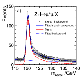
The Higgsstrahlung process provides the opportunity to study the couplings of the Higgs boson in a model-independent manner. This is unique to an electron-positron collider, where the clean experimental environment and the relatively low SM cross sections for background processes allow $\mathup{{{\mathup{{{e}}}}}^{\scriptstyle{+}}}\mathup{{{\mathup{{{e}}}}}^{\scriptstyle{-}}}\to\mathup{{{H}}}\mathup{{{Z}}}$ events to be selected based solely on the measurement of the four-momentum of the $\mathup{{{Z}}}$ boson, regardless of how the Higgs boson decays. The clearest topologies occur for $\mathup{{{Z}}}\to\mathup{{{\mathup{{{e}}}}}^{\scriptstyle{+}}}\mathup{{{\mathup{{{e}}}}}^{\scriptstyle{-}}}$ and $\mathup{{{Z}}}\to\mathup{{}^{\scriptstyle{+}}}\mathup{{}^{\scriptstyle{-}}}$ decays, which can be identified by first requiring that the measured di-lepton invariant mass $m_{\ell\ell}$ is consistent with $m_{\mathup{{{Z}}}}$. The four-momentum of the system recoiling against the $\mathup{{{Z}}}$ boson is obtained from $E_{\mathrm{rec}}=\sqrt{s}-E_{\ell\ell}$ and $\vec{p}_{\mathrm{rec}}=-\vec{p}_{\ell\ell}$. In $\mathup{{{\mathup{{{e}}}}}^{\scriptstyle{+}}}\mathup{{{\mathup{{{e}}}}}^{\scriptstyle{-}}}\to\mathup{{{H}}}\mathup{{{Z}}}$ events, the invariant mass of this recoiling system, $m_{\mathrm{rec}}$, will peak at $m_{\mathup{{{H}}}}$. Fig. 2 shows the simulated recoil mass distribution in the ILD bib:ILD_LOI detector concept for 250 $\text{fb}^{-1}$ of ILC data at $\sqrt{s}=250\,\text{GeV}$ with beam polarisation $P(\mathup{{{\mathup{{{e}}}}}^{\scriptstyle{-}}},\mathup{{{\mathup{{{e}}}}}^{\scriptstyle{+}}})=(-0.8,\,+0.3)$; by combining both $\mathup{{{Z}}}\to\mathup{{}^{\scriptstyle{+}}}\mathup{{}^{\scriptstyle{-}}}$ and $\mathup{{{Z}}}\to\mathup{{{\mathup{{{e}}}}}^{\scriptstyle{+}}}\mathup{{{\mathup{{{e}}}}}^{\scriptstyle{-}}}$ decays, $\sigma(\mathup{{{H}}}\mathup{{{Z}}})$ can be measured to 2.6 %, leading to a determination of $g_{\mathup{{{H}}}\mathup{{{Z}}}\mathup{{{Z}}}}$ with a precision of 1.3 % bib:ILC_Physics_TDR ; bib:ILD_LOI ; bib:Li .

Figure 2: The recoil mass distribution for the Higgsstrahlung process for a) $\mathup{{{Z}}}\rightarrow\mathup{{}^{\scriptstyle{+}}}\mathup{{}^{\scriptstyle{-}}}$ and b) $\mathup{{{Z}}}\rightarrow\mathup{{{\mathup{{{e}}}}}^{\scriptstyle{+}}}\mathup{{{\mathup{{{e}}}}}^{\scriptstyle{-}}}$ at $\sqrt{s}=250\,\text{GeV}$. The results are shown for $P(\mathup{{{e}}}^{-},\mathup{{{e}}}^{+})=(-80\,\%,+30\,\%)$ beam polarisation. Taken from bib:ILD_LOI .

1.3 Recoil mass measurement at different centre-of-mass energies

The narrowness of the recoil mass peak is an important factor in determining the precision to which $g_{\mathup{{{H}}}\mathup{{{Z}}}\mathup{{{Z}}}}$ can be measured. The recoil mass can be expressed as

$$m_{\text{rec}}^{2} =(\sqrt{s}-E_{\ell\ell})^{2}-\vec{p}_{\ell\ell}^{2}=s-2\sqrt{s}\,E_{\ell\ell}+E^{2}_{\ell\ell}-\vec{p}_{\ell\ell}^{2}$$

$$=s-2\sqrt{s}\,(E_{\ell 1}+E_{\ell 2})+m^{2}_{\ell\ell}\,,$$

where $\sqrt{s}$ is the centre-of-mass energy and $E_{\ell 1}$ and $E_{\ell 2}$ are the energies of the two leptons. Since $m_{\ell\ell}$ will peak narrowly around $m_{\mathup{{{Z}}}}$, it can be seen that the width of the recoil mass peak scales with both $\sqrt{s}$ and the lepton energy (or momentum) resolution. For high-momenta muons, where multiple scattering in the tracking chambers is relatively unimportant, the fractional momentum resolution $\sigma_{p}/p$ will scale approximately as the transverse momentum $p_{\mathrm{T}}$, thus $\sigma_{E_{\ell}}$ will scale quadratically as $p\cdot p_{\mathrm{T}}$. Consequently, in the range $\sqrt{s}=250-500\,\text{GeV}$, where the energy of the fermions from the $\mathup{{{Z}}}$ decay approximately scales as $\sqrt{s}$, the width of the recoil mass distribution increases significantly with increasing centre-of-mass energy. For this reason, the leptonic recoil mass analysis leads to a higher precision on $g_{\mathup{{{H}}}\mathup{{{Z}}}\mathup{{{Z}}}}$ for $\sqrt{s}\sim 250\,\text{GeV}$ bib:ILC_Physics_TDR , where the $\sigma(\mathup{{{H}}}\mathup{{{Z}}})$ is largest and the reconstructed recoil mass peak is relatively narrow. This has been one of the strongest arguments for the initial operation of the ILC at a relatively low centre-of-mass energy. This argument does not apply to the recoil mass measurement with hadronic $\mathup{{{Z}}}\to\mathup{{{q}}}\mathup{{\overline{{\mathup{{{q}}}}}}}$ decays since the recoil mass resolution depends less strongly on $\sqrt{s}$ than for leptonic final states because the jet energy resolution for the linear collider detector concepts scales linearly with energy, $\sigma_{E}\sim 0.03E$ bib:Thomson . Although the hadronic recoil mass measurement has been considered previously bib:Miyamoto , this paper presents the first detailed study of its potential.

2 Monte Carlo Samples, Detector Simulation and Event Reconstruction

The CLIC results presented in this paper are based on detailed Monte Carlo (MC) simulation using: a full set of SM background processes; a detailed Geant4 bib:Agostinelli ; bib:Allison simulation of the CLIC_ILD detector concept bib:CLIC_Physics_CDR ; and a full reconstruction of the simulated events.

2.1 Monte Carlo event generation

The simulated SM event samples were generated using the WHIZARD 1.95 bib:Whizard program. The expected energy spectra for the CLIC beams, including the effects from beamstrahlung and the intrinsic machine energy spread, were used for the initial-state electrons and positrons. The process of fragmentation and hadronisation of final-state quarks and gluons was simulated using PYTHIA 6.4 bib:PYTHIA with a parameter set bib:OPAL that was tuned to OPAL $\mathup{{{\mathup{{{e}}}}}^{\scriptstyle{+}}}\mathup{{{\mathup{{{e}}}}}^{\scriptstyle{-}}}$ data recorded at LEP. The decays of $\tau$ leptons were simulated using the TAUOLA package bib:tauola . The mass of the Higgs boson was taken to be $m_{\mathup{{{H}}}}=126\,\text{GeV}$ and the decays of the Higgs boson were simulated using PYTHIA with the branching fractions of bib:HiggsBR . A dedicated sample of $\mathup{{{\mathup{{{e}}}}}^{\scriptstyle{+}}}\mathup{{{\mathup{{{e}}}}}^{\scriptstyle{-}}}\to\mathup{{{H}}}\mathup{{{Z}}}$ events with Higgs decays to “invisible” long-lived neutral particles was produced by artificially setting the Higgs boson lifetime to infinity. Because of the 0.5 ns bunch spacing in the CLIC beams, the pile-up of beam-induced backgrounds from the $\mathup{}\mathup{}\to\text{hadrons}$ process was included in the simulated event samples to ensure its effect on the event reconstruction was accounted for.

2.2 CLIC detector simulation and event reconstruction

The Geant4-based Mokka bib:Mokka program was used to simulate the detector response of the CLIC_ILD detector concept bib:CLIC_Physics_CDR . The QGSP_BERT physics list was used to model the hadronic interactions of particles in the detectors. The hit digitisation and the event reconstruction were performed using the Marlin bib:Marlin software packages. Particle flow reconstruction was performed using PandoraPFA bib:Thomson ; bib:Marshall . An algorithm, using the individual reconstructed particles, was used to identify and remove approximately 90 % of the out-of-time background due to pile-up from $\mathup{}\mathup{}\to\text{hadrons}$; here the Loose particle flow object selection, described in bib:CLIC_Physics_CDR , was used.

Jet finding was performed using the FastJet bib:Fastjet package. Because of the presence of pile-up from $\mathup{}\mathup{}\to\text{hadrons}$, the ee_kt (Durham) algorithm employed at LEP is not effective as it clusters particles from pile-up into the reconstructed jets. Instead, the hadron-collider inspired $k_{t}$ algorithm, with the distance parameter $R$ based on $\Delta\eta$ and $\Delta\phi$, was used with $R=\pi/2$. This algorithm allows particles to be clustered into “beam jets”, aligned with the beam axis, in addition to jets seeded by high-momentum particles. Background from the pile-up of $\mathup{}\mathup{}\to\text{hadrons}$ can, to a large degree, be removed by ignoring particles in the “beam jets”, largely mitigating the impact of the beam background.

The hadronic recoil mass study, presented in this paper, covers a wide range of $\mathup{{{H}}}\mathup{{{Z}}}(\mathup{{{Z}}}\to\mathup{{{q}}}\mathup{{\overline{{\mathup{{{q}}}}}}})$ final-state topologies ranging from two jets where Higgs decays to long-lived neutral particles, $\mathup{{{\mathup{{{e}}}}}^{\scriptstyle{+}}}\mathup{{{\mathup{{{e}}}}}^{\scriptstyle{-}}}\to\mathup{{{H}}}\mathup{{{Z}}}\to(\text{invis.})(\mathup{{{q}}}\mathup{{\overline{{\mathup{{{q}}}}}}})$, to six-jet toplogies from, for example, $\mathup{{{\mathup{{{e}}}}}^{\scriptstyle{+}}}\mathup{{{\mathup{{{e}}}}}^{\scriptstyle{-}}}\to\mathup{{{H}}}\mathup{{{Z}}}\to(\mathup{{{W}}}\mathup{{{W}}}^{*}\to\mathup{{{q}}}\mathup{{\overline{{\mathup{{{q}}}}}}}\mathup{{{q}}}\mathup{{\overline{{\mathup{{{q}}}}}}})(\mathup{{{q}}}\mathup{{\overline{{\mathup{{{q}}}}}}})$. For this reason, each reconstructed event is clustered into two-, three-, four-, five- and six-jet topologies, with “$y$-cut” variables used to indicate the underlying physical topology. For example, if an event is forced into a three-jet topology, $y_{34}$ is the $k_{t}$ value at which the event would be reconstructed as four jets and $y_{23}$ is the $k_{t}$ value at which the event would be reconstructed as two jets.

2.3 ILC detector simulation and event reconstruction

The event generation and reconstruction for the ILC studies, presented in section 4, follows closely that described above. The main differences are: i) the ILC beam spectrum, where the effects of beamstrahlung are less pronounced, was used, ii) the detector simulation used the ILD detector concept for the ILC, rather than the CLIC_ILD model adapted for CLIC; and iii) the much longer bunch spacing at the ILC means that only in-time background from $\mathup{}\mathup{}\to\text{hadrons}$ needs to be included.

3 Hadronic Recoil Mass Measurement at CLIC

In the process $\mathup{{{\mathup{{{e}}}}}^{\scriptstyle{+}}}\mathup{{{\mathup{{{e}}}}}^{\scriptstyle{-}}}\to\mathup{{{H}}}\mathup{{{Z}}}$ it is possible to cleanly identify $\mathup{{{Z}}}\to\mathup{{{\mathup{{{e}}}}}^{\scriptstyle{+}}}\mathup{{{\mathup{{{e}}}}}^{\scriptstyle{-}}}$ and $\mathup{{{Z}}}\to\mathup{{}^{\scriptstyle{+}}}\mathup{{}^{\scriptstyle{-}}}$ decays regardless of the $\mathup{{{H}}}$ decay mode. Consequently, the selection efficiency is almost independent of the nature of the $\mathup{{{H}}}$ decay. For $\mathup{{{Z}}}\to\mathup{{{q}}}\mathup{{\overline{{\mathup{{{q}}}}}}}$ decays, the selection efficiency will depend more strongly on the Higgs decay mode. For example, in $(\mathup{{{H}}}\to\mathup{{{b}}}\mathup{{\overline{{\mathup{{{b}}}}}}})(\mathup{{{Z}}}\to\mathup{{{q}}}\mathup{{\overline{{\mathup{{{q}}}}}}})$ events, the reconstruction of the $\mathup{{{Z}}}$ boson is complicated by mis-associations of particles to jets and by the three-fold ambiguity in associating four jets to the $\mathup{{{Z}}}$ and $\mathup{{{H}}}$. These ambiguities will increase with the number of jets in the final state. For this reason, it is much more difficult to construct an event selection, based only on the reconstructed candidate $\mathup{{{Z}}}\to\mathup{{{q}}}\mathup{{\overline{{\mathup{{{q}}}}}}}$ decay, with a selection efficiency that is independent of the Higgs decay mode. Nevertheless it is possible to minimise this dependence. The strategy adopted here is to: i) separate all simulated events into candidates for Higgs decays to “invisible” long-lived neutral particles and decays to visible final states; ii) identify the di-jet system that is the best candidate for the $\mathup{{{Z}}}\to\mathup{{{q}}}\mathup{{\overline{{\mathup{{{q}}}}}}}$ decay; iii) reject events consistent with a number of clear background topologies using the information from the whole event; iv) identify $\mathup{{{H}}}\mathup{{{Z}}}(\mathup{{{Z}}}\to\mathup{{{q}}}\mathup{{\overline{{\mathup{{{q}}}}}}})$ events solely based on the properties from the candidate $\mathup{{{Z}}}\to\mathup{{{q}}}\mathup{{\overline{{\mathup{{{q}}}}}}}$ decay, first for the candidate visible Higgs decays and then for the candidate invisible Higgs decays; and v) combine the results into a single measurement of $\sigma(\mathup{{{H}}}\mathup{{{Z}}})$.

3.1 Separation into candidate visible and invisible Higgs decay samples

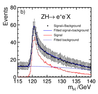
Hadronic events are selected by forcing each event into a two-jet topology and requiring at least three charged particles in each jet. The surviving events are then divided into candidates for either visible $\mathup{{{H}}}$ decays or invisible $\mathup{{{H}}}$ decays, in both cases produced in association with a $\mathup{{{Z}}}\to\mathup{{{q}}}\mathup{{\overline{{\mathup{{{q}}}}}}}$. Events are categorised as potential invisible $\mathup{{{H}}}$ decays on the basis of the $y$-cut values in the $k_{t}$ jet-finding algorithm. For invisible $\mathup{{{H}}}$ decays, only the $\mathup{{{Z}}}\to\mathup{{{q}}}\mathup{{\overline{{\mathup{{{q}}}}}}}$ system is visible in the detector, typically resulting in a two-jet topology (with the possibility that QCD radiation can increase the number of reconstructed jets). Consequently, invisible $\mathup{{{H}}}$ decays will have small values of $y_{23}$ and $y_{34}$, the variables respectively representing the $k_{t}$ value at which an event transitions from two to three jets and from three to four jets, as indicated in Fig. 3. Events are categorised as candidate invisible $\mathup{{{H}}}$ decays if $-\log_{10}(y_{23})>2.0$ and $-\log_{10}(y_{34})>3.0$. Due to gluon radiation in the parton shower, only 74 % of the simulated $\mathup{{{H}}}\mathup{{{Z}}}\,(\mathup{{{Z}}}\rightarrow\mathup{{{q}}}\mathup{{\overline{{\mathup{{{q}}}}}}})$ events with invisible $\mathup{{{H}}}$ decays are placed in this two-jet topology candidate invisible $\mathup{{{H}}}$ decay sample. To improve the efficiency for correctly categorising SM Higgs decays with low-energy leptons, for example $\mathup{{{H}}}\to\mathup{{{W}}}\mathup{{{W}}}^{*}\to\mathup{}\mathup{}\mathup{}\mathup{}$, events with $-\log_{10}(y_{23})<2.5$ and $-\log_{10}(y_{34})<3.5$ are forced into three jets and are excluded from the invisible Higgs decay sample if the lowest-energy jet has fewer than four reconstructed tracks or contains an identified $\mathup{{{e}}}^{\pm}/\mathup{}^{\pm}$ with energy $E>5\,\text{GeV}$. Only 2.2 % of simulated $\mathup{{{H}}}\mathup{{{Z}}}$ events with SM Higgs decays end up in the candidate invisible Higgs sample.

Figure 3: The distributions of $-\log_{10}(y_{23})$ and $-\log_{10}(y_{34})$ for simulated $\mathup{{{H}}}\mathup{{{Z}}}\,(\mathup{{{Z}}}\to\mathup{{{q}}}\mathup{{\overline{{\mathup{{{q}}}}}}})$ events for visible and invisible Higgs decays at $\sqrt{s}=350\,\text{GeV}$. The distributions are normalised to an integrated luminosity of 500 $\text{fb}^{-1}$. The distribution for the invisible $\mathup{{{H}}}$ decays assumes a 100 % branching fraction into invisible decay modes. The vertical lines with arrows indicate the cut values used in this analysis.

3.2 Recoil mass reconstruction

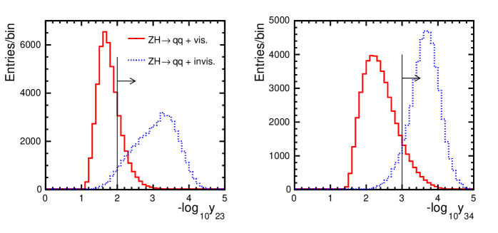
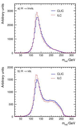
For each candidate $\mathup{{{H}}}\mathup{{{Z}}}(\mathup{{{Z}}}\to\mathup{{{q}}}\mathup{{\overline{{\mathup{{{q}}}}}}})$ event, the recoil mass is calculated from $m_{\mathrm{rec}}^{2}=(\sqrt{s}-E_{\mathup{{{q}}}\mathup{{\overline{{\mathup{{{q}}}}}}}})^{2}-\vec{p}_{\mathup{{{q}}}\mathup{{\overline{{\mathup{{{q}}}}}}}}^{2}$, where $E_{\mathup{{{q}}}\mathup{{\overline{{\mathup{{{q}}}}}}}}$ and $\vec{p}_{\mathup{{{q}}}\mathup{{\overline{{\mathup{{{q}}}}}}}}$ are the summed energy and momentum of the di-jet system from the identified candidate $\mathup{{{Z}}}\to\mathup{{{q}}}\mathup{{\overline{{\mathup{{{q}}}}}}}$ decay. In the case of the candidate invisible Higgs decay sample, the two jets are assumed to be from $\mathup{{{Z}}}\to\mathup{{{q}}}\mathup{{\overline{{\mathup{{{q}}}}}}}$. The resulting recoil mass distribution for candidate invisible Higgs decays, which is strongly peaked around $m_{\mathrm{rec}}\sim m_{\mathup{{{H}}}}$, is shown in Fig. 4a. In the case of the candidate visible Higgs decay sample, the situation is more complicated as this sample encompasses many different $\mathup{{{H}}}\mathup{{{Z}}}$ event topologies. For example, $\mathup{{{H}}}\to\mathup{{{b}}}\mathup{{\overline{{\mathup{{{b}}}}}}}$ decays will result in a four-quark $\mathup{{{H}}}\mathup{{{Z}}}$ final state, usually yielding four jets, whereas, $\mathup{{{H}}}\to\mathup{{{W}}}\mathup{{{W}}}^{*}\to\mathup{{{q}}}\mathup{{\overline{{\mathup{{{q}}}}}}}\ell\mathup{}$ and $\mathup{{{H}}}\to\mathup{{{W}}}\mathup{{{W}}}^{*}\to\mathup{{{q}}}\mathup{{\overline{{\mathup{{{q}}}}}}}\mathup{{{q}}}\mathup{{\overline{{\mathup{{{q}}}}}}}$ decays will respectively usually yield five- and six-jet final states. In all cases gluon radiation in the parton shower can increase the reconstructed jet multiplicity relative to the tree-level expectation.

In order to achieve the desired (near) model independence of the analysis, it is necessary to have a similar quality of recoil mass reconstruction for all Higgs boson visible decay modes. This hinges on the correct identification and reconstruction of the $\mathup{{{Z}}}\to\mathup{{{q}}}\mathup{{\overline{{\mathup{{{q}}}}}}}$ di-jet system. The first stage is to force events in the candidate visible Higgs decay sample into a four-jet topology. From the three possible di-jet combinations, the di-jet system with invariant mass $m_{\mathup{{{q}}}\mathup{{\overline{{\mathup{{{q}}}}}}}}$ closest to $m_{\mathup{{{Z}}}}$ is identified as the candidate $\mathup{{{Z}}}\to\mathup{{{q}}}\mathup{{\overline{{\mathup{{{q}}}}}}}$ decay and its energy and momentum are used to calculate the recoil mass $m_{\mathrm{rec}}$. In selecting the candidate $\mathup{{{Z}}}$ decay, only jets containing more than three charged particles are considered. To improve the reconstruction of higher-jet-multiplicity final states, such as $\mathup{{{H}}}\to\mathup{{{W}}}\mathup{{{W}}}^{*}\to\mathup{{{q}}}\mathup{{\overline{{\mathup{{{q}}}}}}}\mathup{{{q}}}\mathup{{\overline{{\mathup{{{q}}}}}}}$, each event is also forced into five jets and the di-jet system with mass closest to $m_{\mathup{{{Z}}}}$ is again identified as the candidate $\mathup{{{Z}}}\to\mathup{{{q}}}\mathup{{\overline{{\mathup{{{q}}}}}}}$ decay. The five-jet topology is only used if $-\log_{10}(y_{45})>3.5$ and both $m_{\mathup{{{q}}}\mathup{{\overline{{\mathup{{{q}}}}}}}}$ and $m_{\mathrm{rec}}$ are respectively closer to $m_{\mathup{{{Z}}}}$ and $m_{\mathup{{{H}}}}$ than the corresponding values from the four-jet reconstruction. Even in the genuine six-parton topology $\mathup{{{H}}}\mathup{{{Z}}}\to(\mathup{{{W}}}\mathup{{{W}}}^{*})\mathup{{{q}}}\mathup{{\overline{{\mathup{{{q}}}}}}}\to(\mathup{{{q}}}\mathup{{\overline{{\mathup{{{q}}}}}}}\mathup{{{q}}}\mathup{{\overline{{\mathup{{{q}}}}}}})\mathup{{{q}}}\mathup{{\overline{{\mathup{{{q}}}}}}}$ only 13 % of events are reconstructed as five jets, for the remainder, the four-jet reconstruction is preferred. However, provided the jets from the $\mathup{{{Z}}}\to\mathup{{{q}}}\mathup{{\overline{{\mathup{{{q}}}}}}}$ decay are correctly identified, there is no need to correctly reconstruct the recoiling system as only the properties of the $\mathup{{{Z}}}\to\mathup{{{q}}}\mathup{{\overline{{\mathup{{{q}}}}}}}$ decay are used in the subsequent analysis. For this reason, allowing the possibility of reconstructing events as six jets was found not to improve the overall recoil mass reconstruction. Fig. 4b shows the resulting recoil mass distribution for simulated $\mathup{{{H}}}\mathup{{{Z}}}$ events with $\mathup{{{H}}}\to\mathup{{{b}}}\mathup{{\overline{{\mathup{{{b}}}}}}}$, $\mathup{{{H}}}\to\mathup{{{W}}}\mathup{{{W}}}^{*}\to\mathup{{{q}}}\mathup{{\overline{{\mathup{{{q}}}}}}}\mathup{{{q}}}\mathup{{\overline{{\mathup{{{q}}}}}}}$ and $\mathup{{{H}}}\to\mathup{{}^{\scriptstyle{+}}}\mathup{{}^{\scriptstyle{-}}}$. Despite the very different final states, similar recoil mass distributions are obtained.

Figure 4: a) The reconstructed hadronic recoil mass distribution for the candidate $\mathup{{{H}}}\mathup{{{Z}}}$ events with $\mathup{{{Z}}}\to\mathup{{{q}}}\mathup{{\overline{{\mathup{{{q}}}}}}}$ and $\mathup{{{H}}}\to\text{invis.}$ b) The reconstructed hadronic recoil mass distributions for candidate $\mathup{{{H}}}\mathup{{{Z}}}(\mathup{{{Z}}}\to\mathup{{{q}}}\mathup{{\overline{{\mathup{{{q}}}}}}})$ and either $\mathup{{{H}}}\to\mathup{{{b}}}\mathup{{\overline{{\mathup{{{b}}}}}}}$, $\mathup{{{H}}}\to\mathup{{{W}}}\mathup{{{W}}}^{*}\to\mathup{{{q}}}\mathup{{\overline{{\mathup{{{q}}}}}}}\mathup{{{q}}}\mathup{{\overline{{\mathup{{{q}}}}}}}$ or $\mathup{{{H}}}\to\mathup{{}^{\scriptstyle{+}}}\mathup{{}^{\scriptstyle{-}}}$. In each case the distributions are normalised to unit area. An underflow (not shown) contains the small fraction of events where no good $\mathup{{{Z}}}\to\mathup{{{q}}}\mathup{{\overline{{\mathup{{{q}}}}}}}$ candidate is identified.

3.3 Preselection

After dividing all events into either candidates for visible or invisible Higgs decays and having identified the two jets forming the candidate $\mathup{{{Z}}}\to\mathup{{{q}}}\mathup{{\overline{{\mathup{{{q}}}}}}}$ system, preselection cuts are applied to reduce backgrounds from larger cross section SM processes such as $\mathup{{{\mathup{{{e}}}}}^{\scriptstyle{+}}}\mathup{{{\mathup{{{e}}}}}^{\scriptstyle{-}}}\to\mathup{{{q}}}\mathup{{\overline{{\mathup{{{q}}}}}}}$ and $\mathup{{{\mathup{{{e}}}}}^{\scriptstyle{+}}}\mathup{{{\mathup{{{e}}}}}^{\scriptstyle{-}}}\to\mathup{{{q}}}\mathup{{\overline{{\mathup{{{q}}}}}}}\mathup{{{q}}}\mathup{{\overline{{\mathup{{{q}}}}}}}$. Cuts are based on the invariant mass of the $\mathup{{{Z}}}\to\mathup{{{q}}}\mathup{{\overline{{\mathup{{{q}}}}}}}$ candidate, $m_{\mathup{{{q}}}\mathup{{\overline{{\mathup{{{q}}}}}}}}$, and corresponding recoil mass, $m_{\mathrm{rec}}$. In addition, the invariant mass of all the visible particles not originating from the candidate $\mathup{{{Z}}}\to\mathup{{{q}}}\mathup{{\overline{{\mathup{{{q}}}}}}}$ decay, $m^{\prime}_{\mathup{{{q}}}\mathup{{\overline{{\mathup{{{q}}}}}}}}$, is calculated. It is important to note that $m^{\prime}_{\mathup{{{q}}}\mathup{{\overline{{\mathup{{{q}}}}}}}}$ is only used to reject specific background topologies in the preselection and is not used in the main selection; in $\mathup{{{H}}}\mathup{{{Z}}}$ events $m^{\prime}_{\mathup{{{q}}}\mathup{{\overline{{\mathup{{{q}}}}}}}}$ will depend strongly on the Higgs decay mode. The preselection cuts (most of which are common to the visible and invisible Higgs selections) are:

• the event must be broadly consistent with being $\mathup{{{H}}}\mathup{{{Z}}}$, $70\,\text{GeV}<m_{\mathup{{{q}}}\mathup{{\overline{{\mathup{{{q}}}}}}}}<110\,\text{GeV}$ and $80\,\text{GeV}<m_{\mathrm{rec}}<200\,\text{GeV}$.

• background from $\mathup{{{\mathup{{{e}}}}}^{\scriptstyle{+}}}\mathup{{{\mathup{{{e}}}}}^{\scriptstyle{-}}}\to\mathup{{{q}}}\mathup{{\overline{{\mathup{{{q}}}}}}}$ is suppressed by removing events with net transverse momentum $p_{\mathrm{T}}<20\,\text{GeV}$ and $-\log_{10}(y_{34})>2.5$, indicating a final-state system consisting of fewer than four primary particles.

• events in the invisible Higgs decay sample are rejected if $|\cos\theta_{\text{mis}}|>0.7$, where $\theta_{\text{mis}}$ is the polar angle of the missing momentum vector, almost completely eliminating the contribution from $\mathup{{{\mathup{{{e}}}}}^{\scriptstyle{+}}}\mathup{{{\mathup{{{e}}}}}^{\scriptstyle{-}}}\to\mathup{{{q}}}\mathup{{\overline{{\mathup{{{q}}}}}}}$ with unobserved initial-state radiation (ISR).

• events in the invisible Higgs decay sample are rejected if there is an isolated identified $\mathup{{{e}}}^{\pm}/\mathup{}^{\pm}$ with energy $E_{\ell}>10\,$GeV, suppressing background from $\mathup{{{W}}}\mathup{{{W}}}\to\mathup{{{q}}}\mathup{{\overline{{\mathup{{{q}}}}}}}\ell\mathup{}$.

• background from $\mathup{{{\mathup{{{e}}}}}^{\scriptstyle{+}}}\mathup{{{\mathup{{{e}}}}}^{\scriptstyle{-}}}\to\mathup{{{q}}}\mathup{{\overline{{\mathup{{{q}}}}}}}$ with unobserved ISR, including radiative return to the $\mathup{{{Z}}}$ resonance, is suppressed by rejecting events with net transverse momentum $p_{\mathrm{T}}<20\,\text{GeV}$ and $|\cos\theta_{\text{mis}}|>0.9$.

• the background from $\mathup{{{\mathup{{{e}}}}}^{\scriptstyle{+}}}\mathup{{{\mathup{{{e}}}}}^{\scriptstyle{-}}}\to\mathup{{{W}}}\mathup{{{W}}}\rightarrow\mathup{{{q}}}\mathup{{\overline{{\mathup{{{q}}}}}}}\mathup{{{q}}}\mathup{{\overline{{\mathup{{{q}}}}}}}$ is suppressed by forcing events into four jets and selecting the di-jet pair with the mass $m_{\mathup{{{q}}}\mathup{{\overline{{\mathup{{{q}}}}}}}}$ closest to $m_{\mathup{{{W}}}}$. Events are rejected if $p_{\mathrm{T}}<20\,\text{GeV}$ and $65\,\text{GeV}<m_{\mathup{{{q}}}\mathup{{\overline{{\mathup{{{q}}}}}}}}<100\,\text{GeV}$ and $65\,\text{GeV}<m^{\prime}_{\mathup{{{q}}}\mathup{{\overline{{\mathup{{{q}}}}}}}}<100\,\text{GeV}$, where $m^{\prime}_{\mathup{{{q}}}\mathup{{\overline{{\mathup{{{q}}}}}}}}$ is the measured invariant mass of the second di-jet pair.

• the background from $\mathup{{{\mathup{{{e}}}}}^{\scriptstyle{+}}}\mathup{{{\mathup{{{e}}}}}^{\scriptstyle{-}}}\to\mathup{{{Z}}}\mathup{{{Z}}}\rightarrow\mathup{{{q}}}\mathup{{\overline{{\mathup{{{q}}}}}}}\mathup{{{q}}}\mathup{{\overline{{\mathup{{{q}}}}}}}$ is suppressed in a similar manner. Events are forced into four jets and the di-jet pair with the $m_{\mathup{{{q}}}\mathup{{\overline{{\mathup{{{q}}}}}}}}$ closest to $m_{\mathup{{{Z}}}}$ is identified. Events are rejected if $p_{\mathrm{T}}<20\,\text{GeV}$ and $70\,\text{GeV}<m_{\mathup{{{q}}}\mathup{{\overline{{\mathup{{{q}}}}}}}}<105\,\text{GeV}$ and $70\,\text{GeV}<m^{\prime}_{\mathup{{{q}}}\mathup{{\overline{{\mathup{{{q}}}}}}}}<105\,\text{GeV}$, where $m^{\prime}_{\mathup{{{q}}}\mathup{{\overline{{\mathup{{{q}}}}}}}}$ is the measured mass of the second di-jet pair.

The effects of the preselection cuts are summarised in Tab. 2. The events passing the preselection cuts are put forward as candidate $\mathup{{{H}}}\mathup{{{Z}}}(\mathup{{{Z}}}\to\mathup{{{q}}}\mathup{{\overline{{\mathup{{{q}}}}}}})$ events with either: i) visible $\mathup{{{H}}}$ decay products; or ii) invisible $\mathup{{{H}}}$ decay products, depending on whether the event was consistent with a two-jet topology or not. The first two cuts listed above result in the largest loss of signal efficiency for the visible Higgs decay selection. The $\mathup{{{q}}}\mathup{{\overline{{\mathup{{{q}}}}}}}\ell\mathup{}$ background in the visible Higgs decay preselection could have been significantly reduced by rejecting events with visible high-energy isolated leptons, but this would have introduced a bias against $\mathup{{{H}}}$ decays with leptons in the final state.

Final state	$\sigma/\text{fb}$	$\varepsilon^{\text{vis.}}_{\text{presel}}$	$\varepsilon^{\text{invis.}}_{\text{presel}}$	$N^{\text{vis.}}_{\text{presel}}$	$N^{\text{invis.}}_{\text{presel}}$
$\mathup{{{q}}}\mathup{{\overline{{\mathup{{{q}}}}}}}$	25180	0.4 %	$-$ %	54570	0
$\mathup{{{q}}}\mathup{{\overline{{\mathup{{{q}}}}}}}\ell\mathup{}$	5914	11.2 %	0.9 %	326420	26060
$\mathup{{{q}}}\mathup{{\overline{{\mathup{{{q}}}}}}}\mathup{{{q}}}\mathup{{\overline{{\mathup{{{q}}}}}}}$	5847	3.8 %	$-$ %	110520	0
$\mathup{{{q}}}\mathup{{\overline{{\mathup{{{q}}}}}}}\ell\ell$	1704	1.5 %	$-$ %	13260	60
$\mathup{{{q}}}\mathup{{\overline{{\mathup{{{q}}}}}}}\mathup{}\mathup{{\overline{{\upnu}}}}$	325	0.6 %	14.8 %	1050	24180
$\mathup{{{H}}}\mathup{{{\mathup{}}}{}_{\scriptstyle{\!\mathup{{{e}}}}}}\mathup{{\overline{{\mathup{}}}}{}_{\scriptstyle{\!\mathup{{{e}}}}}}$	52	2.5 %	5.6 %	640	1430
$\mathup{{{H}}}\mathup{{{Z}}}$; $\mathup{{{Z}}}\to\mathup{{{q}}}\mathup{{\overline{{\mathup{{{q}}}}}}}$	93	42.0 %	0.2 %	19630	80
$\mathup{{{H}}}\to\text{invis.}$  (100 %) ​​​​​​​​​​​​​	93	0.6 %	48.6 %	300	22710

Table 2: Summary of the effects of the preselection cuts for the the visible and invisible recoil mass analyses. The efficiencies $\varepsilon$ include the effects of the preselection cuts and the division into the candidate visible and invisible Higgs decay samples. The expected numbers of events passing the preselection cuts correspond to an integrated luminosity of $500\,\text{fb}^{-1}$ at CLIC, assuming unpolarised beams at $\sqrt{s}=350\,\text{GeV}$. The numbers shown for the invisible Higgs decay modes correspond to a 100 % branching ratio.

3.4 Selection of HZ$\to$q$\overline{\text{q}}$ with visible Higgs decays

After preselection, the main backgrounds in the visible Higgs decay analysis arise from $\mathup{{{\mathup{{{e}}}}}^{\scriptstyle{+}}}\mathup{{{\mathup{{{e}}}}}^{\scriptstyle{-}}}\to\mathup{{{q}}}\mathup{{\overline{{\mathup{{{q}}}}}}}\ell\mathup{}$ and $\mathup{{{\mathup{{{e}}}}}^{\scriptstyle{+}}}\mathup{{{\mathup{{{e}}}}}^{\scriptstyle{-}}}\to\mathup{{{q}}}\mathup{{\overline{{\mathup{{{q}}}}}}}\mathup{{{q}}}\mathup{{\overline{{\mathup{{{q}}}}}}}$, dominated by $\mathup{{{W}}}\mathup{{{W}}}$, single-$\mathup{{{W}}}$ ($\mathup{{{W}}}\mathup{{{e}}}\mathup{{{\mathup{}}}{}_{\scriptstyle{\!\mathup{{{e}}}}}}$) and $\mathup{{{Z}}}\mathup{{{Z}}}$ processes. The event selection is based entirely on the reconstructed candidate $\mathup{{{Z}}}\to\mathup{{{q}}}\mathup{{\overline{{\mathup{{{q}}}}}}}$ decay in the event. The properties of the remainder of the event (or the event as a whole) are not used as their inclusion would break the desired model independence of the selection. For example, the background from $\mathup{{{\mathup{{{e}}}}}^{\scriptstyle{+}}}\mathup{{{\mathup{{{e}}}}}^{\scriptstyle{-}}}\to\mathup{{{q}}}\mathup{{\overline{{\mathup{{{q}}}}}}}\ell\mathup{}$ can be significantly reduced by placing a lower bound on the total visible energy in the event, however such a cut would bias the selection against Higgs decays with missing energy, such as ${\mathup{{{H}}}\to\mathup{{}^{\scriptstyle{+}}}\mathup{{}^{\scriptstyle{-}}}}$.

The event selection uses a relative likelihood approach with discriminant variables based on the properties of candidate $\mathup{{{Z}}}\to\mathup{{{q}}}\mathup{{\overline{{\mathup{{{q}}}}}}}$ decay. Two event categories are considered: a) the $\mathup{{{\mathup{{{e}}}}}^{\scriptstyle{+}}}\mathup{{{\mathup{{{e}}}}}^{\scriptstyle{-}}}\to\mathup{{{H}}}\mathup{{{Z}}}\to\mathup{{{H}}}\mathup{{{q}}}\mathup{{\overline{{\mathup{{{q}}}}}}}$ signal; and b) all non-Higgs background processes. The relative likelihood for an event being classified as signal is defined as

$${\cal{L}}=\frac{L_{\text{signal}}}{L_{\text{signal}}+L_{\text{back}}}\,,$$

where the individual absolute likelihood $L_{j}$ for the event class $j$ (signal or background) is formed from normalised probability distributions $P^{j}_{i}(x_{i})$ of the discriminant variables $x_{i}$ for that event class $j$:

$$L_{j}=\sigma^{j}_{\text{presel}}\times\prod_{i}^{N}P^{j}_{i}(x_{i})\,,$$

where $\sigma^{j}_{\text{presel}}$ is the cross section after preselection for event class $j$.

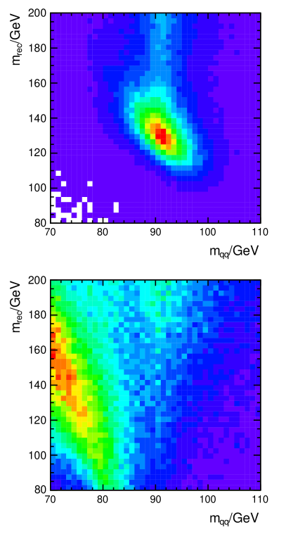
The discriminant variables used in the likelihood selection, all of which are based on the candidate $\mathup{{{Z}}}\to\mathup{{{q}}}\mathup{{\overline{{\mathup{{{q}}}}}}}$ decay, are: i) the two-dimensional distribution of $m_{\mathup{{{q}}}\mathup{{\overline{{\mathup{{{q}}}}}}}}$ and $m_{\mathrm{rec}}$; ii) the polar angle of the $\mathup{{{Z}}}$ candidate, $|\cos\theta_{\mathup{{{Z}}}}|$; and iii) the modulus of the angle of the jets from the $\mathup{{{Z}}}\to\mathup{{{q}}}\mathup{{\overline{{\mathup{{{q}}}}}}}$ decay in $\mathup{{{Z}}}$ rest frame, relative to its laboratory frame direction of motion, $|\cos\theta_{\mathup{{{q}}}}|$. The two-dimensional distributions of $m_{\mathup{{{q}}}\mathup{{\overline{{\mathup{{{q}}}}}}}}$ and $m_{\mathrm{rec}}$, are shown separately for the signal and background in Fig. 5. As expected, the $\mathup{{{H}}}\mathup{{{Z}}}$ signal events peak around $m_{\mathup{{{q}}}\mathup{{\overline{{\mathup{{{q}}}}}}}}\approx m_{\mathup{{{Z}}}}$ and $m_{\mathrm{rec}}\approx m_{\mathup{{{H}}}}$. The anti-correlation between $m_{\mathrm{rec}}$ and $m_{\mathup{{{q}}}\mathup{{\overline{{\mathup{{{q}}}}}}}}$ is expected; when the reconstructed jet energies are higher than the true energies, the reconstructed value of $m_{\mathup{{{q}}}\mathup{{\overline{{\mathup{{{q}}}}}}}}$ will be higher than $m_{\mathup{{{Z}}}}$ and $m_{\mathrm{rec}}$ will be lower than $m_{\mathup{{{H}}}}$ due to the $-2\!\sqrt{s}\,E_{\mathup{{{Z}}}}$ term in the expression for the recoil mass, $m_{\mathrm{rec}}^{2}=s-2\!\sqrt{s}\,E_{\mathup{{{Z}}}}+m_{\mathup{{{q}}}\mathup{{\overline{{\mathup{{{q}}}}}}}}^{2}\,$. The broad peaked structure in the background distribution at lower values of $m_{\mathup{{{q}}}\mathup{{\overline{{\mathup{{{q}}}}}}}}$ arises from $\mathup{{{q}}}\mathup{{\overline{{\mathup{{{q}}}}}}}\ell\mathup{}$ events (which have been forced into a four- or five-jet topology). The use of the two-dimensional distribution of $m_{\mathup{{{q}}}\mathup{{\overline{{\mathup{{{q}}}}}}}}$ versus $m_{\mathrm{rec}}$ in the likelihood accounts for the associated correlations.

Figure 5: The distribution of the reconstructed $\mathup{{{Z}}}\to\mathup{{{q}}}\mathup{{\overline{{\mathup{{{q}}}}}}}$ mass, $m_{\mathup{{{q}}}\mathup{{\overline{{\mathup{{{q}}}}}}}}$, versus the hadronic recoil mass, $m_{\mathrm{rec}}$, for $\mathup{{{H}}}\mathup{{{Z}}}(\mathup{{{Z}}}\to\mathup{{{q}}}\mathup{{\overline{{\mathup{{{q}}}}}}})$ events (top) and for all background processes (bottom). In both cases the plots show all events passing the visible Higgs preselection for CLIC operating at $\sqrt{s}=350\,\text{GeV}$.

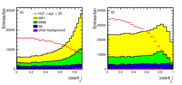
The two angular variables used in the likelihood selection are shown in Fig. 6. The discriminating power arises from the fact that the Higgs boson is a scalar particle, and the angular distributions in $\mathup{{{H}}}\mathup{{{Z}}}$ production are different from those in the dominant backgrounds which mostly arise from the production of two vector particles.

Figure 6: a) The polar angle of the reconstructed $\mathup{{{Z}}}$ candidates, $|\cos\theta_{\mathup{{{Z}}}}|$, for both signal and background events for CLIC operating at $\sqrt{s}=350\,\text{GeV}$, and b) the modulus of the angle of the jets from the $\mathup{{{Z}}}\to\mathup{{{q}}}\mathup{{\overline{{\mathup{{{q}}}}}}}$ decay relative to the $\mathup{{{Z}}}$ direction after boosting into its rest frame, $|\cos\theta_{\mathup{{{q}}}}|$. The signal and background distributions are normalised to 500 $\text{fb}^{-1}$, but the $\mathup{{{H}}}\mathup{{{Z}}}(\mathup{{{Z}}}\to\mathup{{{q}}}\mathup{{\overline{{\mathup{{{q}}}}}}})$ signal has been scaled by a factor of 25 to improve its visibility.

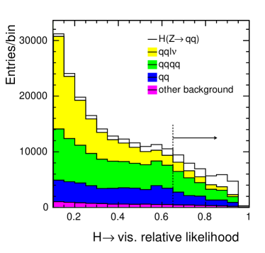
The resulting relative likelihood distribution is shown in Fig. 7. Despite the fact that the signal-to-background ratio in the preselected event sample is approximately 1:25, the likelihood selection provides good separation. The statistical precision on the cross section for $\mathup{{{H}}}\mathup{{{Z}}}$ production (where the $\mathup{{{Z}}}$ decays hadronically and the $\mathup{{{H}}}$ has SM branching fractions) is maximised with a likelihood cut of ${\cal{L}}>0.65$. The resulting efficiencies and the expected numbers of selected events for an integrated luminosity of 500 $\text{fb}^{-1}$ are shown in Tab. 3. The corresponding statistical uncertainty on the production cross section is $\pm 1.9\,\%$. The precision can be improved by extracting the number of signal events by performing a maximum-likelihood fit to the shape of the simulated likelihood distribution by varying the normalisations of the signal and background components, yielding a statistical error of

$$\Delta\sigma_{\text{vis.}} =\pm 1.7\,\%\,.$$

Figure 7: The resulting likelihood distribution for the hadronic recoil mass analysis. The distributions correspond to 500 $\text{fb}^{-1}$ of CLIC operation at $\sqrt{s}=350\,\text{GeV}$ with unpolarised electron and positron beams. The optimal likelihood cut at ${\cal{L}}=0.65$ is indicated by the arrow.

Process	$\sigma/\text{fb}$	$\varepsilon_{\text{presel}}$	$\varepsilon^{\text{vis.}}_{{\cal{L}}>0.65}$	$N_{{\cal{L}}>0.65}$
$\mathup{{{q}}}\mathup{{\overline{{\mathup{{{q}}}}}}}$	25180	0.4 %	0.07 %	8525
$\mathup{{{q}}}\mathup{{\overline{{\mathup{{{q}}}}}}}\ell\mathup{}$	5914	11.2 %	0.20 %	5767
$\mathup{{{q}}}\mathup{{\overline{{\mathup{{{q}}}}}}}\mathup{{{q}}}\mathup{{\overline{{\mathup{{{q}}}}}}}$	5847	3.8 %	0.49 %	14142
$\mathup{{{q}}}\mathup{{\overline{{\mathup{{{q}}}}}}}\ell\ell$	1704	1.5 %	0.22 %	1961
$\mathup{{{q}}}\mathup{{\overline{{\mathup{{{q}}}}}}}\mathup{}\mathup{{\overline{{\upnu}}}}$	325	0.6 %	0.04 %	60
$\mathup{{{H}}}\mathup{{{\mathup{}}}{}_{\scriptstyle{\!\mathup{{{e}}}}}}\mathup{{\overline{{\mathup{}}}}{}_{\scriptstyle{\!\mathup{{{e}}}}}}$	52	2.5 %	0.23 %	60
$\mathup{{{H}}}\mathup{{{Z}}}$; $\mathup{{{Z}}}\to\mathup{{{q}}}\mathup{{\overline{{\mathup{{{q}}}}}}}$	93	42.0 %	22.6 %	10568
$\mathup{{{H}}}\to\text{invis.}$   (100 %)	[93]	0.6 %	0.04 %	20

Table 3: Summary of the CLIC $(\mathup{{{H}}}\rightarrow\text{vis.})(\mathup{{{Z}}}\rightarrow\mathup{{{q}}}\mathup{{\overline{{\mathup{{{q}}}}}}})$ event selection at $\sqrt{s}=350\,\text{GeV}$, giving the cross sections, preselection efficiency, overall selection efficiency for a likelihood cut of ${\cal{L}}>0.65$ and the expected numbers of events passing the event selection for an integrated luminosity of $500\,\text{fb}^{-1}$ assuming unpolarised electron and positron beams. The numbers shown for the invisible Higgs decay modes correspond to a 100 % branching ratio.

3.5 Selection of $HZ\to q\overline{q}$ with invisible Higgs decays

The main backgrounds after preselection for the invisible Higgs decay selection arise from $\mathup{{{\mathup{{{e}}}}}^{\scriptstyle{+}}}\mathup{{{\mathup{{{e}}}}}^{\scriptstyle{-}}}\to\mathup{{{q}}}\mathup{{\overline{{\mathup{{{q}}}}}}}\ell\mathup{}$ and $\mathup{{{\mathup{{{e}}}}}^{\scriptstyle{+}}}\mathup{{{\mathup{{{e}}}}}^{\scriptstyle{-}}}\to\mathup{{{q}}}\mathup{{\overline{{\mathup{{{q}}}}}}}\mathup{}\mathup{{\overline{{\upnu}}}}$, which are dominated respectively by single-$\mathup{{{W}}}$ ($\mathup{{{W}}}\mathup{{{e}}}\mathup{{{\mathup{}}}{}_{\scriptstyle{\!\mathup{{{e}}}}}}$) and $\mathup{{{Z}}}\mathup{{{Z}}}$ processes. A relative likelihood selection is used to separate the $(\mathup{{{H}}}\to\text{invis.})(\mathup{{{Z}}}\to\mathup{{{q}}}\mathup{{\overline{{\mathup{{{q}}}}}}}$) signal from the non-Higgs background. The discriminant variables employed are the same as those used for the visible Higgs decay likelihood function, namely the two-dimensional distribution of $m_{\mathup{{{q}}}\mathup{{\overline{{\mathup{{{q}}}}}}}}$ versus $m_{\mathrm{rec}}$, $|\cos\theta_{\mathup{{{Z}}}}|$ and $|\cos\theta_{\mathup{{{q}}}}|$. The most powerful of these variables is the recoil mass itself, shown in Fig. 8a, where the signal is plotted for the artificial case of $\text{BR}(\mathup{{{H}}}\to\text{invis.})=100\,\%$. The resulting relative likelihood distribution for signal and background is shown in Fig. 8b, where good separation between signal and background is achieved.

Figure 8: a) The reconstructed hadronic recoil mass distribution for events passing the preselection cuts in the clear two-jet topology. b) The invisible Higgs decay relative likelihood distribution for signal and background. In both distributions the event rates are normalised to a CLIC integrated luminosity of $500\,\text{fb}^{-1}$ at $\sqrt{s}=350\,\text{GeV}$. The $\mathup{{{H}}}\mathup{{{Z}}}$ signal is shown for the artificial case of $\text{BR}(\mathup{{{H}}}\to\text{invis.})=100\,\%$. The optimal likelihood cut at ${\cal{L}}=0.60$ is indicated by the arrow.

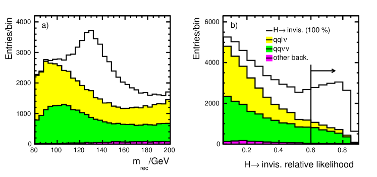
In the limit where the $\mathup{{{H}}}\to\text{invis.}$ branching ratio is small (as expected), the expected uncertainty on the number of invisible Higgs decays selected by a particular likelihood cut is driven by the statistical fluctuations on the number of background events, $\sqrt{B}$. In this limit, the corresponding uncertainty on the cross section for $\mathup{{{H}}}\mathup{{{Z}}}$ production with $\mathup{{{H}}}\to\text{invis.}$ is given by

$$\Delta\sigma_{\text{invis.}}=\frac{\sqrt{B}}{S}\sigma_{\mathup{{{H}}}\mathup{{{Z}}}}^{\rm SM}\,,$$

where $S$ is the number of signal events that would have been selected for the case of a 100 % branching fraction for $\mathup{{{H}}}\to\text{invis.}$ This uncertainty is minimised for a relative likelihood cut of ${\cal{L}}>0.60$, resulting in a $\pm 0.58\,\%$ statistical uncertainty on a $\sigma_{\text{invis.}}$, relative to the SM cross section for $\mathup{{{\mathup{{{e}}}}}^{\scriptstyle{+}}}\mathup{{{\mathup{{{e}}}}}^{\scriptstyle{-}}}\to\mathup{{{H}}}\mathup{{{Z}}}$. The corresponding selection efficiencies are shown in Tab. 4, where the expected background from SM $\mathup{{{H}}}\mathup{{{Z}}}$ production includes the $\mathup{{{H}}}\to\mathup{{{Z}}}\mathup{{{Z}}}^{*}\to\mathup{}\mathup{{\overline{{\upnu}}}}\mathup{}\mathup{{\overline{{\upnu}}}}$ component that has a SM branching fraction of 0.1 %.

Process	$\sigma/\text{fb}$	$\varepsilon_{\text{presel}}$	$\varepsilon^{\text{invis.}}_{{\cal{L}}>0.60}$	$N_{{\cal{L}}>0.60}$
$\mathup{{{q}}}\mathup{{\overline{{\mathup{{{q}}}}}}}\ell\mathup{}$	5914	0.9 %	0.03 %	951
$\mathup{{{q}}}\mathup{{\overline{{\mathup{{{q}}}}}}}\mathup{}\mathup{{\overline{{\upnu}}}}$	325	14.8 %	1.83 %	2985
$\mathup{{{H}}}\mathup{{{\mathup{}}}{}_{\scriptstyle{\!\mathup{{{e}}}}}}\mathup{{\overline{{\mathup{}}}}{}_{\scriptstyle{\!\mathup{{{e}}}}}}$	52	5.6 %	0.37 %	95
$\mathup{{{H}}}\mathup{{{Z}}}$; $\mathup{{{Z}}}\to\mathup{{{q}}}\mathup{{\overline{{\mathup{{{q}}}}}}}$	93	0.2 %	0.06 %	31
$\mathup{{{H}}}\to\text{invis.}$   (100 %)	[93]	48.6 %	23.52 %	10983

Table 4: Summary of the CLIC $(\mathup{{{H}}}\rightarrow\text{invis.})(\mathup{{{Z}}}\rightarrow\mathup{{{q}}}\mathup{{\overline{{\mathup{{{q}}}}}}})$ event selection at $\sqrt{s}=350\,\text{GeV}$, giving the raw cross sections, preselection efficiency, overall selection efficiency for a likelihood cut of ${\cal{L}}>0.60$ and the expected numbers of events passing the event selection for an integrated luminosity of $500\,\text{fb}^{-1}$ and unpolarised electron and positron beams. The numbers shown for the invisible Higgs decay modes correspond to a 100 % branching ratio.

A more optimal approach to extracting the signal cross section is to fit the shape of the likelihood distribution of Fig. 8b, rather than simply imposing a single likelihood cut. In the limit that the invisible branching ratio is small, the resulting Gaussian uncertainty on the $\mathup{{{H}}}\mathup{{{Z}}}$ production cross section with invisible Higgs decays is

$$\frac{\Delta\sigma_{\text{invis.}}}{\sigma_{\mathup{{{H}}}\mathup{{{Z}}}}^{\rm SM}}=\pm 0.56\,\%\,,$$

relative to the SM $\mathup{{{\mathup{{{e}}}}}^{\scriptstyle{+}}}\mathup{{{\mathup{{{e}}}}}^{\scriptstyle{-}}}\to\mathup{{{H}}}\mathup{{{Z}}}$ cross section. For the SM Higgs, the corresponding expected 90 % confidence level upper limit on the invisible Higgs branching ratio is

$$\text{BR}(\mathup{{{H}}}\to\text{invis.})<0.94\,\%\ \ \text{at}\ 90\,\%\ \text{C.L.}$$

3.6 Model independence of the hadronic recoil mass measurement

By combining the two analyses for $\mathup{{{H}}}\mathup{{{Z}}}$ production where $\mathup{{{Z}}}\to\mathup{{{q}}}\mathup{{\overline{{\mathup{{{q}}}}}}}$ and the Higgs decays either to visible or invisible final states,

$$\sigma(\mathup{{{H}}}\mathup{{{Z}}})=\frac{\sigma_{\text{vis.}}+\sigma_{\text{invis.}}}{\text{BR}(\mathup{{{Z}}}\to\mathup{{{q}}}\mathup{{\overline{{\mathup{{{q}}}}}}})}\,,$$

it is possible to determine the absolute $\mathup{{{\mathup{{{e}}}}}^{\scriptstyle{+}}}\mathup{{{\mathup{{{e}}}}}^{\scriptstyle{-}}}\to\mathup{{{H}}}\mathup{{{Z}}}$ cross section in a nearly model-independent manner. Since the fractional uncertainties (relative to the total cross section) on the visible and invisible cross sections are 1.7 % and 0.6 % respectively, the fractional uncertainty on the total cross section will be the quadrature sum of these two fractional uncertainties, namely

$$\Delta\sigma(\mathup{{{H}}}\mathup{{{Z}}})=\pm 1.8\,\%\,.$$

Thus, the Higgsstrahlung cross section can be measured with a precision of better than 2 % at $\sqrt{s}=350\,\text{GeV}$ using the hadronic recoil mass (with unpolarised beams). Such a measurement is competitive with that obtainable from the leptonic recoil mass measurement at $\sqrt{s}=250\,\text{GeV}$, where a precision of $\pm 2.6\,\%$bib:ILC_Physics_TDR is achievable with 250 $\text{fb}^{-1}$ of data (assuming $-80\,\%$ and $+30\,\%$ polarisation of the electron and positron beams). The strongest physics argument for operating a linear collider at $\sqrt{s}=250\,\text{GeV}$ is the model-independent measurement of $\sigma(\mathup{{{H}}}\mathup{{{Z}}})$ that provides a determination of $g_{\mathup{{{H}}}\mathup{{{Z}}}\mathup{{{Z}}}}$. If it can be argued that the hadronic recoil mass measurement is effectively independent of the nature of the Higgs boson decay modes (including possible extensions to the SM), then the arguments for operating an $\mathup{{{\mathup{{{e}}}}}^{\scriptstyle{+}}}\mathup{{{\mathup{{{e}}}}}^{\scriptstyle{-}}}$ linear collider at $\sqrt{s}\sim 250\,\text{GeV}$ are greatly reduced; almost all other measurements of the properties of the Higgs boson are found to benefit from higher centre-of-mass energies bib:ILC_Physics_TDR . In addition, operating at $\sqrt{s}\sim 350\,\text{GeV}$ allows the study of Higgs production through the $\mathup{{{W}}}\mathup{{{W}}}$-fusion process and the pair production of top quarks.

However, the hadronic recoil mass measurement of $\sigma(\mathup{{{H}}}\mathup{{{Z}}})$ can only be truly model independent if the overall (visible + invisible) selection efficiency is independent of the Higgs decay mode. Tab. 5 summarises the combined selection efficiency for $\mathup{{{\mathup{{{e}}}}}^{\scriptstyle{+}}}\mathup{{{\mathup{{{e}}}}}^{\scriptstyle{-}}}\to\mathup{{{H}}}\mathup{{{Z}}}(\mathup{{{Z}}}\to\mathup{{{q}}}\mathup{{\overline{{\mathup{{{q}}}}}}})$, broken down into the different Higgs decay modes. Also shown are the efficiency for $\mathup{{{H}}}\to\mathup{{{W}}}\mathup{{{W}}}^{*}$ decays broken down into the different $\mathup{{{W}}}$ decay modes, covering a very wide range of event topologies, from four-jet final states $(\mathup{{{q}}}\mathup{{\overline{{\mathup{{{q}}}}}}}\mathup{{{q}}}\mathup{{\overline{{\mathup{{{q}}}}}}})$ to final states with two relatively soft particles, for example the visible tau decay products from $\mathup{{{W}}}\mathup{{{W}}}^{*}\to\mathup{}\mathup{}\mathup{}\mathup{}$. For all final-state topologies, the combined (visible + invisible) selection efficiency lies between 19 % and 26 % compated to the mean selection efficiency of $\sim 23\,\%$; a relative variation of $\pm 15\,\%$. It should be noted that these numbers are only indicative, since the measured cross sections are extracted from fits to the likelihood distributions, rather than from a selection imposing hard cuts.

Decay mode	$\varepsilon^{\text{vis.}}_{{\cal{L}}>0.65}$	$\varepsilon^{\text{invis.}}_{{\cal{L}}>0.60}$	$\varepsilon^{\text{vis.}}+\varepsilon^{\text{invis.}}$
$\mathup{{{H}}}\to\text{invis.}$	<0.1 %	23.5 %	23.5 %
$\mathup{{{H}}}\to\mathup{{{q}}}\mathup{{\overline{{\mathup{{{q}}}}}}}/\mathup{{{g}}}\mathup{{{g}}}$	22.6 %	<0.1 %	22.6 %
$\mathup{{{H}}}\to\mathup{{{W}}}\mathup{{{W}}}^{*}$	22.1 %	0.1 %	22.2 %
$\mathup{{{H}}}\to\mathup{{{Z}}}\mathup{{{Z}}}^{*}$	20.6 %	1.1 %	21.7 %
$\mathup{{{H}}}\to\mathup{{}^{\scriptstyle{+}}}\mathup{{}^{\scriptstyle{-}}}$	25.3 %	0.2 %	25.5 %
$\mathup{{{H}}}\to\mathup{}\mathup{}$	25.7 %	<0.1 %	25.7 %
$\mathup{{{H}}}\to\mathup{{{Z}}}\mathup{}$	18.6 %	0.3 %	18.9 %
$\mathup{{{H}}}\to\mathup{{{W}}}\mathup{{{W}}}^{*}\rightarrow\mathup{{{q}}}\mathup{{\overline{{\mathup{{{q}}}}}}}\mathup{{{q}}}\mathup{{\overline{{\mathup{{{q}}}}}}}$	20.8 %	<0.1 %	20.8 %
$\mathup{{{H}}}\to\mathup{{{W}}}\mathup{{{W}}}^{*}\rightarrow\mathup{{{q}}}\mathup{{\overline{{\mathup{{{q}}}}}}}\ell\mathup{}$	23.3 %	<0.1 %	23.3 %
$\mathup{{{H}}}\to\mathup{{{W}}}\mathup{{{W}}}^{*}\rightarrow\mathup{{{q}}}\mathup{{\overline{{\mathup{{{q}}}}}}}\mathup{}\mathup{}$	23.1 %	<0.1 %	23.1 %
$\mathup{{{H}}}\to\mathup{{{W}}}\mathup{{{W}}}^{*}\rightarrow\ell\mathup{}\ell\mathup{}$	26.5 %	0.1 %	26.5 %
$\mathup{{{H}}}\to\mathup{{{W}}}\mathup{{{W}}}^{*}\rightarrow\ell\mathup{}\mathup{}\mathup{}$	21.1 %	0.5 %	21.6 %
$\mathup{{{H}}}\to\mathup{{{W}}}\mathup{{{W}}}^{*}\rightarrow\mathup{}\mathup{}\mathup{}\mathup{}$	16.3 %	2.3 %	18.7 %

Table 5: Summary of the efficiencies of the $\mathup{{{H}}}(\mathup{{{Z}}}\rightarrow\mathup{{{q}}}\mathup{{\overline{{\mathup{{{q}}}}}}})$ analyses at $\sqrt{s}=350\,\text{GeV}$, giving the overall selection efficiency for the visible analysis (${\cal{L}}>0.65$) and the invisible Higgs analysis (${\cal{L}}>0.60$). Here $\ell$ refers to either $\mathup{{{e}}}$ or .

Decay mode	$\Delta$(BR)	$\sigma^{\text{vis.}}+\sigma^{\text{invis.}}$ Bias
$\mathup{{{H}}}\to\text{invis.}$	$+5\,\%$	$-0.01\,\%$
$\mathup{{{H}}}\to\mathup{{{q}}}\mathup{{\overline{{\mathup{{{q}}}}}}}$	$+5\,\%$	$+0.05\,\%$
$\mathup{{{H}}}\to\mathup{{{W}}}\mathup{{{W}}}^{*}$	$+5\,\%$	$-0.18\,\%$
$\mathup{{{H}}}\to\mathup{{{Z}}}\mathup{{{Z}}}^{*}$	$+5\,\%$	$-0.30\,\%$
$\mathup{{{H}}}\to\mathup{{}^{\scriptstyle{+}}}\mathup{{}^{\scriptstyle{-}}}$	$+5\,\%$	$+0.60\,\%$
$\mathup{{{H}}}\to\mathup{}\mathup{}$	$+5\,\%$	$+0.79\,\%$
$\mathup{{{H}}}\to\mathup{{{Z}}}\mathup{}$	$+5\,\%$	$-0.74\,\%$
$\mathup{{{H}}}\to\mathup{{{W}}}\mathup{{{W}}}^{*}\rightarrow\mathup{}\mathup{}\mathup{}\mathup{}$	$+5\,\%$	$-0.98\,\%$

Table 6: Biases in the extracted $\mathup{{{H}}}(\mathup{{{Z}}}\rightarrow\mathup{{{q}}}\mathup{{\overline{{\mathup{{{q}}}}}}})$ cross section for cases where the Higgs BR to a specific final state is increased by 5 %, i.e. $\text{BR}(\mathup{{{H}}}\to X)\rightarrow\text{BR}(\mathup{{{H}}}\to X)+0.05$.

To assess the impact of the different sensitivities to the different $\mathup{{{H}}}$ decay topologies, the different Higgs decay modes in the $\mathup{{{H}}}\mathup{{{Z}}}$ MC samples are reweighted to correspond to modified (non-SM) branching fractions and the total (visible + invisible) cross section is extracted as before (assuming the SM Higgs branching ratios). Tab. 6 shows the resulting biases in the extracted total cross section for the case when a $\text{BR}(\mathup{{{H}}}\to X)\rightarrow\text{BR}(\mathup{{{H}}}\to X)+0.05$. In all cases, the resulting biases in the extracted total $\mathup{{{H}}}\mathup{{{Z}}}$ cross section are less than 1 %, which should be compared to the 1.8 % statistical uncertainty. These variations represent large deviations from the SM which would be observable in studies of exclusive final states. For example, for an integrated luminosity of 500 $\text{fb}^{-1}$, a 5 % (absolute) increase in branching ratio would result in an increase of 3350 $\mathup{{{H}}}\mathup{{{Z}}}$ events in that particular Higgs decay topology, including an increase of 230 events with either $\mathup{{{Z}}}\to\mathup{{}^{\scriptstyle{+}}}\mathup{{}^{\scriptstyle{-}}}$ and $\mathup{{{Z}}}\to\mathup{{{\mathup{{{e}}}}}^{\scriptstyle{+}}}\mathup{{{\mathup{{{e}}}}}^{\scriptstyle{-}}}$ decays. Such large effects would be observable at a linear collider either through their impact on exclusive Higgs branching ratio analyses or they would manifest themselves as large excesses of events in the event samples obtained from the $\mathup{{{Z}}}\to\mathup{{{\mathup{{{e}}}}}^{\scriptstyle{+}}}\mathup{{{\mathup{{{e}}}}}^{\scriptstyle{-}}}/\mathup{{}^{\scriptstyle{+}}}\mathup{{}^{\scriptstyle{-}}}$ recoil mass analysis. It is therefore reasonable to conclude that unless very large BSM effects had been previously discovered, the hadronic recoil mass study gives an effectively model-independent measurement of the $\mathup{{{H}}}\mathup{{{Z}}}(\mathup{{{Z}}}\rightarrow\mathup{{{q}}}\mathup{{\overline{{\mathup{{{q}}}}}}})$ cross section.

4 The Hadronic Recoil Mass Measurement at the ILC

The hadronic recoil mass study presented in this paper was first performed in the context of the CLIC accelerator, where the first stage of the machine was assumed to operate at $\sqrt{s}=350\,\text{GeV}$. The study was then repeated for the ILC at $\sqrt{s}=350\,\text{GeV}$. Again a full Geant4 simulation of the detector response and a full reconstruction of the simulated events was performed. Since both studies used the same simulation and reconstruction software, only small differences in precisions on $\sigma(\mathup{{{H}}}\mathup{{{Z}}})$ from the hadronic recoil mass measurement at the ILC and CLIC are expected. There are two main effects. Firstly, because of the smaller beam spot at CLIC, the impact of beamstrahlung is greater than for the ILC, leading to a larger number of events towards lower values of $\sqrt{s}^{\prime}$ at CLIC compared to the ILC, where $\sqrt{s}^{\prime}$ is the effective centre-of-mass energy of the colliding electron and positron after the radiation of beamstrahlung photons, although the difference is not large at $\sqrt{s}=350\,\text{GeV}$. Secondly, the ILD detector concept used for the ILC studies has more complete calorimeter coverage down to low polar angles than the CLIC_ILD detector concept used for the CLIC studies. Both effects will tend to degrade the hadronic recoil mass reconstruction for the CLIC configuration compared to the ILC. However, the impact is not large, as can be seen from Fig. 9.

Figure 9: The reconstructed hadronic recoil mass distributions for events passing the preselection cuts a) for the clear two-jet topology of the invisible Higgs decay analysis and b) for the visible Higgs decay analysis. In both cases the distributions compare the CLIC and ILC simulations for $500\,\text{fb}^{-1}$ at $\sqrt{s}=350\,\text{GeV}$, with unpolarised beams.

	${P}(\mathup{{{e}}}^{-},\mathup{{{e}}}^{+})$	$\Delta\sigma_{\text{vis.}}$	$\Delta\sigma_{\text{invis.}}$	$\Delta\,\sigma(\mathup{{{H}}}\mathup{{{Z}}})$
CLIC 500 $\text{fb}^{-1}$ ​​​​	0, 0	$\pm 1.71\,\%$	$\pm 0.56\,\%$	$\pm 1.80\,\%$
ILC    500 $\text{fb}^{-1}$ ​​​​	0, 0	$\pm 1.57\,\%$	$\pm 0.48\,\%$	$\pm 1.63\,\%$
ILC    350 $\text{fb}^{-1}$ ​​​​	$-0.8,+0.3$	$\pm 1.68\,\%$	$\pm 0.52\,\%$	$\pm 1.76\,\%$

Table 7: Summary of the statistical precision achievable on $\sigma(\mathup{{{H}}}\mathup{{{Z}}})$ from the hadronic recoil mass analysis at $\sqrt{s}=350\,\text{GeV}$ for CLIC and the ILC. The ILC numbers are shown for both zero and the nominal beam polarisations.

Tab. 7 compares the statistical precision achievable at a centre-of-mass energy of $\sqrt{s}=350\,\text{GeV}$ for: 500 $\text{fb}^{-1}$ at CLIC with unpolarised beams; 500 $\text{fb}^{-1}$ at the ILC with unpolarised beams; and 350 $\text{fb}^{-1}$ at the ILC with the nominal ILC beam polarisations of $P(\mathup{{{e}}}^{-},\mathup{{{e}}}^{+})=(-0.8,+0.3)$. For the same integrated luminosity and unpolarised beams, the precision achievable at the ILC is approximately 8 % better than that at CLIC, reflecting the slightly better recoil mass resolution at the ILC seen in Fig. 9. Since the instantaneous luminosity at the ILC is expected to scale with the Lorentz boost of the colliding beams $\gamma_{\mathup{{{e}}}}$, the time taken to accumulate 350 $\text{fb}^{-1}$ of data at $\sqrt{s}$ is comparable to the time required for 250 $\text{fb}^{-1}$ at $\sqrt{s}=250\,\text{GeV}$. Hence, for the nominal ILC beam polarisation of $P(\mathup{{{e}}}^{-},\mathup{{{e}}}^{+})=(-0.8,+0.3)$, the statistical precision of $1.8\,\%$ achievable on the $\mathup{{{H}}}\mathup{{{Z}}}$ cross section at $\sqrt{s}=350\,\text{GeV}$ using $\mathup{{{Z}}}\to\mathup{{{q}}}\mathup{{\overline{{\mathup{{{q}}}}}}}$ is directly comparable to the statistical precision of 2.6 % bib:ILC_Physics_TDR ; bib:ILD_LOI ; bib:Li achievable with $250\,\text{fb}^{-1}$ of data at $\sqrt{s}=250\,\text{GeV}$ using $\mathup{{{Z}}}\to\mathup{{{\ell}}^{\scriptstyle{+}}}\mathup{{{\ell}}^{\scriptstyle{-}}}$ decays. This conclusion weakens the motivation for operating a future linear collider significantly below the top-pair production threshold.

5 Centre-of-mass Energy Dependence of the Hadronic Recoil Mass Analysis

Figure 10: The two-dimensional distributions of the reconstructed $\mathup{{{Z}}}$ mass, $m_{\mathup{{{q}}}\mathup{{\overline{{\mathup{{{q}}}}}}}}$, versus the reconstructed hadronic recoil mass, $m_{\mathrm{rec}}$, in the visible Higgs decay analysis, broken down into $\mathup{{{H}}}\mathup{{{Z}}}(\mathup{{{Z}}}\to\mathup{{{q}}}\mathup{{\overline{{\mathup{{{q}}}}}}})$ signal and the SM background for CLIC operating at $\sqrt{s}=250\,\text{GeV}$, $\sqrt{s}=350\,\text{GeV}$ and $\sqrt{s}=420\,\text{GeV}$. All events passing the preselection cuts are included.

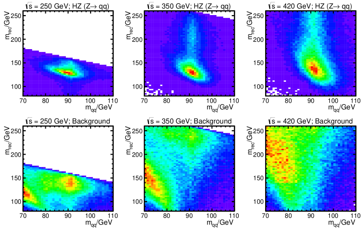
The hadronic recoil mass analysis described above for $\sqrt{s}=350\,\text{GeV}$ was repeated for CLIC at $\sqrt{s}=250\,\text{GeV}$ and $\sqrt{s}=420\,\text{GeV}$. In each case a full set of SM model background processes was generated using the Geant4 simulation of the CLIC_ILD detector concept. Because the complete simulation of the CLIC beam is not available for these centre-of-mass energies; the 250 GeV samples used that same $\sqrt{s^{\prime}}/\sqrt{s}$ distribution as for $\sqrt{s}=350\,\text{GeV}$, whereas the 420 GeV used the $\sqrt{s^{\prime}}/\sqrt{s}$ for the 500 GeV option for CLIC. The analysis described in Sect. 3 was repeated at each centre-of-mass energy using the appropriate distributions for the likelihood function. The binning and range used for $m_{\mathrm{rec}}$ in the two-dimensional distribution of $m_{\mathup{{{q}}}\mathup{{\overline{{\mathup{{{q}}}}}}}}$ versus $m_{\mathrm{rec}}$ was optimized for each centre-of-mass energy. The resulting sensitivities are listed in Tab. 8. Compared to $\sqrt{s}=350\,\text{GeV}$, the overall sensitivity for $\Delta\sigma(\mathup{{{H}}}\mathup{{{Z}}})$ is worse at both $\sqrt{s}=250\,\text{GeV}$ and $\sqrt{s}=420\,\text{GeV}$, although for two different reasons (explained below).

Machine	$\sqrt{s}$	$\cal{L}$	$\sigma(\mathup{{{H}}}\mathup{{{Z}}})$	$\Delta\sigma_{\text{vis.}}$	$\Delta\sigma_{\text{invis.}}$	$\Delta\,\sigma(\mathup{{{H}}}\mathup{{{Z}}})$
CLIC	250 GeV	500 $\text{fb}^{-1}$	136 fb	$\pm 3.63\,\%$	$\pm 0.45\,\%$	$\pm 3.65\,\%$
CLIC	350 GeV	500 $\text{fb}^{-1}$	93 fb	$\pm 1.71\,\%$	$\pm 0.56\,\%$	$\pm 1.80\,\%$
CLIC	420 GeV	500 $\text{fb}^{-1}$	68 fb	$\pm 2.42\,\%$	$\pm 1.02\,\%$	$\pm 2.63\,\%$

Table 8: Summary of the statistical precision achievable on $\sigma(\mathup{{{H}}}\mathup{{{Z}}})$ from the hadronic recoil mass analysis at CLIC for $\sqrt{s}=250\,\text{GeV}$, $\sqrt{s}=350\,\text{GeV}$ and $\sqrt{s}=420\,\text{GeV}$. In each case unpolarised beams were assumed.

Fig. 10 shows two-dimensional distributions of $m_{\mathup{{{q}}}\mathup{{\overline{{\mathup{{{q}}}}}}}}$ versus $m_{\mathrm{rec}}$, broken down into signal and background for the three centre-of-mass energies considered. Sect. 3.3. For all centre-of-mass energies, the most significant backgrounds are from $\mathup{{{\mathup{{{e}}}}}^{\scriptstyle{+}}}\mathup{{{\mathup{{{e}}}}}^{\scriptstyle{-}}}\to\mathup{{{q}}}\mathup{{\overline{{\mathup{{{q}}}}}}}\mathup{{{q}}}\mathup{{\overline{{\mathup{{{q}}}}}}}$ and $\mathup{{{\mathup{{{e}}}}}^{\scriptstyle{+}}}\mathup{{{\mathup{{{e}}}}}^{\scriptstyle{-}}}\to\mathup{{{q}}}\mathup{{\overline{{\mathup{{{q}}}}}}}\ell\mathup{}$. The $\mathup{{{q}}}\mathup{{\overline{{\mathup{{{q}}}}}}}\ell\mathup{}$ background (predominately from $\mathup{{{\mathup{{{e}}}}}^{\scriptstyle{+}}}\mathup{{{\mathup{{{e}}}}}^{\scriptstyle{-}}}\to\mathup{{{W}}}\mathup{{{W}}}$) accounts for the broad band of events on the left-hand side of the background plots. This event population is well separated from the signal region. The more significant background arises from the $\mathup{{{q}}}\mathup{{\overline{{\mathup{{{q}}}}}}}\mathup{{{q}}}\mathup{{\overline{{\mathup{{{q}}}}}}}$ final state, populating the regions with $m_{\mathup{{{q}}}\mathup{{\overline{{\mathup{{{q}}}}}}}}\sim m_{\mathup{{{Z}}}}$. In this region, the $\mathup{{{q}}}\mathup{{\overline{{\mathup{{{q}}}}}}}\mathup{{{q}}}\mathup{{\overline{{\mathup{{{q}}}}}}}$ background arises primarily from $\mathup{{{\mathup{{{e}}}}}^{\scriptstyle{+}}}\mathup{{{\mathup{{{e}}}}}^{\scriptstyle{-}}}\to\mathup{{{W}}}\mathup{{{W}}}$, $\mathup{{{\mathup{{{e}}}}}^{\scriptstyle{+}}}\mathup{{{\mathup{{{e}}}}}^{\scriptstyle{-}}}\to\mathup{{{Z}}}\mathup{{{Z}}}^{*}$ and $\mathup{{{\mathup{{{e}}}}}^{\scriptstyle{+}}}\mathup{{{\mathup{{{e}}}}}^{\scriptstyle{-}}}\rightarrow\mathup{{{Z}}}\mathup{}^{*}$, where the “$*$” indicates an off-mass-shell particle; the component from $\mathup{{{\mathup{{{e}}}}}^{\scriptstyle{+}}}\mathup{{{\mathup{{{e}}}}}^{\scriptstyle{-}}}\rightarrow\mathup{{{Z}}}\mathup{{{Z}}}$, where both $\mathup{{{Z}}}$ bosons are on-shell is largely suppressed by the preselection cuts. The board recoil mass distribution for the preselected $\mathup{{{q}}}\mathup{{\overline{{\mathup{{{q}}}}}}}\mathup{{{q}}}\mathup{{\overline{{\mathup{{{q}}}}}}}$ background is pushed towards the kinematic limit due to two main effects: i) the pair of jets with the invariant mass closest to $m_{\mathup{{{Z}}}}$ is used to calculate the four-momentum of the assumed $\mathup{{{Z}}}$ boson, in the case of the $\mathup{{{\mathup{{{e}}}}}^{\scriptstyle{+}}}\mathup{{{\mathup{{{e}}}}}^{\scriptstyle{-}}}\to\mathup{{{W}}}\mathup{{{W}}}\to\mathup{{{q}}}\mathup{{\overline{{\mathup{{{q}}}}}}}\mathup{{{q}}}\mathup{{\overline{{\mathup{{{q}}}}}}}$ background, this can lead to pairing of two jets from different $\mathup{{{W}}}$-boson decays; ii) for events with significant ISR or beamstrahlung, the calculated recoil mass (which uses the assumed centre-of-mass energy $\sqrt{s}$, rather than $\sqrt{s^{\prime}}$) is higher than the invariant mass of the recoiling system.

From Fig. 10 it can be clearly seen that the width of the recoil mass distribution for $\mathup{{{H}}}\mathup{{{Z}}}(\mathup{{{Z}}}\to\mathup{{{q}}}\mathup{{\overline{{\mathup{{{q}}}}}}})$ events increases with increasing centre-of-mass energy. This can be understood from the expression for the recoil mass:

$$m^{2}_{\text{rec}} =(\sqrt{s}-E_{\mathup{{{Z}}}})^{2}-(-\vec{p}_{\mathup{{{Z}}}})^{2}$$

$$=s-2\sqrt{s}\,E_{\mathup{{{Z}}}}+E_{\mathup{{{Z}}}}^{2}-\vec{p}_{\mathup{{{Z}}}}^{2}$$

$$\approx s+m_{\mathup{{{Z}}}}^{2}-2\sqrt{s}\,(E_{1}+E_{2})\,,$$

where $E_{1}$ and $E_{2}$ are the energies of the two jets forming the reconstructed $\mathup{{{Z}}}$ boson and assuming $E_{\mathup{{{Z}}}}^{2}-\vec{p}_{\mathup{{{Z}}}}^{2}\approx m_{\mathup{{{Z}}}}^{2}$, which is true for the signal region. Propagating the errors on the jet energy measurements, $\sigma_{1}$ and $\sigma_{2}$, implies that

$$\sigma_{m_{\text{rec}}} =\frac{\sqrt{s}}{m_{\text{rec}}}\,\left(\sigma_{1}^{2}+\sigma_{2}^{2}\right)^{\frac{1}{2}}\,.$$

Therefore, the recoil mass resolution is expected to worsen with increasing centre-of-mass energy due to both the $\sqrt{s}$ dependence and the fact that the absolute uncertainty on the jet energies increases with jet energy ($\sigma_{E}\sim 0.03E$) and therefore with centre-of-mass energy. The increasing width of the recoil mass distribution accounts for the increase of $\Delta\sigma_{\text{invis.}}$ with $\sqrt{s}$, listed in Tab. 8, and the larger value of $\Delta\sigma_{\text{vis.}}$ at $\sqrt{s}=420\,\text{GeV}$. However, despite the better recoil mass resolution, the sensitivity to $\Delta\sigma_{\text{vis.}}$ at $\sqrt{s}=250\,\text{GeV}$ is significantly worse than for the other centre-of-mass energies considered. The reason for this can be seen clearly in Fig. 10. At $\sqrt{s}=250\,\text{GeV}$, $\mathup{{{H}}}\mathup{{{Z}}}$ production is not very far above threshold and the recoil mass distribution is relatively close to the kinematic limit. This is the region populated by the large $\mathup{{{q}}}\mathup{{\overline{{\mathup{{{q}}}}}}}\mathup{{{q}}}\mathup{{\overline{{\mathup{{{q}}}}}}}$ background passing the preselection cuts, resulting in a greatly reduced separation between signal and background in the variable that provides the best distinguishing power, namely $m_{\mathrm{rec}}$.

6 Summary and Conclusions

This paper presents the first detailed study of the potential of the hadronic recoil mass analysis at a future linear collider, both for visible Higgs decay modes and possible BSM invisible decay modes. By combining the analyses for visible and invisible modes, it is shown that the measured $\mathup{{{\mathup{{{e}}}}}^{\scriptstyle{+}}}\mathup{{{\mathup{{{e}}}}}^{\scriptstyle{-}}}\to\mathup{{{H}}}\mathup{{{Z}}}(\mathup{{{Z}}}\to\mathup{{{q}}}\mathup{{\overline{{\mathup{{{q}}}}}}})$ cross section does not depend strongly on the nature of the Higgs boson decay and thus provides a model-independent determination of $g_{\mathup{{{H}}}\mathup{{{Z}}}\mathup{{{Z}}}}$. The statistical precision achievable at CLIC operating at $\sqrt{s}=350\,\text{GeV}$ with $500\,\text{fb}^{-1}$ of data with unpolarised beams is $\Delta\sigma_{\mathup{{{H}}}\mathup{{{Z}}}}\approx\pm 1.8\,\%$. A similar precision is obtained for the ILC with $350\,\text{fb}^{-1}$ and the nominal beam polarisation of $P(\mathup{{{e}}}^{+},\mathup{{{e}}}^{-})=(+30\,\%,-80\,\%)$. In both cases the branching ratio to invisible decay modes can be constrained to $\text{BR}(\mathup{{{H}}}\to\text{invis.})<1\,\%$ at 90 % confidence level. It is demonstrated that $\sqrt{s}=350\,\text{GeV}$ is likely to be close to the optimal energy for the hadronic recoil mass analysis; at lower centre-of-mass energies there is less discrimination between signal and background and at higher centre-of-mass energies the measurement is limited by the worsening recoil mass resolution.

It is often stated that operation of a future $\mathup{{{\mathup{{{e}}}}}^{\scriptstyle{+}}}\mathup{{{\mathup{{{e}}}}}^{\scriptstyle{-}}}$ linear collider close to threshold ($\sqrt{s}\sim 250\,\text{GeV}$) is necessary to provide an absolute measurement of the coupling between the Higgs boson and the $Z$ boson, $g_{\mathup{{{H}}}\mathup{{{Z}}}\mathup{{{Z}}}}$. This is based on the determination of $g_{\mathup{{{H}}}\mathup{{{Z}}}\mathup{{{Z}}}}$ from the recoil mass analysis for $\mathup{{{\mathup{{{e}}}}}^{\scriptstyle{+}}}\mathup{{{\mathup{{{e}}}}}^{\scriptstyle{-}}}\to\mathup{{{H}}}\mathup{{{Z}}}(\mathup{{{Z}}}\to\mathup{{{\ell}}^{\scriptstyle{+}}}\mathup{{{\ell}}^{\scriptstyle{-}}})$. The results presented in this paper show that, for a comparable running time, a statistically more precise measurement can be obtained from $\mathup{{{\mathup{{{e}}}}}^{\scriptstyle{+}}}\mathup{{{\mathup{{{e}}}}}^{\scriptstyle{-}}}\to\mathup{{{H}}}\mathup{{{Z}}}(\mathup{{{Z}}}\to\mathup{{{q}}}\mathup{{\overline{{\mathup{{{q}}}}}}})$ events at $\sqrt{s}=350\,\text{GeV}$. This conclusion argues against initial operation of a future linear collider at significantly below the top-pair production threshold.

References

- (1) M. Aicheler et al., A Multi-TeV Linear Collider based on CLIC Technology: CLIC Conceptual Design Report (2012), CERN-2012-007.
- (2) T. Behnke et al., The International Linear Collider Technical Design Report – Volume 1: Executive Summary, ILC-REPORT-2013-040 (2013).
- (3) S. Dawson, et al., Higgs Working Group Report of the Snowmass 2013 Community Planning Study, arXiv:1310.8361v2.
- (4) R. S. Gupta, H. Rzehak and J. D. Wells, How well do we need to measure the Higgs boson couplings?, Phys. Rev. D86 (2012) 095001.
- (5) H. Baer et al., The International Linear Collider Technical Design Report – Volume 2: Physics, ILC-REPORT-2013-040 (2013), arXiv:1306.6352.
- (6) H. Abramowicz, et al., Physics at the CLIC Linear Collider – Input to the Snowmass process, (2013), arXiv:1307.5288v3.
- (7) W. Kilian, T. Ohl, J. Reuter, WHIZARD: Simulating Multi-Particle Processes at LHC and ILC, Eur. Phys. J. C71 (2011) 1742.
- (8) T. Behnke, et al., The International Large Detector: Letter of Intent (2010), arXiv:1006.3396.
- (9) H. Li, Impacts of SB2009 on the Higgs Recoil Mass Measurement Based on a Fast Simulation Algorithm for the ILD Detector, (2010), arXiv:1007.3008.
- (10) M. A. Thomson, Particle Flow Calorimetry and the PandoraPFA Algortithm, Nucl. Instrum. Meth. A611 (2009) 25.
- (11) A. Miyamoto, A measurement of the total cross section of at a future collider using the hadronic decay node of the (2013), arXiv:1311.2248v1.
- (12) S. Agostinelli, et al., Geant4 - A Simulation Toolkit,Nucl. Instrum. Meth. A506 (2003) 250.
- (13) J. Allison, K. Amako, J. Apostolakis, H. Araujo, P. Dubois, et al., Geant4 Developments and Applications, IEEE Trans. Nucl.Sci. 53 (2006) 270.
- (14) L. Linssen, A. Miyamoto, M. Stanitzki and H. Weerts (eds.), Physics and Detectors at CLIC: CLIC Conceptual Design Report, (2012), CERN-2012-003, arXiv:1202.5940.
- (15) T. Sjostrand, S. Mrenna, P. Z. Skands, Pythia 6.4 Physics and Manual, JHEP 0605 (2006) 026.
- (16) I. G. Knowles and G. D. Lafferty, Hadronization in Z0 decay, J. Phys. G23 (1997) 731.
- (17) Z. Was, TAUOLA the library for tau lepton decay, and KKMC/KORALB/KORALZ/… status report, Nucl. Phys. Proc. Suppl. 98 (2001) 96.
- (18) S. Dittmaier, C. Mariotti, G. Passarino, R. Tanaka, et al., Handbook of LHC Cross Sections: 2. Differential Distributions,CERN-2012-002, arXiv:1201.3084.
- (19) P. Mora de Freitas and H. Videau, Detector simulation with Mokka/Geant4: present and future, in International Workshop on Linear Colliders (LCWS 2002), Jeju Island, Korea (2002) pp. 623–627.
- (20) F. Gaede, MARLIN and LLCD: Software tools for the ILC, Nucl. Instrum. Meth. A559 (2006) 177.
- (21) J. S. Marshall, A. Münnich and M. A. Thomson, Performance of Particle Flow Calorimetry at CLIC, Nucl. Instrum. Meth. A700 (2013) 153.
- (22) M. Cacciari, G. P. Salam, G. Soyez, FastJet user manual, Eur. Phys. J. C72 (2012) 1896.