Using pulse shape analysis to improve the position resolution of a resisitive anode microchannel plate detector

Abstract

Digital signal processing techniques were employed to investigate the joint use of charge division and risetime analyses for the resistive anode (RA) coupled to a microchannel plate detector (MCP). In contrast to the typical approach of using the relative charge at each corner of the RA, this joint approach results in a significantly improved position resolution. A conventional charge division analysis utilizing analog signal processing provides a position measured resolution of 170 $\mu$m (FWHM). By using the correlation between risetime and position we were able to obtain a measured resolution of 92 $\mu$m (FWHM), corresponding to an intrinsic resolution of 64 $\mu$m (FMHM) for a single Z-stack MCP detector.

1 Introduction

Position-sensitive microchannel plate (MCP) detectors are a powerful and widely used tool in imaging of electrons, photons and ions [1]. Since their inception in the late 1950’s [2], they have been used in a variety of applications ranging from ion-molecule reaction scattering experiments [3] to fast neutron radiography [4]. In this detector, an incident electron, photon, or ion ejects an electron from the micorchannel plate. The microchannel plate acts as a continuous dynode electron multiplier with millions of independent channels providing a typical amplification of $\approx$10³. Two MCP plates (chevron configuration) or three plates (Z-stack configuration) can be stacked to achieve higher gains. Different methods exist for measuring the position of the electron cloud exiting the microchannel plate thus determining the position of the incident particle. The principal techniques are : multi-anode [5], helical delay line [6], induced signal [7], and resistive anode [8]. The resistive anode (RA) technique is particularly appealing for its simplicity. The electron cloud emanating from the MCP stack is incident on a two-dimensional resistive sheet. Readout of the charge at the four corners of the sheet provides a measure of position of the incident particle via charge centroiding. Utilizing this simple approach a position resolution of 134 $\mu$m (FWHM) for a chevron configuration has been achieved [9]. Although for many application a chevron stack of two microchannel plates provides sufficient amplification, the detection of low-intensity signals near the one electron limit requires configurations involving three (Z-stack) or more MCPs. For a Z-stack configuration the best reported resolution is 100-200 $\mu$m (FWHM) [10]. By use of more complex MCP stack configurations and through the use of retarding potentials, position resolution as good as 50 $\mu$m (FWHM) has been realized [11, 12, 13]. In this work, we investigate the use of pulse shape analysis to improve the position resolution obtained with a simple Z-stack MCP-RA detector.

2 Experimental setup

Depicted in Fig. 1 is the experimental setup used to determine the position resolution of the MCP-RA detector. Alpha particles from a ²⁴¹Am radioactive source (A) are emitted towards a secondary electron emission foil (C). Electrons are emitted by the passage of an $\alpha$ particle through the 1.5 $\mu$m thick aluminized mylar foil. Ejected electrons are accelerated to an energy of $\approx$ 1.3 keV by the potential difference between the aluminized foil and a wire grid (D). The electrons then pass through slits in a stainless steel mask (E) directly in front of the microchannel plate stack (F) before impinging on the front surface of the MCP-RA detector. The precision mask, fabricated by laser micro-machining [14], has ten slits each measuring 100 $\mu$m by 7620 $\mu$m and spaced by either 4.2 or 4.5 mm apart. Electrons that pass through slits in the mask are amplified by the Z-stack MCP and detected on a resistive anode (G). Alpha particles traverse the aluminized mylar foil and are detected by a fast scintillator/photomultiplier tube (PMT) assembly (B) placed directly behind the aluminized foil. The MCP used was a standard Z-stack (APD 3 40/12/10/12 D 60:1) with 10 $\mu$m diameter microchannels provided by Photonis USA [15] which was coupled to a 40 mm diameter RA from Quantar Technology Inc. [16]. Further details of the experimental setup can be found in [17].

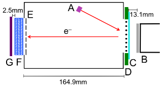
Figure 1: Experimental setup used to measure the position resolution of the Z-stack MCP-RA detector [17]. See text for details.

The entire assembly presented in Fig. 1 is housed in a vacuum chamber that is evacuated to a pressure of 4 x 10^-8 torr. The microchannel plates were biased to a voltage of +3139 V using a ISEG NHQ224M low-noise, high voltage power supply (HVPS). The RA was biased to +3284 V, also using a ISEG NHQ224M HVPS. The secondary electron emission foil and photomultiplier tube were biased to voltages of -300 V and -1800 V using HK 5900 and Bertan 362 HVPS respectively. Signals detected at each corner of the resistive anode were amplified by a high quality charge sensitive amplifier (CSA) [18] operated in vacuum. The four CSAs are situated approximately 13 cm from the MCP-RA to mimimize cable capacitance. The output signals from the CSAs are coupled to a 250 MS/s digitizer (Caen DT5720B) [19]. Readout of the digitizer is triggered by the coincidence of a fast signal extracted from the back of the MCP detector and the PMT. The digitizer is readout by a standard PC and waveforms are recorded for subsequent analysis. For the analysis subsequently described the waveforms associated with a total of 260,000 coincident triggers were recorded.

Indicated in Fig. 2 is the reverse pincushion shape of the resistive anode (black) along with the circular outline of the 40 mm diameter MCP detector (blue). Superimposed on the RA is the image of the ten slits provided by the stainless steel mask (green). The four corners of the MCP-RA are designated Q₁, Q₂, Q₃, and Q₄ as evident in Fig. 2. Along with the relative position of the MCP-RA and mask, shown in Fig. 2 are the signals measured at two locations on the RA. One set of digitized traces (red) correspond to an electron cloud incident at the the bottom slit of the RA as indicated by the red square. The other set of traces (black) correspond to a position close to the center of the RA as indicated by the black square. The waveforms associated with these two positions are markedly different. When the position signal arises from the center of the detector all the waveforms are essentially the same as is expected. However, when the signal originates at the bottom of the RA, while the two corners nearest the signal exhibit a fast risetime followed by an exponential decay, the upper corners of the RA manifest a significantly slower risetime. This risetime, dictated by the RC of the resistive anode thus provides a measure of the particle’s position. Motivated by prior work which utilized the risetime of signals in resistive silicon detectors to achieve position sensitivity in one dimension [20], we elected to characterize the RA waveforms by their risetime. The risetime (RT) of each signal was defined as the time required for the signal to go from 10$\%$ to 90$\%$ of its maximum value. As the slits in the mask are oriented to probe the Y dimension of the RA, for the remainder of this work we focus on the position information in that dimension.

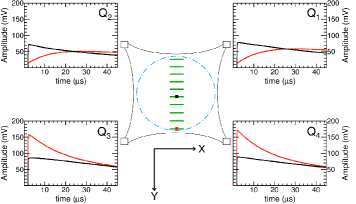
Figure 2: (Color Online) Schematic of the RA (black) along with the outline of the 40 mm diameter MCP (blue) and slits in the stainless steel mask (green). Pulse shapes associated with the electron cloud incident on two locations of the RA are also shown. Slit 0 (s0) corresponds to the bottom slit and slit 9 (s9) to the topmost slit.

3 Signal Risetime analysis

Signals obtained from the CAEN digitizer are processed through a series of mathematical operations using a standard C++ code calling ROOT [21] libraries. In the present investigation the sampling resolution is 4 ns since the digitizer used has a sampling frequency of 250 MS/s. The obtained signals are corrected for the DC offset and gains for different channels for CSA’s on an event-by-event basis.

Presented in Fig. 3 is the correlation between the risetime observed for signals at the two bottom corners if the RA namely Q₃ and Q₄. Given the exponential dependence of the signal amplitude on the RC of the resistive anode, the correlation is examined on a logarithmic scale. Individual slits are clearly evident in Fig. 3 with low numbered slits exhibiting shorter risetimes and higher numbered slits associated with longer risetimes. An overall linear dependence between log(RT_Q3) and log(RT_Q4) is observed as one moves from the bottom of the RA (s0) to the top (s9). Interestingly, a large jump in risetime is observed between slit 5 (s5) and slit 6 (s6), indicating a high sensitivity of the risetime to position in the center of the detector. Moreover, these two slits, in contrast to the other slits manifest a broad range of risetimes in at least one of the two risetimes. Electrons associated with these slits often do not show a strong correlation between the risetime of Q₃ and the risetime of Q₄ as indicated by the horizontal and vertical bands in the figure. Both the large sensitivity to position of the risetime in this region of the detector and the large dispersion in risetime are likely due to the fact that the charge cloud incident in this region experiences near equal resistance in all directions and a relatively small gradient in all directions. For all but these center two slits however the risetime measured for the two corners exhibits a clear anti-correlation. This anti-correlation arises from the spatial extent of each slit in the x dimension. Motivated by the overall positive correlation between log(RT_Q3) and log(RT_Q4) we construct the quantity log(RT_Q3) + log(RT_Q4) corresponding to a line of unity slope in Fig. 3. It is clearly evident that the spacing of the slits along this line is not uniform.

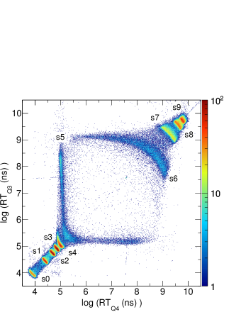
Figure 3: (Color online) Correlation between the risetime extracted from CSA output signals for the corners Q3 and Q4. The numbering of the slits is indicated in the figure.

In Fig.4 the dependence of the summed risetime, log(RT_Q3) + log(RT_Q4), on the position in the Y dimension is explored. The position in the Y dimension is determined by using the charge division method proposed by [5, 8].

$$Y_{position}=(Q_{3}+Q_{4})/Q_{total}$$ (1)

$$Q_{total}=Q_{1}+Q_{2}+Q_{3}+Q_{4}$$ (2)

To obtain the charge measured at each corner of the MCP-RA we have utilized digital filtering techniques to provide signal conditioning. We initially used a gaussian filter on the digitized signal to integrate the signal from each CSA resulting in a gaussian-like pulse. The amplitude of this pulse is related to the charge measured at the corner. To efficiently realize the gaussian filter a recursive algorithm was employed [22, 23]. Use of an integration and differentiation time constant of 500 ns was determined to result in the best position resolution. The resolution obtained is comparable to the resolution of 170 $\mu$m obtained for this experimental setup with analog electronics [17]. To determine the sensitivity of our result to the filtering technique chosen we also used a trapezoidal filter. Further details on the signal processing can be found in the Appendix.

Evident in Fig. 4 is a clear correlation between the summed risetime and the $Y_{position}$ of the electron cloud. Since $Y_{position}$=0 is associated with the top of the RA, as the value of $Y_{position}$ increases one observes a general decrease in the summed risetime. This trend is understandable since as the position of the electron cloud moves closer to the bottom of the RA the risetime decreases as initially evident in Fig. 1. The correlation observed for the upper half of the RA, $Y_{position}$ $<$0.45 is also observed for the lower half of the RA, $Y_{position}$$>$ 0.45. The fact that the observed locus is not centered on $Y_{position}$=0.5 is likely due to the uncertainty in the positioning of the mask relative to the RA. Situated along the locus of points in Fig. 4, that is the main feature of the spectrum, are a series of peaks corresponding to the slits in the mask. An enlarged region centered on slit 3 is displayed in the inset of the figure. The relationship between summed risetime and $Y_{position}$ exhibited by the peaks in 4 provides useful information. It describes how these two quantities should be related for a given position of the electron cloud on the RA. Selection of the data in these peaks corresponds to approximately 25 $\%$ of the data. Aside from the strong locus with peaks visible in Fig. 4 one also observes data that does not lie on this locus. The majority of this data is associated with horizontal lines which originate from one of the ten peaks. Examination of the pulse shapes associated with this data clearly establishes that much of this data is associated with the pileup of two signals. Such a pileup disturbs the baseline for the signal distorting the measured charge while minimally disturbing the signal risetime.

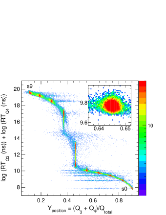
Figure 4: (Color online) Dependence of the summed risetime of Q3 and Q4 on the Y position of the electron cloud. The peaks corresponding to slit 0 (s0) and slit 9 (s9) are indicated. The peak associated with slit 3 is presented in the inset.

To investigate if using the joint information from the summed risetime together with the charge division method provides an improvement in the position resolution we selected the ten peaks visible in Fig. 4. As the resulting distributions are reasonably well described by a gaussians, they were fit with this functional form. As the distance between the slits corresponding to each of the peaks is well known the position spectrum was calibrated and the position resolution extracted. The resulting resolution is presented in Fig. 5.

To begin we examine the measured resolution where only the charge division technique is utilized for the digitized signals. The result for this case which does not make use of any risetime information is presented as the cross symbol (green). The resolution obtained from this analysis with the trapezoidal filter is typically 190 $\mu$m (FWHM). Use of the gaussian filter (not shown) gives a comparable result. As the use of these filters mimics the use of an analog shaping amplifier, also shown for comparison is the resolution obtained from the use of analog electronics. Although the resolution obtained with the analog electronics is $\approx$20 $\mu$m lower than that obtained with the trapezoidal filter it is not a dramatic reduction. Moreover, using the analog electronics a reasonable resolution could only be obtained for the four central slits [17]. In contrast, using the digital signal processing approach a relatively uniform resolution is obtained across the entire detector. The somewhat lower value observed for the two edge slits is due to the slight deviation of the distributions from gaussians.

The measured resolution obtained by the joint use of summed risetime along with charge division is depicted by the red circles (gaussian filter) and blue triangles (trapezoidal filter) respectively. Both filters provide a measured resolution of $\approx$90 $\mu$m across entire detector. This result is a significant improvement over the use of the charge division approach alone. No systematic advantage is observed for one filter as compared to the other filter. Averaging the measured resolution of the central eight slits for either the trapezoidal or gaussian filters, one obtains an average measured resolution of 92 $\mu$m. Accounting for the finite slit width of 100 $\mu$m this measured resolution corresponds to an intrinsic resolution of 64 $\mu$m [17]. This result is competitive with the resolution obtained using more complex MCP arrangements and a retarding potential [11, 12, 13].

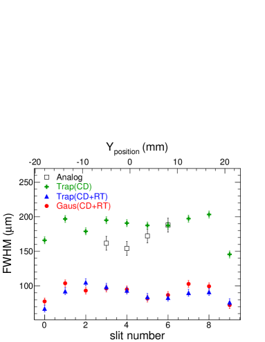
Figure 5: (Color online) Comparison of the measured resolution as a function of slit (position) using the correlation between risetime and position with the charge division approach alone. The resolution obtained using analog electronics is shown for reference.

4 Conclusions

Resistive anode (RA) MCP detectors are widely used to provide position resolution in the detection of electrons, photons, or ions. A charge division approach from the four corners of the RA is typically utilized to extract the centroid of the electron cloud emanating from the MCP. The signals arriving at the four corners of the RA manifest a broad range of risetimes. For a 40 mm diameter MCP-RA detector, risetimes range from $<$ 1$\mu$s to approximately 40 $\mu$s. By digitizing the signals from the MCP-RA with a high speed digitizer, digital signal processing techniques were utilized to extract both the charge collected at each corner as well as the risetime of the four signals for each incident electron. Implementation of the charge division approach resulted in a resolution of $\approx$190 $\mu$m (FWHM), comparable to that obtained with analog electronics. Examination of the digitized signals reveals a clear correlation between the risetime of the signals and the position of the electron cloud. By using this correlation between risetime and position together with the charge division method a measured position resolution of $\approx$90 $\mu$m (FWHM) was achieved, corresponding to an intrinsic resolution of 64 $\mu$m (FWHM). This result represents a significant improvement in the position resolution obtained. It was also observed that in the central region of the detector the risetime is extremely sensitive to the position of the electron cloud. While this latter observation requires further investigation for full characterization, it presents intriguing possibilities for enhanced imaging capabilities.

A key question in image processing is the speed with which signals can be processed. We therefore assessed the rate at which signals could be processed through our implementation of the digital filters described. Using a 2.8 GHz i686 PC we measured a rate of approximately 350 coincident events/s for the trapezoidal filter and 200 events/sec for the gaussian filter. In the near term this processing rate could be increased by parallelization to make use of multiple cores on the computer. A longer term goal would involve implementation of FPGA processing at the detector level to both achieve a high processing rate and reduce the volume of data acquired.

5 Acknowledgments

We gratefully acknowledge the technical support provided by the personnel in the Mechanical Instrument Services and Electronic Instrument Services at the Department of Chemistry, Indiana University. This research is based upon work supported by the U.S. Department of Energy, National Nuclear Security Administration under Award Number DE-NA0002012.

6 Appendix: Signal Processing

Standard digital signal processing techniques are used on the CSA signals to extract the position resolution using gaussian and trapezoidal filter algorithms [22, 24, 25, 26]. To efficiently process the pulse shapes, recursive relations of both the filters were employed. For the gaussian shaper, the input signal is subjected to a combination of high-pass and low-pass filters. Each sample, $i$ of the $j^{th}$ channel CSA is subjected to a single-pole, high-pass digital filter using the following recursive relation [22]

$$HP_{out}^{j}[i]=a_{HP}^{0}CSA^{j}[i]+a_{HP}^{1}CSA^{j}[i-1]$$

$$+b_{HP}^{1}HP_{out}^{j}[i-1]$$ (3)

where $a_{HP}^{0},\mbox{ }a_{HP}^{1},\mbox{ and }b_{HP}^{1}$ are the coefficients of the high-pass filter kernel, which can be calculated from the following equations

$$a_{HP}^{0}=(1+e^{-1/\Delta_{H}})/2$$ (4)

$$a_{HP}^{1}=-(1+e^{-1/\Delta_{H}})/2$$ (5)

$$b_{HP}^{1}=e^{-1/\Delta_{H}}$$ (6)

$\Delta_{H}$ refers to the number of samples being considered for the high-pass time constant. The factor $e^{-1/\Delta_{H}}$ decides the sample-to-sample decay for a given time constant. Equation (3) mimics an analog differentiator circuit whose RC constant can be controlled by using the parameter $\Delta_{H}$ (in the units of number of samples). A time constant of 500 ns was used for all the channels of CSA. Due to finite length of the exponential tail of input signal, the high pass filter output may overshoot the baseline of the pulse. This tendency can be corrected by using a pole-zero recursive relation [23]. We utilized the pole-zero recursive relation given by the following equation

$$HP_{corr}^{j}[i]=HP_{out}^{j}[i]+PZC\times CSA^{j}[i-1]$$ (7)

where $PZC$ is a pole-zero correction factor. The value of $PZC$ can be chosen so as to correct for the overshoot. The second term provides the amplified (attenuated) exponential tail of the input pulse which corrects against the pole present in the exponential part of $HP_{out}^{j}$. The pole-zero corrected output of the high-pass filter is then transformed by a four-pole, low-pass digital filter, which is realized by the following recursive relations [22]

$$GSH^{j}[i]=a_{LP}^{0}HP_{corr}^{j}[i]+b_{LP}^{1}GSH^{j}[i-1]$$ (8)

$$+b_{LP}^{2}GSH^{j}[i-2]+b_{LP}^{3}GSH^{j}[i-3]+b_{LP}^{4}GSH^{j}[i-4]$$

where $a_{LP}^{0},\mbox{ }b_{LP}^{1},\mbox{ }b_{LP}^{2},\mbox{ }b_{LP}^{3},\mbox{ }b_{LP}^{4}$ are the coefficients of a low-pass filter kernel and $GSH^{j}$ refers to the semi-gaussian shaper output obtained for the $j^{th}$ channel. The corresponding coefficients for the low-pass filter is given as

$$a_{LP}^{0}=(1-e^{-1/\Delta_{L}})^{4}$$ (9)

$$b_{LP}^{1}=4e^{-1/\Delta_{L}}$$ (10)

$$b_{LP}^{2}=-6(e^{-1/\Delta_{L}})^{2}$$ (11)

$$b_{LP}^{3}=4(e^{-1/\Delta_{L}})^{3}$$ (12)

$$b_{LP}=-(e^{-1/\Delta_{L}})^{4}$$ (13)

where $\Delta_{L}$ is the low-pass time constant of the high-pass filter. For each corner of the resistive sheet, the measured charge is obtained by determining the height of the semi-gaussian shaper output.

To ensure that the extracted resolution was not limited by the particular filter chosen, we also implemented a trapezoidal digital filter to extract the charge of the input signals. The following recursive relations are used for the $j^{th}$ channel CSA

$$d^{k,j}[i]=CSA^{j}[i]-CSA^{j}[i-k]$$ (14)

$$d^{k,l,j}[i]=d^{k,j}[i]-d^{k,j}[i-l]$$ (15)

$$p^{j}[i]=p^{j}[i-1]+m_{2}d^{k,l,j}[i]$$ (16)

$$r^{j}[i]=p^{j}[i]+m_{1}d^{k,l,j}[i]$$ (17)

$$s^{j}[i]=s^{j}[i-1]+r^{j}[i]$$ (18)

Here $k$ represents the number of samples in the rising edge while $l$ is the total number of samples in the rising as well as in flat top region of the trapezoid shaped signal, $m_{2}$ is the gain of the filter, $m_{1}$ is the pole-zero correction factor, and $s^{j}$ is the output of the filter. The correction factor depends on the decay time constant ($\tau$) of the preamplifier, given by the following equation [25]

$$m_{1}=\frac{m_{2}}{e^{(T_{clk}/\tau)}-1}$$ (19)

where $T_{clk}$ is the sample resolution of the digitizer. For shaping the CSA signals both the rising and flat top lengths are chosen to be 500 ns and the sample resolution is taken to be 4 ns. The gain of the shaper is taken to be unity, while the decay time constant is chosen to be 30 $\mu s$ to match the decay constant of the CSA. Charge collected at each corner of the RA is calculated by taking the average height of the trapezoidal output.

References

- Wiza [1979] J. L. Wiza Nucl. Inst. and Meth. 162 (1979) 587.
- Lampton [1981] M. Lampton Sci. Am. 245 (1981) 62.
- Wester [2014] R. Wester Phys. Chem. Chem. Phys. 16 (2014) 396.
- Tremsin et al. [2011] A. S. Tremsin et al., Nucl. Inst. and Meth. A 652 (2011) 400.
- Fraser [1984] G. W. Fraser, Nucl. Inst. and Meth. A 221 (1984) 115.
- Sobottka and Williams. [1988] S. Sobottka, M. Williams, IEEE Trans. Nucl. Sci. 35 (1988) 348.
- deSouza et al. [2012] R. T. deSouza, Z. Q. Gosser, S. Hudan, Rev. Sci. Instrum. 83 (2012) 053305.
- Lampton and Carlson [1979] M. Lampton, C. W. Carlson, Rev. Sci. Instrum. 50 (1979) 1093.
- Wiza et al. [1979] J. L. Wiza, P. R. Henkel, R. L. Roy, Rev. Sci. Instrum. 48 (1979) 1217.
- Downie et al. [1993] P. Downie et al., Meas. Sci. Technol. 4 (1993) 1293.
- Firmani et al. [1982] C. Firmani, E. Ruiz, C. W. Carlson, M. Lampton, F. Parsece, Rev. Sci.Instrum. 53 (1982) 570.
- Floryan and Johnson. [1989] R. F. Floryan, C. B. Johnson, Rev. Sci. Instrum. 60 (1989) 339.
- Murakami et al. [2010] G. Murakami, K. Yoshioka, I. Yoshikawa, Appl. Opt. 49 (2010) 1293.
- Mic [2015] Potomac Photonics, 2015. URL: http://www.potomac-laser.com.
- Mic [2015] Photonis USA, 2015. URL: http://www.photonis.com.
- Mic [2015] Quantar Technology Inc., 2015. URL: http://www.quantar.com.
- Wiggins et al. [2015] B. B. Wiggins et al., Rev. Sci. Instrum. 86 (2015) 083303.
- Davin et al. [2001] B. Davin et al., Nucl. Inst. and Meth. A 473 (2001) 302.
- Mic [2015] Caen Technologies, Inc., 2015. URL: http://www.caen.it.
- Kalbitzer and Melzer [1967] S. Kalbitzer, W. Melzer, Nucl. Instr. and Meth. 56 (1967) 301.
- R. Brun, and F. Rademakers [1997] R. Brun, F. Redemakers, Nucl. Instr. and Meth. A 399 (1997) 81.
- S. W. Smith [1997] S. W. Smith, The Scientist and Engineer’s Guide to Digital Signal Processing, California Technical Pub; 1st edition ISBN 978-0966017632 (1997) 319.
- Kihm et al. [2003] T. Kihm, V. F, Bobrakov, H. V. Klapdor-Kleingrothaus, Nucl. Inst. and Meth. A 498 (2003) 334.
- V. T. Jordanov, G. F. Knoll [1994] V. T. Jordanov, G. F. Knoll, Nucl. Instr. and Meth. A 345 (1994) 337.
- V. T. Jordanov, G. F. Knoll et al. [1994] V. T. Jordanov, Nucl. Instr. and Meth. A 353 (1994) 261.
- V. Radeka [1972] V. Radeka, Nucl. Instr. and Meth. A 99 (1972) 525.