Unified description of the optical phonon modes in -layer MoTe2
Abstract
-layer transition metal dichalcogenides provide a unique platform to investigate the evolution of the physical properties between the bulk (three dimensional) and monolayer (quasi two-dimensional) limits. Here, using high-resolution micro-Raman spectroscopy, we report a unified experimental description of the -point optical phonons in -layer -molybdenum ditelluride (MoTe2). We observe a series of -dependent low-frequency interlayer shear and breathing modes (below , denoted LSM and LBM) and well-defined Davydov splittings of the mid-frequency modes (in the range , denoted iX and oX), which solely involve displacements of the chalcogen atoms. In contrast, the high-frequency modes (in the range , denoted iMX and oMX), arising from displacements of both the metal and chalcogen atoms, exhibit considerably reduced splittings. The manifold of phonon modes associated with the in-plane and out-of-plane displacements are quantitatively described by a force constant model, including interactions up to the second nearest neighbor and surface effects as fitting parameters. The splittings for the iX and oX modes observed in -layer crystals are directly correlated to the corresponding bulk Davydov splittings between the and modes, respectively, and provide a measurement of the frequencies of the bulk silent and optical phonon modes. Our analysis could readily be generalized to other layered crystals.
Keywords: Two-dimensional materials, layered crystals, transition metal dichalcogenides, MoTe2, Raman spectroscopy, interlayer breathing and shear modes, force constants, Davydov splitting, surface effects.
Introduction In the wake of graphene, a vast family of layered materials is attracting tremendous attention Geim and Grigorieva (2013). Now available in the form of -layer crystals, the latter exhibit peculiar physical properties that complement the assets of graphene and offer exciting perspectives to design van der Waals heterostructures Geim and Grigorieva (2013). Semiconducting transition metal dichalcogenides (MX2, with M = Mo, W and X = S, Se, Te) are among the most actively investigated layered crystals Wilson and Yoffe (1969). Indeed, although bulk MX2 exhibit indirect bandgaps, monolayer MX2 are direct bandgap semiconductors Mak et al. (2010); Splendiani et al. (2010) with remarkable spin, valley Xu et al. (2014) and optoelectronic properties Peng et al. (2015). More Generally, -layer MX2 crystals provide an ideal platform to uncover the impact of symmetry breaking and interlayer interactions on the electronic, optical and vibrational properties, from the bulk (three-dimensional) to the monolayer (quasi two-dimensional) limit.
In particular, in -layer MX2, interlayer interactions result in a splitting of all the monolayer phonon modes Wieting and Verble (1971); Molina-Sánchez and Wirtz (2011); Luo et al. (2013a, b); Terrones et al. (2014); Ribeiro-Soares et al. (2014); Yamamoto et al. (2014); Scheuschner et al. (2015); Zhang et al. (2015); Zhao et al. (2013) (see Table 1). The latter effect is known as the Davydov splitting Davydov (1971) and is closely related to the force constants that govern the vibrational properties of MX2 Luo et al. (2013a). The Davydov splitting has been previously studied in polyaromatic molecules Khelladi (1975), thin films Aroca et al. (1987), and bulk layered crystals, including MX2 Wieting and Verble (1971); Wieting et al. (1980); Ghosh and Maiti (1983); Molina-Sánchez and Wirtz (2011); Luo et al. (2013a). Recently, low-frequency Raman spectroscopy has been employed in -layer MoS2 Plechinger et al. (2012); Zeng et al. (2012); Zhao et al. (2013); Zhang et al. (2013); Boukhicha et al. (2013) and WSe2 Zhang et al. (2013) to uncover the fan diagrams associated with the frequencies of the interlayer shear (LSM) and breathing (LBM) modes, which arise from the Davydov splitting of the zero frequency acoustic modes (see Fig. 1(d)). Related splittings of the higher frequency modes involving intralayer atomic displacements have been reported in -layer MoSe2 Tonndorf et al. (2013); Chen et al. (2015) and WS2 Staiger et al. (2015). Thus far, such splittings have solely been reported for the out-of-plane Raman-active phonon with symmetry in the bulk, whereas other high-frequency modes, such as the in-plane phonon with symmetry in the bulk, exhibit anomalous -dependent frequency shifts Lee et al. (2010); Li et al. (2012); Molina-Sánchez and Wirtz (2011); Luo et al. (2013a, b); Tonndorf et al. (2013); Berkdemir et al. (2013); Yamamoto et al. (2014) but no splitting. However, a unified description of the Davydov splitting in -layer MX2 is still lacking.
In this letter, we quantitatively investigate the Davydov splitting of all the -point optical phonon modes, over the range in -layer molybdenum ditelluride (MoTe2) crystals. As in other MX2, -layer MoTe2 displays a set of (herein () denote the floor (ceil) functions that map to the largest previous (smallest following) integer) well-separated LSM and LBM below . In the range , the in-plane and out-of-plane modes involving solely displacements of the chalcogen (Te) atoms (herein denoted iX and oX) exhibit pronounced splittings into and Raman-active modes, respectively. The Davydov splitting between the bulk in-plane Raman-active and silent modes (out-of-plane Raman-active and silent modes) is (). In the range , the modes involve motion of both the metal (Mo) and chalcogen (Te) atoms. The in-plane iMX mode exhibits no observable splitting. The out-of-plane oMX mode exhibits a small splitting of approximately , which is actually not a Davydov splitting but a splitting due to surface effects.
All the observed trends are fitted using a finite linear chain model that includes inter- and intralayer force constants up to the second nearest neighbor, as well as surface effects at the edges of the chain Luo et al. (2013a). This model naturally explains why the interlayer force constants, which directly determine the manifold of rigid layer modes, also give rise to sizable Davydov splittings for the iX and oX modes but to reduced splittings for the iMX and oMX modes. Conversely, surface effects are responsible for the apparent downshift of the iMX mode as augments and for the slight splitting of the oMX mode.
| Number of | LSM | LBM | iX | oX | iMX | oMX |
| layers | ||||||
| 1 | ||||||
| 2 | ||||||
| odd N | ||||||
| even N | ||||||
| bulk | ||||||
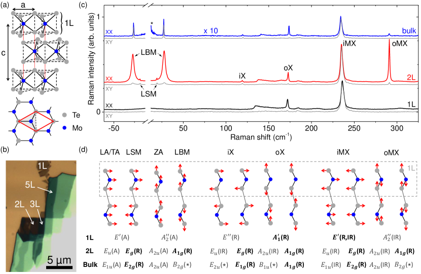
In its stable form, bulk MoTe2 displays a trigonal prismatic ( polytype) structure with AbA/BaB stacking (see Fig. 1) and shares many properties with the widely studied MoS2, MoSe2, WS2 and WSe2 crystals Wilson and Yoffe (1969); Ribeiro-Soares et al. (2014). MoTe2 has recently attracted particular interest due to its lower transport bandgap Fathipour et al. (2014); Lezama et al. (2014); Lin et al. (2014); Pradhan et al. (2014) and near-infrared emission Ruppert et al. (2014); Lezama et al. (2015). Indeed, at room temperature, monolayer MoTe2 exhibits a direct optical bandgap at 1.1 eV, whereas the bulk material has an indirect optical bandgap slightly below 1.0 eV Wilson and Yoffe (1969); Ruppert et al. (2014); Lezama et al. (2015). Bulk MoTe2 exhibits 3 acoustic and 15 optical phonon modes at as is the case for MoS2 and MoSe2 Wieting and Verble (1971); Molina-Sánchez and Wirtz (2011); Luo et al. (2013a); Ribeiro-Soares et al. (2014); Yamamoto et al. (2014); Scheuschner et al. (2015); Zhang et al. (2015); Zhao et al. (2013). As illustrated in Fig 1, the manifold of optical phonons breaks down into 5 (doubly degenerate) in-plane modes and 5 out-of-plane modes. According to group theory Loudon (1964), the integrated intensity of the in-plane Raman-active modes is expected to be independent on the angle between the polarization of the incoming and scattered photons, whereas the integrated intensity of the out-of-plane modes should exhibit a dependence.
Results Figure 1 shows the micro-Raman spectra of monolayer, bilayer and bulk MoTe2 recorded at for (parallel configuration, XX) and (cross-polarized configuration, XY). We first address the low-frequency range below . In bulk MoTe2, we observe only a single feature at that shows similar intensities in the XX and XY configurations. The latter is assigned to the in-plane interlayer shear mode (LSM) with symmetry Wieting et al. (1980). For , we observe a prominent feature at that shows strong extinction in the XY polarization and a fainter feature at whose intensity is similar in the XX and XY configurations. The former is thus assigned to the out-of-plane layer breathing mode (LBM) with symmetry, whereas the latter is assigned to the LSM with symmetry. The LBM has symmetry in the bulk and is silent. As expected, we do not observe any interlayer mode for .
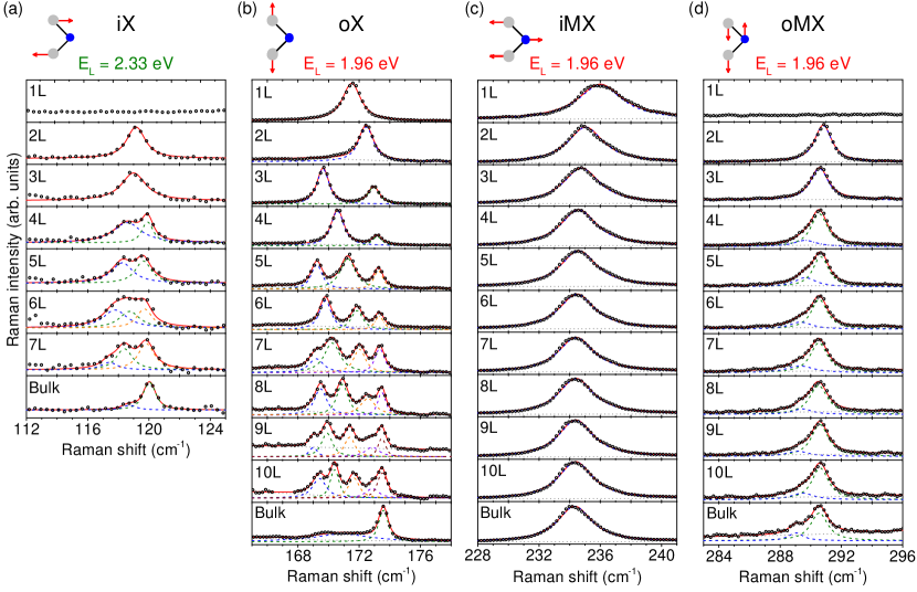
In the mid- and high-frequency ranges, the Raman spectra of bilayer MoTe2 displays four one-phonon features, which have previously been identified as originating from the following intralayer displacements: (i) the in-plane, out-of-phase vibration of the Te planes, with symmetry in the bulk (iX mode, near ), (ii) the out-of-plane, out-of-phase vibration of the Te planes, with symmetry in the bulk (oX mode, near 170 cm-1), (iii) the in-plane vibration of the Mo and Te planes against each other, with symmetry in the bulk (iMX mode, near 230 cm-1), and (iv) the out-of-plane vibration of the Mo and Te planes against each other, with symmetry in the bulk, (oMX mode, near 290 cm-1) Yamamoto et al. (2014); Guo et al. (2015); Wieting et al. (1980). The bulk iX and oMX modes are predicted to be Raman inactive in a backscattering geometry and silent, respectively. However, both modes appear as faint features in thick MoTe2 flakes (considered as a bulk reference). This surprising observation, also reported recently on other MX2 might be a consequence of the finite penetration depth of our laser due to the strong optical absorption of MoTe2 Wilson and Yoffe (1969); Ruppert et al. (2014) or may arise from a breakdown of the Raman selection rules due to resonance effects Luo et al. (2013b); Lee et al. (2015); Scheuschner et al. (2015). As predicted by group theory Ribeiro-Soares et al. (2014); Scheuschner et al. (2015); Yamamoto et al. (2014), the iX and oMX modes are not observed in monolayer MoTe2 (see Figs. 1 and 3(a)). We verified that the oX and oMX features nearly vanish in the XY configuration, whereas the integrated intensities of the iX and iMX features do not change (see Fig. 1).
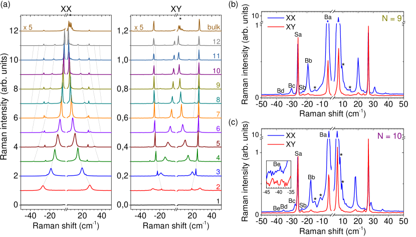
Figure 2 shows the evolution of the low-frequency modes (LSM and LBM) from to -layer MoTe2. As previously reported in multilayer graphene Tan et al. (2012); Lui et al. (2014) and recently in other MX2, Plechinger et al. (2012); Zeng et al. (2012); Zhao et al. (2013); Boukhicha et al. (2013); Zhang et al. (2013); Chen et al. (2015), a set of -dependent low-frequency Stokes and anti-Stokes peaks appears for . The number of detected peaks increases with and the peaks can be separated into branches that seemingly stiffen or soften with increasing (see the dashed lines in Fig 2(a)). Interestingly, compared to a reference recorded in the XX configuration, the integrated intensity of peaks belonging to a branch that softens with increasing drops by more than one order of magnitude in the XY configuration, whereas the integrated intensity of the peaks that belong to a branch that stiffens with increasing is marginally affected. Therefore, the branches that soften (stiffen) with increasing are assigned to the LBM (LSM). We are able to resolve two branches of LSM and, remarkably, five branches of LBM, i.e., the complete manifold of Raman-active LBM up to (see Table 1 and Fig. 5).
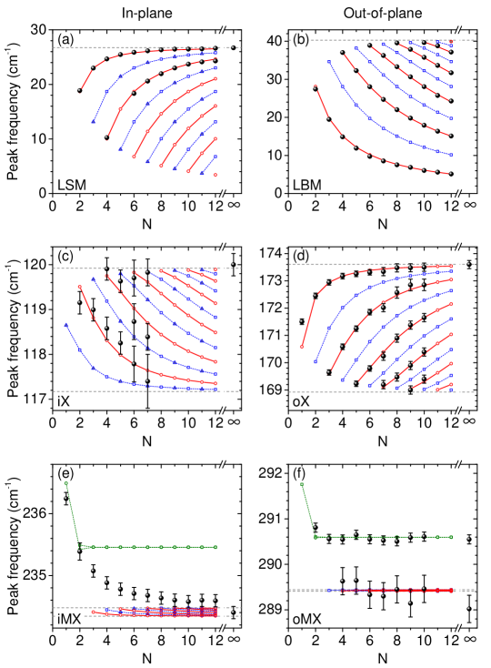
The Raman spectra of the mid- (iX, oX) and high-frequency (iMX and oMX) modes in -layer MoTe2 are shown in Fig. 3. For -layer MoTe2, we observe a prominent splitting of the oX-mode feature (see Fig. 3(b)), whereas in the bulk limit, one recovers a single symmetric feature (assigned to the Raman-active mode). Interestingly, as shown in Fig. 3(a), the iX-mode feature also splits, but only for . We can resolve up to three subfeatures for and 7, but the Raman signal in -layer MoTe2 becomes too small to perform a quantitative analysis. At , the oMX-mode feature also exhibits a modest splitting, on the order of , for . Two subpeaks can be distinguished. However, the evolution of their frequencies does not follow a specific trend as a function of (see Fig. 3(d) and Fig. 5(f)). In contrast, the iMX-mode feature exhibits a faint shoulder on its high-energy side (see Fig. 3(c)), but no appreciable splitting can be resolved. However, the iMX feature downshifts as increases, consistently with previous reports on -layer MX2 Lee et al. (2010); Li et al. (2012); Molina-Sánchez and Wirtz (2011); Luo et al. (2013a, b); Berkdemir et al. (2013); Tonndorf et al. (2013); Zhao et al. (2013); Yamamoto et al. (2014); Ruppert et al. (2014).
The splitting of a bulk phonon mode in a -layer -MX2 can be understood based on a group theory analysis Luo et al. (2013a, b); Terrones et al. (2014); Ribeiro-Soares et al. (2014); Yamamoto et al. (2014); Scheuschner et al. (2015); Staiger et al. (2015); Zhang et al. (2015); Zhao et al. (2013). Bulk MoTe2 belongs to the non-symmorphic space group and crystals with odd or even belong to the and symmorphic space groups, respectively. In bulk -MX2, the (silent) LBM and (Raman active) LSM correspond to an out-of phase displacement of adjacent layer pairs, whereas the iX, iMX, oX, and oMX atomic displacements give rise to two modes, in which the relative motion of equivalent atoms belonging to two adjacent layers is either in-phase or out-of-phase (see Fig. 1(d)). In a -layer system, interlayer interactions and symmetry breaking result in a manifold of LSM and LBM, and iX, oX, iMX and oMX modes. Table 1 summarizes the irreducible representations and the activity of these optical phonon modes for mono-, bi-, -layer, and bulk MoTe2.
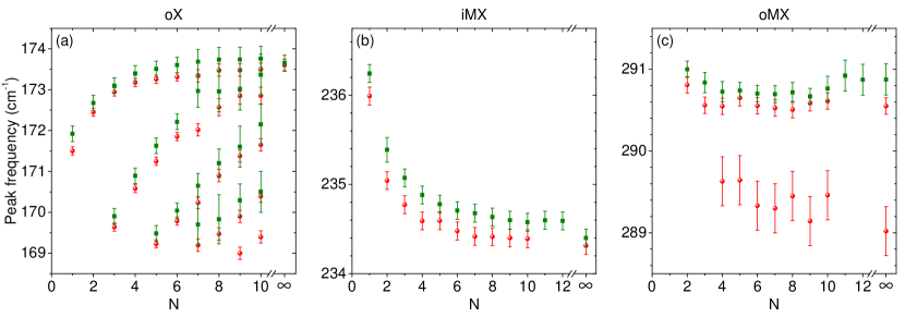
In agreement with group theory predictions, our Raman measurements reveal that (i) secondary LSM and LBM features appear from (ii) the oX feature splits for and we observe Raman active subfeatures in -layer MoTe2, (iii) the splitting of the iX feature into Raman active subfeatures is observed from , (iv) a splitting of the oMX feature appears for . The frequencies of all the measured Raman features, extracted from Voigt fits (see Figs. 2-3) are reported in Fig. 5.
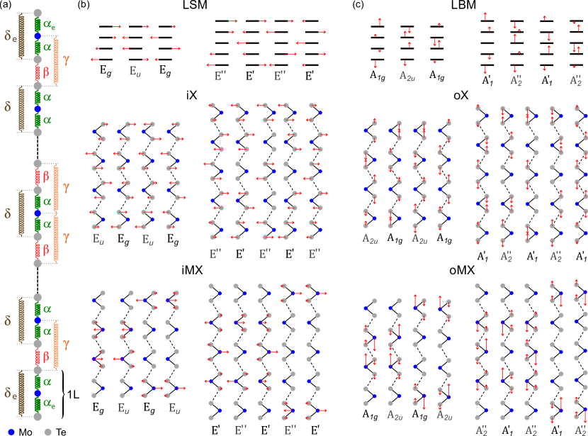
Force constant model We now introduce a semiempirical model to rationalize the observed splittings. -layer MoTe2 is modeled as a finite linear chain composed of Mo atoms and Te atoms. Within one MoTe2 unit nearest neighbor Mo and Te atoms and the pair of second nearest neighbor Te atoms are connected by springs with force constants per unit area and respectively Luo et al. (2013a) (see Fig. 4(a)). Interlayer interactions are then described by two force constants per unit area, and , between nearest neighbor Te atoms belonging to adjacent layers and between second nearest neighbor Mo and Te atoms, respectively. In addition, finite size effects are known to lead to a slight reduction of the metal-chalcogen bond length on the outer layers (“surface effects”) Luo et al. (2013a). As a result, to improve our model, effective values and are phenomenologically considered for the first and layer. We note that our choice of using the same value of at both ends of the chain is consistent with the fact that no significant substrate-induced frequency shifts have been observed on the Raman response of MoTe2 and other MX2 Lee et al. (2010); Yamamoto et al. (2014); Luo et al. (2013a, b); Zhao et al. (2013). The normal modes , with the normal displacement of the atom ( for Te and for Mo) in the MoTe2 layer () associated with the normal mode (see Fig. 4(a)), and the eigenfrequencies of a -layer system can be obtained from Newton’s equations of motion, which lead to the secular equation
| (1) |
involving the dynamical matrix (see Supporting Information).
For in-plane (out-of-plane) displacements, Eq. (1) predicts three manifolds of normal modes that correspond to (i) the low frequency LSM (LBM) (including the zero frequency acoustic mode) (ii) the mid-frequency iX (oX) modes and (iii) the high-frequency iMX (oMX) modes. Figure 4(b) represents the calculated iX and oX normal modes (using the parameters in Table 2) and their irreducible representations for and . For the low- (LSM, LBM) and mid-frequency (iX, oX) modes, the eigenfrequencies increase (decrease) as the layers exhibit more out-of phase (in-phase) relative motion, up to the limit of the highest- (lowest-) frequency mode, which corresponds to an out-of phase (in-phase) oscillation for all layers. This trend is as expected from classical theories of coupled oscillators. In particular, we can readily conclude that the dominant LBM feature corresponds, for even to the out-of-phase oscillation of two blocks composed of layers that vibrate in-phase; for odd to the out-of-phase oscillations of two blocks composed of layers that vibrate in-phase, whereas the central layer stays at rest. In contrast, the dominant LSM feature corresponds to an out-of-phase displacement of adjacent layers as in bulk crystals Michel and Verberck (2012); Zhao et al. (2013) (see also Supporting Information).
As shown in Fig. 5, the fan diagrams associated with the in-plane LSM, iX- and iMX-mode frequencies on the one hand, and out-of-plane LBM, oX- and oMX-mode frequencies on the other hand are very well described by the force-constant model. The force constants (per unit area) used as fitting parameters and the corresponding bulk frequencies (see Supporting Information for their analytical expressions) are reported in Table 2. We find that all the force constants correspond to a restoring force, except for the in-plane second nearest neighbor force constant between Te pairs. The values obtained here are qualitatively similar to the values that Luo et al. reported for MoS2 by fitting the bulk frequencies (obtained from calculations based on the local density approximation (LDA)) to a force constant model Luo et al. (2013a).
| in-plane | out-of-plane | |
| 105 | 159 | |
| 107 | 163 | |
| 2.28 | 5.61 | |
| 0.585 | 1.11 | |
| -4.53 | 19.8 | |
| -4.22 | 20.4 | |
| 26.8 () | 40.3 () | |
| 117.2 | 168.9 | |
| 119.9 | 173.6 |
Discussion First, we note that the low-frequency branches of LSM and LBM can also be separately modeled using a linear chain of -oscillators. Indeed, in first approximation, van der Waals interactions between adjacent layers are sufficient to accurately describe the series of interlayer modes without further consideration of the in-plane crystal structure and intralayer force constants Tan et al. (2012); Michel and Verberck (2012); Zhao et al. (2013); Zhang et al. (2013); Boukhicha et al. (2013). The LSM and LBM frequencies are then very well approximated by , with ( corresponds to the acoustic mode at ). The observed Raman-active modes correspond to branches with (i) for the LSM Sa and Sb and (ii) for the LBM Ba to Be (see Fig. 2 (b),(c)). Using the complete model, the bulk frequencies , with the MoTe2 mass per unit area, then allow to determine effective interlayer force constants per unit area of and for the LSM and LBM, respectively (see Table 2). These values are close to those derived from the LBM and LSM in MoS2 Zhao et al. (2013); Zhang et al. (2013); Boukhicha et al. (2013) and WSe2 Zhao et al. (2013). We note that surface effects only affect intralayer force constants and have therefore a negligible influence on the rigid layer modes.
Second, a force constant model restricted to the first nearest neighbor interactions (i.e., ) suffices to fit the frequencies of the low- and mid-frequency modes, but would then fail to predict the frequencies of the oMX and iMX modes. Indeed, Table 2 reveals that the second nearest neighbor interlayer () and intralayer () force constants are of the same order of magnitude and larger than the nearest neighbor interlayer force constant , respectively. Using the complete model, the bulk Davydov splittings of the iX and oX modes can conveniently be expressed as , with the chalcogen (Te) mass per unit area, leading to the values of and for the iX and oX modes, respectively (see Supporting Information).
According to our calculations and to group theory Ribeiro-Soares et al. (2014); Staiger et al. (2015); Scheuschner et al. (2015) (see Fig. 1,4 and Table 1), the mid-frequency Raman-active modes that are observable in our backscattering experiments correspond (i) to the second-lowest, fourth-lowest,…frequency mode for the iX phonons and (ii) to the highest, third-highest…frequency mode for the oX phonons. These distinct symmetry properties result in a set of softening and stiffening branches in the experimentally measured fan diagrams in Fig. 5(c) and 5(d), respectively. A remarkable validation of this symmetry analysis is that the highest frequency iX mode that can be observed has the highest frequency ( symmetry) for even and the second highest frequency ( symmetry) for odd . As a result, the iX-mode frequency for is lower than for , and the two observed iX-mode subfeatures for are slightly upshifted relative to their counterparts recorded for (see Figs. 3 and 5). We also note that our model predicts a somewhat lower frequency for the oX () mode in monolayer MoTe2 (see Fig. 5(e)). This discrepancy is due to a stronger bond length contraction in the limit of a monolayer Luo et al. (2013a), as compared to the bilayer or to the outer layers in -layer samples.
Third, we focus on the high-frequency iMX and oMX modes. Our model predicts very small anomalous Davydov splittings (below ) for the iMX and oMX modes (consistent with previous studies of the iMX mode in bulk MX2 Wieting et al. (1980); Ghosh and Maiti (1983); Molina-Sánchez and Wirtz (2011); Luo et al. (2013a)) and a critical influence of surface effects. Indeed we find that among the iMX and oMX normal displacements, two modes predominantly involve atomic displacement of the first and/or layer and can be regarded as surface modes. Such surface modes are not predicted for the iX and oX displacements (see Fig. 4 and the Supporting Information). As a result, the surface terms and , will only bring a small correction to the fan diagrams associated with the mid-frequency modes, but will shape the manifold of high-frequency phonon modes. For , our model predicts a fan diagram for quasi-degenerate iMX and oMX modes, where atomic displacement chiefly occurs in the inner layers and two surface modes (see Fig. 4(b) and Fig. 5(c),(f). The strength of the surface effects will set the frequencies of the surface modes relative to that of the other modes.
A tentative explanation for the pronounced downshift observed for the iMX mode is then that the surface mode dominates for small and that the modes arising from the inner layers provide most of the Raman intensity as increases. This scenario is consistent with calculations based on a bond polarizability model Umari et al. (2001), which was also recently used for layered BN and BN nanotubes Wirtz et al. (2005) and which is explained in the Supporting Information. The model predicts that the surface mode will dominate in the iMX peak for . Let us also note that the iMX-mode feature in -layer MoTe2 is appreciably broader (with a full width at half maximum (FWHM) decreasing from 3.5 cm-1 for down to 2.6 cm-1 in the bulk) than the iX, oX and oMX peaks, whose FWHM are approximately 1 cm-1. This broadening prevents us from unveiling any splitting of the iMX-mode feature in -layer MoTe2. This splitting, according to our force-constant fit is very small anyway (see Fig. 5 (e)) and also our ab-initio calculations for phonons of bulk MoTe2 yield a minimal anomalous Davydov splitting of 0.1 cm-1 (see Supporting Information).
For the oMX mode, we also find that the surface modes have a slightly higher frequency than the modes that are localized on the inner layer. Supported by the results from our bond-polarizability model (see Supporting Information), we assign the dominant high-frequency oMX subfeature to the surface mode, while the faint lower-frequency shoulder is assigned to the inner modes. We note that the low-frequency shoulder is not observed at all at (see Supporting Information) and may thus arise from a resonance effect Luo et al. (2013b); Scheuschner et al. (2015); Lee et al. (2015). We also point out that ab-initio calculations (see Supporting Information) yield a sizable Davydov splitting of 5.8 cm-1 between the bulk and frequencies (in the absence of the Lydanne-Sachs-Teller interaction). In order to reproduce this splitting, an additional force-constant between Mo atoms of neighboring layers would need to be introduced (which would not modify the splitting between the oX modes and modes because those modes do not involve motion of the Mo atoms). Since the resulting fan-diagram is not visible in our experimental spectra of the oMX mode – due to almost vanishing intensity – we did not include this additional force constant here.
Finally, we comment on the possible influence of resonance effects on our measurements. Resonance effects should not impact the phonon frequencies but may strongly alter the integrated intensity of one given Raman feature and the repartition of the spectral weight within a given subfeature. For the iX mode, our bond polarizability model predicts spectral weights that are in-line with group theory predictions and our experimental results (see Supporting Information). However, the same model predicts that the highest frequency oX mode should have a much larger oscillator strength than its lower frequency counterparts. This prediction is clearly in contradiction with our observations at (see Fig 3b), where the oX-mode subfeatures have comparable integrated intensities, but is consistent with the absence of splittings seen in numerous studies on MoS2 using visible photon energies Lee et al. (2010); Li et al. (2012); Luo et al. (2013a); Lee et al. (2015); Zhang et al. (2015). Noteworthy, a pronounced splitting of the oX feature was also observed at (see Supporting Information). However, in this case the high-frequency peak largely dominates the oX-mode feature for . These intriguing observations, together with the observation of the iX and oMX bulk modes, and a particularly intense oX-mode feature in monoloayer MoTe2 at (see Supporting Information and Ref. Ruppert et al. (2014)) provide a strong impetus for a quantitative analysis of resonant, symmetry-dependent exciton-phonon coupling Chakraborty et al. (2013); Luo et al. (2013b); Carvalho et al. (2015); Scheuschner et al. (2015); Lee et al. (2015) in -layer MX2.
Conclusion Using micro-Raman spectroscopy, we have reported a unified description of the optical phonon modes in a -layer -transition metal dichalcogenide crystal (here, MoTe2), between the bulk (three-dimensional) and monolayer (quasi-two-dimensional) limits. The manifolds of low-frequency interlayer shear and breathing modes, and of the mid-frequency modes involving out-of-phase intralayer motion of the chalcogen atoms are well understood using classical theories of coupled oscillators. In contrast, the behavior of the high-frequency modes that involve out-of phase motion of the metal and chalcogen planes is largely influenced by surface effects. We have introduced a global fitting procedure based on a linear chain model to derive the force constants up to the second nearest neighbor and to assess the strength of the surface effects. This model allows us to deduce the frequency of optical phonons that are silent in bulk crystals, namely the low-frequency interlayer breathing mode (LBM) with symmetry, and the mid-frequency in-plane (iX) and out-of-plane (oX) modes with and symmetry, respectively (see Table 2). Finally, our work may motivate related studies of Davydov splitting, force constants and surface effects in other layered crystals, such as black phosphorus Favron et al. (2015), bismuth selenide and bismuth telluride Zhao et al. (2014).
Methods -layer MoTe2 crystals were prepared by mechanical exfoliation of commercially available bulk crystals (2D semiconductors) onto Si wafers covered with a 90-nm or 285-nm-thick SiO2 epilayer. The number of layers was first estimated from optical contrast and atomic force microscopy measurements, and further characterized using a home-built micro-Raman setup. Micro-Raman scattering studies were carried out in ambient conditions, in a backscattering geometry using using a monochromator equipped with a 2400 grooves/mm holographic grating, coupled to a two-dimensional liquid nitrogen cooled charge-coupled device (CCD) array. Two laser photon energies ( and were employed. Spectral resolutions of and were obtained at , , respectively. A laser intensity below was used in order to avoid photoinduced damage of our samples. In order to attain the low-frequency range (for measurements at ), a combination of one narrow bandpass filter and two narrow notch filters (Optigrate) was used. After optimization, Raman features at frequencies as low as 4.5 cm-1 could be measured. Polarized Raman studies are performed using a Glan-Thomson analyzer placed before the entrance of our spectrometer. An achromatic half-wave plate was placed after the analyzer and adequately rotated such that the Raman backscattered beam enters the spectrometer with a fixed polarization. Thereafter, we will be considering parallel (XX) and perpendicular (XY) polarizations of the incoming and Raman-scattered photons. The observation of residual features from the out of plane modes (LBM, oX, oMX) in the XY configuration (see Figs. 1 and. 2 is due to depolarization effects induced by our high numerical aperture objective (100 x, ). Finally, the measured Raman features are fit to Voigt profiles, taking into account our spectral resolution.
Acknowledgments We are grateful to C. Faugeras and K. Nogajewski for discussions. We acknowledge financial support from the Agence Nationale de la Recherche (under grant QuanDoGra 12 JS10-001-01), from the CNRS and from Université de Strasbourg, as well as support by the National Research Fund, Luxembourg (projects INTER/ANR/13/20/NANOTMD and C14/MS/7731521/FAST-2DMAT).
References
- Geim and Grigorieva (2013) A. K. Geim and I. V. Grigorieva, Nature 499, 419 (2013).
- Wilson and Yoffe (1969) J. Wilson and A. Yoffe, Advances in Physics 18, 193 (1969).
- Mak et al. (2010) K. F. Mak, C. Lee, J. Hone, J. Shan, and T. F. Heinz, Physical Review Letters 105, 136805 (2010).
- Splendiani et al. (2010) A. Splendiani, L. Sun, Y. Zhang, T. Li, J. Kim, C.-Y. Chim, G. Galli, and F. Wang, Nano Letters 10, 1271 (2010).
- Xu et al. (2014) X. Xu, W. Yao, D. Xiao, and T. F. Heinz, Nature Physics 10, 343 (2014).
- Peng et al. (2015) B. Peng, P. K. Ang, and K. P. Loh, Nano Today 10, 128 (2015).
- Wieting and Verble (1971) T. J. Wieting and J. L. Verble, Phys. Rev. B 3, 4286 (1971).
- Molina-Sánchez and Wirtz (2011) A. Molina-Sánchez and L. Wirtz, Physical Review B 84, 155413 (2011).
- Luo et al. (2013a) X. Luo, Y. Zhao, J. Zhang, Q. Xiong, and S. Y. Quek, Phys. Rev. B 88, 075320 (2013a).
- Luo et al. (2013b) X. Luo, Y. Zhao, J. Zhang, M. Toh, C. Kloc, Q. Xiong, and S. Y. Quek, Phys. Rev. B 88, 195313 (2013b).
- Terrones et al. (2014) H. Terrones, E. D. Corro, S. Feng, J. M. Poumirol, D. Rhodes, D. Smirnov, N. R. Pradhan, Z. Lin, M. a. T. Nguyen, A. L. Elías, T. E. Mallouk, L. Balicas, M. A. Pimenta, and M. Terrones, Scientific Reports 4 (2014), 10.1038/srep04215.
- Ribeiro-Soares et al. (2014) J. Ribeiro-Soares, R. M. Almeida, E. B. Barros, P. T. Araujo, M. S. Dresselhaus, L. G. Cançado, and A. Jorio, Physical Review B 90, 115438 (2014).
- Yamamoto et al. (2014) M. Yamamoto, S. T. Wang, M. Ni, Y.-F. Lin, S.-L. Li, S. Aikawa, W.-B. Jian, K. Ueno, K. Wakabayashi, and K. Tsukagoshi, ACS Nano 8, 3895 (2014).
- Scheuschner et al. (2015) N. Scheuschner, R. Gillen, M. Staiger, and J. Maultzsch, Phys. Rev. B 91, 235409 (2015).
- Zhang et al. (2015) X. Zhang, X.-F. Qiao, W. Shi, J.-B. Wu, D.-S. Jiang, and P.-H. Tan, Chem. Soc. Rev. 44, 2757 (2015).
- Zhao et al. (2013) Y. Zhao, X. Luo, H. Li, J. Zhang, P. T. Araujo, C. K. Gan, J. Wu, H. Zhang, S. Y. Quek, M. S. Dresselhaus, and Q. Xiong, Nano Letters 13, 1007 (2013).
- Davydov (1971) A. S. Davydov, in Theory of Molecular Excitons (Springer US, 1971).
- Khelladi (1975) F. Z. Khelladi, Chemical Physics Letters 34, 490 (1975).
- Aroca et al. (1987) R. Aroca, C. Jennings, R. O. Loutfy, and A.-M. Hor, Spectrochimica Acta Part A: Molecular Spectroscopy 43, 725 (1987).
- Wieting et al. (1980) T. J. Wieting, A. Grisel, and F. Lévy, Physica B+C 99, 337 (1980).
- Ghosh and Maiti (1983) P. N. Ghosh and C. R. Maiti, Phys. Rev. B 28, 2237 (1983).
- Plechinger et al. (2012) G. Plechinger, S. Heydrich, J. Eroms, D. Weiss, C. Schüller, and T. Korn, Applied Physics Letters 101, 101906 (2012).
- Zeng et al. (2012) H. Zeng, B. Zhu, K. Liu, J. Fan, X. Cui, and Q. M. Zhang, Physical Review B 86, 241301 (2012).
- Zhang et al. (2013) X. Zhang, W. P. Han, J. B. Wu, S. Milana, Y. Lu, Q. Q. Li, A. C. Ferrari, and P. H. Tan, Phys. Rev. B 87, 115413 (2013).
- Boukhicha et al. (2013) M. Boukhicha, M. Calandra, M.-A. Measson, O. Lancry, and A. Shukla, Phys. Rev. B 87, 195316 (2013).
- Tonndorf et al. (2013) P. Tonndorf, R. Schmidt, P. Böttger, X. Zhang, J. Börner, A. Liebig, M. Albrecht, C. Kloc, O. Gordan, D. R. T. Zahn, S. Michaelis de Vasconcellos, and R. Bratschitsch, Opt. Express 21, 4908 (2013).
- Chen et al. (2015) S.-Y. Chen, C. Zheng, M. S. Fuhrer, and J. Yan, Nano Letters , 2526 (2015).
- Staiger et al. (2015) M. Staiger, R. Gillen, N. Scheuschner, O. Ochedowski, F. Kampmann, M. Schleberger, C. Thomsen, and J. Maultzsch, Phys. Rev. B 91, 195419 (2015).
- Lee et al. (2010) C. Lee, H. Yan, L. E. Brus, T. F. Heinz, J. Hone, and S. Ryu, ACS Nano 4, 2695 (2010).
- Li et al. (2012) H. Li, Q. Zhang, C. C. R. Yap, B. K. Tay, T. H. T. Edwin, A. Olivier, and D. Baillargeat, Advanced Functional Materials 22, 1385 (2012).
- Berkdemir et al. (2013) A. Berkdemir, H. R. Gutiérrez, A. R. Botello-Méndez, N. Perea-López, A. L. Elías, C.-I. Chia, B. Wang, V. H. Crespi, F. López-Urías, J.-C. Charlier, et al., Scientific reports 3 (2013), 10.1038/srep01755.
- Loudon (1964) R. Loudon, Advances in Physics 13, 423 (1964).
- Fathipour et al. (2014) S. Fathipour, N. Ma, W. S. Hwang, V. Protasenko, S. Vishwanath, H. G. Xing, H. Xu, D. Jena, J. Appenzeller, and A. Seabaugh, Applied Physics Letters 105, 192101 (2014).
- Lezama et al. (2014) I. G. Lezama, A. Ubaldini, M. Longobardi, E. Giannini, C. Renner, A. B. Kuzmenko, and A. F. Morpurgo, 2D Materials 1, 021002 (2014).
- Lin et al. (2014) Y.-F. Lin, Y. Xu, S.-T. Wang, S.-L. Li, M. Yamamoto, A. Aparecido-Ferreira, W. Li, H. Sun, S. Nakaharai, W.-B. Jian, K. Ueno, and K. Tsukagoshi, Advanced Materials 26, 3263 (2014).
- Pradhan et al. (2014) N. R. Pradhan, D. Rhodes, S. Feng, Y. Xin, S. Memaran, B.-H. Moon, H. Terrones, M. Terrones, and L. Balicas, ACS Nano 8, 5911 (2014).
- Ruppert et al. (2014) C. Ruppert, O. B. Aslan, and T. F. Heinz, Nano Letters 14, 6231 (2014).
- Lezama et al. (2015) I. G. Lezama, A. Arora, A. Ubaldini, C. Barreteau, E. Giannini, M. Potemski, and A. F. Morpurgo, Nano Lett. 15, 2336 (2015).
- Guo et al. (2015) H. Guo, T. Yang, M. Yamamoto, L. Zhou, R. Ishikawa, K. Ueno, K. Tsukagoshi, Z. Zhang, M. S. Dresselhaus, and R. Saito, Phys. Rev. B 91, 205415 (2015).
- Lee et al. (2015) J.-U. Lee, J. Park, Y.-W. Son, and H. Cheong, Nanoscale 7, 3229 (2015).
- Tan et al. (2012) P. H. Tan, W. P. Han, W. J. Zhao, Z. H. Wu, K. Chang, H. Wang, Y. F. Wang, N. Bonini, N. Marzari, and N. Pugno, Nature materials 11, 294 (2012).
- Lui et al. (2014) C. H. Lui, Z. Ye, C. Keiser, X. Xiao, and R. He, Nano Letters 14, 4615 (2014).
- Michel and Verberck (2012) K. H. Michel and B. Verberck, Physical Review B 85, 094303 (2012).
- Umari et al. (2001) P. Umari, A. Pasquarello, and A. Dal Corso, Phys. Rev. B 63, 094305 (2001).
- Wirtz et al. (2005) L. Wirtz, M. Lazzeri, F. Mauri, and A. Rubio, Phys. Rev. B 71, 241402 (2005).
- Chakraborty et al. (2013) B. Chakraborty, H. S. S. R. Matte, A. K. Sood, and C. N. R. Rao, Journal of Raman Spectroscopy 44, 92 (2013).
- Carvalho et al. (2015) B. R. Carvalho, L. M. Malard, J. M. Alves, C. Fantini, and M. A. Pimenta, Phys. Rev. Lett. 114, 136403 (2015).
- Favron et al. (2015) A. Favron, E. Gaufrès, F. Fossard, A.-L. Phaneuf-L’Heureux, N. Y. Tang, P. L. Lévesque, A. Loiseau, R. Leonelli, S. Francoeur, and R. Martel, Nature materials (2015), doi:10.1038/nmat4299.
- Zhao et al. (2014) Y. Zhao, X. Luo, J. Zhang, J. Wu, X. Bai, M. Wang, J. Jia, H. Peng, Z. Liu, S. Y. Quek, and Q. Xiong, Phys. Rev. B 90, 245428 (2014).
- Baroni et al. (2001) S. Baroni, S. de Gironcoli, A. Dal Corso, and P. Giannozzi, Rev. Mod. Phys. 73, 515 (2001).
- Giannozzi et al. (2009) P. Giannozzi, S. Baroni, N. Bonini, M. Calandra, R. Car, C. Cavazzoni, D. Ceresoli, G. L. Chiarotti, M. Cococcioni, I. Dabo, A. D. Corso, S. de Gironcoli, S. Fabris, G. Fratesi, R. Gebauer, U. Gerstmann, C. Gougoussis, A. Kokalj, M. Lazzeri, L. Martin-Samos, N. Marzari, F. Mauri, R. Mazzarello, S. Paolini, A. Pasquarello, L. Paulatto, C. Sbraccia, S. Scandolo, G. Sclauzero, A. P. Seitsonen, A. Smogunov, P. Umari, and R. M. Wentzcovitch, Journal of Physics: Condensed Matter 21, 395502 (2009).
Supplementary Information
This document contains the following sections:
-
•
Force constant model (Section S1)
-
•
Bulk phonon frequencies (Section S2)
-
•
Normal mode displacements (Section S3)
-
•
Empirical bond polarizability model (Section S4)
-
•
Raman Spectra from the bond polarizability model (Section S5)
-
•
Ab-initio bulk phonon frequencies (Section S6)
-
•
Additional Raman measurements (Section S7)
S1 Force constant model
As explained in the main text, -layer MoTe2 is modeled as a one-dimensional finite linear chain composed of Te atoms of mass per unit area and Mo atoms of mass per unit area (see Fig. S1) Luo et al. (2013a). Within one MoTe2 layer, nearest neighbor Mo and Te atoms and the pair of second nearest neighbor Te atoms are connected by springs with force constants per unit area and respectively. Interlayer interactions are described by two force constants per unit area and between nearest neighbor Te atoms belonging to adjacent layers and between second nearest neighbor Mo and Te atoms, respectively. To account for surface effects, we consider effective force constants and for the first and layer. Since substrate effects have been shown to have a negligible influence on the Raman modes of MX2Lee et al. (2010); Yamamoto et al. (2014); Luo et al. (2013a, b); Zhao et al. (2013), we assume that the two extreme layers are only connected to one layer, i.e., we do not include an additional spring constant that would account for coupling of one of the outer layers to a substrate.

We note the displacement, with respect to the equilibrium position, of the atom ( for Te and for Mo) in the MoTe2 layer (). We can then write the equations of motion using Newton’s law. These equations form a system of coupled differential equations that can be written as
| (S1) |
with the displacement vector and the dynamical matrix
.
To find the normal modes, one has to seek for sinusoidal solutions. For this kind of solutions, Eq. (S1) becomes
| (S2) |
Therefore, the normal modes, with eigenfrequencies and normal displacements (), are obtained by diagonalizing the dynamical matrix .
S2 Bulk phonon frequencies
To obtain the frequencies of the six bulk normal modes, we use the same model as in the previous section S1 except that we apply the Born von Karman periodic boundary conditions to take into account the infinite size of the crystal. In this case, the unit cell of this one-dimensional Bravais lattice contains the three atoms of one layer. For the layer, we suppose that the equilibrium positions are for the Mo atom and and for the two Te atoms. Thus, Mo atoms belonging to adjacent layers are separated by . With the same notation as in section S1, we seek for solutions in the form of a plane wave with frequency and wave vector : where for Te and for Mo, and are constants to be determined, whose ratio specify the relative amplitude and phase of vibration of the atoms within each layer. By substituting into the equations of motion, we obtain three homogeneous equations in terms of . These equations will have a non-zero solution provided that the determinant of the coefficients vanishes. This yields
| (S3) |
The Born von Karman boundary condition leads to nonequivalent values of given by with an integer. Eq. (S3) does not need be solved for every . In fact, for the six bulk normal modes, the displacements of the three atoms within one layer are either in-phase or out-of-phase with the displacements of the atoms of adjacent layers. Therefore, or respectively. By Solving Eq. (S3) with and and using the symmetry of the atomic displacements, we can get the expression of the six bulk frequencies associated with the low- (LSM, LBM), mid- (iX and oX) and high-frequency (iMX, oMX) modes Luo et al. (2013a).
| (S4) | ||||
| (S5) | ||||
| (S6) | ||||
| (S7) | ||||
| (S8) | ||||
| (S9) |
From the value of the force constants extracted from the fit of our experimental data (see Table II of the main text), we notice that . Thus, we can perform Taylor developments of Eqs. (S5) and (S9) to get more convenient expressions
| (S10) | ||||
| (S11) |
where is the mass per unit area of the unit cell. The relative difference between the results of Eqs. (S10)/(S11) and the exact values obtained using Eqs. (S5)/(S9), respectively, is lower than 1‰.
An interesting quantity than can be deduced from the expressions of the bulk frequencies, for low-, mid- and high-frequency modes, is the bulk Davydov splitting . Again by performing Taylor expansions, we get the following expressions for the Davydov splitting
| (S12) | ||||
| (S13) | ||||
| (S14) |
The deviation of the results of Eqs. (S12) and (S13) from the exact values deduced from Eqs. (S4)-(S7) is lower than , and the deviation of the results of Eqs. (S14) from the exact values deduced from Eqs. (S8) and (S9) is lower than .
Interestingly, the high-frequency Davydov splitting (Eq. (S14)) is the only one that can be negative since . If the splitting is normal and the bulk high-frequency in-phase mode has a lower frequency than the bulk high-frequency out of phase mode. Otherwise, the splitting is anomalous, as it has been reported for the iMX mode in bulk transition metal dichalcogenides Wieting et al. (1980).
S3 Normal mode displacements
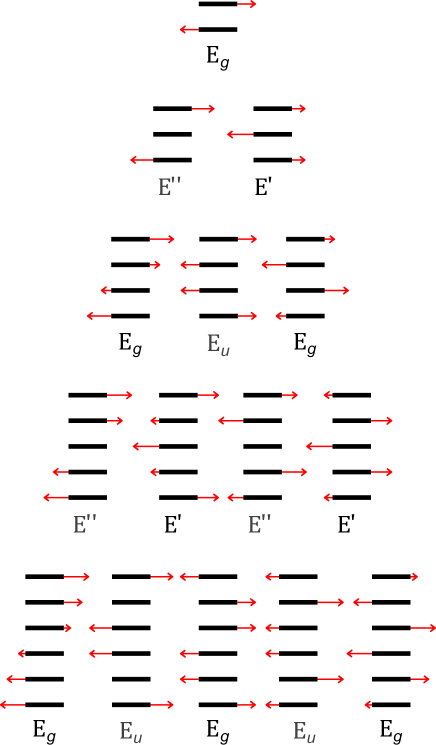
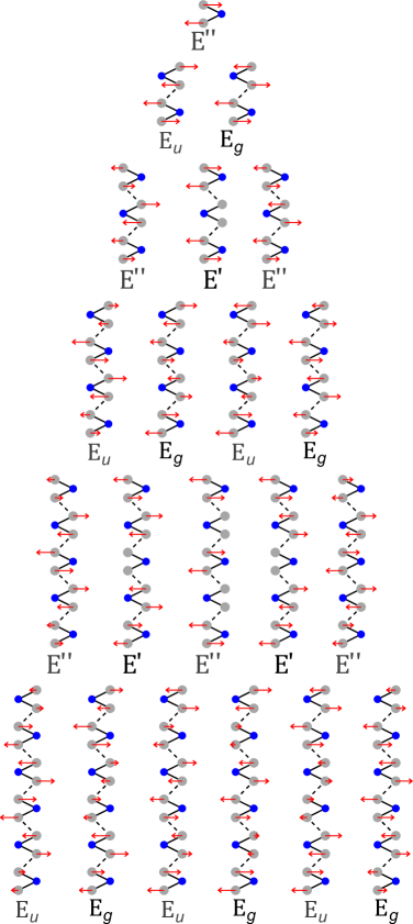
Figures S2 to S7 show the normal mode displacements associated with the LSM, iX, iMX, LBM, oX, and oMX modes in -layer MoTe2.
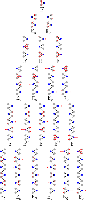
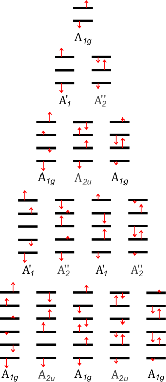
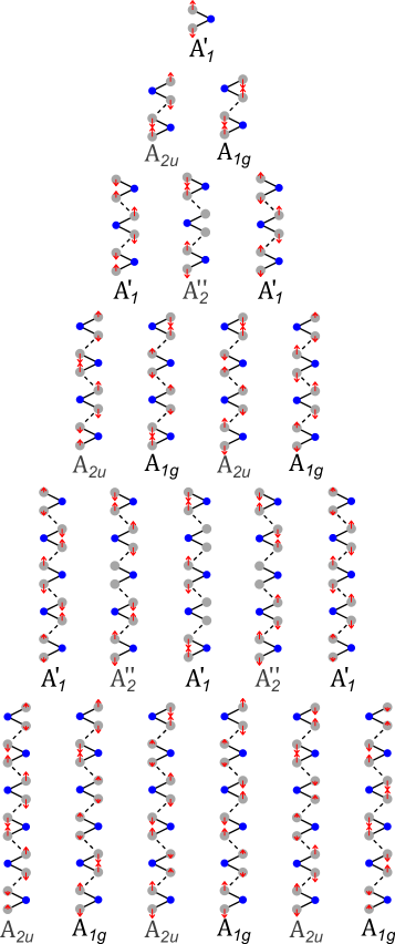
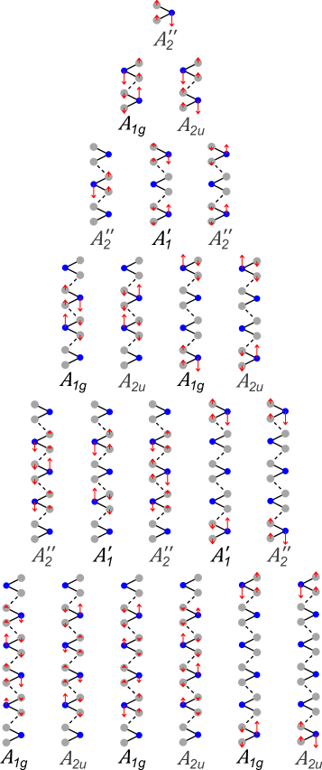
S4 The empirical bond polarizability model
In the Placzek approximation, the Raman intensity for non resonant first order scattering is given by
| (S15) |
where and are the polarizations of the incident and the scattered light respectively, is the Raman frequency, and with being the temperature. The Raman tensor is related to the change of the polarizability under atomic displacement. It can be calculated as
| (S16) |
where is the Cartesian component of atom of the orthonormal vibrational eigenvector is the atomic mass, and
| (S17) |
is the total energy in the unit cell, is a uniform electric field, is the component of the atomic displacement of the atom and is the electronic polarizability tensor.
The bond polarizability model approximates the total
polarizability of the atom as the sum of the individual
bond polarizabilities. Under the assumption that the bonds have cylindrical
symmetry, the polarizability tensor for a single bond can be written as
| (S18) | ||||
where and are longitudinal and perpendicular polarizabilities of the bond and are the components of the unit vector along the bond. Moreover, in the model, the polarizabilities depend only on the length of the bond (). The bond vector joining atoms to atom is given by
| (S19) |
and
| (S20) | ||||
Hence,
| (S21) |
where -. The contribution of a particular bond to the tensor is therefore
| (S22) |
with
| (S23) |
In the structure of MoTe2, the Molybdenum atom is bonded to six Tellurium atoms and the Tellurium atom is bonded to three Molybdenum atoms. In our calculations, we neglect the weak inter-layer bonds. That is the reason why we don’t get a finite peak for the (shear) mode with this model.
The calculated tensors are as follows:
The values of the constants , , and , in terms of the polarizabilities and their derivatives, obtained after substituting the MoTe2 lattice parameters are:
| (S24) | ||||
S5 Raman spectra from the bond polarizability model
With the bond polarizability model, we can assign a Raman intensity to each Raman frequency obtained with the
force constant model. While active Raman modes agree with group theory and experimental data, the model does not include Raman resonance effects, and some discrepancies arise when we compare with experimental spectra. Figure S8 shows the theoretical Raman spectra for the modes iX, oX, iMX, and oMX. The spectra for different values are offset for clarity. The iX mode has active subfeatures in layer MoTe2 and is in nice
agreement with the spectra of Fig. 3.
For the iMX mode, there are two close peaks for ; one being an inner mode (with lower frequency) and the other being a surface mode (with higher frequency). The difference in their frequencies is around 0.5 cm-1.The absolute intensity of the inner mode increases almost linearly with number of layers, as there are more layers vibrating, whereas the absolute intensity of the surface mode is independent of number of layers, as only the outer molecules are vibrating. As a result, the relative intensity of the surface mode drops as increases, and thus the maximum of the combined peak shifts to smaller
frequencies as increases.
In the case of the oX mode our model reproduces the active subfeatures well, but it fails in
describing the observed relative intensity between peaks. The highest frequency peak in the oX-mode feature has much larger relative intensity than the rest of the peaks in the model, which is in contrast to our measurements, where all the phonons
have comparable intensities. We can understand this result from the shape of the
tensors shown above. The largest contribution occurs when all the Te layers are out-of-phase with the neighboring Te layers. In case two layers vibrate
in-phase, they cancel each other, and therefore increasing the number of layers in-phase reduces
the intensity drastically. The similar intensity of the peaks suggest the participation of Raman resonance effects.
For the oMX mode, the surface phonons, which are split from the inner modes, have much larger intensity than the inner modes in the model. From the Raman tensors, if tellurium atoms in the same layer vibrate in-phase and with
identical amplitude, the intensity is identically zero. Only differences in the amplitudes can generate Raman
signal, which will be very small in comparison with the intensity of the oX modes. The largest amplitude differences
are due to surface phonons, which carry most of the contribution to the Raman intensity and it results in the
sole peak observed in the Raman spectra. A feature assigned to the inner modes is slightly visible in the measured spectra at eV (see Fig. 3(c) in the main text) but not at eV, which, again, suggests a resonance effect at eV, similar to the oX mode.
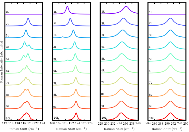
S6 Ab-initio bulk phonon modes
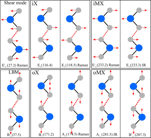
We have complemented the empirical model with ab-initio calculations of the phonon modes for bulk MoTe2. We have used density functional perturbation theory (DFPT) Baroni et al. (2001) as implemented in the Quantum Espresso code Giannozzi et al. (2009). We used the local-density approximation (LDA) which does not properly take into account van der Waals interaction between the layers but nevertheless gives decent result for the phonons of many layered systems because it overestimates the weak covalent part of the inter-layer bonding. The energy cutoff is 80 Ry, and the Monkhorst-Pack sampling of the grid is . The optimized lattice vectors are Åand Å. Figure S9 shows the ab-initio frequencies together with the corresponging phonon eigenvectors. We have grouped the phonon modes in Davydov pairs, except the shear and layer-breathing modes (whose “Davydov partner” would be a zero frequency acoustic mode). We observe a positive Davydov splitting for the iX, oX and oMX modes and a negative Davydov splitting for the mode iMX mode, as reported for other transition metal dichalcogenides Wieting et al. (1980). The calculated Davydov-splitting of the iX mode is 2.1 cm-1 (compared to the 2.7 cm-1 extrapolated from the measurements). For the oX mode, we obtain a splitting of 3.2 cm-1 (compared to 4.7 cm-1 from the experiments). The agreement between calculations and experiment is not perfect because of the lack of a proper treatment of van der Waals interaction with local exchange-correlation functionals. The predicted Davydov-Splitting for the oMX mode is 5.8 cm-1. For the calculation of the frequency of the mode, we have not taken into account the coupling to an external-electric field (Lydanne-Sachs-Teller interaction) that would lead to an up-shift of this mode. However, in layers of finite width, this interaction is absent.
S7 Additional Raman measurements
Figure S10 shows the raw Raman spectra of -layer MoTe2 recorded at and . Note that the iX mode has not been studied at due to the relatively large bandwidth of our Notch filter at .
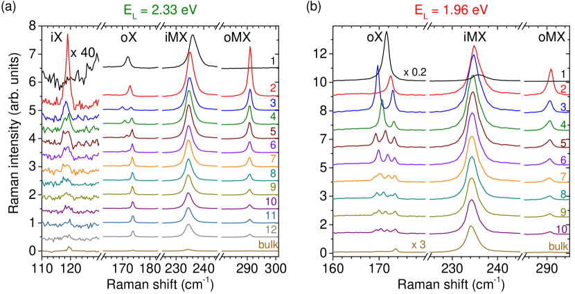
Figure S11 shows Raman spectra of the oX, iMX and oMX modes in -layer MoTe2 recorded at . The results recorded at are discussed in the main manuscript. At , the Davydov splitting also appears clearly for the oX feature, although the highest energy subfeature contains most of the oscillator strength for . The iMX feature also downshifts as increases and no appreciable splitting can be resolved. However, in contrast with our results at , the oMX feature does not exhibit any measurable splitting at .
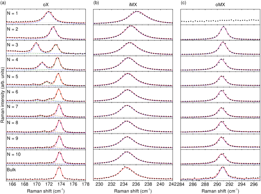
The corresponding fan diagrams associated with oX-, iMX and oMX-mode frequencies recorded at are shown in Fig. S12, together with the fan diagrams for oX and oMX modes extracted from the data recorded at and discussed in details in the main text. These two sets of data are very consistent with each other. Still, we can notice a small rigid shift of approximately which is smaller than the resolution of our experimental setup. This shift presumably arises from uncertainties (below our spectral resolution) in the calibration of our spectrometer. Importantly such a small shift has a negligible influence on the determination of the force constants. Indeed, the latter vary by less if one uses the oX, oMX and iMX frequencies recorded at instead of their values recorded at in the global fitting procedure described in the main manuscript.