High order eigenvalues for the Helmholtz equation in complicated non-tensor domains through Richardson Extrapolation of second order finite differences

Abstract

We apply second order finite difference to calculate the lowest eigenvalues of the Helmholtz equation, for complicated non-tensor domains in the plane, using different grids which sample exactly the border of the domain. We show that the results obtained applying Richardson and Padé-Richardson extrapolation to a set of finite difference eigenvalues corresponding to different grids allows to obtain extremely precise values. When possible we have assessed the precision of our extrapolations comparing them with the highly precise results obtained using the method of particular solutions. Our empirical findings suggest an asymptotic nature of the FD series. In all the cases studied, we are able to report numerical results which are more precise than those available in the literature.

1 Introduction

Among the different methods for estimating the eigenvalues and eigenfunctions of the Laplacian on a finite region of the plane, finite differences (FD) is the simplest, although the accuracy of the results obtained with this method is limited. In particular, for domains with reentrant corners with an angle of $\pi/\alpha$, it is well known that the error of the FD eigenvalues is dominated by a behavior $h^{2\alpha}$ for $h\rightarrow 0$ ($h$ is the grid spacing).

The so-called L-shaped membrane [$\alpha=4/3$] is a famous example which was studied long time ago by Fox, Henrici and Moler [14]. Because of the quite slow convergence of FD in this case ($\Delta E\approx h^{4/3}$), those authors applied an alternative method, the method of particular solutions (MPS), and, exploiting all the symmetries of the problem, they were able to obtain the first 8 digits of the lowest eigenvalue of the L-shape correctly, $E_{1}\approx 9.6397238$. Interestingly, the paper also mentions a precise (unpublished) value obtained by Moler and Forsythe, $E_{1}\approx 9.639724$, extrapolating the FD values obtained with very fine grids. Unfortunately, the extrapolation is neither named nor explained.

A valuable discussion of the Richardson extrapolation of FD results for the eigenvalues of the Laplacian on two dimensional regions of the plane is contained in [21], where it is pointed out that the correct exponents of the asymptotic behavior of $E_{1}$ for $h\rightarrow 0$ must be used in the extrapolation.

The purpose of the present paper is to show that is it possible to obtain quite precise approximations to the eigenvalues of the Laplacian on a certain class of two dimensional domains (specifically domains whose borders are sampled by the grid) by Richardson extrapolation of the FD results, provided that the asymptotic behavior of the FD eigenvalues for $h\rightarrow 0$ is taken into account correctly.

The paper is organized as follows: in section 2 we provide a general discussion of Richardson extrapolation, and its relation to the “method of deferred corrections”; in section 3, we describe the practical implementation of the Richardson extrapolation used in this paper; in section 4 we present the numerical results obtained for different domains, comparing them with the best results available in the literature; finally, in section 5 we summarize our findings and discuss possible directions of future work.

2 Richardson Extrapolation

Richardson Extrapolation is interpolation of samples of a sequence $S_{n}$ by a continuous function of a continuous variable $z$ followed by extrapolation to $z=0$ to approximate the limit of the sequence. The slowly convergent series $\sum_{n=1}^{\infty}n^{-2}$, for example, can be summed by taking the sequence of partial sums, $S_{\nu}=\sum_{n=1}^{\nu}n^{-2}$, to be samples of a function in $z\equiv 1/\nu$. In our application, the sequence is that of approximations to an eigenvalue by finite difference calculations whose asymptotic error is a series in some power of the grid spacing $h$; here $z=h^{2}$ [usually] or $z=h^{4/3}$ [for one singular application.]

The history including many independent discoveries is reviewed by Brezinski [7], Marchuk and Shaidurov [24], Sidi [33], Walz [37] and Joyce [20]. Christian Huyghens applied Richardson Extrapolation to estimate $\pi$ to 35 decimals from the perimeters of a sequence of polygons with more and more sides inscribed in the unit circle. Richardson’s (1927) paper [29] contained a plethora of examples that was the first comprehensive display of the power of extrapolation; he claimed no novelty but credited others including an obscure Russian language paper by Bogolouboff and N. Krylov Richardson Extrapolation of eigenvalues is discussed in Pryce’s book on numerical solution of Sturm-Liouville problems [27].

Richardson Extrapolation has four steps. First, compute samples $\{f(h_{n})\}$ of the function being extrapolated. Second, choose a set of basis functions $\{\phi_{j}(x)\}$ –– usually polynomials –– for an approximation

$$f_{N}(h)\equiv\sum_{j=1}^{N}\ a_{j}\,\phi_{j}(h)$$ (1)

The coefficients $a_{j}$ can always be computed by solving a matrix problem at a cost of $O(N^{3})$ operations, and this is necessary when the $\phi_{j}$ are a mixture of polynomials and polynomials multiplied by powers of $\log(x)$, for example. However, it is faster to use Neville-Aitken interpolation to compute a two-dimensional array (”Richardson Table”) of approximations of different $N$ formed from different subsets of the full sample set $\{f(h_{n})\}$. This is cheaper than matrix-solving [$O(N^{2})$ floating point operations] though this is only a small virtue because of the speed of modern laptops. More important, extrapolation is credible only if its answers are independent of numerical choices such as $N$ and subsets of the full set of samples. More precisely, a numerical answer is believable if and only if several different values of the numerical parameters yield the same answer to within the user chosen tolerance. The Richardson Table allows a quick search for such stable approximations. We shall return to this in analyzing each numerical example.

Various conventions are employed. A popular one is to arrange the table as a lower triangular matrix with $N$ samples of $f(z)$, the function being approximated, as the first column:

$$R_{j,1}=f(z_{j})$$ (2)

The simple recursion is

$$R_{j,k}=\frac{(z-z_{j-k-1})R_{j,k-1}-(z-z_{j})R_{j-1,k-1}}{z_{j}-z_{j-k+1}},\qquad k=j,(j+1),\ldots N,\,\,j=1,2,\ldots N$$ (3)

Each entry in column $k$ is a polynomial of degree $(k-1)$ which interpolates a subset of $k$ samples. The basic step combines two polynomials that interpolate $(k-1)$ points each to generate a polynomial that interpolates at the $k$ points $\{z_{j-k+1},\ldots z_{j}\}$. Both generators interpolate at the $(k-2)$ points $\{z_{j-k+1},\ldots z_{j}\}$, but only $R_{j,k-1}$ interpolates at $z_{j}$ while $R_{j-1,k-1}$ does not, but interpolates at $z_{j-k+1}$. It is easy to verify that

$$R_{j,k}(z=z_{j-k+1}) = \frac{(z_{j-k+1}-z_{j-k-1})R_{j,k-1}-(z_{j-k+1}-z_{j})R_{j-1,k-1}}{z_{j}-z_{j-k+1}}$$ (4)

$$= \frac{-(z_{j}-z_{j})}{z_{j}-z_{j-k+1}}R_{j-1,k-1}$$ (5)

$$= f(z_{j-k+1})\qquad[\mbox{using}\,R_{j-1,k-1}(z=z_{j-k+1})=f(z_{j-k+1})]$$ (6)

$$R_{j,k}(z=z_{j}) = \frac{(z_{j}-z_{j-k-1})R_{j,k-1}-(z_{j}-z_{j})R_{j-1,k-1}}{z_{j}-z_{j-k+1}}$$ (7)

$$= \frac{(z_{j}-z_{j-k-1}}{z_{j}-z_{j-k+1}}R_{j,k-1}$$ (8)

$$= f(z_{j}\qquad[\mbox{using}\,R_{j,k-1}(z=z_{j})=f(z_{j})]$$ (9)

$$R_{j,k}(z=z_{j-k+1}) = \frac{(z_{j-k+1}-z_{j-k-1})R_{j,k-1}-(z_{j-k+1}-z_{j})R_{j-1,k-1}}{z_{j}-z_{j-k+1}}$$ (10)

$$= \frac{-(z_{j}-z_{j})}{z_{j}-z_{j-k+1}}R_{j-1,k-1}$$ (11)

$$= f(z_{j-k+1})$$ (12)

$$R_{j,k}(z=z_{m}) = \frac{(z_{m}-z_{j-k-1})R_{j,k-1}-(z_{m}-z_{j})R_{j-1,k-1}}{z_{j}-z_{j-k+1}},\qquad m=j-k+2,\ldots{j-1}$$ (13)

$$= \frac{(z_{m}-z_{j-k-1})-(z_{m}-z_{j})}{z_{j}-z_{j-k+1}}f(z_{m})$$

$$= \frac{-z_{j-k-1}-z_{j})}{z_{j}-z_{j-k+1}}f(z_{m})$$ (14)

$$= f(z_{m})$$ (15)

where we used $R_{j,k-1}(z_{m})=R_{j-1,k-1}(z_{m})=f(z_{m})$ in the last lines.

For Richardson Extrapolation, we set $z=0$ and the table of polynomials becomes a lower triangular matrix of numbers.

When $z=1/n$, a reciprocal integer, Salzer gave a nice closed-form extrapolation formula in 1954 [30] as well as tables of the weights assigned to each sample in the final answer.

Sidi gives some convergence proofs in Chapter 3 of his book [33]. It is known that Richardson Extrapolation is often exponentially (geometrically) convergent with the error of the diagonals and bottom rows of the table falling as $\exp(-qn)$ for some positive constant $q$ even when the power series being extrapolated is factorially divergent, as usually true when the samples are of the trapezoidal rule for different grid spacings $h$ and the associated series in powers of $z=h^{2}$ is the Euler-Maclaurin formula. A comprehensive theory is still lacking, however.

Richardson Extrapolation is closely related to the “method of deferred corrections”, alternatively labelled “correction by higher order differences” in the (1983) book by Marchuk and Shaidurov [24]. “Deferred corrections” also solves matrix problems that are the low order, usually second-order, discretization of the problem. Deferred corrections also promotes this low order approximation into a very high order approximation. In contrast to Richardson Extrapolation, which solves the low order problem repeatedly on a variety of different grids, deferred corrections uses only a single grid, and applies an iteration preconditioned by the low order discretization [13, 5]. The residual is evaluated by a high order method; the accuracy of the converged iterative solution is equally high. One grid, instead of many, is obviously a significant advantage for deferred correction. The method can be applied to eigenvalue problems [36, 9].This approach has become the standard way of generating very high order time marching schemes to pair with spectral spatial discretizations. Dutt, Greengard and Rokhlin write, “We begin by converting the original ODE into the corresponding Picard equation and apply a deferred correction procedure in the integral formulation, driven by either the explicit or the implicit Euler marching scheme. The approach results in algorithms of essentially arbitrary order accuracy for both non-stiff and stiff problems” [12]. Further developments of Picard integral/deferred correction time-marching can be found in [18, 22, 19].

High order evaluation on a line in one dimension (time) is easy, but evaluating the residual of a partial differential equation by, say, twelfth order finite differences, is a bookkeeping nightmare. The programming and debugging escalate rapidly when the domain is geometrically complicated. Furthermore, corner singularities may make higher order evaluation of the residual impossible without heroic measures [6]. For all the success of deferred correction in other applications, for eigenproblems in domains with corners Richardson Extrapolation is clearly the better way.

3 Implementation of Richardson extrapolation

Suppose that we have calculated a given eigenvalue of the Laplacian on a certain domain using finite differences for a number of grids, which all sample the border, and with decreasing grid spacings, $h_{1}>h_{2}>\dots>h_{N}$. Only when $h\rightarrow 0$ is the exact eigenvalue of the associated problem in the continuum obtained, although the eigenvalues obtained for different (finite) grid spacing an asymptotic behavior, which depends on $h$; for the $k^{th}$ grid we may typically expect

$$E_{1}^{(k)}=c_{0}+\sum_{j=1}^{\infty}c_{j}h_{k}^{\alpha_{j}}$$ (16)

where $\alpha_{1}<\alpha_{2}<\dots<\alpha_{N}$. However, logarithms and more exotic functions have arisen in other problems. The exact values of these coefficients will depend on the particular properties of the domain studied: in fact, while integer values of $\alpha$ are associated with the discretization of the problem ($\alpha=2,4,\dots$), rational values of $\alpha$ may also appear when reentrant corners are present (as for the case of the L-shape where $\alpha_{1}=4/3$).

Using eq. (16) for all grids, and with basis functions $\phi_{j}$, one obtains a system of linear equations

$$\left\{\begin{array}[]{l}E_{1}^{(1)}=c_{0}\phi_{0}+c_{1}\phi_{1}(h_{1})+c_{2}\phi_{2}(h_{1})+\dots+c_{N-1}\phi_{N-1}(h_{1})+\dots\\ E_{1}^{(2)}=c_{0}\phi_{0}+c_{1}\phi_{1}(h_{2})c_{2}\phi_{2}(h_{2})+\dots+c_{N-1}\phi_{N-1}(h_{2})+\dots\\ \dots\\ E_{1}^{(N)}=c_{0}\phi_{0}+c_{1}\phi_{1}(h_{N})+c_{2}\phi_{2}(h_{N})+\dots+c_{N-1}\phi_{N-1}(h_{N})+\dots\\ \end{array}\right.$$ (21)

where the unknowns are the coefficients $c_{j}$ ($j=0,1,\dots,N-1$).

In matrix form these equations take the form

$$\mathbf{R}\left(\begin{array}[]{c}c_{0}\\ c_{1}\\ \dots\\ c_{N-1}\\ \end{array}\right)=\left(\begin{array}[]{c}E_{1}^{(1)}\\ E_{1}^{(2)}\\ \dots\\ E_{1}^{(N-1)}\\ \end{array}\right)$$ (30)

where

$$\mathbf{R}\equiv\left(\begin{array}[]{ccccc}\phi_{0}&\phi_{1}(h_{1})&\phi_{2}(h_{1})&\dots&\phi_{N-1}(h_{1})\\ \phi_{0}&\phi_{1}(h_{2})&\phi_{2}(h_{2})&\dots&\phi_{N-1}(h_{2})\\ \dots&\dots&\dots&\dots&\dots\\ \phi_{0}&\phi_{1}(h_{N})&\phi_{2}(h_{N})&\dots&\phi_{N-1}(h_{N})\\ \end{array}\right)$$ (35)

The solution to Eqs. (30) is obtained as

$$\left(\begin{array}[]{c}c_{0}\\ c_{1}\\ \dots\\ c_{N-1}\\ \end{array}\right)=\mathbf{R}^{-1}\left(\begin{array}[]{c}E_{1}^{(1)}\\ E_{1}^{(2)}\\ \dots\\ E_{1}^{(N-1)}\\ \end{array}\right)$$ (44)

where the extrapolated value of $c_{0}$ will provide an estimate of the exact eigenvalue.

Cramer’s rule can be used to obtain the coefficients $c_{j}$ without inverting the matrix $\mathbf{R}$; in particular

$$c_{0} = \frac{\left|\begin{array}[]{cccc}E_{1}&\phi_{1}(h_{1})&\dots&\phi_{N-1}(h_{1})\\ E_{2}&\phi_{1}(h_{2})&\dots&\phi_{N-1}(h_{2})\\ &\dots&&\\ E_{N}&\phi_{1}(h_{N})&\dots&\phi_{N-1}(h_{N})\\ \end{array}\right|}{\left|\begin{array}[]{cccc}\phi_{0}&\phi_{1}(h_{1})&\dots&\phi_{N-1}(h_{1})\\ \phi_{0}&\phi_{1}(h_{2})&\dots&\phi_{N-1}(h_{2})\\ &\dots&&\\ \phi_{0}&\phi_{1}(h_{N})&\dots&\phi_{N-1}(h_{N})\\ \end{array}\right|}$$ (53)

In our numerical examples

$$\phi_{j}(z)=z^{\alpha_{j}}$$ (54)

where $\alpha_{0}=1$ and the $\alpha_{j}$ are a monotonically increasing sequence of positive constants.

When we apply eq. (16) to the different grids, we are implicitly assuming that $\bar{h}>h_{1}>\dots>h_{N}$, where $\bar{h}$ is the radius of convergence of the series. However, in general $\bar{h}$ is unknown and it will only be estimated once the first few coefficients $c_{j}$ have been approximated. For this reason inaccurate results could be obtained if the spacing of one of the grids falls outside the radius of convergence of the asymptotic series. This is a common problem also of perturbative series, which are known to be divergent in many cases.

To avoid this problem, we can extrapolate by Padé rational approximation

$$E^{(k)}=\frac{c_{0}+\sum_{j=1}^{N}c_{j}h_{k}^{\alpha_{j}}}{1+\sum_{j=1}^{M}d_{j}h_{k}^{\beta_{j}}}$$ (55)

For integer exponents, $\alpha_{j}$ and $\beta_{j}$, and $N=M$, the choice $\alpha_{N}=\beta_{N}$, would correspond to a diagonal Padé. In a general case, with $N\neq M$ and rational exponents, we assume $\alpha_{N}=\beta_{M}$.

Using the different grids (in this case we use $N+M+1$ grids) we obtain the system of linear equations

$$E^{(1)} = c_{0}+c_{1}h_{1}^{\alpha_{1}}+\dots+c_{N}h_{1}^{\alpha_{N}}-d_{1}h_{1}^{\beta_{1}}E^{(1)}-\dots-d_{M}h_{1}^{\beta_{M}}E^{(1)}$$

$$E^{(2)} = c_{0}+c_{1}h_{2}^{\alpha_{1}}+\dots+c_{N}h_{2}^{\alpha_{N}}-d_{1}h_{2}^{\beta_{1}}E^{(2)}-\dots-d_{M}h_{2}^{\beta_{M}}E^{(2)}$$

$$\dots = \dots$$

$$E^{(N+M+1)} = c_{0}+c_{1}h_{N+M+1}^{\alpha_{1}}+\dots+c_{N}h_{N+M+1}^{\alpha_{N}}-d_{1}h_{N+M+1}^{\beta_{1}}E^{(N+M+1)}$$

$$- \dots-d_{M}h_{N+M+1}^{\beta_{M}}E^{(N+M+1)}$$

which can be cast in matrix form as

$$\tilde{\mathbf{R}}\left(\begin{array}[]{c}c_{0}\\ c_{1}\\ \dots\\ c_{N}\\ d_{1}\\ \dots\\ d_{M}\\ \end{array}\right)=\left(\begin{array}[]{c}E_{1}^{(1)}\\ E_{1}^{(2)}\\ \dots\\ E_{1}^{(M+N+1)}\\ \end{array}\right)$$ (67)

where

$$\tilde{\mathbf{R}}\equiv\left(\begin{array}[]{cccccccc}1&h_{1}^{\alpha_{1}}&\dots&h_{1}^{\alpha_{N}}&-h_{1}^{\beta_{1}}E^{(1)}&\dots&-h_{1}^{\beta_{M}}E^{(1)}\\ 1&h_{1}^{\alpha_{1}}&\dots&h_{2}^{\alpha_{N}}&-h_{2}^{\beta_{1}}E^{(2)}&\dots&-h_{2}^{\beta_{M}}E^{(2)}\\ \dots&\dots&\dots&\dots&\dots&\dots&\dots\\ 1&h_{N+M+1}^{\alpha_{1}}&\dots&h_{N+M+1}^{\alpha_{N}}&-h_{N+M+1}^{\beta_{1}}E^{(N+M+1)}&\dots&-h_{N+M+1}^{\beta_{M}}E^{(N+M+1)}\\ \end{array}\right)$$ (72)

The solutions to these equations are found inverting $\tilde{R}$

$$\left(\begin{array}[]{c}c_{0}\\ c_{1}\\ \dots\\ c_{N}\\ d_{1}\\ \dots\\ d_{M}\\ \end{array}\right) = \tilde{\mathbf{R}}^{-1}\left(\begin{array}[]{c}E_{1}^{(1)}\\ E_{1}^{(2)}\\ \dots\\ E_{1}^{(M+N+1)}\\ \end{array}\right)$$ (84)

or using Cramer’s rule once again.

4 Numerical results

To apply the extrapolation schemes described in the previous section we need to calculate accurately the FD eigenvalues for a series of grids. We consider different domains, with borders which can be sampled by a square grid and with different reentrant angles.

4.1 L-shaped domain

We consider the L-shaped region $\Omega\equiv\left\{|x|<1,|y|<1\right\}-\left\{0\leq x<1,0\leq y<1\right\}$, represented in Fig. 1. Using finite differences and a five-points approximation to the Laplacian, the Helmholtz equation on $\Omega$ is solved with Dirichlet boundary conditions on $\partial\Omega$ for a series of grids with an increasing number of points. We have exploited the symmetry of the domain, to obtain separately the even and odd modes of the L-shape.

Our numerical calculations consist of two sets:

• A calculation of the lowest eigenvalue of the L, using $124$ grids with spacing $h=1/N_{0}$ and $N_{0}=10,\dots,133$. The finite difference results of this set are obtained using the ”Conjugate Gradient Method” (CGM), as described in Ref. [26], and they are accurate to $220$ digits;

• A calculation of the lowest $100$ eigenvalues of the L, using 100 grids with spacing $h=1/N_{0}$ and $N_{0}=10,\dots,109$. The finite difference results of this set are obtained using the internal Mathematica command

  igenvalues   and
  they are accurate to $60$ digits.
  \end{itemize}
  In Table \ref{tab_results_L} we report the available estimates of the lowest eigenvalue of the L-shape in the literature,
  including the results of the present work.
  \begin{table}[t]
  \caption{Available estimates of the lowest eigenvalue of the L-shape (smaller fonts are used for the last three values, to allow fitting
  the results in the column).}
  \bigskip
  \label{tab_results_L}
  \begin{center}
  \begin{tabular}{|l|l|}
  \hline
   & $

  _1$\\ {\hline}ReidandWalsh\cite[cite]{[\@@bibref{}{Reid65}{}{}]}9.63972\\ Fox,HenriciandMoler\cite[cite]{[\@@bibref{}{Fox67}{}{}]}9.6397238\\ Mason\cite[cite]{[\@@bibref{}{Mason67}{}{}]}9.6397\\ Sideridis\cite[cite]{[\@@bibref{}{Sideridis84}{}{}]}9.6395\\ Schiff\cite[cite]{[\@@bibref{}{Schiff88}{}{}]}9.659\\ ChristiansenandPetersen\cite[cite]{[\@@bibref{}{ChristiansenPetersen89}{}{}]}9.6397238{\tiny 3991}\\ Still\cite[cite]{[\@@bibref{}{Still03}{}{}]}$9639723^{96}_{71}$\\ BetckeandTrefethen\cite[cite]{[\@@bibref{}{Betcke05}{}{}]}9.6397238440219\\ Amore\cite[cite]{[\@@bibref{}{Amore08}{}{}]}9.6397238440\\ YuanandHe\cite[cite]{[\@@bibref{}{He09}{}{}]}$9.63972384^{44}_{04}$\\ thiswork{\bf\tiny(Richardson)}{\tiny 9.63972384402194105271145926236482315626728952582190645}\\ thiswork{\bf\tiny(Pad\'{e}-Richardson)}{\tiny 9.6397238440219410527114592623648231562672895258219064561095797005640}\\ thiswork{\bf\tiny(MPS)}{\tiny 9.639723844021941052711459262364823156267289525821906456109579700564036}\\ {\hline}$

  
  

As we have mentioned before, the convergence of the numerical results is affected by the presence of a reentrant corner and the finite-difference eigenvalue $E(h)$ behaves for $h\rightarrow 0$ as[10, 21]

$$E(h)=E(0)+ah^{4/3}+\dots$$ (85)

where $E(0)$ is the eigenvalue of the Laplacian in the continuum. For the related problem of a H-shaped membrane, Donnelly [10] conjectured the asymptotic behavior

$$E(h)=E(0)+ah^{4/3}+bh^{2}+ch^{10/3}+dh^{4}+\dots$$ (86)

for the fundamental eigenvalue . This behavior was also used by Christiansen and Petersen [8] to perform a Richardson extrapolation of the finite difference results for the L-shape (see Table LABEL:tab_results_L).

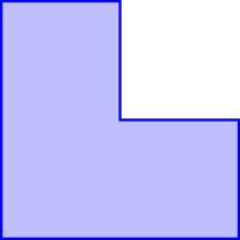
Figure 1: L-shaped region

The results obtained extrapolating the FD sequences can be compared with the precise results obtained with the ”method of multiple solutions” (MPS)[14]. Table 1 reports the first $25$ eigenvalues of the L-shape obtained with the MPS (for the case of the first eigenvalue we have used 545 points evenly spaced, which allow one to obtain 70 digits of precision, for the remaining cases we have used $425$ points, which allows an accuracy of about 50 digits). The eigenvalues marked with $\dagger$ are known exactly and correspond to modes of a square. The MPS has been implemented in Mathematica 10 [38], taking advantage of Mathematica’s ability to work with arbitrary precision numbers or with a large number of digits (in our case typically numbers are specified to 100 digits).

We will use these values to establish the accuracy of the approximate values of $E_{n}$ obtained by applying four different extrapolation schemes, differing in the choice of the exponents:

• Extrapolation ${\rm i}$

  $$E(h) = E(0)+\sum_{n=1}^{\infty}c^{(i)}_{n}h^{2n}\approx E(0)+c^{(i)}_{1}h^{2}+c^{(i)}_{2}h^{4}+O(h^{6})$$ (87)

• Extrapolation ${\rm ii}$

  $$E(h) = E(0)+\sum_{n=1}^{\infty}c^{(ii)}_{n}h^{n}\approx E(0)+c^{(ii)}_{1}h^{2}+c^{(ii)}_{2}h^{3}+O(h^{4})$$ (88)

• Extrapolation ${\rm iii}$ (Donnelly, Ref. [10])

  $$E(h) = E(0)+\sum_{n=1}^{\infty}\left[c^{(iii)}_{2n-1}h^{2n-2/3}+c^{(iii)}_{2n}h^{2n}\right]$$ (89)

  $$\approx E(0)+c^{(iii)}_{1}h^{4/3}+c^{(iii)}_{2}h^{2}+c^{(iii)}_{3}h^{10/3}+O(h^{4})$$

• Extrapolation ${\rm iv}$

  $$E(h) = E(0)+\sum_{n=1}^{\infty}c^{(iv)}_{n}h^{2(n+1)/3}$$ (90)

  $$\approx E(0)+c^{(iv)}_{1}h^{4/3}+c^{(iv)}_{2}h^{2}+c^{(iv)}_{3}h^{8/3}+O(h^{10/3})$$

The first two schemes only use integer exponents and are expected to be accurate only for the modes of the L-shape which are also modes of the square.

Figure 2 displays the error $|E_{1}^{(extra)}-E_{1}^{(MPS)}|$ for the lowest eigenvalue of the L-shaped region, using the third and fourth extrapolation schemes. Here

$$\Delta_{a} = |\mathcal{R}^{(k,124)}(E_{1})-E_{1}^{(MPS)}|$$ (91)

$$\Delta_{b} = |\mathcal{R}^{(k,124)}(E_{1})-\mathcal{R}^{(k-1,124)}(E_{1})|$$ (92)

where the superscripts $(iii)$ and $(iv)$ refer to the series used and the FD eigenvalues are accurate to 220 digits. The values $\Delta_{c}^{(iv)}$ are the analogous of $\Delta_{a}^{(iv)}$, but using FD eigenvalues are accurate to 60 digits.

The approximations obtained with the first two schemes, which do not use rational exponents, are very poor for this mode.

In particular, the extrapolated values in the four cases are

• Extrapolation ${\rm i}$

  $$E_{1}\approx\underline{9.639}8$$ (93)

• Extrapolation ${\rm ii}$

  $$E_{1}\approx\underline{9.6397}327$$ (94)

• Extrapolation ${\rm iiii}$

  $$E_{1}\approx\underline{9.639723844021}1929465$$ (95)

• Extrapolation ${\rm iv}$ (corresponding to the minimum in Fig. 2)

  $$E_{1}\approx\underline{9.639723844021941052711459262364823156267289525821906456}458$$ (96)

Remarkably, the fourth scheme provides the first $55$ digits of $E_{1}$ for the L-shape correctly, suggesting that the the exact asymptotic behavior of the finite difference eigenvalues, for $h\rightarrow 0$, is $E(h)=E(0)+\sum_{n=1}^{\infty}c^{(iv)}_{n}h^{2(n+1)/3}$.

In correspondence to the minimum of Fig. 2 we have calculated the first few coefficients of the asymptotic series for the eigenvalue of the fundamental mode; the expansion reads (underlined digits are expected to have converged)

$$E(h) \approx \underline{9.63972384402194105271145926236482315626728952582190645}6$$ (97)

$$+ \underline{2.19759909080385142157537952672409583683648557094}5\ h^{4/3}$$

$$- \underline{5.254349649878412271190008297029240841285038851}0\ h^{2}$$

$$- \underline{0.045716100985365949827658978449794728350032}8\ h^{8/3}$$

$$- \underline{1.946468144036811059220897747699440650587}7\ h^{10/3}$$

$$+ \underline{1.125074754927755172836371946813777186}1\ h^{4}$$

$$- \underline{0.2147544087374345021476728527871998}5\ h^{14/3}$$

$$+ \underline{0.35588422353456505262712958896229}4\ h^{16/3}$$

$$+ \underline{0.006403070910486707732478038349}7\ h^{6}$$

$$+ \underline{0.038286091425541761563564936}0\ h^{20/3}$$

$$- \underline{0.0730523282127573068239088}6\ h^{22/3}+\dots$$

The behavior of the error in Fig. 2 suggests that the FD series is asymptotic. Therefore, if one picks a set of grids with spacings $h_{1}>h_{2}>\dots$, it is convenient to perform an extrapolation using the grids up to a given spacing $h_{N}$ where the error reaches a minimum.

This behavior, however, does not limit the number of accurate digits of the eigenvalue that one can obtain using the Richardson extrapolation. This is illustrated in Figs. 3 and 4: the first figure is obtained extrapolating the FD results of a set with smallest spacing $h_{min}$ and determining the minimum error over the extrapolated eigenvalue (which will correspond to the minimum observed in Fig. 2). In this case we observe that the number of accurate digits of the extrapolated eigenvalue grows linearly for $N_{0}\gg 1$. Of course this behavior will be lost when the number of digits of the FD eigenvalue is not sufficient (see for example, the last curve of Fig. 2, where the FD eigenvalue are only accurate to 60 digits). Fig. 4 illustrates the fact that, as $h_{min}$ gets smaller and smaller, the number of grids used in the optimal extrapolation also grows linearly.

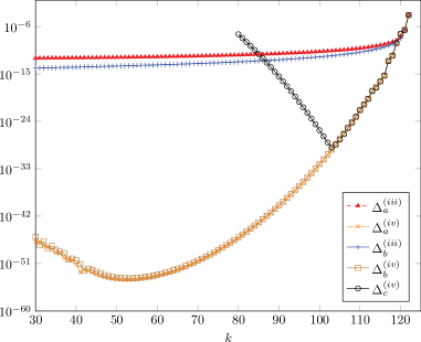
Figure 2: Error over the first eigenvalue of the L-shaped region. The first two curves report the difference between the values obtained with Richardson extrapolation of $124-k$ grids, respectively using scheme ${\rm iii}$ and ${\rm iv}$, and the precise value that we have obtained with the MPS; the last two curves report the difference between the values obtained with Richardson extrapolation of $124-k$ grids and the values obtained with Richardson extrapolation of $124-k-1$ grids, respectively using scheme ${\rm iii}$ and ${\rm iv}$. This difference essentially provides the number of stable digits achieved. In the first four curves the FD eigenvalues are obtained with an accuracy of 220 digits; the last curve is analogous to the second one, limiting the accuracy of the FD eigenvalues to 60 digits

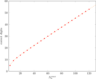
Figure 3: Correct digits of the lowest eigenvalue of the L-shaped membrane obtained with Richardson extrapolation using a set of FD grids with a smallest spacing $h_{min}=1/N_{0}^{max}$. Notice that the number of grids used for a given $h_{min}$ depends on $h_{min}$ itself (see Fig. 4). The dashed curve is the fit $f(n)=7.23166\,+0.383229n-\frac{20.9176}{n}$. The FD eigenvalues used in the extrapolation were computing using 220 decimal digit floating point arithmetic.

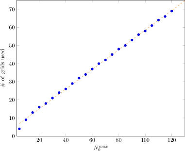
Figure 4: Optimal number of FD grids used for a set of FD grids with smallest spacing $h_{min}=1/N_{0}^{max}$. The dashed curve is the fit $g(n)=0.542696n+4.20652$. The FD eigenvalues used in the extrapolation were computed in multiple precision floating point arithmetic with a precision of 220 decimal digits.

In Fig. 5 we have applied the Padé-Richardson extrapolation to calculate the error over the fundamental eigenvalue of the L. Here $\mathcal{P}^{(k,124)}$ indicates the diagonal Padé with $2k+1$ coefficients, which uses the grids going from $124-2k$ to $124$. The horizontal line corresponds to the lowest error obtained with the Richardson extrapolation, i.e. to the minimum of Fig. 2. The errors are obtained using as a reference the precise estimate obtained using the MPS with 545 points distributed on the border, which is expected to have at least 70 correct digits (see Table LABEL:tab_results_L).

The result obtained with the Padé-Richardson extrapolation contains 13 extra digits of accuracy with respect to the result obtained with the Richardson extrapolation alone!!

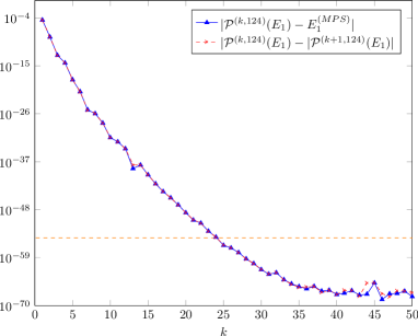
Figure 5: Error in the first eigenvalue of the L-shpaed domain using the diagonal Padé-Richardson Extrapolation $\mathcal{P}^{(k,124)}$. The horizontal line corresponds to the minimal error obtained with the Richardson extrapolation, corresponding to the minimum in Fig. 2.

The same analysis can be carried out for the eigenvalue of the first excited mode of the L-shaped membrane, which is odd with respect to reflection about the line $y=x$; also in this case, the fourth scheme is the appropriate one and the asymptotic expansion is obtained

$$E(h) \approx \underline{15.19725192645434327487838213300054590}06+3.18\cdot 10^{-32}\ h^{4/3}$$ (98)

$$- \underline{12.565568615260003775714180770}53\ h^{2}$$

$$- \underline{2.2529040988480935561491817}46\ h^{8/3}-9.9\cdot 10^{-25}\ h^{10/3}$$

$$+ \underline{3.932508901213713526500}07\ h^{4}+\underline{1.1289729308101123792}42\ h^{14/3}$$

$$+ \underline{0.950164117523872693}21\ h^{16/3}-\underline{1.36902891120799}30\ h^{6}$$

$$- \underline{0.0740361191169}66\ h^{20/3}+\underline{0.772459685647}50\ h^{22/3}+\dots$$

Notice that in this case we have used the less precise set of FD values, which were computed only in 60 digit floating point arithmetic: the eigenvalue of the first excited state is now reproduced with “just” 37 correct digits.

This result clearly shows that the coefficients of the terms $h^{4/3}$ and $h^{10/3}$ must vanish: in particular it is easy to understand the absence of $h^{4/3}$ since the mode that we are calculating is the fundamental eigenmode of the desymmetrized region obeying Dirichlet boundary conditions on $y=x$. In this case the reentrant corner is $\pi/\alpha=3\pi/4$ and therefore $2\alpha=8/3$.

With this simple observation, eliminating $4/3$ and $10/3$ from the exponents used in the extrapolation scheme, we are able to obtain 3 more digits of $E_{2}$

$$\log_{10}\frac{1}{|E_{2}^{({\rm RE})}-E_{2}^{\rm(MPS)}|}=40.8$$

Even more digits can be obtained using the Padé-Richardson scheme, without the exponents $4/3$ and $10/3$: in this case

$$\log_{10}\frac{1}{|E_{2}^{({\rm PRE})}-E_{2}^{\rm(MPS)}|}=45.8$$

Table 1: Lowest 25 eigenvalues of the L-shaped domain obtained with the MPS using $425$ points evenly spaced on the border. The eigenvalues marked with $\dagger$ are known exactly; the first eigenvalue, marked with $*$, has been obtained using the MPS with $545$ points.

$n$	$E_{n}^{({\rm MPS})}$
1∗	9.639723844021941052711459262364823156267289525821906456109579700564036
2	15.197251926454343274878382133000545900777179939609
3†	$2\pi^{2}$
4	29.521481114144883298220387998949268230835182037083
5	31.912635957137762200327505645485619891180683442197
6	41.474509890214922338810104064796906887679915692804
7	44.948487781351230152829670239630032397049780134665
8†	$5\pi^{2}$
9†	$5\pi^{2}$
10	56.709609887385120714216741638492259079610565870838
11	65.376535709845878509384400627738811907191161706097
12	71.057755648513529930798223378765313509589316160842
13	71.572679680336556014706999077329408038228565031443
14	$8\pi^{2}$
15	89.301668351960185629207557215836143584908527108716
16	92.306906763049247832266397297040944898714305036279
17	97.380722646021860253461536778106579066564981169123
18	$10\pi^{2}$
19	$10\pi^{2}$
20	101.60529408377871548543481415097538087072356189211
21	112.36860922562569413546584663077376004912074741174
22	115.52017309466770886932756039014897616475657545671
23	$13\pi^{2}$
24	$13\pi^{2}$
25	130.11902885096790256577606801292831058988583848246

Table 2: Correct digits of the first 25 eigenvalues of the L-shaped domain, obtained applying the Richardson and Richardson-Padé extrapolations to FD eigenvalues. The values marked with the $\dagger$ correspond to eigenstates of the square. The first eigenvalue has been obtained extrapolating the FD eigenvalues of $124$ grids, obtained with a floating point precision of 220 digits.

$n$	scheme	$\log_{10}\frac{1}{|E_{n}^{({\rm RE})}-E_{n}^{\rm(MPS)}|}$	$\log_{10}\frac{1}{|E_{n}^{({\rm PRE})}-E_{n}^{\rm(MPS)}|}$	parity
1∗	${\rm iv}$	54.5	67.5	${\rm even}$
2	${\rm iv}$	40.8	45.8	${\rm odd}$
3†	${\rm i}$	62.9	73.1	${\rm even}$
4	${\rm iv}$	37.1	45.8	${\rm odd}$
5	${\rm iv}$	35.9	42.6	${\rm even}$
6	${\rm iv}$	35.1	42.2	${\rm even}$
7	${\rm iv}$	36.7	44.5	${\rm odd}$
8†	${\rm i}$	60.6	73.9	${\rm odd}$
9†	${\rm i}$	60.8	73.8	${\rm even}$
10	${\rm iv}$	35.2	41.9	${\rm even}$
11	${\rm iv}$	34.5	42.6	${\rm odd}$
12	${\rm iv}$	34.8	42.2	${\rm even}$
13	${\rm iv}$	34.4	42.6	${\rm odd}$
14†	${\rm i}$	60.3	73.2	${\rm even}$
15	${\rm iv}$	33.4	41.3	${\rm even}$
16	${\rm iv}$	30.8	39.9	${\rm odd}$
17	${\rm iv}$	30.6	39.3	${\rm odd}$
18†	${\rm i}$	60.3	74.0	${\rm odd}$
19†	${\rm i}$	59.5	73.9	${\rm even}$
20	${\rm iv}$	33.0	40.7	${\rm even}$
21	${\rm iv}$	32.6	40.0	${\rm even}$
22	${\rm iv}$	33.7	42.6	${\rm odd}$
23†	${\rm i}$	59.6	73.6	${\rm odd}$
24†	${\rm i}$	59.7	73.2	${\rm even}$
25	${\rm iv}$	33.3	43.4	${\rm odd}$

4.2 H-shaped domain

We now consider a domain with the shape of H, displayed in Fig. 3, originally studied by Donnelly [10] using the method of particular solutions (MPS) and finite differences (FD). As we have already mentioned in the previous section, the author conjectured that the FD eigenvalues, corresponding to a given grid spacing $h$, behave as

$$E(h)=E(0)+ah^{4/3}+bh^{2}+ch^{10/3}+dh^{4}+\dots$$ (99)

where $E(0)$ is the corresponding eigenvalue of the Laplacian in the continuum and the exponent $4/3$ is determined by the presence of a reentrant corner $3\pi/2$ [10, 21].

As for the L-shape, we want to obtain a precise estimate of the lowest eigenvalues for this problem, using a sequence of FD eigenvalues, obtained for different grids. Notice that the eigenfunctions of the Laplacian on this domain can be classified according to four different symmetry classes, even-even, even-odd, odd-even and odd-odd with respect to reflection about the $x$ and $y$ axes. By working separately on the modes belonging to each class, the computational complexity of the problem can be reduced and finer grids can be studied. Our present analysis, in particular, is limited to the even-even modes. The spacing of the grid is chosen so that the border of the H-shaped is sampled exactly and it corresponds to $h_{k}=3/2/(9+3(k-1))$, with $k=1,2,\dots$. We have calculated the first $25$ eigenvalues of the even-even modes of the H-shape with a floating point precision of $60$ digits, for the grids corresponding to $k=1,2,\dots,40$.

Our results for the lowest eigenvalue should be compared with those of Donnelly [10]

$$E_{1}^{(Donnelly)}=7.7330889$$ (100)

and, more recently, of Betcke and Trefethen [3]

$$E_{1}^{(BT)}=7.7330888559$$ (101)

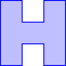
Figure 6: H-shaped region

In Fig. 7 we report the error over the first eigenvalue of the H-shape. The first two curves report the difference between the values obtained with Richardson extrapolation of $40-k$ grids, respectively using scheme ${\rm iii}$ and ${\rm iv}$, and the precise value of Betcke and Trefethen [3]. However, since the results of Ref. [3] are not sufficiently precise, it is convenient to estimate the error using the difference between the values obtained with Richardson extrapolation of $40-k$ grids and the values obtained with Richardson extrapolation of $40-k-1$ grids, respectively using scheme ${\rm iii}$ and ${\rm iv}$. This difference essentially provides the number of stable digits achieved. Notice that the second curve rapidly reaches a plateau, for $k\leq 34$, signaling that in this range the extrapolated results are more precise than those of Ref. [3].

The figure clearly shows that the asymptotic behavior conjectured by Donnelly in Ref. [10] is not correct; our best estimate of the fundamental eigenvalue corresponds to the last curve in Fig. 7 (i.e. scheme iv) for $k=18$:

$$E_{1}=7.7330888559426190667$$ (102)

where all the digits are believed to be correct.

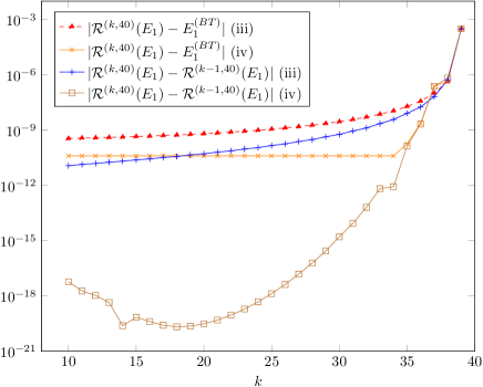
Figure 7: Error over the first eigenvalue of the H-shaped region. The first two curves report the difference between the values obtained with Richardson extrapolation of $40-k$ grids, respectively using scheme ${\rm iii}$ and ${\rm iv}$, and the precise value of Betcke and Trefethen [3]; the last two curves report the difference between the values obtained with Richardson extrapolation of $40-k$ grids and the values obtained with Richardson extrapolation of $40-k-1$ grids, respectively using scheme ${\rm iii}$ and ${\rm iv}$. This difference essentially provides the number of stable digits achieved.

In table  3 we report the approximate values of the first 24 eigenvalues of the even-even modes of the H-shape obtained using Richardson extrapolation. It is particularly interesting to consider the value for the mode 24, which has the lowest precision. The coefficients of the asymptotic series obtained from the Richardson extrapolation are (underlined digits are expected to have converged)

$$E(h) \approx \underline{194.7347257248}53+\underline{1.2880}50h^{4/3}-\underline{2861.993}46h^{2}$$ (103)

$$- \underline{25.7}61h^{8/3}+\underline{51}5.6h^{10/3}+\underline{14}691.3h^{4}+\dots$$

The coefficients of this series, although determined with less precision than in the cases discussed earlier for the L-shape, clearly suggest the presence of a smaller radius of convergence, which drastically affects the accuracy of the calculation.

Table 3: Lowest 24 eigenvalues of even-even modes of the H-shaped domain obtained using Richardson extrapolation with set ${\rm iv}$ (the sets marked with $\dagger$ are eigenstates of the square and are extrapolated using set ${\rm i}$).

$n$	$E_{n}^{({\rm Richardson})}$
1	7.7330888559426190667
2	14.30522996107150163018552
3†	19.73920880217871723766898199975230227062739
4	33.0048892952083545188
5	37.2054234400574157525
6	46.2961910861973723751
7	58.7501048292892847997
8	63.113298546574958190
9	67.43457224647486521
10	85.80372978847046992
11	92.12485042399187898
12	95.7615825533281487
13†	98.696044010893586188344909998
14	112.42755013401679304
15	122.557976404091254965
16	133.5364354179283
17	139.4282184592822
18	142.4312241050896
19	150.543062476658690
20	164.339040164448839
21	171.85972578742946
22†	177.652879219608455139020837997770
23	180.46602205029118
24	194.7347257248

4.3 Isospectral domains

Consider the domains of Fig. 8. It is known that these domains are isospectral, i.e. that the eigenvalues of the laplacian on one domain coincide with those on the second domain, as proved by Gordon, Webb and Wolpert [17, 16]. The numerical calculation of the eigenvalues of these regions has attracted large interest, using different techniques; for example, Wu, Sprung and Martorell [39] have used finite difference and mode matching to estimate the first 25 eigenvalues of these domains; the most precise results have been obtained by Driscoll in Ref. [11] and by Betcke and Trefethen [3]. The result that Betcke and Trefethen report for the eigenvalue of the fundamental mode

$$E_{1}\approx 2.537943999798$$

is slightly more precise than the value reported by Driscoll. Moreover, Sridhar and Kudrolli [34] have performed an experiment with microwave cavities of the form of the domains of Fig. 8, verifying their isospectrality .

In this case, we have applied finite differences calculating the lowest eigenvalues of both domains for 30 grids; the grid spacing is chosen appropriately so that the border is sampled exactly . Remarkably, the matrices obtained with finite difference for the two domains are also isospectral.

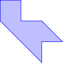
Figure 8: Isospectral domains

In Fig. 9 we report the error over the first eigenvalue of the isospectral domains, while in Table 4 we report our best estimates for the lowest 25 eigenvalues, obtained using Richardson extrapolation, with the same exponents as for the L. For the lowest eigenvalue we gain 5 digits with respect to the result of Betcke and Trefethen

$$E_{1}=2.53794399979862045$$ (104)

Moreover, even our poorest result, for the 25th mode, has two extra digits with respect to the result of Driscoll.

In light of these results, we stress that the finite difference method can provide very accurate results, despite the common prejudices. In the abstract of the paper of Driscoll, for example, we read: ”Furthermore, standard numerical methods for computing the eigenvalues, such as adaptive finite elements, are highly inefficient”.

A second comment regards the work of Wu, Sprung and Martorell, who calculated the FD eigenvalues for these domains for 3 grids and then used Richardson extrapolation to obtain better estimates. Incorrectly, they assumed that the FD results vary quadratically with the grid spacing, a behavior which is appropriate only for the modes of the square (modes 9 and 21).

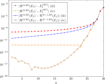
Figure 9: Error over the first eigenvalue of the isospectral regions. The first two curves report the difference between the values obtained with Richardson extrapolation of $30-k$ grids, respectively using scheme ${\rm iii}$ and ${\rm iv}$, and the precise value of Betcke and Trefethen [3] ($E_{1}\approx 2.537943999798$); the last two curves report the difference between the values obtained with Richardson extrapolation of $30-k$ grids and the values obtained with Richardson extrapolation of $30-k-1$ grids, respectively using scheme ${\rm iii}$ and ${\rm iv}$. This difference essentially provides the number of stable digits achieved.

Table 4: Lowest 25 eigenvalues of the isospectral domains obtained using Richardson extrapolation with set ${\rm iv}$ (the sets marked with $\dagger$ are eigenstates of the square and are extrapolated using set ${\rm i}$).

$n$	$E_{n}^{({\rm Richardson})}$
1	2.53794399979862045
2	3.65550971352441826
3	5.17555935622451540
4	6.53755744376443310
5	7.2480778625641275588
6	9.20929499840321242
7	10.59698569133316780
8	11.5413953955859566289
9†	12.33700550136169827354311374984518891914212
10	13.0536540557280658
11	14.313862464291008706
12	15.871302620009314
13†	16.941751687972089
14	17.6651184368431201
15	18.9810673876525993
16	20.882395043282328
17	21.2480051773728
18	22.23285179297328
19	23.711297484824032
20	24.479234069273887
21†	24.674011002723396547086227499690377838284
22	26.08024009965984
23	27.304018921125
24	28.175128581453
25	29.569772913239

4.4 Square domain with a $45^{0}$-crack

The domain represented in Fig. 10 is particularly interesting, since it contains a reentrant angle $\theta=7\pi/4$, which is larger than the angle of the L-shaped domain. Additionally, the domain has no symmetry and therefore the numerical calculation is more demanding than for the case of the L and H shapes. This problem has been originally studied by Blum and Rannacher [4] and more recently by Yuan and He [40], where the bounds

$$35.631515\leq E_{1}\leq 35.631522$$

have been obtained. The result $E_{1}\approx 35.617$ was obtained in Ref. [4] applying Richardson extrapolation to finite elements.

In Table 5 we report the numerical approximations to the lowest 5 eigenvalues of this domain, obtained using the MPS with 356 points. The digits reported in the table are expected to be correct; in particular for the lowest eigenvalue we have

$$E_{1}\approx 35.63151951719172309520548614207765698409$$ (105)

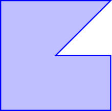
Figure 10: Unit square with a $45^{0}$-crack

In Fig. 11 we show a contour plot of the first four modes of this domain, obtained using finite differences with a grid with spacing $h=1/120$, corresponding to a total of 12331 grid points. The solid blue lines are the nodal lines, while the dashed green lines are level curves. While the fundamental mode is nodeless, the remaining three states have one or two nodal lines which start on the vertex of the reentrant corner, thus dividing the original domain in two or more domains. Looking at the figure we see that for the second state the resulting sub-domains have a reentrant angle $\theta=7\pi/8$, while for the third and fourth states the sub-domains have a reentrant angle $\theta=7\pi/12$. The dashed straight lines in the plot are tangent to the nodal line in the vertex.

As a result of this observation, we speculate that the asymptotic behavior of the finite difference eigenvalue may contain the exponents $8/7$, $16/7$ and $24/7$ .

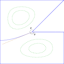
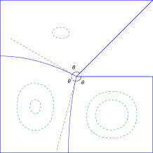
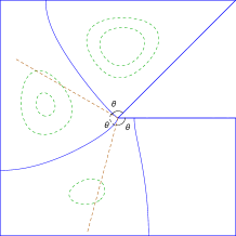
Figure 11: Nodal lines of the first four excited modes of the unit square with a $45^{0}$-crack

We have calculated the lowest eigenvalues for this domain using finite difference with 60 grids; the Richardson and Richardson-Padé extrapolations of these results, with the appropriate exponents in the asymptotic series, should allow one to obtain precise approximations to the eigenvalues of this domain, as for the case of the L.

Table 5: Lowest 5 eigenvalues of the unit square with a $45^{0}$-crack obtained with the MPS using $356$ points evenly spaced on the border

$n$	$E_{n}^{({\rm MPS})}$
1	35.63151951719172309520548614207765698409
2	54.19310844424629197411978585647040768914
3	73.63330812560383459483828674566950026083
4	104.3280904734882128897772035674716112638
5	124.5914636064409738708659060017320376707

In this case we have extrapolated the finite difference results using a series of the form

$$E(h) = E(0)+c_{1}\ h^{8/7}+c_{2}\ h^{2}+c_{3}\ h^{16/7}+c_{4}\ h^{22/7}+c_{5}\ h^{24/7}+c_{6}\ h^{4}$$ (106)

$$+ c_{7}\ h^{30/7}+c_{8}\ h^{32/7}+c_{9}\ h^{36/7}+c_{10}\ h^{38/7}+c_{10}\ h^{40/7}+c_{11}\ h^{6}+c_{12}\ h^{48/7}$$

$$+ c_{13}\ h^{8}+c_{14}\ h^{64/7}+c_{10}\ h^{72/7}+c_{16}\ h^{80/7}+c_{17}\ h^{12}+c_{18}\ h^{88/7}$$

$$+ c_{19}\ h^{96/7}+c_{20}\ h^{104/7}+c_{21}\ h^{120/7}+c_{22}h^{128/7}+c_{23}\ h^{136/7}+c_{24}\ h^{20/7}$$

$$+ c_{25}\ h^{144/7}+c_{26}\ h^{152/7}+\dots$$

where the coefficients are chosen empirically and include the ones mentioned earlier.

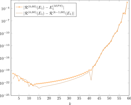
Figure 12: Error over the first eigenvalue of the unit square with a $45^{0}$-crack. The asymptotic series of Eq. (106) has been used.

Table 6: Correct digits of the first 5 eigenvalues of the unit square with a $45^{0}$-crack, obtained by applying the Richardson and Richardson-Padé extrapolations to FD eigenvalues.

$n$	$\log_{10}\frac{1}{|E_{n}^{({\rm RE})}-E_{n}^{\rm(MPS)}|}$	$\log_{10}\frac{1}{|E_{n}^{({\rm PRE})}-E_{n}^{\rm(MPS)}|}$
1	22.18	25.37
2	23.65	23.87
3	22.00	23.92
4	21.04	24.22
5	20.85	23.01

It is interesting to check the numerical values obtained for the coefficients of the series (106), using the Richardson extrapolation of the FD results corresponding to the last 30 grids, for the modes above:

$$E_{1}(h) \approx 35.63151952+22.47641559\ h^{8/7}-71.03523727\ h^{2}+6.078713368\ h^{16/7}$$ (107)

$$- 78.46323288\ h^{22/7}-8.840565052\ h^{24/7}+63.35756993\ h^{4}+\dots$$

$$E_{2}(h) \approx 54.19310844-2.87\times 10^{-17}\ h^{8/7}-164.3992546\ h^{2}-21.20457267\ h^{16/7}$$ (108)

$$+ 1.03\times 10^{-8}\ h^{22/7}-1.44\times 10^{-7}\ h^{24/7}+212.7295338\ h^{4}+\dots$$

$$E_{3}(h) \approx 73.63330813+3.52\times 10^{-17}\ h^{8/7}-260.5413126\ h^{2}+8.56\times 10^{-12}\ h^{16/7}$$ (109)

$$- 3.15\times 10^{-8}\ h^{22/7}-91.25393089\ h^{24/7}+222.794824\ h^{4}+\dots$$

$$E_{4}(h) \approx 104.3280905-2.12\times 10^{-15}\ h^{8/7}-668.8593013\ h^{2}-3.38\times 10^{-10}\ h^{16/7}$$ (110)

$$+ 9.07\times 10^{-7}\ h^{22/7}-39.10703889\ h^{24/7}+1997.967306\ h^{4}+\dots$$

$$E_{5}(h) \approx 124.5914636-2.6\times 10^{-15}\ h^{8/7}-766.4031071\ h^{2}-13.2187842\ h^{16/7}$$ (111)

$$+ 1.17\times 10^{-6}\ h^{22/7}-0.00001758167793\ h^{24/7}+1901.063425\ h^{4}+\dots$$

Clearly one observes that depending on the mode chosen, some of the coefficients are consistent with a vanishing value: these observations are summarized in Table 7, where the leading rational coefficients and the corresponding reentrant angle are reported for each of the first 5 modes.

Table 7: Leading rational exponents of the FD series for the first 5 modes of the square with a $45^{0}$-crack, and corresponding reentrant angles.

$n$	leading exponent	dominant angle
1	$\frac{8}{7}$	$\frac{7\pi}{4}$
2	$\frac{16}{7}$	$\frac{7\pi}{8}$
3	$\frac{24}{7}$	$\frac{7\pi}{12}$
4	$\frac{24}{7}$	$\frac{7\pi}{12}$
5	$\frac{16}{7}$	$\frac{7\pi}{8}$

4.5 Square domain with two slits

Consider the unit square with two $1/4$ slits, represented in Fig. 13. This example has been studied in Refs. [4, 23]. In this case the re-entrant corner is $2\pi$, thus the leading exponent in the FD series is $\alpha_{1}=1$. Eliminating the pollution of this contribution, Blum and Rannacher were able to obtain $E_{1}=35.728$ for their finest grid.

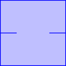
Figure 13: Square domain with two slits

Consistently with our previous assumptions, we conjecture that the FD series has the form

$$E^{(k)}=c_{0}+\sum_{j=1}^{\infty}c_{j}h_{k}^{j}$$ (112)

which is the typical form used in Richardson extrapolation. In this case, Bender and Orszag provide in [2] a nice explicit formula for the coefficient $c_{0}$ (Eq.(8.1.16) of pag. 375 of their book), which in our notation reads:

$$c_{0}=\sum_{k=0}^{N}\frac{E^{(n+k)}(n+k)^{N}(-1)^{k+N}}{k!(N-k)!}$$ (113)

Our numerical experiments with this domain consist of two sets:

• a set which contains the numerical approximation to the lowest eigenvalue of the domain calculated to 220 digits of accuracy using the CGM, for 36 grids with $h=1/2n$ and $n=8,10,\dots,80$;

• a set which contains the numerical approximation to the lowest 50 eigenvalues of the domain calculated to 60 digits arithmetic using the internal Mathematica command

  igenvalue    for 20 grids with
  $h = 1/2n$ and $n=8, 10, \dots, 46$;
  \end{itemize}
  In table \ref{tab_slit} we report the approximate values of selected eigenvalues of this domain, obtained using
  Richardson and Pad\’e-Richardson extrapolation. The eigenvalue of the fundamental mode is obtained using the
  first set of FD results, whereas the remaining eigenvalues are obtained using the second set.
  The digits reported in the table are believed to be correct. The table omits the  eigenmodes
  of the square, for which the convergence is much faster.
  \begin{table}[!htbp]
  \caption{Selected eigenvalues of the square with two slits obtained using Richardson and Pad\’e-Richardson extrapolation
  of the FD results}
  \bigskip
  \label{tab_slit}
  \begin{center}
  \begin{tabular}{|c|l|l|}
  \hline
  $n$ & $

  _n^(R)$&$E_n^(PR)$\\ {\hline}128.13136748084575475520628.131367480845754755206268\\ 370.6503847036870.65038470368488\\ 599.84675925389599.8467592538950\\ 7130.483305932580130.4833059325804\\ 8153.39663535893153.3966353589373\\ 10196.598428600514196.5984286005142\\ 13218.04116455831218.0411645583168\\ 15268.2038796851519268.2038796851519\\ 16272.5993876495272.59938764953\\ 17280.750584654280.7505846542989\\ 20348.460286264284348.4602862642840\\ 50750.8475130750.847513086\\ {\hline}$

  
  

Of particular interest is the fiftieth mode, whose nodal lines are the solid lines displayed in Figs. 14. Looking at the left plot, we are tempted to assume that a nodal line partitions each of the $2\pi$ reentrant angles into three angles of $2\pi/3$, which would imply that the corresponding FD series would now have rational exponents. A simple analysis of the FD results however shows that this mode is also described by the series in eq. (112). This behavior is consistent with the information delivered by the right plot in Figs. 14, that reveals that in fact the nodal line do not end in the reentrant corner. In other words, the study of the FD series for a given domain, can also provide information on the behavior of the nodal lines of the corresponding eigenmodes.

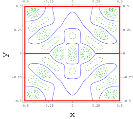
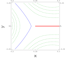
Figure 14: Nodal lines of the $50^{\rm th}$ mode of the square domain with two slits.

5 Conclusions

In this paper we have showed that it is possible to obtain precise estimates for the eigenvalues of the negative Laplacian over particular domains in the plane by performing a Richardson extrapolation or a rational (Padé)-Richardson extrapolation of the results obtained with finite differences, where the exponents of the series are related to the reentrant angles in the domain. The problem of determining the series describing the behavior of the finite difference results from first principles is difficult and it seems that a theoretical study is still lacking. The problem is both challenging and interesting for the applications of finite differences in Physics, Applied Mathematics and Engineering are as numerous as the stars in the Milky Way. Quoting Kuttler and Sigillito, pag. 178 of [21], ”the exact form of the first several terms in the asymptotic formula for specific regions where no boundary interpolation is required is a nice problem at about the level of a doctoral thesis.” The fact that, since 1984 this problem has not been yet solved suggests an even higher level of difficulty.

In this paper we have pursued the less ambitious goal of identifying the series (i.e. the exponents) empirically and we have obtained particularly encouraging results. In the case of the L-shaped domain, for instance, the extrapolation of the results obtained with finite differences leads to a determination of the first 68 digits of the lowest eigenvalue.

The knowledge of the finite difference series for a given domain allows a precise determination of the numerical values of the eigenvalues of that domain, making the finite difference method a powerful computational tool .

Here we stress the most relevant observations obtained from a careful analysis of the numerical results for the examples considered in this paper:

• The FD series appears to be an asymptotic series, as suggested by the particular behavior of the error; this does not limit the accuracy of the extrapolated results, if the largest spacing of the set is appropriately decreased, as more and more terms are added;

• The example of the square with a $45^{0}$ crack tells us that when a nodal line terminates in a reentrant corner, the corresponding FD series have exponents corresponding to the fractions of reentrant angles, even if the nodal line is not completely sampled by the grid (it is the behavior infinitesimally close to the corner that matters);

• It is reasonable to assume that, for a given domain, the FD series corresponding to the different modes all are described by the same series (although for some modes some exponents could be missing for symmetry reasons – this is the case of the modes of the L which are also eigenmodes of the square, for which all the coefficients of all rational exponents vanish );

• If the observation above is correct, this means that one cannot have nodal lines partitioning the reentrant corner if the new exponent generated is not of the type already contained in the series! The case of the fiftieth mode of the square with two slits illustrates this behavior: the nodal lines stretch almost completely to the reentrant corner, although they do not join it!

• We conjecture that the nature of the reentrant corners fully determines the exponents of the FD series and therefore different domains, containing the same reentrant angles should all have the same exponents (see for example the case of the L, of the H and of the isospectral domains considered in this paper); this makes Richardson (and Richardson-Padé) extrapolation practical even for complicated domains where the use of MPS can be problematic;

• For the case of the L-shape and of the square with a $45^{0}$ crack, our results also provide an independent check/validation of the corresponding results obtained using MPS;

References

- [1] P. Amore, Solving the helmholtz equation for membranes of arbitrary shape: numerical results, J. Phys. A, 41 (2008), p. 265206.
- [2] C. M. Bender and S. A. Orszag, Advanced Mathematical Methods for Scientists and Engineers I, Springer Science & Business Media, 1999.
- [3] T. Betcke and L. N. Trefethen, Reviving the method of particular solutions, Siam Review, 47 (2005), pp. 469–491.
- [4] H. Blum and R. Rannacher, Finite element eigenvalue computation on domainswitch reentrant corners using Richardson extrapolation, J. Comput. Math., 8 (1990), pp. 321–332.
- [5] K. Bohmer and H. J. Stetter, eds., Defect Corection Methods. Theory and Applications, Springer, New York, 1984.
- [6] J. P. Boyd, Chebyshev and Fourier Spectral Methods, Dover, New York, 2001. 680 pp.
- [7] C. Brezinski, Extrapolation algorithms and Padé approximations: a historical survey, Appl. Numer. Math., 20 (1996), pp. 299–318.
- [8] E. Christiansen and H. G. Petersen, Estimation of convergence orders in repeated Richardson extrapolation, BIT, 29 (1989), pp. 48–59.
- [9] K. W. Chu and A. Spence, Deferred correction for the integral equation eigenvalue problem, Bull. Australian Math. Soc., 22 (1981), pp. 474–487.
- [10] J. Donnelly, Eigenvalues of membranes with reentrant corners, Siam Review, 6 (1969), pp. 163–193.
- [11] T. A. Driscoll, Eigenmodes of isospectral drums, Siam Review, 39 (1997), pp. 1–17.
- [12] A. Dutt, L. Greengard, and V. Rokhlin, Spectral deferred correction methods for ordinary differential equations, BIT, 40 (2000), pp. 241–266.
- [13] L. Fox, Some improvements in the use of relaxation methods for the solution of ordinary and partial differential equations, Proc. Roy. Soc. London A, 190 (1947), pp. 31–59.
- [14] L. Fox, P. Henrici, and C. Moler, Approximations and bounds for eigenvalues of elliptic operators, Siam Journal on Numerical Analysis, 4 (1967), pp. 89–102.
- [15] O. Giraud and K. Thas, Hearing shapes of drums: Mathematical and physical aspects of isospectrality, Rev. Mod. Phys., 82 (2010), p. 2213.
- [16] C. Gordon, D. Webb, and S. Wolpert, Isospectral plane domains and surfaces via riemannian orbifolds, Invent. Math., 110 (1992), p. 1.
- [17] , One cannot hear the shape of a drum, Bull. Am. Math. Soc., 27 (1992), p. 134.
- [18] J. Huang, J. Jia, and M. Minion, Accelerating the convergence of spectral deferred correction methods, J. Comput. Phys., 214 (2006), pp. 633–656.
- [19] J. Jia, J. C. Hill, K. J. Evans, G. I. Fann, and M. A. Taylor, A spectral deferred correction applied to the shallow water equations on a sphere, Monthly Weather Rev., 141 (2013), pp. 3435–3449.
- [20] D. C. Joyce, Survey of extrapolation processes in numerical analysis, SIAM Rev., 11 (1970), pp. 435–488.
- [21] J. Kuttler and V. Sigillito, Eigenvalues of the laplacian in two dimensions, Siam Review, 26 (1984), pp. 163–193.
- [22] A. T. Layton and M. L. Minion, Implications of the choice of quadrature nodes for Picard integral deferred corrections methods for ordinary differential equations, BIT, 45 (2005), pp. 341–373.
- [23] H. Liu and J. Sun, Recovery type a posteriori estimates and superconvergence for nonconforming fem of eigenvalue problems, Applied Mathematical Modelling, 33 (2009), pp. 3488–3497.
- [24] G. I. Marchuk and V. V. Shaidurov, Difference Methods and Their Extrapolations, Springer-Verlag, New York, 1983. 334 pp.
- [25] J. Mason, Chebyshev polynomial approximations for the l-membrane eigenvalue problem, SIAM J. Appl. Math., 15 (1967), p. 172.
- [26] M.P.Nightingale, V. Viswanath, and G. Muller, Computation of dominant eigenvalues and eigenvectors: a comparative study of algorithms, Phys. Rev. B, 48 (1993), pp. 7696–7699.
- [27] J. D. Pryce, Numerical Solution of Sturm-Liouville Problems, Clarendon Press, Oxford U. Press, Oxford, 1993. 336 pp.
- [28] J. Reid and J. Walsh, An elliptic eigenvalue problem for a reentrant region, Journal of the Society for Industrial and Applied Mathematics, 13 (1965), pp. 837–850.
- [29] L. F. Richardson, The deferred approach to the limit. Part I.— Single lattice, Philosophical Transactions of the Royal Society, 226 (1927), pp. 299–349.
- [30] H. E. Salzer, A simple method for summing certain slowly converging series, J. Math. Phys., 33 (1954), pp. 356–359.
- [31] B. Schiff, Finite element eigenvalues for the laplacian over an l-shaped domain, J. Comp. Phys, 76 (1988), pp. 233–242.
- [32] A. Sideridis, A numerical solution of the membrane eigenvalue problem, Computing, 32 (1984), pp. 167–176.
- [33] A. Sidi, Practical Extrapolation Methods: Theory and Applications, vol. 10 of Cambridge Monographs on Applied and Computational Mathematics, Cambridge University Press, New York, 2002.
- [34] S. Sridhar and A. Kudrolli, Experiments on not hearing the shape of drums, Phys. Rev. Lett., 72 (1994), p. 2175.
- [35] G. Still, Approximation theory methods for solving elliptic eigenvalue problems, Z. Angew. Math. Mech., 83 (2003), pp. 469–478.
- [36] K. wah Eric Chu, Deferred correction for the ordinary differential equation eigenvalue problem, Bull. Australian Math. Soc., 26 (1982), pp. 445–454.
- [37] G. Walz, Asymptotics and extrapolation, Wiley-VCB, Berlin, 1996. 333 pp.
- [38] I. Wolfram Research, Mathematica, Wolfram Research, Inc., Champaign, Illinois, 2015. .
- [39] H. Wu, D. Sprung, and J. Martorell, Numerical investigation of isospectral cavities built from triangles, Phys. Rev. E, 51 (1995), pp. 703–708.
- [40] Q. Yuan and Z. He, Bounds to eigenvalues of the laplacian on l-shaped domain by variational methods, Journal of Computational and Applied Mathematics, 233 (2009), pp. 1083–1090.