The magnetic field of $\zeta$ Ori A

Abstract

Context. $\zeta$ Ori A is a hot star claimed to host a weak magnetic field, but no clear magnetic detection was obtained so far. In addition, it was recently shown to be a binary system composed of a O9.5I supergiant and a B1IV star.

Aims. We aim at verifying the presence of a magnetic field in $\zeta$ Ori A, identifying to which of the two binary components it belongs (or whether both stars are magnetic), and characterizing the field.

Methods. Very high signal-to-noise spectropolarimetric data were obtained with Narval at the Bernard Lyot Telescope (TBL) in France. Archival HEROS, FEROS and UVES spectroscopic data were also used. The data were first disentangled to separate the two components. We then analyzed them with the Least-Squares Deconvolution (LSD) technique to extract the magnetic information.

Results. We confirm that $\zeta$ Ori A is magnetic. We find that the supergiant component $\zeta$ Ori Aa is the magnetic component: Zeeman signatures are observed and rotational modulation of the longitudinal magnetic field is clearly detected with a period of 6.829 d. This is the only magnetic O supergiant known as of today. With an oblique dipole field model of the Stokes V profiles, we show that the polar field strength is $\sim$140 G. Because the magnetic field is weak and the stellar wind is strong, $\zeta$ Ori Aa does not host a centrifugally supported magnetosphere. It may host a dynamical magnetosphere. Its companion $\zeta$ Ori Ab does not show any magnetic signature, with an upper limit on the undetected field of $\sim$ 300 G.

1 Introduction

Magnetic fields play a significant role in the evolution of hot massive stars. However, the basic properties of the magnetic fields of massive stars are poorly known. About 7% of the massive stars are found to be magnetic at a level that is detectable with current instrumentation (Wade et al. 2014). In particular, only 11 magnetic O stars are known. Detecting magnetic field in O stars is particularly challenging because they only have few, often broad, lines from which to measure the field. There is therefore a deficit in the knowledge of the basic magnetic properties of O stars.

We here study the O star $\zeta$ Ori A. A magnetic field seems to have been detected in this star by Bouret et al. (2008). Their detailed spectroscopic study of the stellar parameters led to the determination of an effective temperature of $T_{\rm eff}$ = 29500 $\pm$ 1000 K and log g = 3.25 $\pm$ 0.10 with solar abundances. This makes $\zeta$ Ori A the only magnetic O supergiant. Moreover, Bouret et al. (2008) found a magnetic field of 61 $\pm$ 10 G, which makes it the weakest ever reported field in a hot massive star (typically ten times weaker than those detected in other magnetic massive stars). They found a rotational period of $\sim$7 days from the temporal variability of spectral lines and the modulation of the Zeeman signatures. To derive the magnetic properties, they used six lines that are not or only weakly affected by the wind. The rotation period they obtained is compatible with their measured $v\sin{i}$=100 km s^-1.

In addition, the measurement of the magnetic field provided by Bouret et al. (2008) allows characterizing the magnetosphere of $\zeta$ Ori A and locating it in the magnetic confinement-rotation diagram (Petit et al. 2013): $\zeta$ Ori A is the only known magnetic massive star with a confinement parameter below 1, that is, without a magnetosphere.

For all these reasons, the study of the magnetic field of $\zeta$ Ori A is of the highest importance. Each massive star that is detected to be magnetic moves us closer to understanding the stellar magnetism of hot stars. Studying this unique magnetic massive supergiant is also of particular relevance for our understanding of the evolution of the magnetic field in hot stars.

$\zeta$ Ori A has a known B0III companion, $\zeta$ Ori B. In addition, Hummel et al. (2013) found that $\zeta$ Ori A consists of two companion stars located at 40 mas of each other, orbiting with a period of 2687.3$\pm$7.0 days. To determine a dynamical mass of the components, Hummel et al. (2013) analyzed archival spectra to measure the radial velocity variations. The conclusions reached are presented below. The primary $\zeta$ Ori Aa is a O9.5I supergiant star, whose radius is estimated to 20.0$\pm$3.2 $R_{\odot}$ and whose mass is estimated to 33$\pm$10 $M_{\odot}$. The secondary $\zeta$ Ori Ab is a B1IV with an estimated radius of 7.3$\pm$1.0 $R_{\odot}$ and an estimated mass of 14$\pm$3 $R_{\odot}$. Moreover, $\zeta$ Ori A is situated at a distance of 387 pc. Initial estimates of the elements of the apparent orbit were obtained by Hummel et al. (2013) using the Thiele-Innes method. The estimation provided a value of the periastron epoch of JD 2452734.2$\pm$9.0 with a longitude of 24.2$\pm$1.2^∘. The eccentricity is estimated to be 0.338$\pm$0.004.

Bouret et al. (2008) considered $\zeta$ Ori A as a single star of 40 $M_{\odot}$ with a radius equal to 25 $R_{\odot}$, seen from Earth at an inclination angle of 40^∘. Taking into account that the star is a binary could strongly modify the magnetic field value derived for only one of the binary components. In their analysis, the magnetic signature was normalized by the full intensity of the lines from both components, and if only one of the two stars is magnetic, the field was thus underestimated. Moreover, the position in the magnetic confinement-rotation diagram will be modified as a result of the new magnetic strength value, but also as a consequence of the new stellar parameters.

Based on new spectropolarimetric observations of $\zeta$ Ori A and archival spectra presented in Sect. 2, we here seek to confirm that $\zeta$ Ori A is a magnetic star (Sect. 3). We determine with several techniques, including by disentangling the composite spectrum (Sect. 4) whether the magnetic field is hosted by the primary or the secondary star of $\zeta$ Ori A. We then determine the field strength of the magnetic component (Sect. 5) and quantify the non-detection of a field in the companion (Sect. 6). In addition, we investigate the rotational modulation of the magnetic field, its configuration (Sect. 7), and the possible presence of a magnetosphere (Sect. 8). Finally, we discuss our results and draw conclusions in Sect. 9.

2 Observations

2.1 Narval spectropolarimetric observations

Table 1: Journal of Narval observations. The columns list the date and the heliocentric Julian date (HJD) for the middle of observation, the number of sequences, and the exposure time per individual subexposure, the signal-to-noise ratio in the I profiles, and the orbital phase.

#	Date	mid-HJD	$T_{exp}$ (s)	S/N	$\phi_{\rm orb}$
1	17oct07	2454391.559	48 $\times$ 4 $\times$ 20	4750	0.617
2	18oct07	2454392.719	8 $\times$ 4 $\times$ 40	2220	0.617
3	19oct07	2454393.570	44 $\times$ 4 $\times$ 40	6940	0.617
4	20oct07	2454394.491	48 $\times$ 4 $\times$ 40	6860	0.618
5	21oct07	2454395.518	48 $\times$ 4 $\times$ 40	7070	0.618
6	23oct07	2454397.496	48 $\times$ 4 $\times$ 40	7180	0.619
7	24oct07	2454398.526	48 $\times$ 4 $\times$ 40	7270	0.619
8	22oct08	2454762.644	40 $\times$ 4 $\times$ 50	6660	0.755
9	23oct08	2454763.645	38 $\times$ 4 $\times$ 50	5530	0.755
10	24oct08	2454764.654	36 $\times$ 4 $\times$ 50	6790	0.756
11	25oct08	2454765.639	37 $\times$ 4 $\times$ 50	6140	0.756
12	26oct08	2454766.635	38 $\times$ 4 $\times$ 50	6420	0.756
13	04oct11	2455839.688	12 $\times$ 4 $\times$ 90	5810	0.156
14	05oct11	2455840.670	12 $\times$ 4 $\times$ 90	5790	0.156
15	10oct11	2455845.608	12 $\times$ 4 $\times$ 90	2040	0.158
16	11oct11	2455846.632	12 $\times$ 4 $\times$ 90	3450	0.158
17	30oct11	2455865.712	12 $\times$ 4 $\times$ 90	5610	0.165
18	07nov11	2455873.557	5 $\times$ 4 $\times$ 90	2700	0.168
19	11nov11	2455877.626	12 $\times$ 4 $\times$ 90	4860	0.170
20	12nov11	2455878.565	12 $\times$ 4 $\times$ 90	4830	0.170
21	24nov11	2455890.673	12 $\times$ 4 $\times$ 90	4180	0.175
22	25nov11	2455891.660	12 $\times$ 4 $\times$ 90	4900	0.175
23	26nov11	2455892.502	12 $\times$ 4 $\times$ 90	4490	0.175
24	29nov11	2455895.667	12 $\times$ 4 $\times$ 90	5400	0.176
25	30nov11	2455896.600	6 $\times$ 4 $\times$ 90	2030	0.177
26	14dec11	2455910.477	12 $\times$ 4 $\times$ 90	1360	0.182
27	08jan12	2455935.555	12 $\times$ 4 $\times$ 90	5630	0.191
28	13jan12	2455940.536	12 $\times$ 4 $\times$ 90	5060	0.193
29	14jan12	2455941.539	12 $\times$ 4 $\times$ 90	5350	0.193
30	15jan12	2455942.475	12 $\times$ 4 $\times$ 90	4680	0.194
31	16jan12	2455943.367	12 $\times$ 4 $\times$ 90	4520	0.194
32	25jan12	2455952.529	12 $\times$ 4 $\times$ 90	5120	0.198
33	26jan12	2455953.431	8 $\times$ 4 $\times$ 90	3200	0.198
34	08feb12	2455966.472	12 $\times$ 4 $\times$ 90	3900	0.203
35	09feb12	2455967.402	11 $\times$ 4 $\times$ 120	4340	0.203
36	10feb12	2455968.343	12 $\times$ 4 $\times$ 90	2198	0.203

Spectropolarimetric data of $\zeta$ Ori A were collected with Narval in the frame of the project Magnetism in Massive Stars (MimeS) (see e.g. Neiner et al. 2011). This is the same instrument with which the magnetic field of $\zeta$ Ori A was discovered by Bouret et al. (2008). Narval is a spectropolarimeter installed on the two-meter Bernard Lyot Telescope (TBL) at the summit of the Pic du Midi in the French Pyrénées. This fibre-fed spectropolarimeter (designed and optimized to detect stellar magnetic fields through the polarization they generate) provides complete coverage of the optical spectrum from 3700 to 10500 $\AA$ on 40 echelle orders with a spectral resolution of $\sim$65000. Considering the size of the fiber, the light from $\zeta$ Ori B was not recorded in the spectra, but light from both components of $\zeta$ Ori A was collected.

$\zeta$ Ori A was first observed in October 2007 during 7 nights (PI: J.-C. Bouret) and these data were used in Bouret et al. (2008). Then, this star was observed again in October 2008 during 5 nights (PI: J.-C. Bouret) and between October 2011 and February 2012 during 24 nights by the MiMeS collaboration (PI: C. Neiner). This provides a total number of 36 nights of observations. The observations were taken in circular polarimetric mode, that is, measuring Stokes V. Each measurement was divided into four subexposures with a different polarimeter configuration.

Since $\zeta$ Ori A is very bright (V=1.77), only a very short exposure time could be used to avoid saturation. To increase the total signal-to-noise ratio (S/N), we thus obtained a number of successive measurements each night, which were co-added. The exposure time of each subexposure of each measurement varies between 20 and 120 s, and the total integration time for a night varies between 1280 and 7680 s (see Table 1).

Data were reduced at the telescope using the Libre-Esprit reduction package (Donati et al. 1997). We then normalized each of the 40 echelle orders of each of the 756 spectra with the continuum task of IRAF. Finally, we co-added all the spectra obtained within each night to improve the S/N, which varies between 1360 and 7270 in the intensity spectra (see Table 1). We therefore obtained 36 nightly averaged measurements.

2.2 Archival spectroscopic observations

Figure 1: LSD Stokes I (bottom), Stokes V (top), and null N (middle) profiles, normalized to Ic, for 8 selected nights. The red line is a smoothed profile.

In addition to the spectropolarimetric data, we used archival spectroscopic data of $\zeta$ Ori A taken with various echelle spectrographs.

In 1995, 1997 and 1999, spectra were obtained with the HEROS instrument, installed at the ESO Dutch 0.9 m telescope at the La Silla Observatory. The spectral resolution of HEROS is 20000, with a spectral domain from about 350 to 870 nm. In addition, in 2006, 2007 and 2009, data were taken with the FEROS spectrograph installed at the ESO 2.2 m at the La Silla observatory. The spectral resolution of FEROS is about 48000 and the spectral domain ranges from about 370 to 900 nm. Finally, in 2010, spectra were taken with the UVES spectrograph (Dekker et al. 2000) installed at the VLT at the Paranal Observatory. Its spectral domain ranges from about 300 to 1100 nm with a spectral resolution of 80000 and 110000 in the blue and red domains respectively.

We co-added spectra collected for each year to improve the final S/N. We therefore have seven spectra for seven different years, with a S/N of between about 100 and 2000 (see Table 2).

Table 2: Journal of archival spectroscopic observations of $\zeta$ Ori A obtained with HEROS, FEROS and UVES, showing the date and heliocentric Julian date, instrument used, exposure time, signal-to-noise ratio, and orbital phase.

Date	JD	Instrument	Texp	S/N	$\phi_{\rm orb}$
1995	2449776.024	HEROS	57$\times$1200	1200	0.90
1997	2450454.379	HEROS	16$\times$1200	1000	0.15
1999	2451147.333	HEROS	64$\times$1200	1200	0.41
2006	2453738.159	FEROS	60	100	0.37
2007	2454501.018	FEROS	2$\times$20	250	0.66
2009	2454953.970	FEROS	5$\times$10	200	0.84
2010	2455435.373	UVES	36$\times$2	2000	0.01

3 Checking for the presence of a magnetic field

The magnetic field of $\zeta$ Ori A claimed by Bouret et al. (2008) has not been confirmed by independent observations so far and one of the goals of this study is to confirm or disprove its existence using additional observations.

To test whether $\zeta$ Ori A is magnetic, we applied the Least-Squares Deconvolution (LSD) technique (Donati et al. 1997). We first created a line mask for $\zeta$ Ori A. We started from a list of lines extracted from VALD (Piskunov et al. 1995; Kupka & Ryabchikova 1999) for an O star with $T_{\rm eff}$=30000 K and log g=3.25, with their Landé factors and theoretical line depths. We then cleaned this line list by removing the hydrogen lines, the lines that are blended with hydrogen lines, and those that are not visible in the spectra. We also added some lines visible in the spectra that were not in the original O-star mask. Altogether, we obtained a mask of 210 lines. We then adjusted the depth of these 210 lines in the mask to fit the observed line depths.

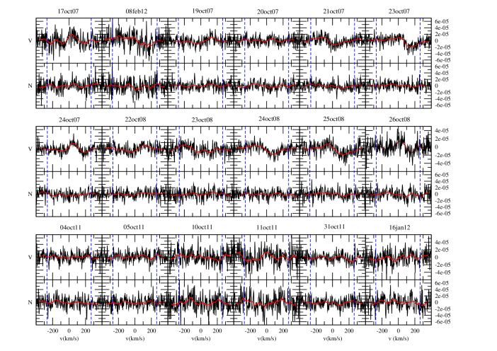
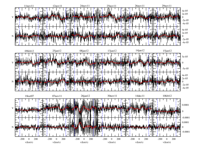
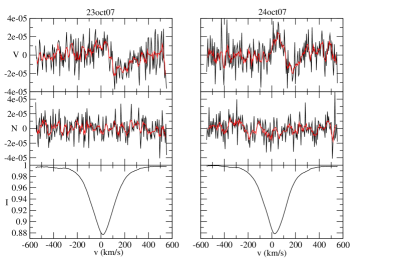
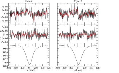
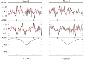
Using the final line mask, we extracted LSD Stokes I and V profiles for each night. We also extracted null (N) polarization profiles to check for spurious signatures. The LSD I, Stokes V and the null N profiles are shown in Fig. 1 for 8 of 36 nights. A plot of all profiles is available online (Fig. 11). Zeeman signatures are clearly seen for these 8 nights and some others as well, but are not systematically observed for all nights. We calculated the false alarm probability (FAP) by comparing the signal inside the lines with no signal (Donati et al. 1997). If FAP $<$ 0.001%, the magnetic detection is definite; if it is 0.001% $<$ FAP $<$ 0.1% the detection is marginal, otherwise there is no detection. Table 3 indicates whether a definite detection (DD), marginal detection (MD) or no detection (ND) was obtained for each of the night. DD or MD were obtained in 15 out of 36 nights. The existence of Zeeman signatures confirms that $\zeta$ Ori A hosts a magnetic field, as previously reported by Bouret et al. (2008).

The previous study of the magnetic field of $\zeta$ Ori A (Bouret et al. 2008) only used a few lines that were not affected by the wind. However, we need to use as many lines as possible to improve the S/N. We therefore checked whethe our results were changed by using lines that might be affected by the wind. We compared the LSD results obtained with the mask used by Bouret et al. (2008) and our own mask (see Fig. 2). The signatures in Stokes V are similar with both masks and the measurements of the longitudinal magnetic field are consistent (e.g., 44.5$\pm$19.6 G with the mask of Bouret et al. (2008) and 35.8$\pm$7.2 G with our mask for measurement # 11, see Fig. 2). However, the S/N is better with our mask (the S/N of Stokes V is 57624) than with the mask of Bouret et al. (2008) (the S/N of Stokes V is 27296). Therefore, we used all available lines for this study.

However, the line mask used in this first analysis includes lines from both components of $\zeta$ Ori A. We thus ignored which component of the binary is magnetic or whether both components are magnetic. To provide an answer to this question, we must separate the composite spectra.

Figure 2: LSD Stokes I (bottom), Stokes V (top), and null N (middle) profiles, normalized to Ic, for the night of 25 October 2008 for the mask of Bouret et al. (2008) (left) and for our own mask (right). The red line is a smoothed profile.

4 Separating the two components

4.1 Identifying the lines of each component

We first created synthetic spectra of each component. The goal was to identify which lines come from the primary component, the secondary component, or both. To this aim, we used TLUSTY (Hubeny & Lanz 1995). This program calculates plane-parallel, horizontally homogeneous stellar atmosphere models in radiative and hydrostatic equilibrium. One of the most important features of the program is that it allows for a fully consistent, non-LTE metal line blanketing. However, TLUSTY does not take winds into account, which can be important in massive stars, especially in supergiants.

For the primary component $\zeta$ Ori Aa, we computed a model with an effective temperature $T_{\rm eff}$=29500 K and logg=3.25, corresponding to the spectral type of the primary as given by Hummel et al. (2013). For the secondary, we computed a model with an effective temperature $T_{\rm eff}$=29000 K et logg=4.0, again following Hummel et al. (2013). We used solar abundances, for both stars. The emergen spectrum from a given model atmosphere was calculated with SYNSPEC. This program is complemented by the program ROTINS, which calculates the rotational and instrumental convolutions for the net spectrum produced by SYNSPEC.

Comparing these two synthetic spectra to the observed spectra of $\zeta$ Ori A, we identified which lines belong only to $\zeta$ Ori Aa, only to $\zeta$ Ori Ab, and which are a blend of the lines of both components. If one observed line only existed in one synthetic spectrum, we considered that this line is only emitted from one component of the binary. If it existed in both synthetic spectra, we considered this line to be a blend of both components. We then created line lists containing lines from the three categories (only Aa, only Ab, or both).

In addition, we gathered archival spectra of $\zeta$ Ori A taken with the spectrographs FEROS, HEROS and UVES (see Sect. 2.2). While these spectra do not include polarimetric information, they cover the orbital period much better than our Narval data (see Table 2 and Fig. 3). In particular, some spectra were obtained close to the maximum or minimum of the radial velocity (RV) curve.

We compared the spectrum taken close to the maximum and minimum RV, because the line shift is maximum between these two spectra. We arbitrarily decided to use the spectra taken close to the maximum as reference. Depending on the shift, we determined the origin of the lines. If the lines of the spectrum taken at minimum RV are shifted to the blue (respectively red) side compared to the spectrum at maximum RV, the line comes from the primary Aa (respectively secondary Ab) component. When lines from the two components are blended, the core of the lines are shifted to the red side and the wings to the blue side.

The identification of lines made this way resulted in similar line lists as those obtained by comparing the observed spectra with synthetic ones.

We then ran LSD again on the observed Narval spectra, once with the mask containing the 157 lines only belonging to $\zeta$ Ori Aa and once with the mask only containing the 67 lines from $\zeta$ Ori Ab. We observe magnetic signatures in the LSD V profiles of $\zeta$ Ori Aa that are similar to those obtained in the original LSD analysis presented in Sect. 3. In the contrast, we do not observe magnetic signatures in the LSD Stokes V profiles of $\zeta$ Ori Ab. We conclude that $\zeta$ Ori Aa is magnetic and $\zeta$ Ori Ab is not.

However, the LSD profiles of $\zeta$  Ori Aa obtained this way are very noisy, because of the low number of lines in the mask, and they cannot be used to precisely estimate the longitudinal magnetic field strength. To go further, it is necessary to disentangle the spectra, so that more lines can be used.

4.2 Spectral disentangling of Narval data

We first attempted to use the Fourier-based formulation of the spectral disentangling (hereafter, spd) method (Hadrava 1995) as implemented in the FDBinary code (Ilijic et al. 2004) to simultaneously determine the orbital elements and the individual spectra of the two components Aa and Ab of the $\zeta$ Ori A binary system. The Fourier-based spd method is superior to the original formulation presented by Simon & Sturm (1994) that is applied in the wavelength domain in that it is less time-consuming. In particular, this increases the technique’s efficiency when it is applied to long time-series of high-resolution spectroscopic data.

One of the pre-conditions for the spd method to work efficiently is a homogeneous phase coverage of the orbital cycle with the data. In particular, covering the regions of maximum/minimum radial velocity (RV) separation of the two stars is essential, because these phases provide key information about the RV semi-amplitudes of both stellar components.

Figure 3 illustrates the phase distribution of our Narval spectra according to the orbital period of 2687.3 days reported by Hummel et al. (2013). Obviously, the spectra provide very poor phase coverage; no measurements exist at phases $\sim$0.0 and 0.4, corresponding to a maximum RV separation of the components (see Fig. 5 in Hummel et al. 2013). This prevents determining of accurate orbital elements from our Narval spectra.

Our attempt to use the orbital solution obtained by Hummel et al. (2013) to separate the spectra of the individual components also failed: although all regions in which we disentangled the spectra indicate the presence of lines from the secondary in the composite spectra, the separated spectra themselves are unreliable.

Figure 3: Orbital phase distribution of the spectra of $\zeta$ Ori A. The diamonds indicate the radial velocity measured by Hummel et al. (2013). The lines correspond to the best fit of the radial velocity of each component. The crosses correspond to our Narval observations and the triangles to the archival spectroscopic data. Phase zero corresponds to the time of periastron passage (T₀ = 2452734.2 HJD) as reported by Hummel et al. (2013).

4.3 Disentangling using the archival spectroscopic data

Since the spd method failed in disentangling the Narval spectra because of the poor phase coverage, we again used the spectroscopic archival data obtained with FEROS, HEROS, and UVES. The orbital coverage of these spectra is much better than the one of the Narval data. We have seven spectra taken at different orbital phases, including phases of maximum RV separation of the components (see Table 3). We first normalized the spectra with IRAF. We used the orbital parameters given by Hummel et al. (2013) for the disentangling.

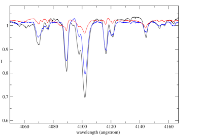
The coverage of these spectra enables the disentangling using FDBinary. As an illustration of the results, a small part of the disentangled spectra is shown in Fig. 4. The results confirms the origin of the lines that were determined in Sect.4.1, and also the spectral types of the components given by Hummel et al. (2013).

5 Measuring the longitudinal magnetic field of $\zeta$ Ori Aa

Following these results, we assume that $\zeta$ Ori Ab is not magnetic and that the Stokes V signal only comes from $\zeta$ Ori Aa. Therefore, we ran the LSD technique on the Narval spectra with a mask containing all lines emitted from $\zeta$ Ori Aa, even those that are blended with the ones of $\zeta$ Ori Ab, to obtain the LSD Stokes V profile of $\zeta$ Ori Aa. The contribution of $\zeta$ Ori Ab to this Stokes V signal will be null, as the magnetic signal is only provided by $\zeta$ Ori Aa.

However, we were unable to disentangle the Narval data (see Sect. 4.2), therefore the LSD Stokes I spectra of $\zeta$ Ori Aa could not be computed in the same way as the LSD Stokes V spectra. As a consequence, we attempted to compute the LSD Stokes I profiles in several ways.

5.1 Using the Narval data and correcting for the companion

For the I profiles, we first proceeded in the following way: we computed the LSD Stokes I profiles with different masks that only contained the lines of $\zeta$ Ori Aa, only the lines of $\zeta$ Ori Ab, and the only blended lines. We subtracted the LSD Stokes I profiles obtained for the lines of $\zeta$ Ori Ab alone from the LSD Stokes I profiles obtained for blended lines to remove the contribution from the Ab component. We then averaged the LSD Stokes I profiles obtained this way and the one obtained for the lines of $\zeta$ Ori Aa alone. In this way the same list of lines (those of Aa alone and the blended ones) are used in the final LSD Stokes I profiles as in the LSD Stokes V profiles calculated above.

This allowed us to use more lines than in Sect. 4.1 (i.e., to include the blended lines) and to improve the resulting S/N. We obtained magnetic signatures similar to those derived in Sects. 3 and 4.1 (see Fig. 1). However, the S/N remained low, and some contribution from the Ab component is probably still present in the LSD Stokes I profile. Longitudinal field values extracted from these LSD profiles may thus be unreliable.

5.2 Using synthetic intensity profiles

To improve the LSD I profiles, we attempted to use the synthetic TLUSTY/SYNSPEC spectra calculated in Sect. 4.1 for $\zeta$ Ori Aa. We ran the LSD tool on the synthetic spectra to produce the synthetic LSD Stokes I profiles of $\zeta$ Ori Aa with the same line mask as the one used for the LSD Stokes V profiles above.

We then computed the longitudinal magnetic field values from the observed LSD Stokes V profiles and the synthetic LSD Stokes I profiles. We calculated the longitudinal magnetic field B_l for all observations with the center-of-gravity method (Rees & Semel 1979),

$$B_{l}=-2.14\times 10^{-11}\frac{\int vV(v)dv}{\lambda_{0}g_{m}c\int(1-I(v))dv}\ G.$$

We obtained longitudinal magnetic field values between -144 and +112 G with error bars between 20 and 100 G.

5.3 Using disentangled spectroscopic data

Although we were unable to disentangle the Narval data, we obtained disentangled spectra from the purely spectroscopic archival data. To derive the longitudinal magnetic field values more accurately, we therefore used the disentangled spectra obtained from the purely spectroscopic data.

Figure 4: Small part of the spectrum of $\zeta$ Ori A showing the composite observed spectrum (black), the spectrum of $\zeta$ Ori Aa (blue) and that of $\zeta$ Ori Ab (red).

We ran the LSD technique on the disentangled archival spectra obtained for $\zeta$ Ori Aa using the same line list as we used for Stokes V. Thus, we obtained the observed mean intensity profile for $\zeta$ Ori Aa alone. We then computed the longitudinal magnetic field values from the observed LSD Stokes V profiles from Narval and the observed LSD Stokes I profiles from the disentangled spectroscopic spectra.

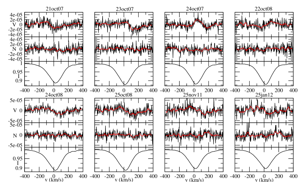
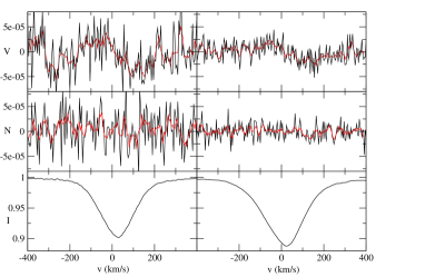
The shape of the magnetic signatures in LSD Stokes V profiles (Fig. 5) is similar to the shapes obtained for the combined spectra (Fig. 1) and the various methods presented above. The LSD Stokes I spectra now better represent the observed $\zeta$ Ori Aa spectrum, however. We therefore adopted these LSD profiles in the remainder of this work. Fifteen of the 36 measurements are DD or MD.

Figure 5: Examples of LSD Stokes I profiles (bottom) computed from the disentangled spectroscopic data, Stokes V (top) and null N (middle) profiles, normalized to Ic, from the Narval data for the primary component $\zeta$ Ori Aa for a few nights of observations. The red line is a smoothed profile.

As above, we calculated the longitudinal magnetic field B_l for all observations with the center-of-gravity method (Rees & Semel 1979). Results are given in Table 3. The longitudinal field B_l varies between about -30 and +50 G, with typical error bars below 10 G. N values are systematically compatible with 0 within 3$\sigma$N, where $\sigma$N is the error on N, while B_l values are above 3$\sigma$B_l in seven instances, where $\sigma$B_l is the error on B_l.

Table 3: Longitudinal magnetic field of the magnetic primary star $\zeta$ Ori Aa. The columns list the heliocentric Julian dates (HJD) for the middle of observation, the longitudinal magnetic field and its error in gauss, the detection status: definite detection (DD), marginal detection (MD) and no detection (ND), and the ”null” polarization and its error in gauss.

#	mid-HJD	Bl	$\sigma$Bl	Detect.	N	$\sigma$N
1	2454391.559	-5.7	7.7	MD	-3.9	7.7
2	2454392.719	-26.9	16.6	ND	37.2	16.6
3	2454393.570	-9.3	5.5	ND	3.6	5.5
4	2454394.491	-0.3	5.4	ND	6.3	5.4
5	2454395.518	18.1	5.2	MD	12.4	5.4
6	2454397.496	25.5	5.1	MD	3.9	5.1
7	2454398.526	4.7	5.1	MD	-3.7	5.1
8	2454762.644	-15.1	5.5	MD	-6.9	5.5
9	2454763.645	12.8	6.6	ND	-5.4	6.6
10	2454764.654	28.0	5.3	MD	3.6	5.3
11	2454765.639	32.8	6.3	DD	11.1	6.3
12	2454766.635	10.9	6.4	MD	12.7	6.4
13	2455839.688	-3.9	6.5	ND	2.9	6.5
14	2455840.670	3.9	6.5	ND	-6.7	6.6
15	2455845.608	21.3	9.4	ND	4.8	9.4
16	2455846.632	-9.7	11.0	ND	-1.8	11.0
17	2455865.712	12.4	6.5	ND	-0.9	6.6
18	2455873.557	25.2	13.5	MD	-3.6	13.5
19	2455877.626	13.6	7.5	ND	-13.5	7.5
20	2455878.565	7.7	7.5	ND	6.8	7.5
21	2455890.673	6.1	8.7	ND	11.0	8.7
22	2455891.660	24.0	7.4	MD	-6.7	7.4
23	2455892.502	6.0	8.1	ND	-11.4	8.1
24	2455895.667	1.3	6.9	ND	-8.0	6.9
25	2455896.600	-22.6	22.3	ND	22.3	22.5
26	2455910.477	4.1	13.8	ND	13.6	13.8
27	2455935.555	-7.2	7.0	MD	4.2	7.0
28	2455940.536	5.9	7.2	ND	-10.1	7.2
29	2455941.539	-3.1	6.8	MD	4.5	6.8
30	2455942.475	-5.3	8.0	ND	-4.4	8.0
31	2455943.367	4.8	8.4	ND	4.3	8.4
32	2455952.529	25.2	7.3	MD	-12.5	7.3
33	2455953.431	72.3	59.1	DD	-60.4	59.1
34	2455966.472	51.0	9.5	MD	-0.3	9.5
35	2455967.402	1.7	8.5	ND	11.3	8.4
36	2455968.343	10.7	16.7	ND	-13.7	16.6

6 No magnetic field in $\zeta$ Ori Ab

6.1 Longitudinal magnetic field values for $\zeta$ Ori Ab

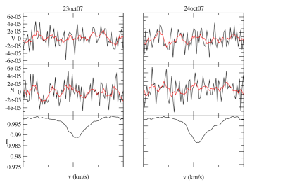
To confirm the non-detection of a magnetic field in $\zeta$ Ori Ab, we ran the LSD technique with a mask that only contained lines emitted from $\zeta$ Ori Ab, that is 67 lines. This ensures that the LSD Stokes V profiles are not polluted by the magnetic field of $\zeta$ Ori Aa. Signatures in the LSD Stokes V profiles are not detected in any of the profiles (all ND), as shown in Table 4 and in Fig. 6 for selected nights when a signal is detected in $\zeta$ Ori Aa.

Figure 6: Examples of LSD Stokes I (bottom), Stokes V (top), and null N (middle) profiles, normalized to Ic, for the secondary component $\zeta$ Ori Ab for a few nights of observations, computed from Narval data using only the 82 lines belonging to the secondary component. The red line is a smoothed profile.

Using these LSD profiles and the center-of-gravity method, we calculated the longitudinal field value, the null polarization, and their error bars for $\zeta$ Ori Ab. We find that both B_l and N are compatible with 0 within 3$\sigma$ for all nights (see Table 4). However, the error bars on the longitudinal field values of $\zeta$ Ori Ab are much higher (typically 70 G) than those for $\zeta$ Ori Aa (typically 10 G), because far fewer lines could be used to extract the signal for $\zeta$ Ori Ab.

Table 4: Longitudinal magnetic field measurements for the secondary $\zeta$ Ori Ab. The columns list the heliocentric Julian dates (HJD) for the middle of observation, the longitudinal magnetic field and its error in gauss, the detection status: no detection (ND) in all cases, and the ”null” polarization and its error in gauss.

#	mid-HJD	Bl	$\sigma$Bl	Detect.	N	$\sigma$N
1	2454391.559	-62.9	74.5	ND	46.5	74.4
2	2454392.719	-80.4	132.7	ND	91.9	132.8
3	2454393.570	26.0	54.8	ND	-60.6	54.9
4	2454394.491	31.0	56.7	ND	24.1	56.6
5	2454395.518	86.7	47.6	ND	101.4	47.7
6	2454397.496	-49.4	45.5	ND	14.3	45.9
7	2454398.526	14.2	46.0	ND	44.6	46.1
8	2454762.644	-14.2	50.8	ND	73.0	50.6
9	2454763.645	-24.1	65.4	ND	43.3	65.5
10	2454764.654	-40.1	49.2	ND	80.0	49.4
11	2454765.639	-32.9	73.5	ND	47.2	73.6
12	2454766.635	7.9	60.5	ND	-26.5	60.6
13	2455839.688	-62.3	53.2	ND	-30.5	53.6
14	2455840.670	-8.3	58.3	ND	3.4	58.2
15	2455845.608	-19.1	92.2	ND	-21.9	91.1
16	2455846.632	-126.4	91.9	ND	-102.1	91.2
17	2455865.712	35.7	63.2	ND	173.4	63.9
18	2455873.557	141.5	112.7	ND	-224.0	113.0
19	2455877.626	55.7	60.0	ND	2.5	60.0
20	2455878.565	34.8	68.3	ND	75.0	68.7
21	2455890.673	-105.9	106.6	ND	-154.9	107.5
22	2455891.660	8.7	82.6	ND	86.6	82.8
23	2455892.502	77.1	84.3	ND	-63.7	84.8
24	2455895.667	-27.0	75.2	ND	-63.8	75.5
25	2455896.600	-33.7	289.4	ND	-113.7	296.7
26	2455910.477	171.0	183.7	ND	129.3	183.4
27	2455935.555	-82.4	70.1	ND	-58.6	69.9
28	2455940.536	-12.3	63.5	ND	-55.8	63.7
29	2455941.539	20.3	67.3	ND	116.9	67.8
30	2455942.475	31.8	70.6	ND	-97.2	71.1
31	2455943.367	-6.2	78.8	ND	-27.7	79.2
32	2455952.529	-72.4	71.0	ND	1.1	71.3
33	2455953.431	173.6	478.5	ND	-152.6	480.7
34	2455966.472	52.9	79.9	ND	-32.1	79.8
35	2455967.402	-57.8	74.6	ND	62.8	74.3
36	2455968.343	-152.8	186.5	ND	-92.9	187.2

6.2 Upper limit on the non-detected field in $\zeta$ Ori Ab

The signature of a weak magnetic field might have remained hidden in the noise of the spectra of the $\zeta$ Ori Ab. To evaluate its maximum strength, we first fitted the LSD $I$ profiles computed above for $\zeta$ Ori Ab with a double Gaussian profile. This fit does not use physical stellar parameters, but it reproduces the $I$ profiles as well as possible. We then calculated 1000 oblique dipole models of each of the LSD Stokes $V$ profiles for various values of the polar magnetic field strength $B_{\rm pol}$. Each of these models uses a random inclination angle $i$, obliquity angle $\beta$, and rotational phase, as well as a white Gaussian noise with a null average and a variance corresponding to the S/N of each observed profile. Using the fitted LSD $I$ profiles, we calculated local Stokes $V$ profiles assuming the weak-field case, and we integrated over the visible hemisphere of the star. We obtained synthetic Stokes $V$ profiles, which we normalized to the intensity of the continuum. These synthetic profiles have the same mean Landé factor and wavelength as the observations.

We then computed the probability of detecting a dipolar oblique magnetic field in this set of models by applying the Neyman-Pearson likelihood ratio test (see e.g. Helstrom 1995; Kay 1998; Levy 2008). This allowed us to decide between two hypotheses: the profile only contains noise, or it contains a noisy Stokes $V$ signal. This rule selects the hypothesis that maximizes the detection probability while ensuring that the FAP is not higher than $10^{-3}$ for a marginal magnetic detection. We then calculated the rate of detections in the 1000 models for each of the profiles depending on the field strength (see Fig. 7).

Figure 7: Detection probability of a magnetic field in each spectrum of the secondary component of $\zeta$ Ori Ab (thin color lines) as a function of the magnetic polar field strength. The horizontal dashed line indicates the 90% detection probability, and the thick black curve (top left corner) shows the combined probability.

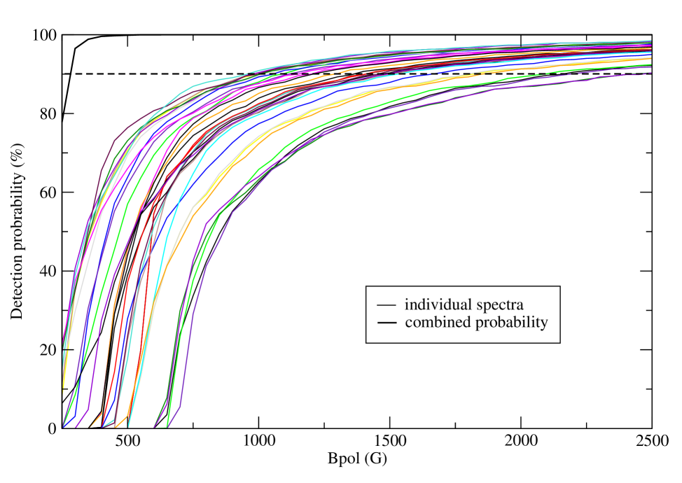
We required a 90% detection rate to consider that the field would statistically be detected. This translates into an upper limit for the possible undetected dipolar field strength for each spectrum, which varies between $\sim$900 and $\sim$2350 G (see Fig. 7).

Since 36 spectra are at our disposal, statistics can be combined to extract a stricter upper limit taking into account that the field has not been detected in any of the 36 observations (see Neiner et al. 2015). The final upper limit derived from this combined probability for $\zeta$ Ori Ab for a 90% detection probability is $\sim$300 G (see thick line in Fig. 7).

7 Magnetic field configuration

7.1 Rotational modulation

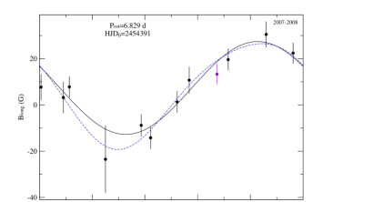
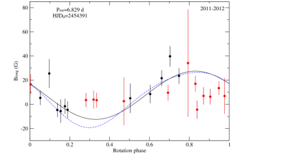
We searched for a period of variation in the 36 longitudinal magnetic field measurements of $\zeta$ Ori Aa with the clean-NG algorithm (see Gutiérrez-Soto et al. 2009). We obtained a frequency $f=0.146421$ c d^-1, which corresponds to a period of 6.829621 days. This value is consistent with the period of $\sim$7 days suggested by Bouret et al. (2008). Assuming that the magnetic field is a dipole with its axis inclined to the rotation axis, as is found in the vast majority of massive stars, this period corresponds to the rotation period of the star.

We used this period and plotted the longitudinal magnetic field as a function of phase. For the data taken in 2007 and 2008, the phase-folded field measurements show a clear sinusoidal behavior, as expected from a dipolar field model (see top panel of Fig. 8). A dipolar fit to the data, that is, a sine fit of the form $B(x)=B_{0}+B_{a}\times sin(2\pi(x+\phi_{d}))$, resulted in $B_{0}$=6.9 G and $B_{a}$=19.2 G. A quadrupolar fit to the phase-folded data only shows an insignificant departure from the dipolar fit.

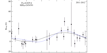
However, the period of $\sim$6.829 days does not to match the measurements collected in 2011 and 2012 very well (see middle panel of Fig. 8). None of the dipolar or quadrupolar fits to these data provide a reasonable match. A further search for a different period in these 2011-2012 data alone provided no significant result.

The magnetic fields of main-sequence massive stars are of fossil origin. These fields are known to be stable over decades and are only modulated by the rotation of the star. A change of period in the field modulation between the 2007-8 and 2011-12 epochs is thus not expected in $\zeta$ Ori Aa.

$\zeta$ Ori Aa has a companion, therefore we investigated the possibility that the magnetic field has been affected by the companion. Indeed, in 2011 and 2012, $\zeta$ Ori Ab was close to periastron, which means that the distance between the two stars was smaller than in 2007 and 2008. We calculated this distance to check whether some binary interactions might have occurred.

To calculate the distance between the two components, we used the photometric distance of $\zeta$ Ori A, d=387 pc (Hummel et al. 2013). From Hummel et al. (2013), we know the orbital parameters of the binary. The shortest distance between the two stars is $r_{\rm min}=a-\sqrt{a^{2}-b^{2}}$= 23.8 mas, where a is the semi-major axis and b the semi-minor axis. From the distance of $\zeta$ Ori A, we can compute $r_{\rm min}=\sin(\theta)/d$ in pc, where $\theta$ is the parallax in radian. We obtained a distance of 81 R_∗, where R_∗ is the radius of $\zeta$ Ori Aa.

The distance between the two stars at periastron therefore appears too large for interactions between the two stars to occur. In addition, the binary system is still significantly eccentric (0.338, Hummel et al. 2013) even though $\zeta$ Ori Aa has already evolved into a supergiant. Tidal interactions have apparently not been able to circularize the system yet, which would confirm that these interactions are weak (Zahn 2008).

However, in addition to $\zeta$ Ori Aa and Ab, a third star $\zeta$ Ori B may also interfere with the $\zeta$ Ori A system. Correia et al. (2012) showed that when a third component comes into play, tidal effects combined with gravitational interactions may increase the eccentricity of $\zeta$ Ori A, which would otherwise have circularized. We thus cannot exclude that tidal interactions are stronger than they seem in the $\zeta$ Ori A system.

Figure 8: Rotational modulation of the longitudinal magnetic field of $\zeta$ Ori Aa for the observations taken in 2007-2008 (top) and 2011-2012 (center). The black line corresponds to the best dipolar fit, while the dashed blue line corresponds to the best quadrupolar fit. The bottom panel compares the fit of the dipole and the quadrupole obtained from the 2007-2008 data with the observations obtained in 2011-2012 (see Sect. 7.3). The data for which the Stokes V model matches the observed LSD V profiles are shown in black, while the data for which the Stokes V model does not match are in red.

7.2 Field strength and geometrical configuration

Assuming that the period detected in Sect. 7.1 is the rotation period of the star, we can determine the inclination angle of the star $i$ by measuring $v\sin{i}$. In massive stars, line broadening does not come from rotational broadening alone, but also from turbulence and stellar wind. This is particularly true for supergiant stars.

Based on the synthetic spectra calculated in Sect. 4.1 and the lines identified to belong to only one of the two components, we determined the broadening needed in the synthetic spectra to fit the observations. For $\zeta$ Ori Aa, a broadening of 230 km s^-1 was necessary to provide a good fit to the observed lines, while for $\zeta$ Ori Ab we needed 100 km s^-1. These broadening values are upper limits of the $v\sin{i}$ values because they include all physical processes that broaden the lines. In fact, with a period of 6.829 days and a radius of 20 R_⊙ as given by Hummel et al. (2013), the maximum possible $v\sin{i}$ for $\zeta$ Ori Aa is 148 km s^-1.

In addition, Bouret et al. (2008) determined $v\sin{i}$ through a Fourier transform of the average of the 5801 and 5812 Å CIV and 5592 Å OIII line profiles. They found a $v\sin{i}$ of 110$\pm$10 km s^-1. From our disentangling of the spectra, we know that the two CIV lines originate from $\zeta$ Ori Aa, but the OIII 5590 Å line is partly ($\sim$10%) polluted by $\zeta$ Ori Ab. As a consequence, we applied the Fourier transform method to the LSD Stokes I profiles we calculated from the lines that only originate from $\zeta$ Ori Aa. We obtained $v\sin{i}$= 140 km s^-1. However, it is known that $v\sin{i}$ values determined from LSD profiles might be overestimated.

Finally, taking macroturbulence into account but not binarity, foe example, Simón-Díaz & Herrero (2014) found that $v\sin{i}$ for $\zeta$ Ori A is between 102 and 127 km s^-1, depending on the method they used.

In the following, we thus consider that $v\sin{i}$ is between 100 km s^-1and 148 km s^-1for $\zeta$ Ori Aa. In addition, we adopt the radius of 20 R_⊙ given by Hummel et al. (2013) and the rotation period of 6.829 d. Using $v\sin{i}$= [100-148] km s^-1, we obtain $i\sim[42-87]^{\circ}$.

Using the dipolar fit to the 2007-2008 longitudinal field measurements and the inclination angle $i$, we can deduce the obliquity angle $\beta$ of the magnetic field with respect to the rotation axis. To this aim, we used the formula $r=B_{\rm min}/B_{\rm max}=\cos(i-\beta)/\cos(i+\beta)$ (Shore 1987). The dipolar fit of the longitudinal field values gives $r$=0.47. With $i\sim[42-87]^{\circ}$, we obtain $\beta\sim[71-8]^{\circ}$.

In addition, from the dipolar fit to the longitudinal field values and the angles $i$ and $\beta$ determined above, we can estimate the polar field strength with the formula $B_{0}\pm B_{a}=0.296\times B_{\rm pol}\cos(\beta\pm i)$, where the limb-darkening coefficient is assumed to be 0.4 (see Borra & Landstreet 1980). We found $B_{\rm pol}$ = $[110\pm 5-524\pm 65]$ G. The dipolar magnetic field that we find is thus higher than the one found by Bouret et al. (2008).

In 2011-2012, the maximum measured B_l is 51 G and the minimum polar field strength is thus $B_{\rm pol}\geq 3.3B_{l,max}=168\pm 33$ G. This value is compatible with the range derived from the 2007-2008 data.

7.3 Stokes V modeling

Since the $B_{l}$ data taken in 2007-2008 point toward the presence of a dipole field, we used an oblique rotator model to fit the LSD Stokes V and I profiles.

We used Gaussian local intensity profiles with a width calculated according to the resolving power of Narval and a macroturbulence value of 100 km s^-1 determined by Bouret et al. (2008). We fit the observed LSD I profiles by Gaussian profiles to determine the depth, $v\sin{i}$  and radial velocity of the intensity profile. We used the weighted mean Landé factor and wavelength derived from the LSD mask applied to the Narval observations and the rotation period of 6.829 days. The fit includes five parameters: i, $\beta$, B_pol, a phase shift $\phi$, and a possible off-centering distance d_d of the dipole with respect to the center of the star (d_d=0 for a centered dipole and d_d=1 if the center of the dipole is at the surface of the star).

Figure 9: Best dipolar model fit (green) of the observed Stokes V profiles (black). The green numbers correspond to the rotational phase. The very noisy observation at phase 0.793 is not shown.

8 Magnetospheres

8.1 Magnetospheric parameters

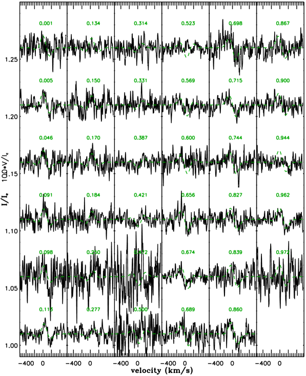
We calculated a grid of V profiles for each phase of observation by varying the five parameters mentioned above and applied a $\chi^{2}$ minimization to obtain the best fit of all observations simultaneously. More details of the modeling technique can be found in Alecian et al. (2008). The parameters of the best fit are i=79.89^∘, $\beta$=21.5^∘, $\phi$=0.68, B_pol=142.2 G and d_d=0.0. The values for the angles $i$ and $\beta$ are within the error boxes derived in Sect. 7.2, and the value for the polar field strength B_pol fits the $B_{l}$ results well. Moreover, the best fit is obtained for d_d=0, which confirms that no quadrupolar component is found.

The 36 Stokes V profiles for this best fit are shown in Fig. 9 overplotted on the observations. As expected, for the nights in 2007-2008, the model fits the observations well. For some nights in 2011-2012, the observations are too noisy to see whether the model fits well. Considering the nights in 2011-2012 for which the S/N is sufficient, the model fits some the observations but not all. For those nights for which the model fitted well the observations, we compared the values of the longitudinal magnetic field B_l to the dipolar fit obtained for the B_l measurements of 2007-2008 (see bottom panel of Fig. 8). The 2011-2012 data that match the Stokes V models also match the $B_{l}$ dipolar fit curve. Therefore, it seems that at least part of the 2011-2012 data show the same rotational modulation and dipole field as in 2007-2008. Only part of the 2011-2012 dataset does not match the rest of the observations.

With the polar magnetic field strength $B_{\rm pol}$ = 142.2 G determined with to the Stokes V model, we calculated the wind confinement parameter $\eta_{*}$ which characterizes the ability of the magnetic field to confine the wind particles into a magnetosphere (ud-Doula & Owocki 2002). If $\eta_{*}\leq 1$, $\zeta$ Ori Aa is located in the weakly magnetized winds region of the magnetic confinement-rotation diagram and it does not have a magnetosphere. However, for $\eta_{*}>1$, wind material is channeled along magnetic field lines toward the magnetic equator and $\zeta$ Ori Aa hosts a magnetosphere.

To calculate $\eta_{*}$, we first used the fiducial mass-loss rate $\dot{M}_{B=0}=1.4\times 10^{-6}M_{\odot}\leavevmode\nobreak\ yr^{-1}$ and the terminal speed V${}_{\infty}=2100$ km s^-1 determined by Bouret et al. (2008). They measured the mass-loss rate from the emission of H$\alpha$ and used archival International Ultraviolet Explorer (IUE) spectra to measure the wind terminal velocity from the blueward extension of the strong UV P Cygni profile. We obtain $\eta_{*}$ = 0.9.

We then recalculated $\eta_{*}$ but this time using the mass-loss rate of $\dot{M}=3.4\times 10^{-7}M_{\odot}\leavevmode\nobreak\ yr^{-1}$ and V${}_{\infty}=1850$ km s^-1 determined by Cohen et al. (2014). This gives $\eta_{*}$ = 4.2.

A magnetosphere can only exist below the Alfvén radius $R_{A}$, which is proportional to $\eta_{*}$, with $R_{A}=\eta_{*}^{1/4}R_{*}$. For $\zeta$ Ori Aa, using the two above determinations of $\eta_{*}$, $R_{A}=[0.98-1.43]R_{*}$. Moreover, the magnetosphere can be centrifugally supported above the corotation Kepler radius $R_{K}$. $R_{K}=(2\pi R_{*}/P_{\rm rot}\sqrt{(}GM/R_{*}))^{2/3}$, thus for $\zeta$ Ori Aa $R_{K}=2.8R_{*}$. Since $R_{K}$ ¿ $R_{A}$, no centrifugally supported magnetosphere can exist.

Therefore, $\zeta$ Ori Aa is either in the weakly magnetized winds region of the magnetic confinement-rotation diagram, meaning that $\zeta$ Ori Aa does not have a magnetosphere ($\eta_{*}<1$), or it hosts a dynamical magnetosphere ($1<\eta_{*}<4.2$).

8.2 H_α variations

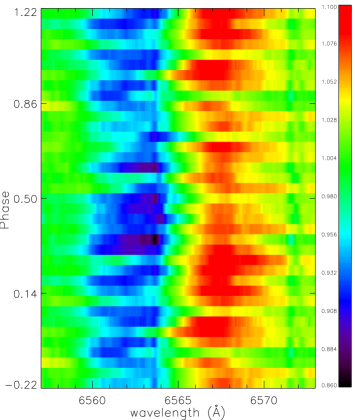
The H_α line shows significant variability in emission and absorption. For stars that have a magnetosphere, we expect magnetospheric emission at H_α, which varies with the rotation period (see e.g. Grunhut 2015).

To check whether there is a signature of the presence of a magnetosphere around $\zeta$ Ori Aa, we studied the variation of its H_α line in the archival spectra (see Sect. 2.2). We confirm that the emission in H_α does indeed vary. While most of the variations are problably related to variations in the stellar wind of the supergiant, the signature of a weak rotationally modulated dynamical magnetosphere is observed in H_α (see Fig. 10).

The ratio $\log R_{A}/R_{K}$ gives a measure of the volume of the magnetosphere. For $\zeta$ Ori Aa, $\log R_{A}/R_{K}$ is very small ($<$ 0.06), and it is thus not surprising that H_α only weakly reflects magnetic confinement.

Figure 10: Dynamic plot of each individual archival H_α spectrum in phase with the rotation period.

9 Discussion and conclusions

Based on archival spectrocopic data and Narval spectropolarimetric data, we confirm the presence of a magnetic field in the massive star $\zeta$ Ori A, as initally suggested by Bouret et al. (2008). However, Bouret et al. (2008) ignored that $\zeta$ Ori A is a binary star, which was subsequently shown by Hummel et al. (2013) with interferometry.

We disentangle the spectra and could thus show that the primary O supergiant component $\zeta$ Ori Aa is the magnetic star, while the secondary $\zeta$ Ori Ab is not magnetic at the achieved detection level. $\zeta$ Ori Aa is the only magnetic O supergiant known as of today.

The magnetic field of $\zeta$ Ori Aa is a typical oblique dipole field, similar to those observed in main-sequence massive stars. From Stokes modeling, the polar magnetic field strength $B_{\rm pol}$ of $\zeta$ Ori Aa is found to be about 140 G. If we assume field conservation during the evolution of $\zeta$ Ori Aa because the stellar radius increased from $\sim$10 to $\sim$20 R_⊙, the surface magnetic polar field strength decreased by a factor $\sim$4. This implies that the polar field strength of $\zeta$ Ori Aa when it was on the main sequence was about 600 G. This is similar to what is observed in other main-sequence magnetic O stars.

The current field strength and rotation rate of $\zeta$ Ori Aa are weak, with respect to the wind energy, for the star to be able to host a centrifugally supported magnetosphere. However, it seems to host a dynamical magnetosphere. All other ten known magnetic O stars host dynamical magnetospheres, except for the complicated system of Plaskett’s star, which has a very strong magnetic field and hosts a centrifugally supported magnetosphere (see Grunhut et al. 2013). However, these other magnetic O stars are not supergiants.

Although $\zeta$ Ori A is one of the brightest O star in the X-ray domain, Cohen et al. (2014) found that it resembles a non-magnetic star, with no evidence for magnetic activity in the X-ray domain and a spherical wind. This probably results from the weakness of the magnetosphere around $\zeta$ Ori Aa.

The rotation period of $\zeta$ Ori Aa, $P_{\rm rot}$ = 6.829 d, was determined from the variations of the longitudinal magnetic field. This period is clearly seen in the data obtained in 2007-2008, but only part of the spectropolarimetric measurements obtained in 2011 and 2012 seem to follow that rotational modulation. The reason for the lack of periodicity for part of the magnetic measurements of 2011-2012 was not identified. Although passage at the binary periastron occured between 2008 and 2011, the distance between the two companions seems too large for the companion to have perturbed the magnetic field of the primary star, unless it is $\zeta$ Ori B which has maintained the two components of $\zeta$ Ori A at a distance (see Sect. 7.1).

$\zeta$ Ori A therefore remains an interesting star that needs to be studied further. More spectropolarimetric observations should be collected at appropriate orbital phases to allow for a more accurate spectral disentangling. this would allow obtaining stronger constraints on the magnetic field strength and configuration, studying the field as a function of orbital phase, and understanding the magnetic field perturbations that seem to have occurred during the observations in 2011-2012.

Figure 11: LSD Stokes I profiles (bottom) computed from the disentangled spectroscopic data, Stokes V (top) and null N (middle) profiles, normalized to Ic, from the Narval data, for $\zeta$ Ori A. The red line is a smoothed profile.