Concordance maps in knot Floer homology

Abstract.

We show that a decorated knot concordance $\mathcal{C}$ from $K$ to $K^{\prime}$ induces a homomorphism $F_{\mathcal{C}}$ on knot Floer homology that preserves the Alexander and Maslov gradings. Furthermore, it induces a morphism of the spectral sequences to $\widehat{\mathit{HF}}(S^{3})\cong\mathbb{Z}_{2}$ that agrees with $F_{\mathcal{C}}$ on the $E^{1}$ page and is the identity on the $E^{\infty}$ page. It follows that $F_{\mathcal{C}}$ is non-vanishing on $\widehat{\mathit{HFK}}_{0}(K,\tau(K))$. We also obtain an invariant of slice disks in homology 4-balls bounding $S^{3}$.

If $\mathcal{C}$ is invertible, then $F_{\mathcal{C}}$ is injective, hence

$$\dim\widehat{\mathit{HFK}}_{j}(K,i)\leq\dim\widehat{\mathit{HFK}}_{j}(K^{\prime},i)$$

for every $i$, $j\in\mathbb{Z}$. This implies an unpublished result of Ruberman that if there is an invertible concordance from the knot $K$ to $K^{\prime}$, then $g(K)\leq g(K^{\prime})$, where $g$ denotes the Seifert genus. Furthermore, if $g(K)=g(K^{\prime})$ and $K^{\prime}$ is fibred, then so is $K$.

1. Introduction

Knot Floer homology was introduced independently by Ozsváth-Szabó [29] and Rasmussen [32], and the first author [16] defined maps induced on it by decorated knot cobordisms. Given a knot $K$ in $S^{3}$, its knot Floer homology with $\mathbb{Z}_{2}$ coefficients is a finite dimensional bigraded $\mathbb{Z}_{2}$ vector space

$$\bigoplus_{i,j\in\mathbb{Z}}\widehat{\mathit{HFK}}_{j}(K,i),$$

well-defined up to isomorphism, where $i$ is called the Alexander grading and $j$ is the homological grading. The Euler characteristic of $\widehat{\mathit{HFK}}_{*}(K,i)$ is the $i$-th coefficient of the symmetrized Alexander polynomial of $K$, and hence knot Floer homology can be viewed as a categorification of the Alexander polynomial. First, we recall [16, Definition 4.1].

Definition 1.1.

For $i\in\{0,1\}$, let $Y_{i}$ be a connected, oriented 3-manifold, and let  $L_{i}$ be a non-empty link in $Y_{i}$. Then a link cobordism from $(Y_{0},L_{0})$ to $(Y_{1},L_{1})$ is a pair $(X,F)$, where

1. $X$ is a connected, oriented cobordism from $Y_{0}$ to $Y_{1}$,

2. $F$ is a properly embedded, compact, orientable surface in $X$, and

3. $\partial F=L_{0}\cup L_{1}$.

Knots $K_{0}$ and $K_{1}$ in $S^{3}$ are said to be concordant if there is a cobordism $(X,F)$ from $(S^{3},K_{0})$ to $(S^{3},K_{1})$ such that $X=S^{3}\times I$ and $F$ is diffeomorphic to $S^{1}\times I$. In this case, we call $(X,F)$ a concordance from $K_{0}$ to $K_{1}$. In this paper, we also allow more general concordances where $X$ is a cobordism from $S^{3}$ to $S^{3}$ such that $H_{1}(X)=H_{2}(X)=0$.

In this paper, a decorated knot is a pair $(K,P)$ such that $K$ is a knot, $P$ is a pair of points in $K$, and we are given a decomposition of $K$ into compact $1$-manifolds $R_{+}(P)$ and $R_{-}(P)$ such that $R_{+}(P)\cap R_{-}(P)=P$. Given decorated knots $(K_{0},P_{0})$ and $(K_{1},P_{1})$ in $S^{3}$, a decorated concordance from $(K_{0},P_{0})$ to $(K_{1},P_{1})$ is a triple $(X,F,\sigma)$ such that $(X,F)$ is a concordance from $K_{0}$ to $K_{1}$, and $\sigma$ consists of two disjoint, properly embedded arcs in $F$, one connecting $R_{+}(K_{0})$ and $R_{+}(K_{1})$, the other $R_{-}(K_{0})$ and $R_{-}(K_{1})$.

Dylan Thurston and the first author [17] showed that knot Floer homology is natural for decorated knots, and Sarkar [36] proved that moving the basepoints $P$ around the knot induces a non-trivial automorphism in many cases. Hence only decorated concordances induce maps on knot Floer homology.

Recall that [29, Lemma 3.6], for every decorated knot $(K,P)$ in $S^{3}$, there is a corresponding spectral sequence

$$\widehat{\mathit{HFK}}(K,P)\Rightarrow\widehat{\mathit{HF}}(S^{3})\cong\mathbb{Z}_{2}.$$

Given an admissible doubly-pointed Heegaard diagram $(\Sigma,\boldsymbol{\alpha},\boldsymbol{\beta},w,z)$ for $(K,P)$, the singly-pointed diagram $(\Sigma,\boldsymbol{\alpha},\boldsymbol{\beta},w)$ represents $(S^{3},w)$, and $z$ gives rise to the knot filtration on $\widehat{\mathit{CF}}(\Sigma,\boldsymbol{\alpha},\boldsymbol{\beta},w)$. The spectral sequence arises from this filtered complex. The $E^{0}$ page is the associated graded complex $\widehat{\mathit{CFK}}(\Sigma,\boldsymbol{\alpha},\boldsymbol{\beta},w,z)$, whose homology is $\widehat{\mathit{HFK}}(K,P)$, the $E^{1}$ page. The spectral sequence limits to the homology of $\widehat{\mathit{CF}}(\Sigma,\boldsymbol{\alpha},\boldsymbol{\beta},w)$, which is $\widehat{\mathit{HF}}(S^{3})\cong\mathbb{Z}_{2}$. The filtration level of the generator of $\mathbb{Z}_{2}$ in the $E^{\infty}$ page is the Ozsváth-Szabó $\tau$ invariant [27], denoted by $\tau(K)$.

The main result of this paper is that a decorated concordance $\mathcal{C}$ induces a non-vanishing homomorphism $F_{\mathcal{C}}$ on knot Floer homology that preserves the Alexander and homological gradings, and also induces a morphism of the corresponding spectral sequences. The map $F_{\mathcal{C}}$ is functorial and depends only on the decorated concordance $\mathcal{C}$, while the chain map $f_{\mathcal{C}}$ (or even its filtered homotopy type) need not be functorial, and it can depend on auxiliary data other than $\mathcal{C}$.

Theorem 1.2.

Let $(K_{0},P_{0})$ and $(K_{1},P_{1})$ be decorated knots in $S^{3}$, and let $\mathcal{C}=(X,F,\sigma)$ be a decorated concordance between them such that $H_{1}(X)=H_{2}(X)=0$. Then

$$F_{\mathcal{C}}\left(\widehat{\mathit{HFK}}_{j}(K_{0},P_{0},i)\right)\leq\widehat{\mathit{HFK}}_{j}(K_{1},P_{1},i)$$

for every $i$, $j\in\mathbb{Z}$.

Furthermore, given an admissible diagram $(\Sigma_{r},\boldsymbol{\alpha}_{r},\boldsymbol{\beta}_{r},w_{r},z_{r})$ of $(K_{r},P_{r})$ for $r\in\{0,1\}$, there is a filtered chain map

$$f_{\mathcal{C}}\colon\widehat{\mathit{CF}}(\Sigma_{0},\boldsymbol{\alpha}_{0},\boldsymbol{\beta}_{0},w_{0})\to\widehat{\mathit{CF}}(\Sigma_{1},\boldsymbol{\alpha}_{1},\boldsymbol{\beta}_{1},w_{1})$$

of homological degree zero such that the induced morphism of spectral sequences agrees with $F_{\mathcal{C}}$ on the $E^{1}$ page and with $\text{Id}_{\mathbb{Z}_{2}}$ on the total homology and on the $E^{\infty}$ page.

Note that the fact that the map induced by a filtered map $f$ on the total homology is an isomorphism in general does not imply that the map $f^{\infty}$ induced between the $E^{\infty}$ pages is also an isomorphism. As an example, consider a complex $C\cong\mathbb{Z}_{2}$ in filtration level one, and a complex $\overline{C}\cong\mathbb{Z}_{2}$ in filtration level zero. If $f\colon C\to\overline{C}$ is an isomorphism, then $H(f)$ is an isomorphism but $f^{\infty}$ is not.

In the case of the filtered map $f_{\mathcal{C}}$ induced by a decorated concordance $\mathcal{C}$, the fact that $f_{\mathcal{C}}^{\infty}$ is an isomorphism follows from the fact that $\tau(K_{0})=\tau(K_{1})$, which was shown by Ozsváth and Szabó [27, Theorem 1.1]. An alternative proof of this can be given by observing that a decorated concordance gives filtered maps both ways that induce isomorphisms on the total homology, as in the proofs of [33, Theorem 1] and [35, Theorem 3.4].

The invariant $\tau(K)$ can also be defined as the smallest Alexander grading of an element of $\widehat{\mathit{HFK}}(K,P)$ that represents a cycle on each page of the spectral sequence, and whose homology class in the $E^{\infty}$ page is $1$. We denote the set of such elements by $A_{1}(K)$. Then we have the following non-vanishing result for the knot concordance maps:

Corollary 1.3.

Let $(K_{0},P_{0})$ and $(K_{1},P_{1})$ be decorated knots in $S^{3}$, and suppose that $\mathcal{C}=(X,F,\sigma)$ is a decorated concordance between them. Let $\tau=\tau(K_{0})=\tau(K_{1})$. Then, the map

$$F_{\mathcal{C}}\colon\widehat{\mathit{HFK}}_{0}(K_{0},P_{0},\tau)\to\widehat{\mathit{HFK}}_{0}(K_{1},P_{1},\tau)$$

is non-zero, and $F_{\mathcal{C}}(A_{1}(K_{0}))\subseteq A_{1}(K_{1})$.

In fact, for any decorated knot $(K,P)$ in $S^{3}$, we shall see that

$$A_{1}^{\prime}(K):=A_{1}(K)\cap\widehat{\mathit{HFK}}_{0}(K,P,\tau(K))\neq\emptyset,$$

and the map $F_{\mathcal{C}}\colon A_{1}^{\prime}(K_{0})\to A_{1}^{\prime}(K_{1})$ is non-zero.

Let $B$ be an integral homology 4-ball with boundary $S^{3}$. Suppose that $S\subset B$ is a slice disk for the decorated knot $(K,P)$ in $S^{3}$. If we remove a ball from $B$ about a point of $S$, we obtain a concordance $\mathcal{C}(S)$ from the unknot $U$ to $K$. By Lemma 3.11, the element

$$t_{S,P}:=F_{\mathcal{C}(S)}(1)\in\widehat{\mathit{HFK}}_{0}(K,P,0)$$

is independent of what decoration we choose on $\mathcal{C}(S)$. It is non-zero by Corollary 1.3, and is an invariant of the surface $S$ up to isotopy in $B$ fixing $K$.

Question 1.4.

Can $t_{S,P}$ distinguish different slice disks? More precisely, is there a decorated knot $(K,P)$ in $S^{3}$ that has two different slice disks $S$ and $S^{\prime}$ in $D^{4}$ such that $t_{S,P}\neq t_{S^{\prime},P}$?

Note that, given different decorations $P$ and $P^{\prime}$ on $K$, the basepoint moving map of Sarkar [36] takes $t_{S,P}$ to $t_{S,P^{\prime}}$, so the answer is independent of the choice of basepoints.

We can use the above viewpoint to refine the approach of Freedman, Gompf, Morrison, and Walker [6] for disproving the smooth 4-dimensional Poincaré conjecture (SPC4). Suppose that we are given a counterexample to SPC4 with no 3-handles and a single 4-handle. Removing the 4-handle, we obtain an exotic 4-ball $B$ with boundary homeomorphic to $S^{3}$. The belt circles of the 2-handles give a link $L\subset\partial B$, and the cocores of the 2-handles give a collection of disks $C\subset B$ with boundary $L$. If we band sum the components of $L$ in some way, we obtain a knot $K\subset\partial B$, together with a disk $D\subset B$ obtained from $C$. Hence $D$ induces an element $t_{D,P}\in\widehat{\mathit{HFK}}(K,P)$ for any decoration $P$. If $t_{D,P}\neq t_{S,P}$ for $S$ an arbitrary slice disk of $K$, then this implies that $B$ is indeed exotic.

The approach of Freedman et al. only works if $K$ is not slice in the standard 4-ball, but it is in the homotopy 4-ball $B$. By the work of Ozsváth and Szabó [27, Theorem 1.1], the $\tau$-invariant vanishes if $K$ bounds a disk in a homotopy ball, and so does Rasmussen’s $s$-invariant according to Kronheimer and Mrowka [19], so neither can be used for the above purpose. We could use any other theory equipped with knot concordance maps in manifolds homeomorphic to $S^{3}\times I$. However, note that the Khovanov homology concordance maps of Jacobsson [12] are only defined when the ambient manifold is diffeomorphic to $S^{3}\times I$.

A knot is called doubly slice if it is a hyperplane cross-section of an unknotted $S^{2}$ in $S^{4}$. Motivated by a question of Fox [5] asking which knots are doubly slice, Sumners [39] introduced the notion of invertible knot cobordisms. In his terminology, cobordism stands for concordance; we use the latter for clarity.

Definition 1.5.

Let $K_{0}$ and $K_{1}$ be knots in $S^{3}$. We say that a concordance $(S^{3}\times I,F)$ from $K_{0}$ to $K_{1}$ is invertible if there is a concordance $(S^{3}\times I,F^{\prime})$ from $K_{1}$ to $K_{0}$ such that the composition of $(S^{3}\times I,F)$ and $(S^{3}\times I,F^{\prime})$ from $K_{0}$ to $K_{0}$ is equivalent to the trivial cobordism. We write $K_{0}\leq K_{1}$ if there is an invertible cobordism from $K_{0}$ to $K_{1}$.

In other words, $F$ is invertible if and only if $(S^{3}\times I,F)$ has a left inverse in the cobordism category of links. A knot $K$ is doubly slice if and only if $U\leq K$. The relation $\leq$ is a partial order on the set of knots in $S^{3}$, which follows from [37], as we shall explain later.

Theorem 1.6.

If there is an invertible concordance from $K_{0}$ to $K_{1}$, then

$$\dim\widehat{\mathit{HFK}}_{j}(K_{0},i)\leq\dim\widehat{\mathit{HFK}}_{j}(K_{1},i)$$

for every $i$, $j\in\mathbb{Z}$.

This provides an obstruction to the existence of an invertible concordance from $K_{0}$ to $K_{1}$. According to the work of Manolescu, Ozsváth, and Sarkar [23], knot Floer homology is algorithmically computable, and Baldwin and Gillam [3] used this algorithm to compute it for knots with at most 12 crossings.

For a knot $K$ in $S^{3}$, we denote its Seifert genus by $g(K)$. Ozsváth and Szabó [28] proved that knot Floer homology detects the genus of a knot, in the sense that

$$g(K)=\max\{\,i\in\mathbb{Z}\,\colon\,\widehat{\mathit{HFK}}_{*}(K,i)\neq 0\,\}.$$

For a simpler proof of this fact, see [25]. Furthermore, knot Floer homology also detects fibredness of knots, as $\dim\widehat{\mathit{HFK}}_{*}(K,g(K))=1$ if and only if $K$ is fibred. This was shown by Ghiggini [8] in the genus one case, and by Ni [25, 26] and the first author [14, 15] in the general case. These two results, together with Theorem 1.6, immediately imply the following unpublished result of Ruberman.

Corollary 1.7.

The function $g$ is monotonic with respect to the partial order $\leq$ induced by invertible concordance. More concretely, if there is an invertible concordance from $K_{0}$ to $K_{1}$, then $g(K_{0})\leq g(K_{1})$. Furthermore, if $K_{1}$ is fibred and $g(K_{0})=g(K_{1})$, then $K_{0}$ is also fibred.

We now outline a more elementary proof of these results communicated to us by Ruberman, and which does not use the assumption $g(K_{0})=g(K_{1})$ for the second statement. Also see the proof of [37, Proposition 3.7] and the paragraph following it.

Proof.

Let $F$ be an invertible concordance from $K_{0}$ to $K_{1}$ with inverse $F^{\prime}$. Then there is a diffeomorphism $d\colon S^{3}\times I\to S^{3}\times I$ such that $d(F^{\prime}\circ F)=K_{0}\times I$ and $d|_{S^{3}\times\partial I}$ is the identity. Let $i\colon S^{3}\to S^{3}\times I$ be the embedding $i(x)=(x,1/2)$, and let $p\colon S^{3}\times I\to S^{3}$ be the projection. Then the composition

$$f=p\circ d\circ i\colon S^{3}\to S^{3}$$

maps $K_{1}$ to $K_{0}$ such that $f^{-1}(K_{0})=K_{1}$. We can isotope $d$ such that $d(K_{1}\times\{1/2\})$ becomes transverse to the $I$-fibration of $K_{0}\times I$, and hence $f|_{K_{1}}$ is an embedding with image $K_{0}$. If $S$ is a minimal genus Seifert surface for $K_{1}$, then $f|_{S}$ satisfies the conditions of [7, Corollary 6.23], hence there exists a Seifert surface $T$ of $K_{0}=f(K_{1})$ such that $g(T)\leq g(S)$. It follows that $g(K_{0})\leq g(K_{1})$. Recall that [7, Corollary 6.23] is a deep generalization of Dehn’s lemma to higher genus surfaces due to Gabai. It states that if $M$ is a compact oriented 3-manifold, $S$ a compact oriented surface with connected boundary, and $f\colon S\to M$ a map such that $f|_{\partial S}$ is an embedding and $f^{-1}(f(\partial S))=\partial S$, then there exists an embedded surface $T$ in $M$ such that $\partial T=f(\partial S)$ and $g(T)\leq g(S)$.

Let $E(K_{i})$ denote the exterior of the knot $K_{i}$ for $i\in\{0,1\}$. Then

$$f|_{E(K_{1})}\colon E(K_{1})\to E(K_{0})$$

is a degree one map as it is an orientation preserving diffeomorphism between the boundary tori. Hence, by [34, Lemma 1.2], it induces a surjection on the fundamental groups, and also on the commutator subgroups. If $K_{1}$ is fibred, then the commutator subgroup $\pi_{1}(E(K_{1}))^{\prime}$ is finitely generated, hence $\pi_{1}(E(K_{0}))^{\prime}$ is also finitely generated, so $K_{0}$ is fibred by a result of Stallings [38]. ∎

Let $K$ and $K^{\prime}$ be knots in $S^{3}$ such that there is an epimorphism $\pi_{1}(E(K))\to\pi_{1}(E(K^{\prime}))$ preserving peripheral structure. By [37], this induces a partial order $\succeq$ on the set of knots. For example, if there is a degree one map

$$(E(K),\partial E(K))\to(E(K^{\prime}),\partial E(K^{\prime})),$$

in particular if $K\geq K^{\prime}$, then $K\succeq K^{\prime}$. Notice that this implies that $\geq$ is also a partial order. Based on the above proof and Theorem 1.6, it is natural to ask whether $K\succeq K^{\prime}$ also implies that

(1.1) $$\dim\widehat{\mathit{HFK}}_{*}(K,i)\geq\dim\widehat{\mathit{HFK}}_{*}(K^{\prime},i)$$

for every $i\in\mathbb{Z}$. Note that this would imply [37, Conjecture 3.6] claiming that, if $K\succeq K^{\prime}$, then $g(K)\geq g(K^{\prime})$. Compare this with [18, Conjecture 9.4], which claims that if $f\colon Y\to Y^{\prime}$ is a non-zero degree map between integer homology spheres, then $\dim\widehat{\mathit{HF}}(Y)\geq\dim\widehat{\mathit{HF}}(Y^{\prime})$. However, inequality (1.1) turns out to be false due to the following example constructed by Jennifer Hom.

Example 1.8.

Let $K=(T_{2,3})_{2,3}$ be the $(2,3)$-cable of the right-handed trefoil $T_{2,3}$, and let $K^{\prime}=T_{2,3}$. Then $K\succeq K^{\prime}$. In fact, there is a degree one map

$$(E(K),\partial E(K))\to(E(K^{\prime}),\partial E(K^{\prime})).$$

Indeed, let $T\subset E(K)$ be the boundary of the solid torus used in the satellite construction for $K$. Then the exterior of $T$ is $E(K^{\prime})$, hence fibred over $S^{1}$. If we collapse the fibers to disks, we obtain a degree one map from the exterior of $T$ to $D^{2}\times S^{1}$, and hence from $E(K)$ to $E(K^{\prime})$. But both $K$ and $K^{\prime}$ are determined by their Alexander polynomials, $K^{\prime}$ because it is alternating, and $K$ by the work of Hedden [9, Theorem 1.0.6]. The symmetrized Alexander polynomial of $K$ is

$$t^{3}-t^{2}+1-t^{-2}+t^{-3},$$

while the symmetrized Alexander polynomial of $K^{\prime}$ is $t-1+t^{-1}$. So $\widehat{\mathit{HFK}}(K,1)=0$ and $\widehat{\mathit{HFK}}(K^{\prime},1)=\mathbb{Z}_{2}$, violating inequality (1.1).

In light of this, we propose the following weaker question.

Question 1.9.

Suppose that $K\succeq K^{\prime}$. Then is it true that

$$\dim\widehat{\mathit{HFK}}(K)\geq\dim\widehat{\mathit{HFK}}(K^{\prime})?$$

The paper is organized as follows. In Section 2, we review sutured manifold cobordisms and the maps induced by them on sutured Floer homology. In Section 3, we define the knot concordance maps, show that they preserve the Alexander grading (Proposition 3.10), and prove Theorem 1.6. Section 4 gives a brief overview of spectral sequences arising from a filtered complex. In Section 5, we show that, on the chain level, a knot concordance map can be represented by a chain map that preserves the Alexander filtration (Theorem 5.4) and therefore induces a morphism of spectral sequences (Theorem 5.5); this is precisely the second part of Theorem 1.2. Corollary 1.3 follows from Corollary 5.7. Finally, we prove in Section 6 that the knot concordance maps preserve the homological grading, which concludes the proof of Theorem 1.2.

Acknowledgement

We would like to thank Daniel Ruberman for pointing out a more elementary proof of Corollary 1.7, and Ciprian Manolescu for drawing our attention to the grading shift formula in [22] and for his comments on an earlier version of this paper. We are also grateful to Jennifer Hom for Example 1.8. Finally, we would like to thank the referee for the invaluable suggestions.

2. Cobordisms of sutured manifolds

In this section, we briefly review sutured manifold cobordisms, and the maps they induce on sutured Floer homology, as defined by the first author [16].

2.1. Sutured manifolds and sutured cobordisms

Definition 2.1 ([7, Definition 2.6]).

A sutured manifold is a compact oriented $3$-manifold $M$ with boundary together with a set $\gamma\subseteq\partial M$ of pairwise disjoint annuli $A(\gamma)$ and tori $T(\gamma)$. Furthermore, the interior of each component of $A(\gamma)$ contains a homologically non-trivial oriented simple closed curve, called a suture. We denote the set of sutures by $s(\gamma)$.

Finally, every component of $R(\gamma)=\partial M\setminus\text{Int}(\gamma)$ is oriented such that $\partial R(\gamma)$ is coherent with the sutures. Let $R_{+}(\gamma)$ (or $R_{-}(\gamma)$) denote the components of $R(\gamma)$ whose normal vectors points out of (into) $M$.

Definition 2.2 ([13, Definition 2.2]).

We say that a sutured manifold $(M,\gamma)$ is balanced if $M$ has no closed components, $\chi(R_{+}(\gamma))=\chi(R_{-}(\gamma))$, and the map $\pi_{0}(A(\gamma))\to\pi_{0}(\partial M)$ is surjective.

From now on, we only consider sutured manifolds where $T(\gamma)=\emptyset$, and view $\gamma$ as a “thickened” oriented 1-manifold. So we often do not distinguish between $\gamma$ and $s(\gamma)$; it shall be clear from the context which one we mean.

Definition 2.3 ([16, Definition 2.3]).

Let $(M,\gamma)$ be a sutured manifold, and suppose that $\xi_{0}$ and $\xi_{1}$ are contact structures on $M$ such that $\partial M$ is a convex surface with dividing set $\gamma$ with respect to both $\xi_{0}$ and $\xi_{1}$. Then we say that $\xi_{0}$ and $\xi_{1}$ are equivalent if there is a 1-parameter family $\left\{\xi_{t}\,\colon\,t\in I\right\}$ of contact structures such that $\partial M$ is convex with dividing set $\gamma$ with respect to $\xi_{t}$ for every $t\in I$. In this case, we write $\xi_{0}\sim\xi_{1}$, and we denote by $[\xi]$ the equivalence class of the contact structure $\xi$.

Definition 2.4 ([16, Definitions 2.4 and 2.14]).

Let $(M_{0},\gamma_{0})$ and $(M_{1},\gamma_{1})$ be sutured manifolds. A cobordism from $(M_{0},\gamma_{0})$ to $(M_{1},\gamma_{1})$ is a triple $\mathcal{W}=(W,Z,[\xi])$, where

• $W$ is a compact oriented $4$-manifold with boundary,

• $Z\subseteq\partial W$ is a compact, codimension-$0$ submanifold with boundary (viewed within $\partial W$), such that $\partial W\setminus\text{Int}(Z)=-M_{0}\sqcup M_{1}$, and we view $Z$ as a sutured manifold with sutures $\gamma_{0}\cup\gamma_{1}$,

• $\xi$ is a positive contact structure on $Z$ such that $\partial Z$ is a convex surface with dividing set $\gamma_{i}$ on $\partial M_{i}$ for $i\in\{0,1\}$.

Finally, a cobordism is called balanced if both $(M_{0},\gamma_{0})$ and $(M_{1},\gamma_{1})$ are balanced.

In this paper, we will only consider balanced sutured manifolds and balanced cobordisms.

Definition 2.5 ([16, Definition 2.7]).

Two cobordisms $\mathcal{W}=(W,Z,[\xi])$ and $\mathcal{W}^{\prime}=(W^{\prime},Z^{\prime},[\xi^{\prime}])$ from $(M_{0},\gamma_{0})$ to $(M_{1},\gamma_{1})$ are called equivalent if there is an orientation preserving diffeomorphism $\varphi:W\to W^{\prime}$ such that $d(Z)=Z^{\prime}$, $d_{*}(\xi)=\xi^{\prime}$, and $d|_{M_{0}\cup M_{1}}=\text{Id}$.

Definition 2.6 ([16, Definition 10.4]).

A cobordism $\mathcal{W}=(W,Z,[\xi])$ from $(M_{0},\gamma_{0})$ to $(N,\gamma_{1})$ is called a boundary cobordism if $W$ is balanced, $N$ is parallel to $M_{0}\cup(-Z)$, and we are also given a deformation retraction $r:W\times\left[0,1\right]\longrightarrow M_{0}\cup(-Z)$ such that $r_{0}|_{W}=\text{Id}_{W}$ and $r_{1}|_{N}$ is an orientation preserving diffeomorphism from $N$ to $M_{0}\cup(-Z)$.

Definition 2.7 ([16, Definition 5.1]).

We say that a cobordism $\mathcal{W}=(W,Z,[\xi])$ from $(M_{0},\gamma_{0})$ to $(M_{1},\gamma_{1})$ is special if

1. $\mathcal{W}$ is balanced;

2. $\partial M_{0}=\partial M_{1}$, and $Z=\partial M_{0}\times I$ is the trivial cobordism between them;

3. $\xi$ is an $I$-invariant contact structure on $Z$ such that each $\partial M_{0}\times\left\{t\right\}$ is a convex surface with dividing set $\gamma_{0}\times\left\{t\right\}$ for every $t\in I$ with respect to the contact vector field $\partial/\partial t$.

In particular, it follows from (3) that $\gamma_{0}=\gamma_{1}$.

Remark 2.8.

Every sutured cobordism can be seen as the composition of a boundary cobordism and a special cobordism, cf. [16, Definition 10.1]. Let $\mathcal{W}=(W,Z,[\xi])$ be a balanced cobordism from $(M_{0},\gamma_{0})$ to $(M_{1},\gamma_{1})$. Let $(N,\gamma_{1})$ be the sutured manifold $(M_{0}\cup(-Z),\gamma_{1})$. Then we can think of the cobordism $\mathcal{W}$ as a composition $\mathcal{W}^{s}\circ\mathcal{W}^{b}$, where $\mathcal{W}^{b}$ is a boundary cobordism from $(M_{0},\gamma_{0})$ to $(N,\gamma_{1})$ and $\mathcal{W}^{s}$ is a special cobordism from $(N,\gamma_{1})$ to $(M_{1},\gamma_{1})$.

2.2. Relative $\text{Spin}^{c}$ structures

Definition 2.9 ([16, Definition 3.1]).

Given a sutured manifold $(M,\gamma)$, we say that a vector field $v$ defined on a subset of $M$ containing $\partial M$ is admissible if it is nowhere vanishing, it points into $M$ along $R_{-}(\gamma)$, it points out of $M$ along $R_{+}(\gamma)$, and $v|_{\gamma}$ is tangent to $\partial M$ and either points into $R_{+}(\gamma)$ or is positively tangent to $\gamma$ (we think of $\partial M$ as a smooth surface, and of $\gamma$ as a 1-manifold).

Let $v$ and $w$ be admissible vector fields on $M$. We say that $v$ and $w$ are homologous, and we write $v\sim w$, if there is a collection of balls $B\subseteq M$, one in each component of $M$, such that $v$ and $w$ are homotopic on $M\setminus B$ through admissible vector fields. Then $\text{Spin}^{c}(M,\gamma)$ is the set of homology classes of admissible vector fields on $M$.

If $(M,\gamma)$ is balanced, $\text{Spin}^{c}(M,\gamma)$ is an affine space over $H^{2}(M,\partial M)$. Throughout this paper, we will denote relative $\text{Spin}^{c}$ structures by $\mathfrak{s}^{\circ}$, to distinguish them from ordinary $\text{Spin}^{c}$ structures on oriented $3$-manifolds, usually denoted by $\mathfrak{s}$.

Remark 2.10.

Let $v_{0}$ be a fixed vector field on $\partial M$ arising as $v|_{\partial M}$ for some admissible vector field $v$ on $M$. We define $\text{Spin}^{c}_{v_{0}}(M,\gamma)$ as the set of nowhere vanishing vector fields on $M$ that restrict to $v_{0}$ on $\partial M$, up to isotopy through such vector fields relative to $\partial M$ in the complement of a collection of balls. Since the space of all possible $v_{0}$ is contractible, $\text{Spin}^{c}_{v_{0}}(M,\gamma)$ can be canonically identified with $\text{Spin}^{c}(M,\gamma)$. This was the approach taken in [13].

Definition 2.11 ([16, Definition 3.2]).

Let $(M,\gamma)$ be a sutured manifold. We say that an oriented 2-plane field $\xi$ defined on a subset of $M$ containing $\partial M$ is admissible if there exists a Riemannian metric $g$ on $M$ such that $\xi^{\perp_{g}}$ is an admissible vector field. If $\xi$ is defined on the whole manifold $M$, we write

$$\mathfrak{s}^{\circ}_{\xi}=[\xi^{\perp_{g}}]\in\text{Spin}^{c}(M,\gamma).$$

This is independent of the choice of $g$ since the space of metrics $g$ for which $\xi^{\perp_{g}}$ is an admissible vector field is convex.

We now recall the notion of relative $\text{Spin}^{c}$ structures on sutured cobordisms. If $J$ is an almost complex structure on a 4-manifold $W$ and $H$ is a 3-dimensional submanifold, then there is a 2-plane field induced on $H$ called the field of complex tangencies along $H$, cf. [16, Lemma 3.4].

Definition 2.12 ([16, Definition 3.5]).

Suppose that $\mathcal{W}=(W,Z,[\xi])$ is a cobordism from the sutured manifold $(M_{0},\gamma_{0})$ to $(M_{1},\gamma_{1})$. We say that an almost complex structure $J$ defined on a subset of $W$ containing $\partial Z$ is admissible if the field of complex tangencies on $M_{i}$ (defined on a subset of $M_{i}$ containing $\partial M_{i}$) is admissible in $(M_{i},\gamma_{i})$ for $i\in\left\{0,1\right\}$, and the field $\xi_{J}$ of complex tangencies on $Z$ (defined on a subset of $Z$ containing $\partial Z$) is admissible in $(Z,\gamma_{0}\cup\gamma_{1})$.

A relative $\text{Spin}^{c}$ structure on $\mathcal{W}$ is a homology class of pairs $(J,P)$, where:

• $P\subseteq\text{Int}(W)$ is a finite collection of points,

• $J$ is an admissible almost complex structure defined over $W\setminus P$,

• if $\xi_{J}$ is the field of complex tangencies along $Z$, then $\mathfrak{s}^{\circ}_{\xi}=\mathfrak{s}^{\circ}_{\xi_{J}}$.

We say that $(J,P)$ and $(J^{\prime},P^{\prime})$ are homologous if there exists a compact 1-manifold $C\subseteq W\setminus\partial Z$ such that $P$, $P^{\prime}\subseteq C$; furthermore, $J|_{W\setminus C}$ and $J^{\prime}|_{W\setminus C}$ are isotopic through admissible almost complex structures. We denote by $\text{Spin}^{c}(\mathcal{W})$ the set of relative $\text{Spin}^{c}$ structures over $\mathcal{W}$.

Remark 2.13.

As in the case of sutured manifolds, we will denote relative $\text{Spin}^{c}$ structures on sutured cobordisms by $\mathfrak{s}^{\circ}$, in order to distinguish them from ordinary $\text{Spin}^{c}$ structures on oriented 4-manifolds, which we denote by $\mathfrak{s}$, in analogy with the case of oriented 3-manifolds.

Remark 2.14.

$\text{Spin}^{c}(\mathcal{W})$ is an affine space over

$$\ker\left(H^{2}(W,\partial Z)\longrightarrow H^{2}(Z,\partial Z)\right).$$

There are restriction maps

$$\text{Spin}^{c}(W)\longrightarrow\text{Spin}^{c}(M_{i},\gamma_{i})$$

for $i\in\{0,1\}$.

2.3. Sutured Floer homology

The first author [13] associated an $\mathbb{F}_{2}$-vector space $\mathit{SFH}(M,\gamma)$ to each balanced sutured manifold $(M,\gamma)$, called the sutured Floer homology of $(M,\gamma)$. It splits along the relative $\text{Spin}^{c}$ structures on $(M,\gamma)$:

$$\mathit{SFH}(M,\gamma)=\bigoplus_{\mathfrak{s}^{\circ}\,\in\,\text{Spin}^{c}(M,\gamma)}\mathit{SFH}(M,\gamma,\mathfrak{s}^{\circ}).$$

Each vector space $\mathit{SFH}(M,\gamma,\mathfrak{s}^{\circ})$ is an invariant of the sutured manifold together with the relative $\text{Spin}^{c}$ structure. Sutured Floer homology is a common generalisation of Heegaard Floer homology of closed oriented 3-manifolds [30] and knot Floer homology [29, 32].

The first author proved [16] that a balanced cobordism $\mathcal{W}$ from $(M_{0},\gamma_{0})$ to $(M_{1},\gamma_{1})$ induces a homomorphism

$$F_{\mathcal{W}}\colon\mathit{SFH}(M_{0},\gamma_{0})\longrightarrow\mathit{SFH}(M_{1},\gamma_{1}).$$

If $\mathcal{W}$ is endowed with a relative $\text{Spin}^{c}$ structure $\mathfrak{s}^{\circ}$, then we also have a map

$$F_{\mathcal{W},\mathfrak{s}^{\circ}}\colon\mathit{SFH}(M_{0},\gamma_{0},\mathfrak{s}^{\circ}|_{M_{0}})\longrightarrow\mathit{SFH}(M_{1},\gamma_{1},\mathfrak{s}^{\circ}|_{M_{1}}).$$

Let $\mathbf{BSut}$ denote the category of balanced sutured manifolds and equivalence classes of cobordisms, whereas $\mathbf{Vect}_{\mathbb{F}_{2}}$ denotes the category of vector spaces over $\mathbb{F}_{2}$.

Theorem 2.15 ([16, Theorem 11.12]).

$\mathit{SFH}$ defines a functor $\mathbf{BSut}\to\mathbf{Vect}_{\mathbb{F}_{2}}$, which is a $(3+1)$-dimensional TQFT in the sense of [2] and [4].

We conclude this section by outlining the construction of the cobordism map associated to a balanced cobordism. Let $\mathcal{W}=(W,Z,[\xi])$ be a balanced cobordism from $(M_{0},\gamma_{0})$ to $(M_{1},\gamma_{1})$, and suppose that every component $Z_{0}$ of $Z$ intersects $M_{1}$ (this last hypothesis can actually be dropped, cf. [16, Section 10]). According to Remark 2.8, we can view $\mathcal{W}$ as the composition of a boundary cobordism $\mathcal{W}^{b}$ from $(M_{0},\gamma_{0})$ to $(N,\gamma_{1})$ and a special cobordism $\mathcal{W}^{s}$ from $(N,\gamma_{1})$ to $(M_{1},\gamma_{1})$. Using the contact gluing map defined by Honda, Kazez, and Matić [11], the first author [16, Section 9] constructed a map

$$F_{\mathcal{W}^{b}}\colon\mathit{SFH}(M_{0},\gamma_{0})\longrightarrow\mathit{SFH}(N,\gamma_{1})$$

associated to the special cobordism $\mathcal{W}^{b}$.

The special cobordism $\mathcal{W}^{s}$ also induces a map: Choose a decomposition of $\mathcal{W}^{s}$ as $\mathcal{W}_{3}\circ\mathcal{W}_{2}\circ\mathcal{W}_{1}$, where $\mathcal{W}_{i}$ is the trace of $i$-handle attachments. Then the first author [16] defined a map $F_{\mathcal{W}_{i}}$ associated to each cobordism $\mathcal{W}_{i}$, and the map associated to $\mathcal{W}^{s}$ is defined as

$$F_{\mathcal{W}^{s}}=F_{\mathcal{W}_{3}}\circ F_{\mathcal{W}_{2}}\circ F_{\mathcal{W}_{1}}\colon\mathit{SFH}(N,\gamma_{1})\longrightarrow\mathit{SFH}(M_{1},\gamma_{1}).$$

Finally, the cobordism map $F_{\mathcal{W}}$ is the composition $F_{\mathcal{W}^{s}}\circ F_{\mathcal{W}^{b}}$, which is independent of all the choices made.

All cobordism maps above admit refinements $F_{\mathcal{W},\mathfrak{s}^{\circ}}$ along relative $\text{Spin}^{c}$ structures. The map $F_{\mathcal{W}}$ can be recovered from the maps $F_{\mathcal{W},\mathfrak{s}^{\circ}}$ for all $\text{Spin}^{c}$ structures [16, Definition 10.9 and Proposition 10.11], and the $\text{Spin}^{c}$ cobordism maps satisfy a type of composition law [16, Theorem 11.3].

3. Knot concordance maps

In [16], the first author constructed maps induced on knot Floer homology by decorated link cobordisms. We recall the necessary definitions, starting with reviewing the real blowup procedure.

Definition 3.1.

Suppose that $M$ is a smooth manifold, and let $L\subset M$ be a properly embedded submanifold. For every $p\in L$, let $N_{p}L=T_{p}M/T_{p}L$ be the fiber of the normal bundle of $L$ over $p$, and let $UN_{p}L=(N_{p}L\setminus\{0\})/\mathbb{R}_{+}$ be the fiber of the unit normal bundle of $L$ over $p$. Then the (spherical) blowup of $M$ along $L$, denoted by $\text{Bl}_{L}(M)$, is a manifold with boundary obtained from $M$ by replacing each point $p\in L$ by $UN_{p}L$. There is a natural projection $\text{Bl}_{L}(M)\to M$. For further details, see Arone and Kankaanrinta [1].

We now review decorated links, required to define knot Floer homology functorially. The following is [16, Definition 4.4].

Definition 3.2.

A decorated link is a triple $(Y,L,P)$, where $L$ is a non-empty link in the connected oriented 3-manifold $Y$, and $P\subset L$ is a finite set of points. We require that for every component $L_{0}$ of $L$, the number $|L_{0}\cap P|$ is positive and even. Furthermore, we are given a decomposition of $L$ into compact $1$-manifolds $R_{+}(P)$ and $R_{-}(P)$ such that $R_{+}(P)\cap R_{-}(P)=P$.

We can canonically assign a balanced sutured manifold $Y(L,P)=(M,\gamma)$ to every decorated link $(Y,L,P)$, as follows. Let $M=\text{Bl}_{L}(Y)$ and $\gamma=\bigcup_{p\in P}UN_{p}L$. Furthermore,

$$R_{\pm}(\gamma):=\bigcup_{x\in R_{\pm}(P)}UN_{x}L,$$

oriented as $\pm\partial M$, and we orient $\gamma$ as $\partial R_{+}(\gamma)$.

The following is [16, Definiton 4.2].

Definition 3.3.

A surface with divides $(S,\sigma)$ is a compact orientable surface $S$, possibly with boundary, together with a properly embedded $1$-manifold $\sigma$ that divides $S$ into two compact subsurfaces that meet along $\sigma$.

We are now ready to define decorated link cobordisms. The following is [16, Definition 4.5].

Definition 3.4.

We say that the triple $\mathcal{X}=(X,F,\sigma)$ is a decorated link cobordism from $(Y_{0},L_{0},P_{0})$ to $(Y_{1},L_{1},P_{1})$ if

1. $(X,F)$ is a link cobordism from $(Y_{0},L_{0})$ to $(Y_{1},L_{1})$,

2. $(F,\sigma)$ is a surface with divides such that the map

   $$\pi_{0}(\partial\sigma)\to\pi_{0}((L_{0}\setminus P_{0})\cup(L_{1}\setminus P_{1}))$$

   is a bijection,

3. we can orient each component $R$ of $F\setminus\sigma$ such that whenever $\partial\overline{R}$ crosses a point of $P_{0}$, it goes from $R_{+}(P_{0})$ to $R_{-}(P_{0})$, and whenever it crosses a point of $P_{1}$, it goes from $R_{-}(P_{1})$ to $R_{+}(P_{1})$,

4. if $F_{0}$ is a closed component of $F$, then $\sigma\cap F_{0}\neq\emptyset$.

Finally, we recall how to associate a sutured manifold cobordism complementary to a decorated link cobordism. For this purpose, we first discuss $S^{1}$-invariant contact structures on circle bundles; see also [16, Section 4]. Let $\pi\colon M\to F$ be a principal circle bundle over a compact oriented surface $F$. An $S^{1}$-invariant contact structure $\xi$ on $M$ determines a diving set $\sigma$ on the base $F$, by requiring that $x\in\sigma$ if and only if $\xi$ is tangent to $\pi^{-1}(x)$, and a splitting of $F$ as $R_{+}(\sigma)\cup R_{-}(\sigma)$. The image of any local section of $\pi$ is a convex surface with dividing set projecting onto $\sigma$. According to Lutz [21] and Honda [10, Theorem 2.11 and Section 4], given a dividing set $\sigma$ on $F$ that intersects each component of $F$ non-trivially and divides $F$ into subsurfaces $R_{+}(\sigma)$ and $R_{-}(\sigma)$, there is a unique $S^{1}$-invariant contact structure $\xi_{\sigma}$ on $M$, up to isotopy, such that the dividing set associated to $\xi_{\sigma}$ is exactly $\sigma$, the coorientation of $\xi_{\sigma}$ induces the splitting $R_{\pm}(\sigma)$, and the boundary $\partial M$ is a convex.

The following is [16, Definition 4.9].

Definition 3.5.

Let $(X,F,\sigma)$ be a decorated link cobordism from $(Y_{0},L_{0},P_{0})$ to $(Y_{1},L_{1},P_{1})$. Then we define the sutured cobordism $\mathcal{W}=\mathcal{W}(X,F,\sigma)$ as follows. Choose an arbitrary splitting of $F$ into $R_{+}(\sigma)$ and $R_{-}(\sigma)$ such that $R_{+}(\sigma)\cap R_{-}(\sigma)=\sigma$, and orient $F$ such that $\partial R_{+}(\sigma)$ (with $R_{+}(\sigma)$ oriented as a subsurface of $F$) crosses $P_{0}$ from $R_{+}(P_{0})$ to $R_{-}(P_{0})$ and $P_{1}$ from $R_{-}(P_{1})$ to $R_{+}(P_{1})$. Then $\mathcal{W}$ is defined to be the triple $(W,Z,[\xi])$, where $W=\text{Bl}_{F}(X)$ and $Z=UNF$, oriented as a submanifold of $\partial W$, finally $\xi=\xi_{\sigma}$ is an $S^{1}$-invariant contact structure with dividing set $\sigma$ on $F$ and convex boundary $\partial Z$ with dividing set projecting to $P_{0}\cup P_{1}$.

The contact vector fields with respect to which a local section of $UNF\to F$ and $\partial Z$ are transverse are different, so they can project to different subsets of $L_{0}\cup L_{1}$. Specifically, we have that the dividing set for $\partial Z$ projects to $P_{0}\cup P_{1}$, while $\partial\sigma$ is disjoint from $P_{0}\cup P_{1}$.

Notice that if $F$ does not have any closed component, then it deformation retracts onto a 1-dimensional CW complex, and therefore any $S^{1}$-bundle on it has a section, hence is trivial if the bundle is orientable. In particular, $UNF\approx F\times S^{1}$.

In the present paper, we only consider decorated links $(Y,L,P)$ where $Y=S^{3}$, the link $L$ has a single component, and $|P|=2$. Hence, we drop $Y$ from the notation and only write $(K,P)$ for such a decorated knot.

Definition 3.6.

A decorated concordance is a decorated link cobordism $(X,F,\sigma)$ such that

1. $X$ is an integer homology $S^{3}\times I$ with boundary $(-S^{3})\sqcup S^{3}$,

2. the surface $F$ is an annulus, and

3. $\sigma$ consists of two arcs connecting the two components of $\partial F$.

If $X=S^{3}\times I$, we drop $X$ from the notation and only write $(F,\sigma)$.

Lemma 3.7.

Let $X$ be an oriented cobordism from $S^{3}$ to $S^{3}$. Then $X$ has the same homology and cohomology as $S^{3}\times I$ if and only if $H_{1}(X)=H_{2}(X)=0$.

Proof.

The “only if” part is obvious. So suppose that $H_{1}(X)=H_{2}(X)=0$. Then let $\overline{X}$ be the closed 4-manifold obtained by gluing two 4-balls to $\partial X$. We denote by $B\subset X$ the union of these 4-balls. Then, for $i\in\{1,2\}$, we have

$$0=H_{i}(X)\cong H^{4-i}(X,\partial X)\cong H^{4-i}(\overline{X},B)\cong H^{4-i}(\overline{X}).$$

Here, the first isomorphism follows from Poincaré-Lefschetz duality, the second from excision, and the third from the cohomological long exact sequence of the pair $(\overline{X},B)$. So $H^{2}(\overline{X})=H^{3}(\overline{X})=0$, hence $H_{1}(\overline{X})\cong H^{3}(\overline{X})=0$, and $H^{1}(\overline{X})=\text{Hom}(H_{1}(\overline{X}),\mathbb{Z})=0$. As $\overline{X}$ has the same integral cohomology is $S^{4}$, after removing two balls, $X$ has the same integral homology and cohomology as $S^{3}\times I$. ∎

It follows from [16, Proposition 4.10] that a decorated concordance $\mathcal{C}=(X,F,\sigma)$ from $(K_{0},P_{0})$ to $(K_{1},P_{1})$ induces a homomorphism

$$F_{\mathcal{C}}\colon\widehat{\mathit{HFK}}(K_{0},P_{0})\to\widehat{\mathit{HFK}}(K_{1},P_{1}),$$

where $\widehat{\mathit{HFK}}(K_{i},P_{i})$ are the natural knot Floer homology groups defined in [17]. Indeed, $\mathcal{W}=\mathcal{W}(X,F,\sigma)$ is a cobordism from the sutured manifold $S^{3}(K_{0},P_{0})$ to $S^{3}(K_{1},P_{1})$, and hence induces a homomorphism

$$F_{\mathcal{W}}\colon\mathit{SFH}(S^{3}(K_{0},P_{0}))\to\mathit{SFH}(S^{3}(K_{1},P_{1})).$$

But $\mathit{SFH}(S^{3}(K_{0},P_{0}))\cong\widehat{\mathit{HFK}}(K_{0},P_{0})$ and $\mathit{SFH}(S^{3}(K_{1},P_{1}))\cong\widehat{\mathit{HFK}}(K_{1},P_{1})$ tautologically. This assignment is functorial under composition of link cobordisms.

3.1. Relative $\text{Spin}^{c}$ structures and knot concordances

In the case of knot concordances, the relative $\text{Spin}^{c}$ structures behave nicely, as explained in this section.

Lemma 3.8.

Suppose that $\mathcal{C}=(X,F,\sigma)$ be a decorated concordance from $(K_{0},P_{0})$ to $(K_{1},P_{1})$. If $(M_{i},\gamma_{i})=S^{3}(K_{i},P_{i})$ is the balanced sutured manifold complementary to $(K_{i},P_{i})$ for $i\in\{0,1\}$, and $\mathcal{W}=\mathcal{W}(\mathcal{C})=(W,Z,[\xi])$ is the sutured manifold cobordism from $(M_{0},\gamma_{0})$ to $(M_{1},\gamma_{1})$ complementary to $\mathcal{C}$, then

(3.1) $$F_{\mathcal{W}}=\bigoplus_{\mathfrak{s}^{\circ}\,\in\,\text{Spin}^{c}(\mathcal{W})}F_{\mathcal{W},\mathfrak{s}^{\circ}}.$$

Furthermore, $\text{Spin}^{c}(\mathcal{W})$ is an affine space over $H^{2}(W,Z)\cong\mathbb{Z}$, and the restriction maps

$$r_{i}\colon\text{Spin}^{c}(\mathcal{W})\longrightarrow\text{Spin}^{c}(M_{i},\gamma_{i})$$

are isomorphisms for $i\in\{0,1\}$.

Proof.

As in Remark 2.8, we write $\mathcal{W}=\mathcal{W}^{s}\circ\mathcal{W}^{b}$, where $\mathcal{W}^{b}$ is a boundary cobordism from $(M_{0},\gamma_{0})$ to $(N,\gamma_{1})$, where $N=M_{0}\cup(-Z)$, and $\mathcal{W}^{s}$ is a special cobordism from $(N,\gamma_{1})$ to $(M_{1},\gamma_{1})$. As $Z$ is a product, $N$ is diffeomorphic to the knot complement $M_{0}\approx S^{3}\setminus N(K_{0})$, and hence $H_{2}(N)=0$. So, by [16, Remark 10.10] and [16, Proposition 10.11],

$$F_{\mathcal{W}}=\bigoplus_{\mathfrak{s}^{\circ}\,\in\,\text{Spin}^{c}(\mathcal{W})}F_{\mathcal{W},\mathfrak{s}^{\circ}}.$$

As $H^{k}(Z,\partial M_{1})=0$ for $k\in\{1,2\}$, we can apply [16, Lemma 3.7] to conclude that

$$\text{Spin}^{c}(\mathcal{W})\cong H^{2}(W,\partial M_{1}).$$

Of course, $H^{2}(W,\partial M_{1})\cong H^{2}(W,\partial M_{0})\cong H^{2}(W,Z)$. By excision, $H^{2}(W,Z)\cong H^{2}(X,N(F))$, where $N(F)$ is a regular neighborhood of $F$. From the long exact sequence of the pair $(X,N(F))$, the fact that $H^{1}(X)=H^{2}(X)=0$, and since $H^{1}(N(F))\cong H^{1}(S^{1})\cong\mathbb{Z}$, we obtain that $H^{2}(X,N(F))\cong\mathbb{Z}$.

The restriction maps

$$r_{i}\colon\text{Spin}^{c}(\mathcal{W})\to\text{Spin}^{c}(M_{i},\gamma_{i})$$

for $i\in\{0,1\}$ are modelled on the restriction maps $H^{2}(W,\partial M_{i})\to H^{2}(M_{i},\partial M_{i})$ for $i\in\{0,1\}$. From the long exact sequence of the triple $(W,M_{i},\partial M_{i})$, the sequence

(3.2) $$H^{2}(W,M_{i})\to H^{2}(W,\partial M_{i})\to H^{2}(M_{i},\partial M_{i})\to H^{3}(W,M_{i})$$

is exact. Now consider the relative Mayer-Vietoris sequence of the pairs $(W,M_{i})$ and $(N(F),N(K_{i}))$, whose union is $(X,\partial_{i}X)$, where $\partial_{i}X\approx S^{3}$ is the ingoing boundary component of $X$ when $i=0$, and is the outgoing boundary component when $i=1$:

$$H^{k}(X,\partial_{i}X)\to H^{k}(W,M_{i})\oplus H^{k}(N(F),N(K_{i}))\to H^{k}(Z,\partial M_{i}).$$

Here, $H^{k}(X,\partial_{i}X)\cong H^{k}(S^{3}\times I,S^{3}\times\{0\})=0$, and the last term is zero as $Z$ deformation retracts onto $\partial M_{i}$. Consequently, $H^{k}(W,M_{i})=0$ for every $k$, and by the exact sequence (3.2), this means that the restriction maps $r_{i}$ are isomorphisms for $i\in\{0,1\}$. ∎

In the following lemma, $v_{0}$ denotes any fixed vector field on a balanced sutured manifold $(M,\gamma)$ obtained by restricting an admissible vector field to $\partial M$, cf. Definition 2.9 and Remark 2.10.

Lemma 3.9.

Let $\mathcal{C}=(X,F,\sigma)$ be a knot concordance from $(K_{0},P_{0})$ to $(K_{1},P_{1})$. As in Lemma 3.8, let $(M_{i},\gamma_{i})=S^{3}(K_{i},P_{i})$ for $i\in\{0,1\}$, and let

$$\mathcal{W}=\mathcal{W}(\mathcal{C})=(W,Z,[\xi]).$$

For $i\in\{0,1\}$, let $S_{i}$ be a Seifert surface for $K_{i}$, and let $t_{i}$ be the trivialization of $v_{0}^{\perp}$ given by a vector field tangent to $\partial M_{i}$ in the meridional direction. Then, for any relative $\text{Spin}^{c}$ structure $\mathfrak{s}^{\circ}\in\text{Spin}^{c}(\mathcal{W})$,

(3.3) $$\langle\,c_{1}(r_{0}(\mathfrak{s}^{\circ}),t_{0}),[S_{0}]\,\rangle=\langle\,c_{1}(r_{1}(\mathfrak{s}^{\circ}),t_{1}),[S_{1}]\,\rangle,$$

where $r_{0}$ and $r_{1}$ are the restriction maps in Lemma 3.8.

From Lemma 3.9, we can already deduce the following proposition, which can be seen as a first step towards the proof of Theorem 1.2.

Proposition 3.10.

If $\mathcal{C}$ is a decorated concordance between two knots $(K_{0},P_{0})$ and $(K_{1},P_{1})$, then the map induced between the knot Floer homologies preserves the Alexander grading, that is

$$F_{\mathcal{C}}\left(\widehat{\mathit{HFK}}(K_{0},P_{0},i)\right)\leq\widehat{\mathit{HFK}}(K_{1},P_{1},i)$$

for every $i\in\mathbb{Z}$.

Proof.

We use the same notation as in Lemmas 3.8 and 3.9. It follows from Lemma 3.8 that the map $F_{\mathcal{C}}=F_{\mathcal{W}}$ splits as the sum of the maps $F_{\mathcal{W},\mathfrak{s}^{\circ}}$ for $\mathfrak{s}^{\circ}\in\text{Spin}^{c}(\mathcal{W})$, cf. Equation (3.1). It is therefore sufficient to check that, for every relative $\text{Spin}^{c}$ structure $\mathfrak{s}^{\circ}\in\text{Spin}^{c}(\mathcal{W})$, the map

$$F_{\mathcal{W},\mathfrak{s}^{\circ}}\colon\mathit{SFH}(M_{0},\gamma_{0},\mathfrak{s}^{\circ}|_{M_{0}})\longrightarrow\mathit{SFH}(M_{1},\gamma_{1},\mathfrak{s}^{\circ}|_{M_{1}})$$

preserves the Alexander grading.

According to the proof of [14, Theorem 1.5] on page 27, if $t_{i}$ is the trivialization of $v_{0}^{\perp}$ given by a vector field tangent to $\partial M_{i}$ in the meridional direction, then

$$\mathit{SFH}(M_{i},\gamma_{i},\mathfrak{s}^{\circ})=\widehat{\mathit{HFK}}(K_{i},P_{i},-\langle\,c_{1}(\mathfrak{s}^{\circ},t_{i}),[S_{i}]\,\rangle/2),$$

where $S_{i}$ is a Seifert surface of $K_{i}$ for $i\in\{0,1\}$. The result now follows from Lemma 3.9, which states that

$$\langle\,c_{1}(\mathfrak{s}^{\circ}|_{M_{0}},t_{0}),[S_{0}]\,\rangle=\langle\,c_{1}(\mathfrak{s}^{\circ}|_{M_{1}},t_{1}),[S_{1}]\,\rangle.\qed$$

Proof of Lemma 3.9.

Choose an admissible almost complex structure $J$ on $W\setminus P$ whose homology class is $\mathfrak{s}^{\circ}$, where $P\subset\text{Int}(W)$ is a finite set of points, as in Definition 2.12. Let $\xi_{J}$ be the field of complex tangencies of $J$ along $Z$. Then, by definition, $\mathfrak{s}^{\circ}_{\xi}=\mathfrak{s}^{\circ}_{\xi_{J}}$. In fact, we can choose $J$ such that $\xi_{J}=\xi$. Choose a trivialization of the normal $S^{1}$ bundle of $F$ whose total space is $Z$. If we identify $F$ with $S^{1}\times I$ such that $\sigma$ maps to $P_{0}\times I$ for $P_{0}=\sigma\cap K_{0}$, then this identification, together with the above trivialization, induce a diffeomorphism $d\colon Z\to S^{1}\times S^{1}\times I$, where the first factor is the fiber direction, and such that $\xi$ is mapped to an $I$-invariant contact structure with dividing set $S^{1}\times P_{0}\times\{a\}$ on $S^{1}\times S^{1}\times\{a\}$ for every $a\in I$, and $\{\theta\}\times P_{0}\times I$ on $\{\theta\}\times S^{1}\times I$ for every $\theta\in S^{1}$. Hence, we can perturb the 2-plane field $\xi$ such that it is always tangent to the second $S^{1}$ factor; i.e., the longitudinal direction. So we can choose $J$ such that $\xi_{J}$ is also invariant in the $\sigma$ direction, and it contains the longitude direction. If $v$ is a nowhere zero section of $\xi_{J}$ tangent to the longitude direction, then – under a homotopy of $\xi_{J}|_{\partial M_{i}}$ to $v_{0}^{\perp}$ through admissible 2-plane fields – the vector field $v|_{\partial M_{0}}$ represents a trivialization $\tau_{0}$ that corresponds to $t_{0}$ and $v|_{\partial M_{1}}$ represents a trivialization $\tau_{1}$ that corresponds to $t_{1}$.

The 2-plane field $\xi_{J}$, together with the trivialization given by $v$, gives a complex 1-dimensional subbundle of $(TW|_{Z},J)$ together with a trivialization. The complement of $\xi_{J}$ is also trivial, canonically trivialized by its intersection with $TZ$, which then gives rise to a trivialization $\tau$ of $TW|_{Z}$. As $J$ is defined over the 3-skeleton of $W$, it makes sense to talk about the relative Chern class $c_{1}(TW,J,\tau)\in H^{2}(W,Z)$. If $\xi^{i}_{J}$ denotes the field of complex tangencies of $J$ along $M_{i}$, then the complement of $\xi^{i}_{J}$ is a trivial bundle (trivialized by its intersection with $TM_{i}$), so

$$c_{1}(\xi^{i}_{J},\tau_{i})=c_{1}(TW|_{M_{i}},J,\tau)=c_{1}(TW,J,\tau)|_{M_{i}},$$

where the second equality follows from the naturality of Chern classes. By construction, $\xi^{i}_{J}$ represents $\mathfrak{s}^{\circ}_{i}$.

Recall that $S_{i}$ is a Seifert surface of $K_{i}$ for $i\in\{0,1\}$. Note that $H_{2}(W,Z)\cong\mathbb{Z}$, and that there is a bilinear intersection pairing

$$H_{2}(W,Z)\otimes H_{2}(W,M_{0}\cup M_{1})\to\mathbb{Z}.$$

Consider the cycle $m=S^{1}\times\{\text{pt}\}\times I$ in $C_{2}(W,M_{0}\cup M_{1})$. As both $S_{0}$ and $S_{1}$ intersect $m$ once positively, they both represent the generator of $H_{2}(W,Z)\cong\mathbb{Z}$. Hence

$$\langle\,c_{1}(\mathfrak{s}^{\circ}_{0},\tau_{0}),[S_{0}]\,\rangle=\langle\,c_{1}(TW,J,\tau),[S_{0}]\,\rangle=\langle\,c_{1}(TW,J,\tau),[S_{1}]\,\rangle=\langle\,c_{1}(\mathfrak{s}^{\circ}_{1},\tau_{1}),[S_{1}]\,\rangle,$$

and Equation (3.3) follows as we saw that $\tau_{0}$ corresponds to $t_{0}$ and $\tau_{1}$ corresponds to $t_{1}$. ∎

As a consequence of Proposition 3.10, we can prove Theorem 1.6.

Proof of Theorem 1.6.

Suppose that $F$ is an invertible concordance from $K_{0}$ to $K_{1}$. Choose an arbitrary pair of points $P_{0}$ on $K_{0}$ and $P_{1}$ on $K_{1}$, making them into decorated knots, and an arbitrary pair of arcs $\sigma$ on $F$ making $F$ into a decorated concordance from $(K_{0},P_{0})$ to $(K_{1},P_{1})$. Let $F^{\prime}$ be the inverse of $F$, and choose a decoration $\sigma^{\prime}$ on it such that $(F^{\prime},\sigma^{\prime})$ is a decorated concordance from $(K_{1},P_{1})$ to $(K_{0},P_{0})$. As the composition of $F$ and $F^{\prime}$ is equivalent to the trivial cobordism $K_{0}\times I$ from $K_{0}$ to $K_{0}$, we can choose $\sigma^{\prime}$ such that the composition of $\mathcal{C}=(F,\sigma)$ and $\mathcal{C}^{\prime}=(F^{\prime},\sigma^{\prime})$ is equivalent to the product decorated cobordism $(K_{0}\times I,P\times I)$, where $P=\sigma\cap K_{0}$ is a pair of points. By the functoriality of $F_{\mathcal{C}}$ and the fact that a product cobordism induces the identity map,

$$F_{\mathcal{C}^{\prime}}\circ F_{\mathcal{C}}=\text{Id}_{\widehat{\mathit{HFK}}(K_{0},P_{0})},$$

and so $F_{\mathcal{C}}$ is injective. We shall see in Section 6 that $F_{\mathcal{C}}$ preserves the homological grading. Hence Proposition 3.10 implies that

$$\dim\widehat{\mathit{HFK}}_{j}(K_{0},P_{0},i)\leq\dim\widehat{\mathit{HFK}}_{j}(K_{1},P_{1},i)$$

for every $i$, $j\in\mathbb{Z}$. Up to isomorphism, $\widehat{\mathit{HFK}}_{j}(K_{i},P_{i})$ is independent of the choice of $P_{i}$, and the result follows. ∎

We shall see in Section 6 that the concordance maps also preserve the homological grading. Then we have the following.

Lemma 3.11.

Let $\mathcal{C}=(X,F,\sigma)$ be a decorated concordance from $(K_{0},P_{0})$ to $(K_{1},P_{1})$. If $K_{0}$ is the unknot $U$, then the element

$$F_{\mathcal{C}}(1)\in\widehat{\mathit{HFK}}_{0}(K_{1},P_{1},0)$$

is independent of the decorations $\sigma$ and $P_{0}$, where $1\in\widehat{\mathit{HFK}}(K_{0},P_{0})\cong\mathbb{Z}_{2}$.

Proof.

Suppose that $\sigma^{\prime}$ be another decoration with the same endpoints as $\sigma$, let $\mathcal{C}^{\prime}=(X,F,\sigma^{\prime})$, and define

$$k=[\sigma^{\prime}-\sigma]\in H_{1}(F)\cong\mathbb{Z}.$$

Consider the decorated concordance $\mathcal{C}_{k}=(S^{3}\times I,U\times I,\sigma_{k})$, where $\sigma_{k}$ spirals around $k$ times. Then $\mathcal{C}^{\prime}=\mathcal{C}\circ\mathcal{C}_{k}$. As $\widehat{\mathit{HFK}}(U)\cong\mathbb{Z}_{2}$, we have $F_{\mathcal{C}_{k}}=\text{Id}_{\mathbb{Z}_{2}}$. By the functoriality of the knot concordance maps, we obtain that $F_{\mathcal{C}^{\prime}}=F_{\mathcal{C}}$. Since $\widehat{\mathit{HFK}}(U)\cong\mathbb{Z}_{2}$ has no non-trivial automorphisms, it does not matter how we choose the markings $P_{0}$. ∎

4. Filtered complexes and spectral sequences

In this section, we briefly recall the definitions and properties of spectral sequences that we need. We mainly refer to the book of McCleary [24]. The spectral sequences we are interested in arise from filtered chain complexes, so we focus on this case only.

Definition 4.1.

A filtered chain complex is a chain complex $(C=\bigoplus_{k\in\mathbb{Z}}C_{k},\partial)$, such that $\partial C_{k}\subseteq C_{k-1}$, with a nested sequence of subcomplexes

$$\ldots\subseteq\mathcal{F}_{p-1}C\subseteq\mathcal{F}_{p}C\subseteq\mathcal{F}_{p+1}C\subseteq\ldots$$

such that $\bigcup_{p\in\mathbb{Z}}\mathcal{F}_{p}C=C$ and $\partial(\mathcal{F}_{p}C)\subseteq\mathcal{F}_{p}C$.

We say that the filtered chain complex is bounded if there are integers $a\leq b$ such that

$$\left\{0\right\}=\mathcal{F}_{a}C\subseteq\ldots\subseteq\mathcal{F}_{b}C=C.$$

We obtain a spectral sequence from a filtered chain complex as follows, cf. [24, Proof of Theorem 2.6].

Definition 4.2.

For $p$, $q$, $r\in\mathbb{Z}$, we define

$$\begin{split}Z_{p,q}^{r}&=\mathcal{F}_{p}C_{p+q}\cap\partial^{-1}\left(\mathcal{F}_{p-r}C_{p+q-1}\right),\\ B_{p,q}^{r}&=\mathcal{F}_{p}C_{p+q}\cap\partial\left(\mathcal{F}_{p+r}C_{p+q+1}\right),\\ Z_{p,q}^{\infty}&=\mathcal{F}_{p}C_{p+q}\cap\ker\partial,\\ B_{p,q}^{\infty}&=\mathcal{F}_{p}C_{p+q}\cap\operatorname{im}\partial.\end{split}$$

For $0\leq r\leq\infty$, the $r$-page (or $r$-term) is the complex $\left(E^{r}=\bigoplus_{p,q\in\mathbb{Z}}E_{p,q}^{r},\partial^{r}\right)$, where

$$E_{p,q}^{r}=\frac{Z_{p,q}^{r}}{Z_{p-1,q+1}^{r-1}+B_{p,q}^{r-1}},$$

and the differential

$$\partial^{r}:E_{p,q}^{r}\to E_{p-r,q+r-1}^{r}$$

is induced by the differential $\partial$ on the complex $C$.

Sometimes we only focus on the $p$ grading. In such cases, we drop $q$ from the notation, and write $E^{r}_{p}=\bigoplus_{q\in\mathbb{Z}}E^{r}_{p,q}$. For the following, see [24, Proof of Theorem 2.6].

Theorem 4.3.

The pages $\left\{(E^{r},\partial^{r})\right\}$ induced by a filtered chain complex form a spectral sequence in the sense of [24, Definition 2.2]; i.e.,

$$E_{p,q}^{r+1}=H_{p,q}(E^{r}_{*,*},\partial^{r}):=\frac{\ker\left(\partial^{r}|_{E_{p,q}^{r}}\right)}{\operatorname{im}\left(\partial^{r}|_{E_{p+r,q-r+1}^{r}}\right)}.$$

If the filtration is bounded, then there is a canonical isomorphism

$$E_{p,q}^{\infty}\cong\frac{\mathcal{F}_{p}\left(H_{p+q}(C)\right)}{\mathcal{F}_{p-1}\left(H_{p+q}(C)\right)},$$

where the filtration on the total homology $H(C)=\bigoplus_{k\in\mathbb{Z}}H_{k}(C)$ is the one induced from $C$:

$$\mathcal{F}_{p}(H(C)):=\operatorname{im}\left(H(\mathcal{F}_{p}C,\partial|_{\mathcal{F}_{p}C})\to H(C,\partial)\right).$$

Remark 4.4.

Notice that $E^{0}_{p,q}$ is the graded module

$$\frac{\mathcal{F}_{p}C_{p+q}}{\mathcal{F}_{p-1}C_{p+q}}$$

associated with the filtration. The page $E^{1}_{p,q}$ is the homology $H_{q}(E^{0}_{p,*},\partial^{0})$ of the associated graded module with the induced differential.

4.1. Morphisms of spectral sequences

According to McCleary [24], we have the following.

Definition 4.5.

Let ${\left(E^{r},\partial^{r}\right)}$ and ${\left(\overline{E}^{r},\overline{\partial}^{r}\right)}$ be spectral sequences. A morphism of spectral sequences is a sequence module homomorphisms $f^{r}:E^{r}_{*,*}\to\overline{E}^{r}_{*,*}$ for $r\in\mathbb{N}$, of bidegree $(0,0)$, such that $f^{r}$ commutes with the differentials; i.e., $f^{r}\circ\partial^{r}=\overline{\partial}^{r}\circ f^{r}$, and each $f^{r+1}$ is induced by $f^{r}$ on homology; i.e., $f^{r+1}$ is the composite

$$f^{r+1}:E_{*,*}^{r+1}\cong H\left(E_{*,*}^{r},\partial^{r}\right)\xrightarrow{H\left(f^{r}\right)}H\left(\overline{E}_{*,*}^{r},\overline{\partial}^{r}\right)\cong\overline{E}_{*,*}^{r+1}.$$

Remark 4.6.

Let $f:C\to\overline{C}$ be a map of filtered complexes of homological degree zero; i.e.,

• $f(C_{k})\subseteq\overline{C}_{k}$,

• $f\circ\partial=\overline{\partial}\circ f$,

• $f\left(\mathcal{F}_{p}C\right)\subseteq\mathcal{F}_{p}{\overline{C}}$.

Then $f$ induces a morphism between the spectral sequences associated to $C$ and $\overline{C}$.

Remark 4.7.

If ${\left(E^{r},\partial^{r}\right)}$ and ${\left(\overline{E}^{r},\overline{\partial}^{r}\right)}$ are bounded spectral sequences,

$$\left\{f^{r}:E^{r}\to\overline{E}^{r}\right\}$$

is a morphism of spectral sequences, and $f^{\infty}$ is non-zero on $E_{p,q}^{\infty}$, then $f^{r}$ is non-zero on $E_{p,q}^{r}$ for all $r\in\mathbb{N}$.

4.2. The $\tau$ invariant

In this subsection, we recall the definition and few properties of the Ozsváth-Szabó $\tau$ invariant, and we discuss it in a slightly more general setting.

Definition 4.8.

If $C$ is a non-acyclic bounded filtered complex over $\mathbb{F}_{2}$, we define

$$\tau(C):=\min\left\{p\in\mathbb{Z}\,\colon\,H(\mathcal{F}_{p}C)\to H(C)\,\mbox{is non-trivial}\right\}.$$

Definition 4.8 generalizes the Ozsváth-Szabó $\tau$ invariant in the sense that, if $C=\widehat{\mathit{CF}}(\mathcal{H})$ for some Heegaard diagram for a decorated knot $(K,P)$, then $\tau(C)=\tau(K)$.

Remark 4.9.

An alternative definition of $\tau(C)$ is given by the following property:

$$E^{\infty}_{p}(C)\,\,\,\begin{cases}=0&\mbox{if $p<\tau(C)$}\\ \not=0&\mbox{if $p=\tau(C)$.}\end{cases}$$

Furthermore, if the total homology $H(C)=\mathbb{F}_{2}$, then

$$E^{\infty}_{p}(C)\,\,\,\begin{cases}=0&\mbox{if $p\not=\tau(C)$}\\ \not=0&\mbox{if $p=\tau(C)$.}\end{cases}$$

We conclude the section with a technical lemma that we will use to prove that a decorated concordance induces a non-trivial map between the $E^{\infty}$ pages of the spectral sequences arising from the knot filtrations.

Lemma 4.10.

Let $f\colon C\to\overline{C}$ be a filtered map of degree zero between non-acyclic bounded filtered complexes over $\mathbb{F}_{2}$ such that

1. $H(C)\cong\mathbb{F}_{2}$ and $H(\overline{C})\cong\mathbb{F}_{2}$,

2. $\tau(C)=\tau(\overline{C})$, and

3. $H(f)\colon H(C)\to H(\overline{C})$ is an isomorphism.

Then $E^{\infty}_{\tau}(C)\cong\mathbb{F}_{2}$, $E^{\infty}_{\tau}(\overline{C})\cong\mathbb{F}_{2}$, and the map $f^{\infty}\colon E^{\infty}_{\tau}(C)\to E^{\infty}_{\tau}(\overline{C})$ is also an isomorphism.

Proof.

Since (1) and (2) hold, by Theorem 4.3 and Definition 4.8, there are canonical isomorphisms

$$E^{\infty}_{\tau}(C)\cong H(C)\cong\mathbb{F}_{2}\,\,\,\mbox{and}\,\,\,E^{\infty}_{\tau}(\overline{C})\cong H(\overline{C})\cong\mathbb{F}_{2}.$$

The commutativity of the following diagram concludes the proof.

$$\begin{gathered}\lx@xy@svg{\hbox{\raise 0.0pt\hbox{\kern 17.5993pt\hbox{\ignorespaces\ignorespaces\ignorespaces\hbox{\vtop{\kern 0.0pt\offinterlineskip\halign{\entry@#!@&&\entry@@#!@\cr&\\&\crcr}}}\ignorespaces{\hbox{\kern-17.5993pt\raise 0.0pt\hbox{\hbox{\kern 0.0pt\raise 0.0pt\hbox{\hbox{\kern 3.0pt\raise 0.0pt\hbox{$\textstyle{E^{\infty}_{\tau}(C)\ignorespaces\ignorespaces\ignorespaces\ignorespaces\ignorespaces\ignorespaces\ignorespaces\ignorespaces}$}}}}}}}\ignorespaces\ignorespaces\ignorespaces\ignorespaces{}{\hbox{\lx@xy@droprule}}\ignorespaces\ignorespaces\ignorespaces{\hbox{\kern 21.7934pt\raise 6.54166pt\hbox{{}\hbox{\kern 0.0pt\raise 0.0pt\hbox{\hbox{\kern 3.0pt\hbox{\hbox{\kern 0.0pt\raise-2.18056pt\hbox{$\scriptstyle{f^{\infty}}$}}}\kern 3.0pt}}}}}}\ignorespaces{\hbox{\kern 41.5993pt\raise 0.0pt\hbox{\hbox{\kern 0.0pt\raise 0.0pt\hbox{\lx@xy@tip{1}\lx@xy@tip{-1}}}}}}{\hbox{\lx@xy@droprule}}{\hbox{\lx@xy@droprule}}\ignorespaces\ignorespaces\ignorespaces\ignorespaces{}{\hbox{\lx@xy@droprule}}\ignorespaces\ignorespaces\ignorespaces{\hbox{\kern 0.0pt\raise-17.6347pt\hbox{{}\hbox{\kern 0.0pt\raise 0.0pt\hbox{\hbox{\kern 3.0pt\hbox{\hbox{\kern 0.0pt\raise-1.85606pt\hbox{$\scriptstyle{\rotatebox[origin={c}]{-90.0}{\footnotesize$\backsimeq$}}$}}}\kern 3.0pt}}}}}}\ignorespaces{\hbox{\kern 0.0pt\raise-29.76942pt\hbox{\hbox{\kern 0.0pt\raise 0.0pt\hbox{\lx@xy@tip{1}\lx@xy@tip{-1}}}}}}{\hbox{\lx@xy@droprule}}{\hbox{\lx@xy@droprule}}{\hbox{\kern 41.5993pt\raise 0.0pt\hbox{\hbox{\kern 0.0pt\raise 0.0pt\hbox{\hbox{\kern 3.0pt\raise 0.0pt\hbox{$\textstyle{E^{\infty}_{\tau}(\overline{C})\ignorespaces\ignorespaces\ignorespaces\ignorespaces}$}}}}}}}\ignorespaces\ignorespaces\ignorespaces\ignorespaces{}{\hbox{\lx@xy@droprule}}\ignorespaces\ignorespaces\ignorespaces{\hbox{\kern 57.76736pt\raise-17.6347pt\hbox{{}\hbox{\kern 0.0pt\raise 0.0pt\hbox{\hbox{\kern 3.0pt\hbox{\hbox{\kern 0.0pt\raise-1.85606pt\hbox{$\scriptstyle{\rotatebox[origin={c}]{-90.0}{\footnotesize$\backsimeq$}}$}}}\kern 3.0pt}}}}}}\ignorespaces{\hbox{\kern 57.76736pt\raise-29.76942pt\hbox{\hbox{\kern 0.0pt\raise 0.0pt\hbox{\lx@xy@tip{1}\lx@xy@tip{-1}}}}}}{\hbox{\lx@xy@droprule}}{\hbox{\lx@xy@droprule}}{\hbox{\kern-15.38263pt\raise-40.26942pt\hbox{\hbox{\kern 0.0pt\raise 0.0pt\hbox{\hbox{\kern 3.0pt\raise 0.0pt\hbox{$\textstyle{H(C)\ignorespaces\ignorespaces\ignorespaces\ignorespaces}$}}}}}}}\ignorespaces\ignorespaces\ignorespaces\ignorespaces{}{\hbox{\lx@xy@droprule}}\ignorespaces\ignorespaces\ignorespaces{\hbox{\kern 23.16145pt\raise-35.6463pt\hbox{{}\hbox{\kern 0.0pt\raise 0.0pt\hbox{\hbox{\kern 3.0pt\hbox{\hbox{\kern 0.0pt\raise-1.62312pt\hbox{$\scriptstyle{\simeq}$}}}\kern 3.0pt}}}}}}\ignorespaces\ignorespaces\ignorespaces{\hbox{\kern 17.87743pt\raise-46.76942pt\hbox{{}\hbox{\kern 0.0pt\raise 0.0pt\hbox{\hbox{\kern 3.0pt\hbox{\hbox{\kern 0.0pt\raise-1.75pt\hbox{$\scriptstyle{H(f)}$}}}\kern 3.0pt}}}}}}\ignorespaces{\hbox{\kern 43.81598pt\raise-40.26942pt\hbox{\hbox{\kern 0.0pt\raise 0.0pt\hbox{\lx@xy@tip{1}\lx@xy@tip{-1}}}}}}{\hbox{\lx@xy@droprule}}{\hbox{\lx@xy@droprule}}{\hbox{\kern 43.81598pt\raise-40.26942pt\hbox{\hbox{\kern 0.0pt\raise 0.0pt\hbox{\hbox{\kern 3.0pt\raise 0.0pt\hbox{$\textstyle{H(\overline{C})}$}}}}}}}\ignorespaces}}}}\ignorespaces\\[0.0pt] \end{gathered}\qed \textstyle{E^{\infty}_{\tau}(C)\ignorespaces\ignorespaces\ignorespaces\ignorespaces\ignorespaces\ignorespaces\ignorespaces\ignorespaces} \scriptstyle{f^{\infty}} \backsimeq \textstyle{E^{\infty}_{\tau}(\overline{C})\ignorespaces\ignorespaces\ignorespaces\ignorespaces} \backsimeq \textstyle{H(C)\ignorespaces\ignorespaces\ignorespaces\ignorespaces} \scriptstyle{\simeq} \scriptstyle{H(f)} \textstyle{H(\overline{C})} \textstyle{E^{\infty}_{\tau}(C)\ignorespaces\ignorespaces\ignorespaces\ignorespaces\ignorespaces\ignorespaces\ignorespaces\ignorespaces} \scriptstyle{f^{\infty}} \backsimeq \textstyle{E^{\infty}_{\tau}(\overline{C})\ignorespaces\ignorespaces\ignorespaces\ignorespaces} \backsimeq \textstyle{H(C)\ignorespaces\ignorespaces\ignorespaces\ignorespaces} \scriptstyle{\simeq} \scriptstyle{H(f)} \textstyle{H(\overline{C})}$$

5. Concordance maps preserve the knot filtration

5.1. The knot filtration

Let $K$ be a null-homologous knot in a closed oriented 3-manifold $Y$. Ozsváth and Szabó [29], and independently Rasmussen [32], proved that $K$ gives rise to a filtration of the Heegaard Floer chain complex $\widehat{\mathit{CF}}(Y)$, well-defined up to filtered chain homotopy equivalence, called the knot filtration. Such a filtration can be defined in terms of the Alexander grading; see also [29, Section 2.3].

Definition 5.1.

Let $S$ be a Seifert surface for the knot $K$, and let $(\Sigma,\boldsymbol{\alpha},\boldsymbol{\beta},w,z)$ be a doubly pointed Heegaard diagram for $K$, as defined by Ozsváth and Szabó [29]. Given a generator $\mathbf{x}\in\mathbb{T}_{\alpha}\cap\mathbb{T}_{\beta}$, its $S$-Alexander grading is

$$\mathcal{A}_{S}(\mathbf{x})=\frac{1}{2}\langle c_{1}(\underline{\mathfrak{s}}(\mathbf{x})),[S]\rangle,$$

where $\underline{\mathfrak{s}}(\mathbf{x})$ is the $\text{Spin}^{c}$ structure on $Y_{0}(K)$ extending $\mathfrak{s}(\mathbf{x})\in\text{Spin}^{c}(Y)$. We denote the corresponding filtration by $\mathcal{F}_{S}$.

Remark 5.2.

Consider the sutured manifold $Y(K)=(M,\gamma)$ complementary to $K$. As in the proof of [14, Theorem 1.5] on page 27, let $t$ be the trivialization of $v_{0}^{\perp}$ given by a vector field tangent to $\partial M$ in the meridional direction. Then

$$\mathcal{A}_{S}(\mathbf{x})=\frac{1}{2}\langle c_{1}(\mathfrak{s}^{\circ}(\mathbf{x}),t),[S]\rangle,$$

where $\mathfrak{s}^{\circ}(\mathbf{x})$ now denotes an element of $\text{Spin}^{c}(M,\gamma)$.

If $Y$ is a rational homology 3-sphere, all Seifert surfaces of $K$ are homologous in the knot exterior, so the Alexander grading does not depend on $S$, and we simply denote it by $\mathcal{A}(\mathbf{x})$, and the filtration by $\mathcal{F}(\mathbf{x})$.

The following lemma describes how the relative Alexander grading can be read off the Heegaard diagram; cf. [29, Lemma 2.5] and [32, page 25].

Lemma 5.3.

Let $(\Sigma,\boldsymbol{\alpha},\boldsymbol{\beta},w,z)$ be a Heegaard diagram for a null-homologous knot $K$ in a 3-manifold $Y$, and let $S$ be a Seifert surface for $K$. If $\phi\in\pi_{2}(\mathbf{x},\mathbf{y})$, then

$$n_{z}(\phi)-n_{w}(\phi)=\mathcal{A}_{S}(\mathbf{x})-\mathcal{A}_{S}(\mathbf{y}).$$

5.2. Knot filtration and concordances

Our aim is to prove that the knot filtration is preserved by the chain maps induced by concordances.

Theorem 5.4.

Let $\mathcal{C}$ be a decorated concordance from $(K_{0},P_{0})$ to $(K_{1},P_{1})$, and let $(\Sigma_{i},\boldsymbol{\alpha}_{i},\boldsymbol{\beta}_{i},w_{i},z_{i})$ be a doubly pointed diagram representing $(K_{i},P_{i})$ for $i\in\{0,1\}$. Then there is a chain map

$$f_{\mathcal{C}}\colon\widehat{\mathit{CF}}(\Sigma_{0},\boldsymbol{\alpha}_{0},\boldsymbol{\beta}_{0},w_{0},z_{0})\to\widehat{\mathit{CF}}(\Sigma_{1},\boldsymbol{\alpha}_{1},\boldsymbol{\beta}_{1},w_{1},z_{1})$$

preserving the knot filtration; i.e., for every generator $\mathbf{x}\in\mathbb{T}_{\alpha_{0}}\cap\mathbb{T}_{\beta_{0}}$,

$$\mathcal{A}(f_{\mathcal{C}}(\mathbf{x}))\leq\mathcal{A}(\mathbf{x}),$$

such that $f_{\mathcal{C}}$ induces the identity of $\widehat{\mathit{HF}}(S^{3})$ on the total homology, and $F_{\mathcal{C}}$ on the homology of the associated graded complexes.

Theorem 5.4 yields a morphism of spectral sequences in the sense of Definition 4.5, hence we have the following corollary.

Theorem 5.5.

Suppose that $\mathcal{C}$ is a decorated concordance from $(K_{0},P_{0})$ to $(K_{1},P_{1})$. Then there is a morphism of spectral sequences from $\widehat{\mathit{HFK}}(K_{0},P_{0})\Rightarrow\widehat{\mathit{HF}}(S^{3})$ to $\widehat{\mathit{HFK}}(K_{1},P_{1})\Rightarrow\widehat{\mathit{HF}}(S^{3})$ such that the map induced on the $E^{1}$ page is $F_{C}$, and the map induced on the $E^{\infty}$ page is $\text{Id}_{\widehat{\mathit{HF}}(S^{3})}$.

Proof.

Suppose that $\mathcal{C}=(X,F,\sigma)$. Since $H_{1}(X)=H_{2}(X)=0$, it follows from the work of Ozsváth and Szabó [27, Theorem 1.1] that $\tau(K_{0})=\tau(K_{1})$. Indeed, the knot $K=K_{0}\#\overline{K_{1}}$ bounds a disk in a homology 4-ball $W$ with boundary $S^{3}$, and hence $\tau(K)=\tau(K_{0})-\tau(K_{1})=0$ by [27, Theorem 1.1]. By Theorem 5.4, we have a filtered map $f_{\mathcal{C}}$ that induces an isomorphism on the total homology. We can therefore apply Lemma 4.10 to conclude that the map induced on the $E^{\infty}$ page is also an isomorphism. ∎

Definition 5.6.

We say that an element $x\in\widehat{\mathit{HFK}}(K,P)$ survives the spectral sequence to $\widehat{\mathit{HF}}(S^{3})\cong\mathbb{Z}_{2}$ if there is a sequence of cycles $x_{i}\in E^{i}$ for $i\geq 1$ such that $x_{1}=x$ and $x_{i+1}=[x_{i}]$; we denote the set of such elements by $A(K)$. Furthermore, we have a partition $A(K)=A_{0}(K)\cup A_{1}(K)$, where $A_{j}(K)$ consists of those elements for which $x_{i}=j\in\mathbb{Z}_{2}$ for $i$ sufficiently large (note that the spectral sequence is bounded).

The subset $A_{0}(K)$ is a linear subspace of $A(K)$, and $A_{1}(K)$ is an affine translate of $A_{0}(K)$. Each set $A(K)$, $A_{0}(K)$, and $A_{1}(K)$ is a knot invariant.

It follows from the definition of the Ozsváth-Szabó $\tau$-invariant [27] that

(5.1) $$A_{1}(K)\cap\widehat{\mathit{HFK}}(K,i)\,\,\,\begin{cases}=\emptyset&\mbox{if $i\not=\tau(K)$}\\ \not=\emptyset&\mbox{if $i=\tau(K)$.}\end{cases}$$

If $a\in A_{1}(K)$, let $a_{0}$ denote the homogeneous component of $a$ in homological grading zero. It is straightforward to check that $a_{0}$ survives the spectral sequence. Since the homological grading on $\widehat{\mathit{CFK}}$ is inherited from the one on $\widehat{\mathit{CF}}$, and since the homological grading of $1\in\widehat{\mathit{HF}}(S^{3})$ is zero, it follows that $a_{0}\in A_{1}(K)$. Combined with Equation (5.1), this implies that

(5.2) $$A_{1}^{\prime}(K):=A_{1}(K)\cap\widehat{\mathit{HFK}}_{0}(K,\tau(K))\not=\emptyset.$$

Notice that $A_{1}^{\prime}(K)$ is also a knot invariant.

The following result is a straightforward consequence of Theorem 5.5, Proposition 3.10, and Equation (5.2), and implies Corollary 1.3 of the introduction.

Corollary 5.7.

Let $\mathcal{C}=(X,F,\sigma)$ be a decorated concordance from $(K_{0},P_{0})$ to $(K_{1},P_{1})$, and let $\tau=\tau(K_{0})=\tau(K_{1})$. Then, for $j\in\{0,1\}$,

$$F_{\mathcal{C}}(A_{j}(K_{0}))\subseteq A_{j}(K_{1})$$

and hence it is non-zero from $\widehat{\mathit{HFK}}_{0}(K_{0},P_{0},\tau)$ to $\widehat{\mathit{HFK}}_{0}(K_{1},P_{1},\tau)$.

Proof.

The fact that $F_{\mathcal{C}}(A_{j}(K_{0}))\subseteq A_{j}(K_{1})$ follows from Theorem 5.5. In Section 6, we shall see that $F_{\mathcal{C}}$ preserves the homological grading. Then, by Proposition 3.10, $F_{\mathcal{C}}$ maps $\widehat{\mathit{HFK}}_{0}(K_{0},P_{0},\tau)$ to $\widehat{\mathit{HFK}}_{0}(K_{1},P_{1},\tau)$. So we only need to prove that this map is non-zero.

By Equation (5.2), we have $A_{1}^{\prime}(K_{0})\neq\emptyset$; let $x\in A_{1}^{\prime}(K_{0})$. Then, by the previous paragraph,

$$F_{\mathcal{C}}(x)\in A_{1}(K_{1})\cap\widehat{\mathit{HFK}}_{0}(K_{1},\tau)=A^{\prime}_{1}(K_{1}),$$

hence $F_{\mathcal{C}}(x)\neq 0$. ∎

We now turn to the proof of Theorem 5.4, which will take the rest of this section.

5.3. Triviality of the gluing map

Given a sutured manifold cobordism $\mathcal{W}=(W,Z,[\xi])$ from $(M_{0},\gamma_{0})$ to $(M_{1},\gamma_{1})$, the map

$$F_{\mathcal{W}}\colon\mathit{SFH}(M_{0},\gamma_{0})\to\mathit{SFH}(M_{1},\gamma_{1})$$

is the composition $F_{\mathcal{W}^{s}}\circ\Phi_{-\xi}$, where

$$\Phi_{-\xi}\colon\mathit{SFH}(M_{0},\gamma_{0})\to\mathit{SFH}(N,\gamma_{1})$$

is the gluing map of Honda, Kazez, and Matić [11] for the sutured submanifold $(-M_{0},-\gamma_{0})$ of $(-N,-\gamma_{1})$ with $N=M_{0}\cup(-Z)$, and $F_{\mathcal{W}^{s}}$ is a “surgery map” corresponding to handles attached along the interior of the sutured manifold $N$. The cobordism $\mathcal{W}^{s}$ is a special cobordism, meaning its vertical part is a product and the contact structure on it is $I$-invariant.

If $\mathcal{C}=(X,F,\sigma)$ is a decorated concordance from $(K_{0},P_{0})$ to $(K_{1},P_{1})$, let $\mathcal{W}=\mathcal{W}(\mathcal{C})$ be the complementary sutured manifold cobordism from $S^{3}(K_{0},P_{0})=(M_{0},\gamma_{0})$ to $S^{3}(K_{1},P_{1})=(M_{1},\gamma_{1})$. Let $T^{2}\times I$ be a collar neighborhood of $\partial M_{0}$ such that $T^{2}\times\{1\}$ is identified with $\partial M_{0}$. Since the dividing set on $F$ consists of two arcs connecting the two components of $\partial F$, there is a diffeomorphism $d\colon T^{2}\times I\to Z$ such that $\xi^{\prime}=d^{*}(\xi)$ is an $I$-invariant contact structure on $T^{2}\times I$, and hence induces the trivial gluing map by [11, Theorem 6.1]. More precisely, if we write $M_{0}^{\prime}=\overline{M_{0}\setminus(T^{2}\times I)}$ and $\gamma_{0}^{\prime}$ for the projection of $\gamma_{0}$ to $T^{2}\times\{0\}$, then there is a diffeomorphism $\varphi\colon(M_{0}^{\prime},\gamma_{0}^{\prime})\to(M_{0},\gamma_{0})$ supported in a neighborhood of $T^{2}\times\{0\}$ such that

$$\Phi_{-\xi^{\prime}}=\varphi_{*}\colon\mathit{SFH}(M_{0}^{\prime},\gamma_{0}^{\prime})\to\mathit{SFH}(M_{0},\gamma_{0}).$$

Let $D\colon M_{0}\to N$ be the diffeomorphism that agrees with $\varphi$ on $M_{0}^{\prime}$ and with $d$ on $T^{2}\times I$, smoothed along $T^{2}\times\{0\}$. By the diffeomorphism invariance of the gluing construction, the diagram

is commutative, hence $\Phi_{-\xi}=D_{*}$.

We now show that $D_{*}$ preserves the Alexander grading on the chain level. If we glue $D^{2}\times S^{1}$ to $N$ along $\partial N$ such that the meridian is glued to a suture in $s(\gamma_{1})$, we obtain a 3-manifold $Y$ diffeomorphic to $S^{3}$, and the image of $\{0\}\times S^{1}$ is a knot $K^{\prime}$ in $Y$. We can canonically extend $D$ to a diffeomorphism from $(S^{3},K_{0})$ to $(Y,K^{\prime})$. Given a knot diagram $\mathcal{H}_{0}=(\Sigma_{0},\boldsymbol{\alpha}_{0},\boldsymbol{\beta}_{0},w_{0},z_{0})$ for $(S^{3},K_{0})$, its image $D(\mathcal{H}_{0})$ is a diagram of $(Y,K^{\prime})$. Given a Seifert surface $S$ of $K_{0}$ and a generator $\mathbf{x}\in\mathbb{T}_{\alpha_{0}}\cap\mathbb{T}_{\beta_{0}}$, the image $D(S)$ is a Seifert surface of $K^{\prime}$, and $D(\mathbf{x})$ satisfies

$$\langle\,c_{1}(\mathfrak{s}^{\circ}(\mathbf{x}),t),[S]\,\rangle=\langle\,c_{1}(\mathfrak{s}^{\circ}(D(\mathbf{x})),D_{*}(t)),[D(S)]\,\rangle.$$

As $D(\gamma_{0})=\gamma_{1}$, the trivialization $D_{*}(t)$ points in the meridional direction for $K^{\prime}$, and it follows that $\mathcal{A}(\mathbf{x})=\mathcal{A}(D(\mathbf{x}))$. It is apparent from the above discussion that we can identify $(S^{3},K_{0})$ and $(Y,K^{\prime})$ via $D$, so from now on we will think of $\mathcal{W}$ as a special cobordism from $(S^{3},K_{0})$ to $(S^{3},K_{1})$.

5.4. Notation

Figure 1. The left-hand side shows the sutured cobordism $\mathcal{W}=(W,Z,[\xi])$, and how we split it into different pieces. The picture on the right-hand side shows the cobordism of 3-manifolds $X$, and the corresponding decomposition into smaller cobordisms.

In this subsection, we fix the notation for the rest of the paper. Recall that $(K_{0},P_{0})$ and $(K_{1},P_{1})$ denote two decorated knots in $S^{3}$, and that we have a decorated concordance $\mathcal{C}=(X,F,\sigma)$ from $(K_{0},P_{0})$ to $(K_{1},P_{1})$.

We denote by $\mathcal{W}=(W,Z,[\xi])$ the sutured cobordism $\mathcal{W}(\mathcal{C})$ associated to the knot concordance $\mathcal{C}$. It follows from the discussion in Section 5.3 that $\mathcal{W}$ can be thought of as a special cobordism. The $4$-manifold $W$ can be obtained by attaching to $M_{0}\times I$ along the interior of $M_{0}\times\{1\}$ a sequence of 4-dimensional 1-handles, followed by 2-handles, and finally 3-handles. We denote the number of $i$-handles by $c_{i}$ for $i\in\{1,2,3\}$, and often write $p$ for $c_{1}$ and $\ell$ for $c_{2}$. We split the cobordism $\mathcal{W}$ into three parts $\mathcal{W}_{1}$, $\mathcal{W}_{2}$, and $\mathcal{W}_{3}$, in such a way that $\mathcal{W}_{i}=(W_{i},Z_{i},[\xi_{i}])$ is a cobordism from $(M_{i-1},\gamma_{i-1})$ to $(M_{i},\gamma_{i})$, and is the trace of the $i$-handle attachments; see the left-hand side of Figure 1. Notice that, by construction, $(M_{0},\gamma_{0})=S^{3}(K_{0},P_{0})$ and $(M_{3},\gamma_{3})=S^{3}(K_{1},P_{1})$.

In order to represent sutured manifolds, we use Heegaard diagrams with basepoints. If $w$, $z\in\Sigma\setminus(\boldsymbol{\alpha}\cup\boldsymbol{\beta})$, the Heegaard diagram $\mathcal{H}=(\Sigma,\boldsymbol{\alpha},\boldsymbol{\beta},w,z)$ represents the complement of a knot in a 3-manifold. In order to recover the sutured Heegaard diagram as originally defined by the first author [13], one should remove a small disk around each basepoint.

Let $\mathcal{T}=(\Sigma,\boldsymbol{\alpha},\boldsymbol{\beta},\boldsymbol{\delta},w,z)$ be a doubly-pointed triple diagram for the cobordism $\mathcal{W}_{2}$ (see Section 5.8), where $d=|\boldsymbol{\alpha}|=|\boldsymbol{\beta}|=|\boldsymbol{\delta}|$. Furthermore, suppose that the 2-handles are attached along an $\ell$-component framed link $\mathbb{L}$. Then we further split the manifold $W_{2}$ into two pieces according to [16, Proposition 6.6]: The piece $\mathcal{W}_{\alpha,\beta,\delta}=(W_{\triangle},Z_{\triangle},\xi_{\triangle})$ denotes the sutured manifold cobordism obtained from the triangle construction in [16, Sections 5 and 6], while $\mathcal{W}_{\beta}(\mathbb{L})=(\widehat{W},\widehat{Z},\widehat{\xi})$ is a sutured manifold cobordism from

$$(R_{+}(\gamma_{1}),\partial R_{+}(\gamma_{1})\times I)\#\left(\#_{i=1}^{d-\ell}(S^{2}\times S^{1})\right)$$

to $\emptyset$. The horizontal boundary of $\widehat{W}$ is the sutured manifold $M_{\beta,\delta}$, defined by the diagram $(\Sigma,\boldsymbol{\beta},\boldsymbol{\delta},w,z)$. By analogy, we also use the notation $M_{\alpha,\beta}\cong(M_{1},\gamma_{1})$ and $M_{\alpha,\delta}\cong(M_{2},\gamma_{2})$.

We can fill in the vertical boundary of the sutured cobordism $\mathcal{W}$ by gluing $D^{2}\times S^{1}\times I$ along $S^{1}\times S^{1}\times I$ to $Z$ such that $S^{1}\times\{(1,0)\}$ is glued to a meridian of $K_{0}$ to obtain cobordisms of closed 3-manifolds rather than knot complements. In terms of Heegaard diagrams, this amounts to forgetting the $z$ basepoints. We denote the closed $3$-manifolds by the letter $Y$ rather than $M$. As for the cobordisms, we use the letter $X$ instead of the letter $W$. See the right-hand side of Figure 1.

Lastly, let $S_{0}\subseteq M_{0}$ and $S_{3}\subseteq M_{3}$ be Seifert surfaces for $K_{0}$ and $K_{1}$, respectively. Since $(M_{1},\gamma_{1})$ is obtained from $(M_{0},\gamma_{0})$ by taking connected sums with copies of $S^{1}\times S^{2}$, the surface $S_{0}$ also defines a surface $S_{1}\subseteq M_{1}$, which is contained in the $M_{0}$ summand of $M_{1}$. Analogously, the Seifert surface $S_{3}$ induces a Seifert surface $S_{2}\subseteq M_{2}$.

5.5. Definition of the chain map $f_{\mathcal{C}}$

We now define the chain map $f_{\mathcal{C}}$. Given an admissible doubly-pointed diagram $\mathcal{H}=(\Sigma,\boldsymbol{\alpha},\boldsymbol{\beta},w,z)$ for a decorated knot $(Y,K,P)$, we denote by $\widehat{\mathit{CF}}(\mathcal{H})$ the Heegaard Floer chain complex that counts disks avoiding $w$ and filtered by $z$. Its homology is $\widehat{\mathit{HF}}(Y,w)$, while the homology of the associated graded complex $\widehat{\mathit{CFK}}(\mathcal{H})$ is $\widehat{\mathit{HFK}}(Y,K,P)$.

Suppose that the 1-handles are attached along $p$ framed pairs of points $\mathbb{P}\subset M_{0}$. Pick an admissible diagram $\mathcal{H}^{0}$ of $(M_{0},\gamma)$ subordinate to $\mathbb{P}$, and let

$$f_{\mathcal{H}^{0},\mathbb{P}}\colon\widehat{\mathit{CF}}(\mathcal{H}^{0})\to\widehat{\mathit{CF}}(\mathcal{H}^{0}_{\mathbb{P}})$$

be the 1-handle map defined in [16, Definition 7.5]. The 2-handles are attached along an $\ell$-component framed link $\mathbb{L}\subset M_{1}$. Choose an admissible diagram $\mathcal{H}^{1}$ subordinate to $\mathbb{L}$, and let

$$f_{\mathcal{H}^{1},\mathbb{L}}\colon\widehat{\mathit{CF}}(\mathcal{H}^{1})\to\widehat{\mathit{CF}}(\mathcal{H}^{1}_{\mathbb{L}})$$

be the 2-handle map defined in [16, Definition 6.8], on the chain level. This map counts triangles that avoid $w$ but might pass through  $z$. Finally, let $\mathcal{H}^{2}$ be an admissible diagram of $(M_{2},\gamma)$ subordinate to framed spheres $\mathbb{S}\subset M_{2}$ corresponding to the 3-handles. The corresponding 3-handle map

$$f_{\mathcal{H}^{2},\mathbb{S}}\colon\widehat{\mathit{CF}}(\mathcal{H}^{2})\to\widehat{\mathit{CF}}(\mathcal{H}^{2}_{\mathbb{S}})$$

was introduced in [16, Definition 7.8].

Given admissible diagrams $\mathcal{H}$ and $\mathcal{H}^{\prime}$ of a sutured manifold $(M,\gamma)$, we refer the reader to [16, Section 5.2] for the definition of the canonical isomorphism

$$F_{\mathcal{H},\mathcal{H}^{\prime}}\colon\mathit{SFH}(\mathcal{H})\to\mathit{SFH}(\mathcal{H}^{\prime}).$$

We can obtain a chain level representative by connecting $\mathcal{H}$ and $\mathcal{H}^{\prime}$ through a sequence of ambient isotopies, (de)stabilizations, and equivalences of the attaching sets. If $(M,\gamma)$ is complementary to a knot $(Y,K)$, we can view this as a sequence of moves on knot diagrams. Each induces a chain homotopy equivalence on $\widehat{\mathit{CF}}$ preserving the knot filtration according to [29, 32], and induces an isomorphism both on the homology of the whole complex (isomorphic to $\widehat{\mathit{HF}}(Y)$), and the homology of the associated graded complex (isomorphic to $\widehat{\mathit{HFK}}(Y,K)$). Note that the triangle maps corresponding to changing the attaching curves do not pass over $w$ but might cross $z$, so they are in fact naturality maps for the closed 3-manifold and not the knot. We proved in [17] that the maps on the homology are independent of the sequence of moves connecting $\mathcal{H}$ and $\mathcal{H}^{\prime}$. We write $f_{\mathcal{H},\mathcal{H}^{\prime}}$ for the chain level representative of $F_{\mathcal{H},\mathcal{H}^{\prime}}$ described above. With the above notation in place, we set

$$f_{\mathcal{C}}:=f_{\mathcal{H}^{2},\mathbb{S}}\circ f_{\mathcal{H}^{1}_{\mathbb{L}},\mathcal{H}^{2}}\circ f_{\mathcal{H}^{1},\mathbb{L}}\circ f_{\mathcal{H}^{0}_{\mathbb{P}},\mathcal{H}^{1}}\circ f_{\mathcal{H}^{0},\mathbb{P}},$$

from $\widehat{\mathit{CF}}(\mathcal{H}^{0})$ to $\widehat{\mathit{CF}}(\mathcal{H}^{2}_{\mathbb{S}})$. Note that each of the diagrams involved in the above formula can be viewed as a knot diagram after gluing disks along $s(\gamma)$ that do not change during the cobordism, so we can distinguish $z$ and $w$ throughout. If we are given diagrams $\mathcal{H}$ of $(M_{0},\gamma_{0})$ and $\mathcal{H}^{\prime}$ of $(M_{3},\gamma_{3})$, then we have to pre- and post-compose the above map $f_{\mathcal{C}}$ with $f_{\mathcal{H}^{2}_{\mathbb{S}},\mathcal{H}^{\prime}}$ and $f_{\mathcal{H},\mathcal{H}^{0}}$.

We split the proof of Theorem 5.4 into a number of steps, and we prove that for each $\mathcal{W}_{i}$ the knot filtration is preserved.

5.6. 1- and 3-handles

First, consider the case of the 1-handle attachments along the framed pairs of points $\mathbb{P}\subset\text{Int}(M_{0})$. As in Section 5.4, we write $\mathcal{W}_{1}:=\mathcal{W}(\mathbb{P})$ for the trace of the surgery along $\mathbb{P}$; this is a cobordism from $(M_{0},\gamma_{0})$ to $(M_{1},\gamma_{1})$. Recall [16, Section 7] that there is an isomorphism $\text{Spin}^{c}(\mathcal{W}_{1})\cong\text{Spin}^{c}(M_{0},\gamma_{0})$. Furthermore, a $\text{Spin}^{c}$ structure $\mathfrak{s}^{\circ}\in\text{Spin}^{c}(M_{1},\gamma_{1})$ extends to $\mathcal{W}_{1}$ if and only if $c_{1}(\mathfrak{s}^{\circ})$ vanishes on the belt spheres of all the 1-handles. Given $\mathfrak{s}^{\circ}\in\text{Spin}^{c}(\mathcal{W})$, we write $\mathfrak{s}^{\circ}_{0}$ for its restriction to $(M_{0},\gamma_{0})$, and $\mathfrak{s}^{\circ}_{1}$ for its restriction to $(M_{1},\gamma_{1})$.

Lemma 5.8.

Let $\mathfrak{s}^{\circ}_{0}\in\text{Spin}^{c}(M_{0},\gamma_{0})$, and let $\mathfrak{s}^{\circ}_{1}\in\text{Spin}^{c}(M_{1},\gamma_{1})$ denote the corresponding $\text{Spin}^{c}$ structure. Then

$$\langle c_{1}(\mathfrak{s}^{\circ}_{0},t),[S_{0}]\rangle=\langle c_{1}(\mathfrak{s}^{\circ}_{1},t),[S_{1}]\rangle.$$

Proof.

This is a consequence of the naturality of the first Chern class and the fact that both $S_{0}$ and $S_{1}$ are actually contained in $M_{0}\setminus N(\mathbb{P})$. We can suppose that $S_{0}$ is properly embedded in $M_{0}\setminus N(\mathbb{P})$. By definition, $S_{1}$ is a surface contained in $M_{0}\setminus N(\mathbb{P})\subseteq M_{1}$ that is isotopic to $S_{0}$ in $M_{0}\setminus N(\mathbb{P})$.

Since $S_{0}$ and $S_{1}$ are isotopic in $M_{0}\setminus N(\mathbb{P})$ and $\mathfrak{s}^{\circ}_{1}|_{M_{0}\setminus N(\mathbb{P})}=\mathfrak{s}^{\circ}_{0}|_{M_{0}\setminus N(\mathbb{P})}$, by the naturality of the first Chern class

$$\begin{split}\langle c_{1}(\mathfrak{s}^{\circ}_{1},t),[S_{1}]\rangle&=\langle c_{1}(\mathfrak{s}^{\circ}_{1}|_{M_{0}\setminus N(\mathbb{P})},t),[S_{1}]\rangle\\ &=\langle c_{1}(\mathfrak{s}^{\circ}_{0}|_{M_{0}\setminus N(\mathbb{P})},t),[S_{0}]\rangle\\ &=\langle c_{1}(\mathfrak{s}^{\circ}_{0},t),[S_{0}]\rangle.\end{split}$$

Notice that the trivialization $t$ of the vector field $v_{0}$ on $\partial M_{0}=\partial M_{1}$ does not change because the boundary is left unaffected by the surgery. ∎

Remark 5.9.

Since $c_{1}(\mathfrak{s}^{\circ}_{1},t)$ vanishes on the belt spheres of the 1-handles, the above result also holds for an arbitrary Seifert surface $S_{1}$.

Corollary 5.10.

The map $f_{\mathcal{H}^{0},\mathbb{P}}:\widehat{\mathit{CF}}(\mathcal{H}^{0})\to\widehat{\mathit{CF}}(\mathcal{H}^{0}_{\mathbb{P}})$ preserves the Alexander grading (cf. Definition 5.1) with respect to arbitrary Seifert surfaces $S_{0}$ and $S_{1}$; i.e.,

$$\mathcal{A}_{S_{1}}(f_{\mathcal{H}^{0},\mathbb{P}}(\mathbf{x}))=\mathcal{A}_{S_{0}}(\mathbf{x})$$

for any $\mathbf{x}\in\mathbb{T}_{\alpha^{0}}\cap\mathbb{T}_{\beta^{0}}$, where $\mathcal{H}^{0}=(\Sigma^{0},\boldsymbol{\alpha}^{0},\boldsymbol{\beta}^{0},w^{0},z^{0})$.

Proof.

This is a straightforward consequence of Lemma 5.8, Remark 5.9, and the fact that the relative $\text{Spin}^{c}$ structure induced by $\mathfrak{s}^{\circ}(\mathbf{x})$ on $(M_{1},\gamma)$ is exactly $\mathfrak{s}^{\circ}(f_{\mathcal{H}^{0},\mathbb{P}}(\mathbf{x}))$. ∎

A dual reasoning gives the following results for the map $f_{\mathcal{H}^{2},\mathbb{S}}$, which are analogous to Lemma 5.8 and Corollary 5.10.

Lemma 5.11.

Let $\mathfrak{s}^{\circ}_{3}\in\text{Spin}^{c}(M_{3},\gamma_{3})$, and let $\mathfrak{s}^{\circ}_{2}\in\text{Spin}^{c}(M_{2},\gamma_{2})$ denote the corresponding $\text{Spin}^{c}$ structure. Then

$$\langle c_{1}(\mathfrak{s}^{\circ}_{2},t),[S_{2}]\rangle=\langle c_{1}(\mathfrak{s}^{\circ}_{3},t),[S_{3}]\rangle.$$

Corollary 5.12.

The map $f_{\mathcal{H}^{2},\mathbb{S}}:\widehat{\mathit{CF}}(\mathcal{H}^{2})\to\widehat{\mathit{CF}}(\mathcal{H}^{2}_{\mathbb{S}})$ preserves the Alexander grading with respect to arbitrary Seifert surfaces $S_{2}$ and $S_{3}$; i.e.,

$$\mathcal{A}_{S_{3}}(f_{\mathcal{H}^{2},\mathbb{S}}(\mathbf{x}))=\mathcal{A}_{S_{2}}(\mathbf{x})$$

for any $\mathbf{x}\in\mathbb{T}_{\alpha^{2}}\cap\mathbb{T}_{\beta^{2}}$ such that $f_{\mathcal{H}^{2},\mathbb{S}}(\mathbf{x})\neq 0$, where $\mathcal{H}^{2}=(\Sigma^{2},\boldsymbol{\alpha}^{2},\boldsymbol{\beta}^{2},w^{2},z^{2})$.

5.7. 2-handles

The proof that the Alexander grading is preserved under the attachment of the 2-handles is less straightforward than in the case of 1-handles and 3-handles.

Lemma 5.13.

Let $\mathcal{C}$ be a decorated concordance from $(K_{0},P_{0})$ to $(K_{1},P_{1})$. With the notation of Section 5.4, let $\mathcal{W}_{2}$ denote the $2$-handle cobordism from $(M_{1},\gamma_{1})$ to $(M_{2},\gamma_{2})$ obtained by surgery along a framed link $\mathbb{L}$, and let $S_{1}$ and $S_{2}$ be corresponding Seifert surfaces. Then there is an admissible doubly pointed triple diagram $(\Sigma,\boldsymbol{\alpha},\boldsymbol{\beta},\boldsymbol{\delta},w,z)$ subordinate to a bouquet for $\mathbb{L}$ as follows: If $\mathbf{x}\in\mathbb{T}_{\alpha}\cap\mathbb{T}_{\beta}$ is such that $\mathfrak{s}(\mathbf{x})\in\text{Spin}^{c}(Y_{\alpha,\beta})$ extends to $X_{1}$, then for any $\mathbf{y}\in\mathbb{T}_{\alpha}\cap\mathbb{T}_{\delta}$ that appears with non-zero coefficient in $f_{\mathcal{H}^{1},\mathbb{L}}(\mathbf{x})$, and such that $\mathfrak{s}(\mathbf{y})\in\text{Spin}^{c}(Y_{\alpha,\delta})$ extends to $X_{3}$, we have

$$\mathcal{F}_{S_{2}}(\mathbf{y})\leq\mathcal{F}_{S_{1}}(\mathbf{x}).$$

Moreover, if $\psi$ is a holomorphic triangle connecting $\mathbf{x}$, $\theta$ (the top-graded generator of $\widehat{\mathit{CF}}(\Sigma,\boldsymbol{\beta},\boldsymbol{\delta},w,z)$), and $\mathbf{y}$ that does not cross $w$, then

(5.3) $$\mathcal{F}_{S_{2}}(\mathbf{y})=\mathcal{F}_{S_{1}}(\mathbf{x})-n_{z}(\psi).$$

Notice that, in Lemma 5.13, we consider ordinary $\text{Spin}^{c}$ structures rather than relative ones. Recall that relative $\text{Spin}^{c}$ structures are defined for sutured cobordisms, which we denote by the letter $\mathcal{W}$, while ordinary $\text{Spin}^{c}$ structures are defined for cobordisms of 3-manifolds, which we denote by the letter $X$, cf. Figure 1.

Idea of the proof.

Consider an admissible Heegaard triple diagram $(\Sigma,\boldsymbol{\alpha},\boldsymbol{\beta},\boldsymbol{\delta})$ subordinate to a bouquet for a framed link $\mathbb{L}$, as explained in [16, Section 6]. Suppose that $\mathbf{x}\in\mathbb{T}_{\alpha}\cap\mathbb{T}_{\beta}$ is such that $\mathfrak{s}(\mathbf{x})\in\text{Spin}^{c}(Y_{\alpha,\beta})$ extends to $X_{1}$. Let $\theta\in\mathbb{T}_{\beta}\cap\mathbb{T}_{\delta}$ be the top-graded generator of $\widehat{\mathit{CF}}(\Sigma,\boldsymbol{\beta},\boldsymbol{\delta})$, and let $\mathbf{y}\in\mathbb{T}_{\alpha}\cap\mathbb{T}_{\delta}$ be such that $\mathfrak{s}(\mathbf{y})\in\text{Spin}^{c}(Y_{\alpha,\delta})$ extends to $X_{3}$. Given a holomorphic triangle $\psi\in\pi_{2}(\mathbf{x},\theta,\mathbf{y})$, let

$$c=\mathcal{A}_{S_{2}}(\mathbf{y})-\mathcal{A}_{S_{1}}(\mathbf{x})+n_{z}(\psi)-n_{w}(\psi).$$

First, we prove that $c$ is independent of $\psi$, $\mathbf{x}$, and $\mathbf{y}$. If $\psi_{1}$, $\psi_{2}\in\pi_{2}(\mathbf{x},\theta,\mathbf{y})$, then the domain $\mathcal{D}(\psi_{1})-\mathcal{D}(\psi_{2})$ is triply periodic. If we prove that, for every triply periodic domain $D$, we have

$$n_{z}(D)-n_{w}(D)=0,$$

then $c$ is independent of $\psi$. For this reason, the next subsection is devoted to the study of triply periodic domains in the setting of Lemma 5.13.

Given different intersection points $\mathbf{x}^{\prime}\in\mathbb{T}_{\alpha}\cap\mathbb{T}_{\beta}$ and $\mathbf{y}^{\prime}\in\mathbb{T}_{\alpha}\cap\mathbb{T}_{\delta}$ such that $\mathfrak{s}(\mathbf{x}^{\prime})\in\text{Spin}^{c}(Y_{\alpha,\beta})$ extends to $X_{1}$ and $\mathfrak{s}(\mathbf{y}^{\prime})\in\text{Spin}^{c}(Y_{\alpha,\delta})$ extends to $X_{3}$, there are domains $D_{\mathbf{x}}$ connecting $\mathbf{x}$ with $\mathbf{x}^{\prime}$ and $D_{\mathbf{y}}$ connecting $\mathbf{y}$ with $\mathbf{y}^{\prime}$ that do not pass through $w$ (but might have non-trivial multiplicities at $z$). Adding these domains to $D(\psi)$, we get a triangle domain connecting $\mathbf{x}^{\prime}$, $\theta$, and $\mathbf{y}^{\prime}$ with the same $c$ by Lemma 5.3.

Then we show that $c=0$ by isotoping $\boldsymbol{\alpha}$ to obtain a diagram where such $\mathbf{x}$, $\mathbf{y}$, and $\psi$ as above exist, and invoke Lemma 3.9. Finally, if $\psi$ appears in the surgery map $f_{\mathcal{H}^{1},\mathbb{L}}(\mathbf{x})$, then $n_{w}(\psi)=0$ and it has a pseudo-holomorphic representative, so $n_{z}(\psi)\geq 0$. Consequently, $A_{S_{2}}(\mathbf{y})\leq A_{S_{1}}(\mathbf{x})$, as desired. ∎

We now explain the missing details in the above outline.

5.8. Triply periodic domains

The following argument was motivated by the work of Manolescu and Ozsváth [22].

Definition 5.14.

A doubly pointed triple Heegaard diagram is a tuple

$$\mathcal{T}=(\Sigma,\boldsymbol{\alpha},\boldsymbol{\beta},\boldsymbol{\delta},w,z),$$

where $\Sigma$ is a closed, oriented surface, and there is an integer $d\geq 0$ such that the sets $\boldsymbol{\alpha}$, $\boldsymbol{\beta}$ and $\boldsymbol{\delta}$ all consist of $d$ pairwise disjoint simple closed curves in $\Sigma\setminus\left\{w,z\right\}$ that are linearly independent in $H_{1}(\Sigma\setminus\left\{w,z\right\})$.

We denote by $Y_{\alpha,\beta}$, $Y_{\alpha,\delta}$, and $Y_{\beta,\delta}$ the 3-manifolds represented by the Heegaard diagrams $(\Sigma,\boldsymbol{\alpha},\boldsymbol{\beta})$, $(\Sigma,\boldsymbol{\alpha},\boldsymbol{\delta})$, and $(\Sigma,\boldsymbol{\beta},\boldsymbol{\delta})$, respectively.

Definition 5.15.

Let $\mathcal{T}=(\Sigma,\boldsymbol{\alpha},\boldsymbol{\beta},\boldsymbol{\delta},w,z)$ be a doubly pointed triple Heegaard diagram. Let $D_{1},\ldots,D_{l}$ denote the closures of the components of $\Sigma\setminus(\boldsymbol{\alpha}\cup\boldsymbol{\beta}\cup\boldsymbol{\delta})$. Then the set of domains in $\mathcal{T}$ is

$$D(\mathcal{T})=\mathbb{Z}\langle\,D_{1},\ldots,D_{l}\,\rangle.$$

We denote by $n_{z}(\mathcal{D})$ (respectively $n_{w}(\mathcal{D})$) the multiplicity of a domain $\mathcal{D}\in D(\mathcal{T})$ in the region $D_{i}$ that contains $z$ (respectively $w$).

A triply periodic domain is an element $\mathcal{P}\in D(\mathcal{T})$ such that $\partial\mathcal{P}$ is a $\mathbb{Z}$-linear combination of curves in $\boldsymbol{\alpha}\cup\boldsymbol{\beta}\cup\boldsymbol{\delta}$. We denote the set of triply periodic domains by $\Pi_{\boldsymbol{\alpha},\boldsymbol{\beta},\boldsymbol{\delta}}$.

A doubly periodic domain is an element $\mathcal{P}\in D(\mathcal{T})$ such that $\partial\mathcal{P}$ is a $\mathbb{Z}$-linear combination of curves in either $\boldsymbol{\alpha}\cup\boldsymbol{\beta}$, or in $\boldsymbol{\beta}\cup\boldsymbol{\delta}$, or in $\boldsymbol{\alpha}\cup\boldsymbol{\delta}$. We denote the set of the three types of doubly periodic domains by $\Pi_{\alpha,\beta}$, $\Pi_{\alpha,\delta}$, and $\Pi_{\beta,\delta}$, respectively.

The following result states that every triply periodic domain in the diagram describing the surgery map for $\mathcal{W}_{2}$ can be written as a sum of doubly periodic domains.

Proposition 5.16.

Let $(\Sigma,\boldsymbol{\alpha},\boldsymbol{\beta},\boldsymbol{\delta})$ denote a Heegaard diagram associated to the cobordism $X_{2}$. Then

$$\Pi_{\alpha,\beta,\delta}=\Pi_{\alpha,\beta}+\Pi_{\alpha,\delta}+\Pi_{\beta,\delta}.$$

Given a triple diagram associated to a surgery on an $\ell$-component link $\mathbb{L}$, one can construct a 4-manifold $X_{\triangle}$ as in [31, Section 2.2] (see [16, Section 5] for the analogous construction in the sutured setting). In $\partial X_{\triangle}$ naturally sit $Y_{\alpha,\beta}$, $Y_{\alpha,\delta}$, and $Y_{\beta,\delta}$ that are the 3-manifolds defined by the Heegaard diagrams $(\Sigma,\boldsymbol{\alpha},\boldsymbol{\beta})$, $(\Sigma,\boldsymbol{\alpha},\boldsymbol{\delta})$, and $(\Sigma,\boldsymbol{\beta},\boldsymbol{\delta})$, respectively. The cobordism $X_{2}$ corresponding to the attachment of the 2-handles is obtained by gluing the 4-manifold $\widehat{X}=\natural_{i=1}^{\ell}(S^{1}\times D^{3})$ to $X_{\triangle}$ along $Y_{\beta,\delta}\cong\#_{i=1}^{\ell}(S^{1}\times S^{2})$.

Lemma 5.17 ([30, Propositions 2.15 and 8.3]).

Given a pointed triple Heegaard diagram $(\Sigma,\boldsymbol{\alpha},\boldsymbol{\beta},\boldsymbol{\delta},z)$, there are isomorphisms

• $\pi_{\alpha,\beta}\colon\Pi_{\alpha,\beta}\xrightarrow{\simeq}\mathbb{Z}\oplus H_{2}(Y_{\alpha,\beta})$ and

• $\pi_{\alpha,\beta,\delta}\colon\Pi_{\alpha,\beta,\delta}\xrightarrow{\simeq}\mathbb{Z}\oplus H_{2}(X_{\triangle})$.

In both cases, the projection onto the $\mathbb{Z}$ summand is given by $n_{z}$.

Lemma 5.18.

Given a pointed triple Heegaard diagram $(\Sigma,\boldsymbol{\alpha},\boldsymbol{\beta},\boldsymbol{\delta},z)$, the isomorphisms from Lemma 5.17 fit into the commutative diagram

where $i\colon Y_{\alpha,\beta}\to X_{\triangle}$ is the embedding.

Proof.

Let $\mathcal{P}$ be a doubly periodic domain in $\Pi_{\alpha,\beta}$. By construction, the 2-chain in $X_{\Delta}$ associated to $\mathcal{P}$ – thought of as a triply periodic domain – is homotopic, hence homologous to $i_{*}(H(\mathcal{P}))$, where $H(\mathcal{P})$ is the 2-chain in $Y_{\alpha,\beta}$ obtained by capping off the boundary of the doubly periodic domain $\mathcal{P}$. Therefore, the projections onto the second summand commute. The projections onto the $\mathbb{Z}$ summands commute because in both cases they are obtained by taking $n_{z}$. ∎

Proof of Proposition 5.16.

By Lemmas 5.17 and 5.18, it is sufficient to prove that the map

$$\chi:H_{2}(Y_{\alpha,\beta})\oplus H_{2}(Y_{\alpha,\delta})\oplus H_{2}(Y_{\beta,\delta})\longrightarrow H_{2}(X_{\triangle})$$

is surjective.

From the long exact sequence associated to the pair $(X_{\triangle},Y_{\alpha,\beta}\sqcup Y_{\alpha,\delta}\sqcup Y_{\beta,\delta})$, we see that the map $\chi$ is surjective if and only if

$$\varphi:H_{2}(X_{\triangle},Y_{\alpha,\beta}\sqcup Y_{\alpha,\delta}\sqcup Y_{\beta,\delta})\longrightarrow H_{1}(Y_{\alpha,\beta}\sqcup Y_{\alpha,\delta}\sqcup Y_{\beta,\delta})$$

is injective. From the inclusion of pairs

$$i_{\alpha,\beta,\delta}\colon(X_{\triangle},Y_{\alpha,\beta}\sqcup Y_{\alpha,\delta}\sqcup Y_{\beta,\delta})\hookrightarrow(X,X_{1}\sqcup X_{3}\sqcup\widehat{X}),$$

we obtain the commutativity of the following diagram:

where $i_{\alpha,\beta}$, $i_{\alpha,\delta}$, and $i_{\beta,\delta}$ are the restrictions of $i_{\alpha,\beta,\delta}$ to $Y_{\alpha,\beta}$, $Y_{\alpha,\delta}$, and $Y_{\beta,\delta}$, respectively. The map $(i_{\alpha,\beta,\delta})_{*}$ is an isomorphism by excision. The fact that $\tilde{\varphi}$ is an isomorphism follows from the long exact sequence in homology associated with the pair $(X,X_{1}\sqcup X_{3}\sqcup\widehat{X})$, together with the fact that $H_{2}(X)=H_{1}(X)=0$.

The commutativity of the above diagram implies that the map $\varphi$ is injective, and therefore concludes the proof of the proposition. ∎

Remark 5.19.

The important condition in Proposition 5.16 is that the map

$$\rho\colon H_{2}(X_{1})\oplus H_{2}(X_{3})\oplus H_{2}(\widehat{X})\longrightarrow H_{2}(X)$$

is surjective, which is obviously true as $H_{2}(X)=0$. The surjectivity of $\rho$ is equivalent to the injectivity of $\tilde{\varphi}$, which implies the injectivity of $\varphi$.

In Proposition 5.16, we saw that, in the case of a triple diagram describing the 2-handle attachments in the cobordism $X$, every triply periodic domain can be expressed as a sum of doubly periodic domains. We now analyze the doubly periodic domains.

Proposition 5.20.

Consider a null-homologous knot $K$ in a 3-manifold $Y$. If $(\Sigma,\boldsymbol{\alpha},\boldsymbol{\beta},w,z)$ is a doubly pointed Heegaard diagram for $(Y,K)$, then for every periodic domain $\mathcal{P}$,

$$n_{z}(\mathcal{P})-n_{w}(\mathcal{P})=0.$$

Proof.

Let $H(\mathcal{P})\in C_{2}(Y)$ be the 2-cycle obtained by capping off the boundary of $\mathcal{P}$ with the cores of the 3-dimensional 2-handles attached to $\Sigma\times I$ along $\boldsymbol{\alpha}\times\{0\}$ and $\boldsymbol{\beta}\times\{1\}$. Then $n_{z}(\mathcal{P})-n_{w}(\mathcal{P})$ is precisely the algebraic intersection number of $H(\mathcal{P})$ and $K$, which is zero as $K$ is null-homologous. ∎

5.9. Representing homology classes

Let $(\Sigma,\boldsymbol{\alpha},\boldsymbol{\beta})$ be a Heegaard diagram for a 3-manifold $Y$. It is straightforward to see that any element of $H_{1}(Y)$ can be represented by a 1-cycle in $\Sigma$. In this subsection, we strengthen this result for the case of concordances in the following sense.

Lemma 5.21.

Choose an arbitrary handle decomposition of the cobordism $X$ from $S^{3}$ to $S^{3}$, and let $X_{2}$ denote the trace of the 2-handle attachments. Suppose that $(\Sigma,\boldsymbol{\alpha},\boldsymbol{\beta},\boldsymbol{\delta},w,z)$ is a doubly pointed triple Heegaard diagram subordinate to a bouquet for a link $\mathbb{L}$ that defines $X_{2}$. Then the map

$$i\colon H_{1}(\Sigma)\longrightarrow H_{1}(Y_{\alpha,\beta})\oplus H_{1}(Y_{\alpha,\delta}),$$

induced by the inclusions $\Sigma\hookrightarrow Y_{\alpha,\beta}$ and $\Sigma\hookrightarrow Y_{\alpha,\delta}$, is surjective.

In other words, given any two classes in the first homologies of $Y_{\alpha,\beta}$ and $Y_{\alpha,\delta}$, there is a 1-cycle in $\Sigma$ that represents both simultaneously.

Proof.

Consider the following short exact sequence of abelian groups:

$$0\rightarrow\frac{H_{1}(\Sigma)}{\langle\boldsymbol{\alpha},\boldsymbol{\beta}\rangle\cap\langle\boldsymbol{\alpha},\boldsymbol{\delta}\rangle}\rightarrow\frac{H_{1}(\Sigma)}{\langle\boldsymbol{\alpha},\boldsymbol{\beta}\rangle}\oplus\frac{H_{1}(\Sigma)}{\langle\boldsymbol{\alpha},\boldsymbol{\delta}\rangle}\rightarrow\frac{H_{1}(\Sigma)}{\langle\boldsymbol{\alpha},\boldsymbol{\beta},\boldsymbol{\delta}\rangle}\rightarrow 0.$$

The middle term is isomorphic to $H_{1}(Y_{\boldsymbol{\alpha},\boldsymbol{\beta}})\oplus H_{1}(Y_{\boldsymbol{\alpha},\boldsymbol{\delta}})$, and the last term is isomorphic to $H_{1}(X_{\triangle})$, where $X_{\triangle}$ is the 4-manifold obtained by the triangle construction, cf. [30, Proposition 8.2]. The short exact sequence above can then be rewritten as

$$0\rightarrow\frac{H_{1}(\Sigma)}{\langle\boldsymbol{\alpha},\boldsymbol{\beta}\rangle\cap\langle\boldsymbol{\alpha},\boldsymbol{\delta}\rangle}\xrightarrow{f}H_{1}(Y_{\boldsymbol{\alpha},\boldsymbol{\beta}})\oplus H_{1}(Y_{\boldsymbol{\alpha},\boldsymbol{\delta}})\xrightarrow{g}H_{1}(X_{\triangle})\rightarrow 0.$$

If we prove that $H_{1}(X_{\triangle})=0$, then by exactness we have that the map $f$ is surjective. So the map $i$ in the statement of the lemma is surjective too, because it is obtained by composing the following two maps:

$$H_{1}(\Sigma)\rightarrow\frac{H_{1}(\Sigma)}{\langle\boldsymbol{\alpha},\boldsymbol{\beta}\rangle\cap\langle\boldsymbol{\alpha},\boldsymbol{\delta}\rangle}\xrightarrow{f}H_{1}(Y_{\alpha,\beta})\oplus H_{1}(Y_{\alpha,\delta}).$$

Therefore, we only need to prove that $H_{1}(X_{\triangle})=0$. For this purpose, consider the Mayer-Vietoris long exact sequence associated to the decomposition $X=A\cup B$, where $A=X_{\triangle}$ and $B=X_{1}\sqcup X_{3}\sqcup\widehat{X}$. A portion of the long exact sequence is

$$H_{2}(X)\rightarrow H_{1}(A\cap B)\xrightarrow{\iota}H_{1}(A)\oplus H_{1}(B)\rightarrow H_{1}(X).$$

Since $X$ has trivial first and second homology groups, by exactness the map $\iota$ gives an isomorphism

(5.4) $$H_{1}(Y_{\alpha,\beta})\oplus H_{1}(Y_{\alpha,\delta})\oplus H_{1}(Y_{\beta,\delta})\xrightarrow{\sim}H_{1}(X_{\triangle})\oplus H_{1}(X_{1})\oplus H_{1}(X_{3})\oplus H_{1}(\widehat{X}).$$

If $c_{k}$ denotes the number of $k$-handles in the decomposition of the cobordism $X$ and $d=|\boldsymbol{\alpha}|$, then it is straightforward to check that

$$\begin{split}H_{1}(Y_{\alpha,\beta})&\cong H_{1}(X_{1})\cong\mathbb{Z}^{c_{1}},\\ H_{1}(Y_{\beta,\delta})&\cong H_{1}(\widehat{X})\cong\mathbb{Z}^{d-c_{2}},\text{ and}\\ H_{1}(Y_{\alpha,\delta})&\cong H_{1}(X_{3})\cong\mathbb{Z}^{c_{3}}.\end{split}$$

It now follows from Equation (5.4) that $H_{1}(X_{\triangle})=0$, which concludes the proof. ∎

5.10. Proof of Lemma 5.13

The cobordism $\mathcal{W}_{2}$ can be represented via surgery on a framed $\ell$-component link $\mathbb{L}$. Let $\mathcal{T}=(\Sigma,\boldsymbol{\alpha},\boldsymbol{\beta},\boldsymbol{\delta},w,z)$ be a doubly pointed triple Heegaard diagram subordinate to a bouquet for the framed link $\mathbb{L}$. As in [16, Section 6], we suppose that $d=|\boldsymbol{\alpha}|=|\boldsymbol{\beta}|=|\boldsymbol{\delta}|$, and that the curve $\delta_{i}$ is an isotopic translates of $\beta_{i}$ for $i\in\{\ell+1,\ldots,d\}$.

Following the notation established in Section 5.4 and in Figure 1, let $Y_{\alpha,\beta}$, $Y_{\alpha,\delta}$, and $Y_{\beta,\delta}$ denote the closed manifolds associated to the Heegaard diagrams $(\Sigma,\boldsymbol{\alpha},\boldsymbol{\beta})$, $(\Sigma,\boldsymbol{\alpha},\boldsymbol{\delta})$, and $(\Sigma,\boldsymbol{\beta},\boldsymbol{\delta})$, respectively. Each of these closed manifolds contains a knot, defined by the basepoints $w$ and $z$. We denote the knot exteriors – thought of as sutured manifolds – by $M_{\alpha,\beta}$, $M_{\alpha,\delta}$, and $M_{\beta,\delta}$. We let $\gamma$ denote the sutures of all three sutured manifolds.

Let $\mathfrak{s}$ be the unique $\text{Spin}^{c}$ structure on $X$. By definition, $\mathfrak{s}|_{X_{\triangle}}$ is the unique $\text{Spin}^{c}$ structure on $X_{\triangle}$ that extends to the whole cobordism $X$. Suppose that $\mathbf{x}\in\mathbb{T}_{\alpha}\cap\mathbb{T}_{\beta}$ and $\mathbf{y}\in\mathbb{T}_{\alpha}\cap\mathbb{T}_{\delta}$ are such that $\mathfrak{s}(\mathbf{x})=\mathfrak{s}|_{Y_{\alpha,\beta}}$ and $\mathfrak{s}(\mathbf{y})=\mathfrak{s}|_{Y_{\alpha,\delta}}$. Let $\theta\in\mathbb{T}_{\beta}\cap\mathbb{T}_{\delta}$ denote the top-graded generator. Consider a Whitney triangle $\psi\in\pi_{2}(\mathbf{x},\theta,\mathbf{y})$, possibly crossing the basepoints $z$ and $w$, and let

(5.5) $$c=\mathcal{A}_{S_{2}}(\mathbf{y})-\mathcal{A}_{S_{1}}(\mathbf{x})+n_{z}(\psi)-n_{w}(\psi).$$

Our aim is to show that $c=0$. First, we show that $c$ is independent of the triangle $\psi\in\pi_{2}(\mathbf{x},\theta,\mathbf{y})$ for fixed $\mathbf{x}$ and $\mathbf{y}$. Indeed, let $\psi_{1}$, $\psi_{2}\in\pi_{2}(\mathbf{x},\theta,\mathbf{y})$. The domain $\mathcal{P}=\mathcal{D}(\psi_{1})-\mathcal{D}(\psi_{2})$ is triply periodic. By Proposition 5.16, $\mathcal{P}$ can be expressed as the sum of three doubly periodic domains $\mathcal{P}_{\alpha,\beta}$, $\mathcal{P}_{\beta,\delta}$, and $\mathcal{P}_{\alpha,\delta}$.

Since $(\Sigma,\boldsymbol{\alpha},\boldsymbol{\beta},\boldsymbol{\delta})$ is subordinate to a bouquet for $\mathbb{L}$, each diagram $(\Sigma,\boldsymbol{\alpha},\boldsymbol{\beta},w,z)$, $(\Sigma,\boldsymbol{\beta},\boldsymbol{\delta},w,z)$, and $(\Sigma,\boldsymbol{\alpha},\boldsymbol{\delta},w,z)$ defines a null-homologous knot in a connected sum of a number of copies of $S^{1}\times S^{2}$. Hence, by Proposition 5.20, $n_{z}(P)=n_{w}(P)$ for every $P\in\{\mathcal{P}_{\alpha,\beta},\mathcal{P}_{\beta,\delta},\mathcal{P}_{\alpha,\delta}\}$. So $n_{z}(\mathcal{P})=n_{w}(\mathcal{P})$, and

$$n_{z}(\psi_{1})-n_{w}(\psi_{1})=n_{z}(\psi_{2})-n_{w}(\psi_{2}).$$

Therefore, $c$ is independent of the triangle $\psi$ for fixed $\mathbf{x}$ and $\mathbf{y}$, cf. Equation (5.5).

To check that $c$ is independent of $\mathbf{x}$, consider another generator $\mathbf{x}^{\prime}$ such that $\mathfrak{s}(\mathbf{x}^{\prime})=\mathfrak{s}|_{Y_{\alpha,\beta}}=\mathfrak{s}(\mathbf{x})$. Since $\mathbf{x}$ and $\mathbf{x}^{\prime}$ represent the same $\text{Spin}^{c}$ structure, there is a Whitney disk $\phi\in\pi_{2}(\mathbf{x}^{\prime},\mathbf{x})$ (that possibly crosses the basepoints $w$ and $z$). If $\psi\in\pi_{2}(\mathbf{x},\theta,\mathbf{y})$, then $\phi\#\psi\in\pi_{2}(\mathbf{x}^{\prime},\theta,\mathbf{y})$. By Lemma 5.3, the number $c$ defined in Equation (5.5) is the same for $\psi$ and $\phi\#\psi$, so $c$ does not depend on $\mathbf{x}$. A similar reasoning also proves that $c$ is independent of $\mathbf{y}$.

What remains to prove is that $c=0$. We do this by constructing a Whitney triangle $\psi$ for which $c=0$.

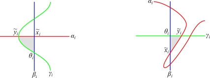
Figure 2. This show the domain of the Whitney triangle $\widetilde{\psi}$. For $i\in\{\ell+1,\ldots,d\}$, the curves $\beta_{i}$ and $\delta_{i}$ are small isotopic translates of each other, and – after isotoping $\alpha_{i}$ – we can find a “small” triangle bounded by $\alpha_{i}$, $\beta_{i}$, and $\delta_{i}$, shown shaded on the left. For $i\in\{1,\ldots,\ell\}$, after applying finger moves to the $\alpha$-curves, we can assume that there is a triangle, shown shaded on the right. The sum of all these triangles is the domain of $\widetilde{\psi}$.

By isotoping the $\alpha$-curves, we can create intersection points $\widetilde{\mathbf{x}}\in\mathbb{T}_{\alpha}\cap\mathbb{T}_{\beta}$ and $\widetilde{\mathbf{y}}\in\mathbb{T}_{\alpha}\cap\mathbb{T}_{\delta}$ such that there is a “small” triangle $\widetilde{\psi}\in\pi_{2}(\widetilde{\mathbf{x}},\theta,\widetilde{\mathbf{y}})$. The domain of $\widetilde{\psi}$ is shown in Figure 2. For each $i\in\{\ell+1,\ldots,d\}$, we isotope $\alpha_{i}$ – pushing the other $\alpha$-curves alongside – until it intersects both $\delta_{i}$ and $\beta_{i}$ near $\theta_{i}$, and consider the shaded triangle shown on the left-hand side of the figure. For each $i\in\{1,\ldots,\ell\}$, after some finger moves on the $\alpha$-curves – again, pushing the other $\alpha$-curves along – we can assume that there is a small triangle near each intersection point $\theta_{i}=\beta_{i}\cap\delta_{i}$, as shown shaded on the right-hand side of the figure. The sum of all these small triangles is the domain of the Whitney triangle $\widetilde{\psi}$. We denote by $\widetilde{\mathbf{x}}\in\mathbb{T}_{\alpha,\beta}$ and $\widetilde{\mathbf{y}}\in\mathbb{T}_{\alpha,\delta}$ the generators connected by $\widetilde{\psi}$; i.e., $\widetilde{\psi}\in\pi_{2}(\widetilde{\mathbf{x}},\theta,\widetilde{\mathbf{y}})$.

The Whitney triangle $\widetilde{\psi}$ satisfies $n_{z}(\widetilde{\psi})=n_{w}(\widetilde{\psi})=0$, but the constant $c$ is not necessarily defined for it, because $\mathfrak{s}(\widetilde{\mathbf{x}})$ and $\mathfrak{s}(\widetilde{\mathbf{y}})$ might not coincide with $\mathfrak{s}|_{Y_{\alpha,\beta}}$ and $\mathfrak{s}|_{Y_{\alpha,\delta}}$, respectively, where $\mathfrak{s}\in\text{Spin}^{c}(X)$ is the unique $\text{Spin}^{c}$ structure, cf. Equation (5.5). The next lemma proves that we can replace $\widetilde{\psi}$ with a Whitney triangle $\psi$ for which the constant $c$ is defined.

Lemma 5.22.

We can further isotope the $\alpha$-curves such that there is a Whitney triangle $\psi\in\pi_{2}(\mathbf{x},\theta,\mathbf{y})$ satisfying

• $n_{z}(\psi)=n_{w}(\psi)=0$ and

• $\mathfrak{s}(\mathbf{x})=\mathfrak{s}|_{Y_{\alpha,\beta}}$ and $\mathfrak{s}(\mathbf{y})=\mathfrak{s}|_{Y_{\alpha,\delta}}$.

Proof.

Given generators $\mathbf{x}^{\prime}=(x^{\prime}_{1},\ldots,x^{\prime}_{d})$ and $\mathbf{x}^{\prime\prime}=(x^{\prime\prime}_{1},\ldots,x^{\prime\prime}_{d})$ in $\mathbb{T}_{\alpha}\cap\mathbb{T}_{\beta}$, Ozsváth and Szabó associate to them [30, Definition 2.11] a class $\varepsilon(\mathbf{x}^{\prime},\mathbf{x}^{\prime\prime})\in H_{1}(Y_{\alpha,\beta})$. Choose 1-chains $a\subset\boldsymbol{\alpha}$ and $b\subset\boldsymbol{\beta}$ such that

$$\partial a=\partial b=x^{\prime\prime}_{1}+\cdots+x^{\prime\prime}_{d}-x^{\prime}_{1}-\cdots-x^{\prime}_{d}.$$

Then $a-b$ represents an element of $H_{1}(\Sigma)$ whose image in $H_{1}(Y_{\alpha,\beta})$ under the inclusion map is $\varepsilon(\mathbf{x}^{\prime},\mathbf{x}^{\prime\prime})$. Ozsváth and Szabó proved [30, Lemma 2.19] that

(5.6) $$\mathfrak{s}(\mathbf{x}^{\prime\prime})-\mathfrak{s}(\mathbf{x}^{\prime})=\operatorname{PD}(\varepsilon(\mathbf{x}^{\prime},\mathbf{x}^{\prime\prime})).$$

Consider the Whitney triangle $\widetilde{\psi}\in\pi_{2}(\widetilde{\mathbf{x}},\theta,\widetilde{\mathbf{y}})$ defined above, and whose domain is shown in Figure 2. Its domain is the disjoint union of $d$ triangles $\widetilde{T}_{1},\dots,\widetilde{T}_{d}$.

We define the homology classes $h_{1}\in H_{1}(Y_{\alpha,\beta})$ and $h_{2}\in H_{1}(Y_{\alpha,\delta})$ as

(5.7a) $$h_{1} =\operatorname{PD}\left(\mathfrak{s}|_{Y_{\alpha,\beta}}-\mathfrak{s}(\widetilde{\mathbf{x}})\right)\text{ and}$$

(5.7b) $$h_{2} =\operatorname{PD}\left(\mathfrak{s}|_{Y_{\alpha,\delta}}-\mathfrak{s}(\widetilde{\mathbf{y}})\right),$$

where $\mathfrak{s}$ is the unique $\text{Spin}^{c}$ structure on $X$. By Lemma 5.21, there is a homology class $h\in H_{1}(\Sigma)$ such that $i(h)=(h_{1},h_{2})$; i.e., $h$ represents $h_{1}$ in $H_{1}(Y_{\alpha,\beta})$ and $h_{2}$ in $H_{1}(Y_{\alpha,\delta})$. We can represent $h$ as $m\lambda$, where $\lambda$ is a simple closed curve on $\Sigma$ that satisfies the following conditions:

• $\lambda$ intersects the triangle $\widetilde{T}_{1}$ as on the left-hand side of Figure 3,

• $\lambda$ is disjoint from all the triangles $\widetilde{T}_{2},\ldots,\widetilde{T}_{d}$, and

• $\lambda$ is disjoint from the basepoints $z$ and $w$.

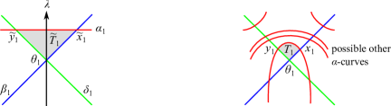
Figure 3. The picture above shows how to modify the Whitney triangle $\widetilde{\psi}$ defined in Figure 2 to obtain a Whitney triangle $\psi$ satisfying the requirements of Lemma 5.22. The picture on the left shows the loop $\lambda$ near the triangle $\widetilde{T}_{1}$. The picture on the right shows the new triangle $T_{1}$ in the triple Heegaard diagram obtained after performing a finger move on the $\alpha$-curves along $\lambda$.

If we perform a finger move on the $\alpha$-curves along the loop $m\lambda$, the result will look like the right-hand side of Figure 3. If $x_{1}$ and $y_{1}$ are as on the right-hand side of Figure 3, we define $\mathbf{x}=(x_{1},\widetilde{x}_{2},\ldots,\widetilde{x}_{d})$ and $\mathbf{y}=(y_{1},\widetilde{y}_{2},\ldots,\widetilde{y}_{d})$. Notice that, by construction,

(5.8) $$\varepsilon(\widetilde{\mathbf{x}},\mathbf{x})=h_{1}\text{ and }\varepsilon(\widetilde{\mathbf{y}},\mathbf{y})=h_{2}.$$

Let $\psi$ be a Whitney triangle with domain $T_{1}\sqcup\widetilde{T}_{2}\sqcup\cdots\sqcup\widetilde{T}_{d}$, where $T_{1}$ is the shaded triangle on the right-hand side of Figure 3. By construction, we have $n_{z}(\psi)=n_{w}(\psi)=0$. Furthermore, due to Equations (5.6), (5.8), and (5.7), we have

$$\mathfrak{s}(\mathbf{x}) =\mathfrak{s}(\widetilde{\mathbf{x}})+\operatorname{PD}(\varepsilon(\widetilde{\mathbf{x}},\mathbf{x}))$$

$$=\mathfrak{s}(\widetilde{\mathbf{x}})+\operatorname{PD}(h_{1})$$

$$=\mathfrak{s}(\widetilde{\mathbf{x}})+(\mathfrak{s}|_{Y_{\boldsymbol{\alpha},\boldsymbol{\beta}}}-\mathfrak{s}(\widetilde{\mathbf{x}}))=\mathfrak{s}|_{Y_{\alpha,\beta}}.$$

Analogously, we have $\mathfrak{s}(\mathbf{y})=\mathfrak{s}|_{Y_{\alpha,\delta}}$. ∎

Before showing that $c=0$ for the triangle $\psi\in\pi_{2}(\mathbf{x},\theta,\mathbf{y})$ constructed above, we prove that the relative $\text{Spin}^{c}$ structure $\mathfrak{s}^{\circ}(\psi)\in\text{Spin}^{c}(\mathcal{W}_{2})$ extends to a relative $\text{Spin}^{c}$ structure on $\mathcal{W}$.

Recall that $Y_{1}=Y_{\alpha,\beta}$ is obtained from $Y_{0}$ by performing surgery along some framed 0-spheres. The belt circles of the 1-handles involved give rise to embedded 2-spheres $O_{1},\dots,O_{p}\subset Y_{1}$. Similarly, $Y_{2}=Y_{\alpha,\delta}$ is obtained from $Y_{3}$ by surgery along some framed 0-spheres, giving rise to embedded spheres $O_{1}^{\prime},\dots,O_{s}^{\prime}\subset Y_{2}$. In Lemma 5.22, we achieved that $\mathfrak{s}(\mathbf{x})=\mathfrak{s}|_{Y_{\alpha,\beta}}$ and $\mathfrak{s}(\mathbf{y})=\mathfrak{s}|_{Y_{\alpha,\delta}}$. This implies that $\mathfrak{s}(\mathbf{x})$ extends to $X_{1}$, or equivalently, that $\langle\,c_{1}(\mathfrak{s}(\mathbf{x})),[O_{i}]\,\rangle=0$ for every $i\in\{1,\dots,p\}$. Similarly, $\langle\,c_{1}(\mathfrak{s}(\mathbf{y})),[O_{j}^{\prime}]\,\rangle=0$ for every $j\in\{1,\dots,s\}$. However

$$\langle\,c_{1}(\mathfrak{s}(\mathbf{x})),[O_{i}]\,\rangle=\langle\,c_{1}(\mathfrak{s}^{\circ}(\mathbf{x})),[O_{i}]\,\rangle=\langle\,c_{1}(\mathfrak{s}^{\circ}(\mathbf{x}),t),[O_{i}]\,\rangle,$$

as $\mathfrak{s}^{\circ}(\mathbf{x})$ and $\mathfrak{s}(\mathbf{x})$ are represented by the same vector field on $M_{1}\subset Y_{1}$. Since $M_{0}$ obtained from $M_{1}$ by compressing the 2-spheres $O_{1},\dots,O_{p}$, the equality

$$\langle\,c_{1}(\mathfrak{s}^{\circ}(\mathbf{x}),t),[O_{i}]\,\rangle=0$$

implies that $\mathfrak{s}^{\circ}(\mathbf{x})$ extends to $\mathfrak{s}^{\circ}_{1}\in\text{Spin}^{c}(\mathcal{W}_{1})$. Similarly, $\mathfrak{s}^{\circ}(\mathbf{y})$ extends to $\mathfrak{s}^{\circ}_{3}\in\text{Spin}^{c}(\mathcal{W}_{3})$. The Mayer-Vietoris sequence now implies that there is a $\text{Spin}^{c}$ structure $\mathfrak{s}^{\circ}\in\text{Spin}^{c}(\mathcal{W})$ such that $\mathfrak{s}^{\circ}|_{\mathcal{W}_{1}}=\mathfrak{s}^{\circ}_{1}$, $\mathfrak{s}^{\circ}|_{\mathcal{W}_{2}}=\mathfrak{s}^{\circ}(\psi)$, and $\mathfrak{s}^{\circ}|_{\mathcal{W}_{3}}=\mathfrak{s}^{\circ}_{3}$.

We are now ready to prove that, for the Whitney triangle $\psi$ constructed above, $c=0$. Recall that, by definition,

$$c=\mathcal{A}_{S_{2}}(\mathbf{y})-\mathcal{A}_{S_{1}}(\mathbf{x})=\langle c_{2}(\mathfrak{s}^{\circ}(\mathbf{y}),t),[S_{2}]\rangle-\langle c_{1}(\mathfrak{s}^{\circ}(\mathbf{x}),t),[S_{1}]\rangle,$$

cf. Equation (5.5), Definition 5.1, and Remark 5.2. Since $\psi$ is a Whitney triangle connecting $\mathbf{x}$, $\theta$, and $\mathbf{y}$, we have that $\mathfrak{s}^{\circ}(\psi)|_{M_{1}}=\mathfrak{s}^{\circ}(\mathbf{x})$ and $\mathfrak{s}^{\circ}(\psi)|_{M_{2}}=\mathfrak{s}^{\circ}(\mathbf{y})$, and therefore

$$c=\langle c_{1}(\mathfrak{s}^{\circ}(\psi),t),[S_{2}]\rangle-\langle c_{1}(\mathfrak{s}^{\circ}(\psi),t),[S_{1}]\rangle.$$

Notice that we can omit the restrictions of the (relative) $\text{Spin}^{c}$ structures by the naturality of Chern classes.

Now the relative $\text{Spin}^{c}$ structure $\mathfrak{s}^{\circ}(\psi)$ extends to some relative $\text{Spin}^{c}$ structure $\mathfrak{s}^{\circ}\in\text{Spin}^{c}(\mathcal{W})$ by the above. Then, by Lemmas 5.8 and 5.11, we have

$$c=\langle c_{1}(\mathfrak{s}^{\circ},t),[S_{3}]\rangle-\langle c_{1}(\mathfrak{s}^{\circ},t),[S_{0}]\rangle.$$

From Lemma 3.9, it finally follows that $c=0$.

We can now conclude the proof of Lemma 5.13. By Equation (5.5), for any Whitney triangle $\psi\in\pi_{2}(\mathbf{x},\theta,\mathbf{y})$, where $\mathbf{x}\in\mathbb{T}_{\alpha}\cap\mathbb{T}_{\beta}$ and $\mathbf{y}\in\mathbb{T}_{\alpha}\cap\mathbb{T}_{\delta}$ are such that $\mathfrak{s}(\mathbf{x})$ and $\mathfrak{s}(\mathbf{y})$ extend to $X_{1}$ and $X_{3}$, respectively, we have

$$\mathcal{A}_{S_{2}}(\mathbf{y})-\mathcal{A}_{S_{1}}(\mathbf{x})+n_{z}(\psi)-n_{w}(\psi)=0.$$

If $\psi$ contributes to the surgery map $f_{\mathcal{H}^{1},\mathbb{L}}(\mathbf{x})$, then $n_{w}(\psi)=0$, and it has a pseudo-holomorphic representative, so $n_{z}(\psi)\geq 0$. Consequently, $A_{S_{2}}(\mathbf{y})\leq A_{S_{1}}(\mathbf{x})$, as desired. ∎

5.11. Naturality maps

Recall that [17], given two admissible Heegaard diagrams $\mathcal{H}$ and $\mathcal{H}^{\prime}$ for the same 3-manifold $Y$, there is a naturality map

$$f_{\mathcal{H},\mathcal{H}^{\prime}}\colon\widehat{\mathit{CF}}(\mathcal{H})\longrightarrow\widehat{\mathit{CF}}(\mathcal{H}^{\prime}),$$

which is the composition of maps associated to isotopies of the attaching sets, handleslides, (de)stabilisations, and diffeomorphisms of the Heegaard surface isotopic to the identity in $Y$. On the homology, it induces an isomorphism

$$F_{\mathcal{H},\mathcal{H}^{\prime}}\colon\widehat{\mathit{HF}}(\mathcal{H})\to\widehat{\mathit{HF}}(\mathcal{H}^{\prime})$$

that is independent of the sequence of Heegaard moves.

In our case, $\mathcal{H}$ and $\mathcal{H}^{\prime}$ are doubly pointed Heegaard diagrams, which define the same decorated knot $(Y,K,P)$. Together with Dylan Thurston, the first author proved [17, Proposition 2.37] that $\mathcal{H}$ and $\mathcal{H}^{\prime}$ can be connected by a sequence of Heegaard moves that do not cross the basepoints $w$ and $z$. If we forget about the $z$ basepoint, this sequence induces the naturality map $f_{\mathcal{H},\mathcal{H}^{\prime}}\colon\widehat{\mathit{CF}}(\mathcal{H})\to\widehat{\mathit{CF}}(\mathcal{H}^{\prime})$ above. As we explained, the $z$ basepoints on $\mathcal{H}$ and $\mathcal{H}^{\prime}$ induce filtrations on $\widehat{\mathit{CF}}(\mathcal{H})$ and $\widehat{\mathit{CF}}(\mathcal{H}^{\prime})$. It follows from the work of Ozsváth-Szabó [29] and Rasmussen [32] that, if $f_{\mathcal{H},\mathcal{H}^{\prime}}$ is the map associated to either an isotopy, a handleslide, a (de)stabilization, or a diffeomorphism of the Heegaard surface isotopic to the identity in $Y$, then it preserves the knot filtration. If $f_{\mathcal{H},\mathcal{H}^{\prime}}$ is an isotopy map or a handleslide map, then the map induced on the $E^{1}$ page is the corresponding naturality map $F_{\mathcal{H},\mathcal{H}^{\prime}}$ on $\widehat{\mathit{HFK}}$; i.e., it is the map obtained by counting all holomorphic triangles that do not cross $z$. If $f_{\mathcal{H},\mathcal{H}^{\prime}}$ is a (de)stabilization or diffeomorphism map, then it is an isomorphism of filtered complexes.

As the above result is only outlined in the works of Ozsváth and Szabó [29] and Rasmussen [32], we provide a bit more detail. With the techniques of this paper, we can prove the following analogue of Lemma 5.13.

Lemma 5.23.

Let $K$ be a null-homologous knot in $Y=\#_{i=1}^{p}(S^{1}\times S^{2}).$ Choose a Seifert surface $S$ for $K$. Suppose that $\mathcal{H}$ and $\mathcal{H}^{\prime}$ are admissible doubly pointed Heegaard diagrams for $(Y,K,P)$ that only differ by an isotopy or a handleslide.

Given an admissible doubly pointed triple diagram $(\Sigma,\boldsymbol{\alpha},\boldsymbol{\beta},\boldsymbol{\delta},w,z)$ for the Heegaard move $\mathcal{H}\to\mathcal{H}^{\prime}$, if $\mathbf{x}\in\mathbb{T}_{\alpha}\cap\mathbb{T}_{\beta}$, then for any $\mathbf{y}\in\mathbb{T}_{\alpha}\cap\mathbb{T}_{\delta}$ that has non-trivial coefficient in the expansion of $f_{\mathcal{H},\mathcal{H}^{\prime}}(\mathbf{x})$, we have that

$$\mathcal{F}_{S}(\mathbf{y})\leq\mathcal{F}_{S}(\mathbf{x}).$$

Furthermore, if $\psi$ is a holomorphic triangle connecting $\mathbf{x}\in\mathbb{T}_{\alpha}\cap\mathbb{T}_{\beta}$, $\theta\in\mathbb{T}_{\beta}\cap\mathbb{T}_{\delta}$ (the top-dimensional generator of $\widehat{\mathit{CF}}(\Sigma,\boldsymbol{\beta},\boldsymbol{\delta},w,z)$), and $\mathbf{y}\in\mathbb{T}_{\alpha}\cap\mathbb{T}_{\delta}$ that does not cross $w$, then

(5.9) $$\mathcal{F}_{S}(\mathbf{y})=\mathcal{F}_{S}(\mathbf{x})-n_{z}(\psi).$$

Remark 5.24.

The (de)stabilization and diffeomorphism maps do not appear in Lemma 5.23 because they are not triangle maps. They are already isomorphisms at the level of filtered chain complexes.

Idea of the proof.

As in the proof of Lemma 5.13, we let

$$c=\mathcal{A}_{S}(\mathbf{y})-\mathcal{A}_{S}(\mathbf{x})-n_{w}(\psi)+n_{z}(\psi),$$

and prove that this is independent of $\psi$, $\mathbf{x}$, and $\mathbf{y}$. The main differences from the proof of Lemma 5.13 are the following:

• Triply periodic domains: We closely follow the proof of Proposition 5.16. In this case, $X\cong Y\times I$, the boundary of the 4-manifold $X_{\triangle}$ consists of $Y\sqcup Y\sqcup Y_{\boldsymbol{\beta},\boldsymbol{\delta}}$, and the cobordisms $X_{1}$ and $X_{3}$ are replaced by identity cobordisms $Y\times I$. Finally, the proof of the injectivity of $\varphi$ follows from the surjectivity of the map

  $$\rho\colon H_{2}(Y\times I)\oplus H_{2}(Y\times I)\oplus H_{2}(\widehat{X})\longrightarrow H_{2}(X),$$

  as noted in Remark 5.19.

• Doubly periodic domains: One can use Proposition 5.20 for the two copies of $Y$ and for $Y_{\boldsymbol{\beta},\boldsymbol{\delta}}$.

• Proving that $c=0$: This is easier than in the case of the $2$-handle maps, because we already know that the naturality map preserves the graded Euler characteristic, and this forces the grading shift $c$ to be $0$. Also, as $X_{1}$ and $X_{3}$ are products, $\text{Spin}^{c}$ structures automatically extend to them, hence we do not need to isotope the $\alpha$-curves. ∎

5.12. Proof of Theorem 5.4

We are now ready to prove Theorem 5.4. In the proof we use the notation introduced in Section 5.4, and we assume that the gluing map is the identity map, as explained in Section 5.3.

Suppose that $\mathbf{x}$ is a generator of $\widehat{\mathit{CF}}(\mathcal{H}^{0})$ such that $f_{\mathcal{C}}(\mathbf{x})\neq 0$. Let $\mathbf{y}$ be a generator of $\widehat{\mathit{CF}}(\mathcal{H}^{2}_{\mathbb{S}})$ that appears in the expression of $f_{\mathcal{C}}(\mathbf{x})$ with non-zero coefficient. Then there exist generators $\mathbf{x}^{\prime}\in\widehat{\mathit{CF}}(\mathcal{H}^{0}_{\mathbb{P}})$, $\mathbf{x}^{\prime\prime}\in\widehat{\mathit{CF}}(\mathcal{H}^{1})$, $\mathbf{y}^{\prime\prime}\in\widehat{\mathit{CF}}(\mathcal{H}^{1}_{\mathbb{L}})$, and $\mathbf{y}^{\prime}\in\widehat{\mathit{CF}}(\mathcal{H}^{2})$ that appear with non-zero coefficient in $f_{\mathcal{H}^{0},\mathbb{P}}(\mathbf{x})$, $f_{\mathcal{H}^{0}_{\mathbb{P}},\mathcal{H}_{1}}(\mathbf{x}^{\prime})$, $f_{\mathcal{H}^{1},\mathbb{L}}(\mathbf{x}^{\prime\prime})$, and $f_{\mathcal{H}^{1}_{\mathbb{L}},\mathcal{H}^{2}}(\mathbf{y}^{\prime\prime})$, respectively, and such that $\mathbf{y}$ appears with non-zero coefficient in $f_{\mathcal{H}^{2},\mathbb{S}}(\mathbf{y}^{\prime})$. Notice that, by construction, $\mathfrak{s}(\mathbf{x}^{\prime\prime})$ extends to $X_{1}$ and $\mathfrak{s}(\mathbf{y}^{\prime\prime})$ extends to $X_{3}$.

By Lemma 5.23, we know that the naturality maps preserve the knot filtration, and by Corollaries 5.10 and 5.12 so do the maps $f_{\mathcal{H}^{0},\mathbb{P}}$ and $f_{\mathcal{H}^{2},\mathbb{S}}$. Finally, Lemma 5.13 proves that $\mathcal{F}_{S_{2}}(\mathbf{y}^{\prime\prime})\leq\mathcal{F}_{S_{1}}(\mathbf{x}^{\prime\prime})$. By putting all these together, we obtain that

(5.10) $$\mathcal{F}_{S_{3}}(\mathbf{y})=\mathcal{F}_{S_{2}}(\mathbf{y}^{\prime})\leq\mathcal{F}_{S_{2}}(\mathbf{y}^{\prime\prime})\leq\mathcal{F}_{S_{1}}(\mathbf{x}^{\prime\prime})\leq\mathcal{F}_{S_{1}}(\mathbf{x}^{\prime})=\mathcal{F}_{S_{0}}(\mathbf{x}).$$

Thus $f_{\mathcal{C}}$ is a map of filtered complexes and so, by Remark 4.6, it induces a morphism of spectral sequences.

Furthermore, each of the maps $f_{\mathcal{H}^{0},\mathbb{P}}$, $f_{\mathcal{H}^{0}_{\mathbb{P}},\mathcal{H}^{1}}$, $f_{\mathcal{H}^{1},\mathbb{L}}$, $f_{\mathcal{H}^{1}_{\mathbb{L}},\mathcal{H}^{2}}$, and $f_{\mathcal{H}^{2},\mathbb{S}}$ is a map of filtered complexes. The map induced by $f_{\mathcal{C}}$ on the $E^{1}$ page is the composition of the maps induced by each of the above maps on the $E^{1}$ page.

We now consider the case when the inequalities in Equation (5.10) are all equalities. Lemmas 5.8 and 5.11 imply that the maps induced by $f_{\mathcal{H}^{0},\mathbb{P}}$ and $f_{\mathcal{H}^{2},\mathbb{S}}$ on the $E^{1}$ page are the 1- and 3-handle maps for $\widehat{\mathit{HFK}}$. As for the 2-handle map $f_{\mathcal{H}^{1},\mathbb{L}}$, by Equation (5.3) in Lemma 5.13, we have that $\mathcal{F}(\mathbf{y}^{\prime\prime})=\mathcal{F}(\mathbf{x}^{\prime\prime})$ if and only if there is a pseudo-holomorphic triangle $\psi$ connecting $\mathbf{x}^{\prime\prime}$, $\theta$, and $\mathbf{y}^{\prime\prime}$ such that $n_{w}(\psi)=n_{z}(\psi)=0$, and in this case all such holomorphic triangles satisfy this equality. Hence, the map induced by $f_{\mathcal{H}^{1},\mathbb{L}}$ on the $E^{1}$ page is the 2-handle map for $\widehat{\mathit{HFK}}$. Finally, it follows from the discussion in Section 5.11 that the maps induced on the $E^{1}$ page by the naturality maps for $\widehat{\mathit{CF}}$ are the naturality maps for $\widehat{\mathit{HFK}}$. Alternatively, one can use Equation (5.9) in Lemma 5.23 and argue in the same way as for the 2-handle maps.

This immediately implies that the map induced by $f_{\mathcal{C}}$ on the $E^{1}$ page is obtained by counting (for the naturality maps and the 2-handle map) the pseudo-holomorphic triangles that do not cross $w$ and $z$, and so it is $F_{\mathcal{C}}$.

On the other hand, the map induced by $f_{\mathcal{C}}$ on the total homology is given by counting all holomorphic triangles that do not cross $w$ but might cross $z$. This is precisely the map $\widehat{F}_{X}\colon\widehat{\mathit{HF}}(S^{3})\to\widehat{\mathit{HF}}(S^{3})$ induced by the cobordism $X$. Since $H_{1}(X)=H_{2}(X)=0$, the map $\widehat{F}_{X}=\text{Id}_{\widehat{\mathit{HF}}(S^{3})}$ by [27, Lemma 3.4]. ∎

6. Concordance maps preserve the homological grading

In this section, we show that concordance maps also behave well with respect to another grading of $\widehat{\mathit{CF}}$, namely the homological grading.

Let $\mathcal{H}$ be an admissible pointed Heegaard diagram for the closed, connected, oriented, based 3-manifold $(Y,w)$, together with a $\text{Spin}^{c}$ structure $\mathfrak{s}\in\text{Spin}^{c}(Y)$ such that $c_{1}(\mathfrak{s})\in H^{2}(Y)$ is torsion. Ozsváth and Szabó [30, Section 4] showed that $\widehat{\mathit{CF}}(\mathcal{H},\mathfrak{s})$ admits a relative $\mathbb{Z}$-grading. For generators $\mathbf{x}$, $\mathbf{y}\in\widehat{\mathit{CF}}(\mathcal{H},\mathfrak{s})$ and $\phi\in\pi_{2}(\mathbf{x},\mathbf{y})$, we have

(6.1) $$\mathit{gr}(\mathbf{x},\mathbf{y})=\mu(\phi)-2n_{w}(\phi).$$

They showed [31, Theorem 7.1] that this can be lifted to an absolute $\mathbb{Q}$-grading $\widetilde{\mathit{gr}}$, in the sense that $\mathit{gr}(\mathbf{x},\mathbf{y})=\widetilde{\mathit{gr}}(\mathbf{x})-\widetilde{\mathit{gr}}(\mathbf{y})$. Such a grading is called the Maslov grading or homological grading.

Example 6.1.

If $Y=S^{3}$ with its unique $\text{Spin}^{c}$ structure $\mathfrak{s}_{0}$, and if $\mathcal{H}$ is a Heegaard diagram of $Y$, then on $\widehat{\mathit{CF}}(\mathcal{H},\mathfrak{s}_{0})$ the absolute $\mathbb{Q}$-grading is actually an absolute $\mathbb{Z}$-grading. The generator of $\widehat{\mathit{HF}}(S^{3},\mathfrak{s}_{0})\cong\mathbb{Z}_{2}$ is homogeneous of grading zero.

More generally, if $Y=\#_{i=1}^{k}(S^{1}\times S^{2})$ with Heegaard diagram $\mathcal{H}$, and $\mathfrak{s}_{0}\in\text{Spin}^{c}(Y)$ is such that $c_{1}(\mathfrak{s}_{0})=0$, then $\widetilde{\mathit{gr}}$ is an absolute $\mathbb{Z}$-grading on $\widehat{\mathit{CF}}(\mathcal{H},\mathfrak{s}_{0})$.

The main result of this section is the following.

Theorem 6.2.

Let $\mathcal{C}$ be a decorated concordance from $(S^{3},K_{0},P_{0})$ to $(S^{3},K_{1},P_{1})$, and let $\mathcal{H}_{i}$ be an admissible doubly pointed diagram of $(S^{3},K_{i},P_{i})$ for $i\in\{0,1\}$. Then, the chain map

$$f_{\mathcal{C}}\colon\widehat{\mathit{CF}}(\mathcal{H}_{0})\longrightarrow\widehat{\mathit{CF}}(\mathcal{H}_{1})$$

preserves the absolute homological grading; that is, if $x\in\widehat{\mathit{CF}}(\mathcal{H}_{0})$ is $\widetilde{\mathit{gr}}$-homogeneous, so is $f_{\mathcal{C}}(x)$, and if $f_{\mathcal{C}}(x)\neq 0$, then

$$\widetilde{\mathit{gr}}(f_{\mathcal{C}}(x))=\widetilde{\mathit{gr}}(x).$$

Remark 6.3.

Notice that the statement of Theorem 6.2 is stronger than the fact that $f_{\mathcal{C}}$ preserves the Maslov filtration. We actually claim that the Maslov grading is not decreased by $f_{\mathcal{C}}$.

Idea of the proof.

We proceed similarly to the proof of Theorem 5.4, and use the notation from Section 5.4 and Figure 1. As the diffeomorphism $D$ constructed in Section 5.3 induces a homomorphism $D_{*}$ that preserves the homological grading, we can assume the gluing map is trivial and we are dealing with a special cobordism.

First, we prove that, in the right $\text{Spin}^{c}$ structure, each map $f_{\mathcal{H}^{0},\mathbb{P}}$, $f_{\mathcal{H}^{0}_{\mathbb{P}},\mathcal{H}^{1}}$, $f_{\mathcal{H}^{1},\mathbb{L}}$, $f_{\mathcal{H}^{1}_{\mathbb{L}},\mathcal{H}^{2}}$, and $f_{\mathcal{H}^{2},\mathbb{S}}$ preserves the relative Maslov grading $\mathit{gr}$. This is only implicit in the work of Ozsváth and Szabó [31], so we provide more detail. Then we show that the absolute grading shift of $f_{\mathcal{C}}$, which is the composition of all the above maps, is zero.

For the 1- and 3-handle maps $f_{\mathcal{H}^{0},\mathbb{P}}$ and $f_{\mathcal{H}^{2},\mathbb{S}}$, it is straightforward to check that the relative Maslov grading is preserved using Equation (6.1) above.

Now consider the 2-handle map $f_{\mathcal{H}^{1},\mathbb{L}}$. Let $(\Sigma,\boldsymbol{\alpha},\boldsymbol{\beta},\boldsymbol{\delta},w,z)$ be an admissible triple Heegaard diagram subordinate to a bouquet for $\mathbb{L}$. For generators $\mathbf{x}\in\mathbb{T}_{\alpha}\cap\mathbb{T}_{\beta}$ and $\mathbf{y}\in\mathbb{T}_{\alpha}\cap\mathbb{T}_{\delta}$ such that $\mathfrak{s}(\mathbf{x})=\mathfrak{s}|_{Y_{\alpha,\beta}}$ and $\mathfrak{s}(\mathbf{y})=\mathfrak{s}|_{Y_{\alpha,\delta}}$, where $\mathfrak{s}$ denotes the unique $\text{Spin}^{c}$ structure on $X$, and for every Whitney triangle $\psi\in\pi_{2}(\mathbf{x},\theta,\mathbf{y})$, we let

$$d=\widetilde{\mathit{gr}}(\mathbf{y})-\widetilde{\mathit{gr}}(\mathbf{x})+\mu(\psi)-2n_{w}(\psi).$$

We show that $d$ is independent of $\psi$, $\mathbf{x}$, and $\mathbf{y}$. Since the triangles $\psi$ contributing to $f_{\mathcal{H}^{1},\mathbb{L}}$ have $\mu(\psi)=0$ and $n_{w}(\psi)=0$, it follows that the absolute grading is shifted by $d$, so the relative grading is preserved.

We already know from the work of Ozsváth and Szabó [30] that the naturality maps $f_{\mathcal{H}^{0}_{\mathbb{P}},\mathcal{H}^{1}}$ and $f_{\mathcal{H}^{1}_{\mathbb{L}},\mathcal{H}^{2}}$ preserve the relative homological grading $\mathit{gr}$. Alternatively, this can also be shown using the techniques of Section 5.11.

Finally, $f_{\mathcal{C}}$, which is the composition of all the above maps, preserves the relative homological grading, or equivalently, it shifts the absolute homological grading by some constant $e$. This implies that, for every $r\in\mathbb{N}$, the map $E^{r}(f_{\mathcal{C}})$ shifts the homological grading by the same constant $e$ independent of $r$. Since we know that the map in total homology is $\text{Id}_{\widehat{\mathit{HF}}(S^{3})}$ and preserves the absolute grading by [27, Lemma 3.4], it immediately follows that $e=0$. ∎

The rest of this section is devoted to filling in the details of the above outline.

6.1. $\text{Spin}^{c}$ structures

Let $\mathfrak{s}$ be the unique $\text{Spin}^{c}$ structure on $X$. Then

$$f_{\mathcal{C}}=f_{\mathcal{C},\mathfrak{s}}=f_{\mathcal{H}^{2},\mathbb{S},\mathfrak{s}}\circ\cdots\circ f_{\mathcal{H}^{0},\mathbb{P},\mathfrak{s}},$$

where the restrictions of $\mathfrak{s}$ are omitted for the sake of clarity.

So it suffices to consider the above maps in the $\text{Spin}^{c}$ structure $\mathfrak{s}$. In the rest of the section, we will focus on the maps $f_{\mathcal{H}^{2},\mathbb{S},\mathfrak{s}},\ldots,f_{\mathcal{H}^{0},\mathbb{P},\mathfrak{s}}$, and for simplicity, we will denote the restrictions of $\mathfrak{s}$ by the same letter.

6.2. 1- and 3-handles

The 1-handle map $f_{\mathcal{H}^{0},\mathbb{P},\mathfrak{s}}$ satisfies the following.

Lemma 6.4.

Let $\mathbf{x}^{\prime\prime}$, $\widetilde{\mathbf{x}}^{\prime\prime}\in\widehat{\mathit{CF}}(\mathcal{H}^{0},\mathfrak{s})$ be generators. Then

$$\mathit{gr}(\mathbf{x}^{\prime\prime},\widetilde{\mathbf{x}}^{\prime\prime})=\mathit{gr}(f_{\mathcal{H}^{0},\mathbb{P},\mathfrak{s}}(\mathbf{x}^{\prime\prime}),f_{\mathcal{H}^{0},\mathbb{P},\mathfrak{s}}(\widetilde{\mathbf{x}}^{\prime\prime}));$$

i.e., the relative homological grading is preserved under the 1-handle map.

Proof.

Let $\phi\in\pi_{2}(\mathbf{x}^{\prime\prime},\widetilde{\mathbf{x}}^{\prime\prime})$. Then the domain of $\phi$ also represents a Whitney disk between $f_{\mathcal{H}^{0},\mathbb{P}}(\mathbf{x}^{\prime\prime})$ and $f_{\mathcal{H}^{0},\mathbb{P}}(\widetilde{\mathbf{x}}^{\prime\prime})$ in the Heegaard diagram $\mathcal{H}^{0}_{\mathbb{P}}$ that we also denote by $\phi$. By Equation (6.1), we have

$$\mathit{gr}(\mathbf{x}^{\prime\prime},\widetilde{\mathbf{x}}^{\prime\prime})=\mu(\phi)-2n_{w}(\phi)=\mathit{gr}(f_{\mathcal{H}^{0},\mathbb{P},\mathfrak{s}}(\mathbf{x}^{\prime\prime}),f_{\mathcal{H}^{0},\mathbb{P},\mathfrak{s}}(\widetilde{\mathbf{x}}^{\prime\prime})).\qed$$

A dual argument gives the following result for the 3-handle map $f_{\mathcal{H}^{2},\mathbb{S},\mathfrak{s}}$.

Lemma 6.5.

Let $\mathbf{y}^{\prime}$, $\widetilde{\mathbf{y}}^{\prime}\in\widehat{\mathit{CF}}(\mathcal{H}^{2},\mathfrak{s})$ be generators such that $f_{\mathcal{H}^{2},\mathbb{S},\mathfrak{s}}(\mathbf{y}^{\prime})\neq 0$ and $f_{\mathcal{H}^{2},\mathbb{S},\mathfrak{s}}(\widetilde{\mathbf{y}}^{\prime})\neq 0$. Then

$$\mathit{gr}(\mathbf{y}^{\prime},\widetilde{\mathbf{y}}^{\prime})=\mathit{gr}(f_{\mathcal{H}^{2},\mathbb{S},\mathfrak{s}}(\mathbf{y}^{\prime}),f_{\mathcal{H}^{2},\mathbb{S},\mathfrak{s}}(\widetilde{\mathbf{y}}^{\prime}));$$

i.e., the relative homological grading is preserved under the 3-handle map.

6.3. 2-handles

For 2-handles, we have the following.

Lemma 6.6.

Let $\mathbf{x}$, $\widetilde{\mathbf{x}}\in\widehat{\mathit{CF}}(\mathcal{H}^{1})$ be generators such that $\mathfrak{s}(\mathbf{x})=\mathfrak{s}(\widetilde{\mathbf{x}})=\mathfrak{s}$. Then $f_{\mathcal{H}^{1},\mathbb{L},\mathfrak{s}}(\mathbf{x})$ and $f_{\mathcal{H}^{1},\mathbb{L},\mathfrak{s}}(\widetilde{\mathbf{x}})$ are $\widetilde{\mathit{gr}}$-homogeneous, and if they are non-zero, then

$$\mathit{gr}(\mathbf{x},\widetilde{\mathbf{x}})=\mathit{gr}(f_{\mathcal{H}^{1},\mathbb{L},\mathfrak{s}}(\mathbf{x}),f_{\mathcal{H}^{1},\mathbb{L},\mathfrak{s}}(\widetilde{\mathbf{x}})).$$

Proof.

For $\mathbf{x}\in\widehat{\mathit{CF}}(\mathcal{H}^{1})$, $\mathbf{y}\in\widehat{\mathit{CF}}(\mathcal{H}^{1}_{\mathbb{L}})$, and $\psi\in\pi_{2}(\mathbf{x},\theta,\mathbf{y})$ such that $\mathfrak{s}(\psi)=\mathfrak{s}$, let

(6.2) $$d=\widetilde{\mathit{gr}}(\mathbf{y})-\widetilde{\mathit{gr}}(\mathbf{x})+\mu(\psi)-2n_{w}(\psi).$$

First, we check that $d$ is independent of $\psi$. As in the proof of Lemma 5.13, it suffices to show that, for every triply periodic domain $\mathcal{P}$,

(6.3) $$\mu(\mathcal{P})=2n_{w}(\mathcal{P}).$$

Since every triply periodic domain is the sum of doubly periodic domains by Proposition 5.16, it is sufficient to prove Equation (6.3) in the case of doubly periodic domains in Heegaard diagrams of $Y_{\alpha,\beta}$, $Y_{\alpha,\delta}$, and $Y_{\beta,\delta}$.

Consider, for example, $Y_{\alpha,\beta}$ and $\mathbf{z}\in\mathbb{T}_{\alpha}\cap\mathbb{T}_{\beta}$, with a periodic domain $\mathcal{P}\in\Pi_{\alpha,\beta}$ based at $\mathbf{z}$. As $\mathfrak{s}(\mathbf{z})$ extends to the cobordism $X_{1}$, we see that $c_{1}(\mathfrak{s}(\mathbf{z}))$ vanishes on the belt spheres of the 1-handles. Furthermore, since $H(\mathcal{P})\in H_{2}(Y)$ is a linear combination of the belt spheres, we obtain that

$$\langle\,c_{1}(\mathfrak{s}(\mathbf{z})),H(\mathcal{P})\,\rangle=0.$$

By the work of Ozsváth and Szabó [30, Theorem 4.9] and Lipshitz [20, Lemma 4.10],

$$\mu(\mathcal{P})=\langle\,c_{1}(\mathfrak{s}(\mathbf{z})),H(\mathcal{P})\,\rangle+2n_{w}(\mathcal{P}),$$

and the result follows. This proves that $d$ is independent of $\psi$.

Next, we check that $d$ is independent of $\mathbf{x}$ and $\mathbf{y}$. Let $\widetilde{\mathbf{x}}$ be another generator of $\widehat{\mathit{CF}}(\mathcal{H}^{1})$ such that $\mathfrak{s}(\widetilde{\mathbf{x}})=\mathfrak{s}$. Then there is a Whitney disk $\phi\in\pi_{2}(\widetilde{\mathbf{x}},\mathbf{x})$, hence $\phi\#\psi\in\pi_{2}(\widetilde{\mathbf{x}},\theta,\mathbf{y})$. Then, by Equation (6.1),

$$\begin{split}d&=\widetilde{\mathit{gr}}(\mathbf{y})-\widetilde{\mathit{gr}}(\mathbf{x})+\mu(\psi)-2n_{w}(\psi)\\ &=\widetilde{\mathit{gr}}(\mathbf{y})-\widetilde{\mathit{gr}}(\mathbf{x})+\mu(\psi)-2n_{w}(\psi)+(\widetilde{\mathit{gr}}(\mathbf{x})-\widetilde{\mathit{gr}}(\widetilde{\mathbf{x}})+\mu(\phi)-2n_{w}(\phi))\\ &=\widetilde{\mathit{gr}}(\mathbf{y})-\widetilde{\mathit{gr}}(\widetilde{\mathbf{x}})+\mu(\phi\#\psi)-2n_{w}(\phi\#\psi).\end{split}$$

Thus, $d$ is independent of $\mathbf{x}$. An analogous argument shows independence of $\mathbf{y}$.

Finally, all the holomorphic triangles that appear in the definition of the map $f_{\mathcal{H}^{1},\mathbb{L},\mathfrak{s}}$ satisfy $\mu(\psi)=0$ and $n_{w}(\psi)=0$. Then, it follows from Equation (6.2) that $f_{\mathcal{H}^{1},\mathbb{L},\mathfrak{s}}$ increases the absolute grading $\widetilde{\mathit{gr}}$ by $d$. In particular, it preserves the relative grading $\mathit{gr}$. ∎

6.4. Naturality maps

We already know from the work of Ozsváth and Szabó [30] that the naturality maps preserve the Maslov grading. Alternatively, one can prove that the handleslide and isotopy maps preserve the Maslov grading using the techniques of Lemma 6.6. The (de)stabilization maps are already isomorphisms on the chain level.

6.5. Proof of Theorem 6.2

As explained in Section 6.1,

$$f_{\mathcal{C}}=f_{\mathcal{H}^{2},\mathbb{S},\mathfrak{s}}\circ f_{\mathcal{H}^{1}_{\mathbb{L}},\mathcal{H}^{2},\mathfrak{s}}\circ f_{\mathcal{H}^{1},\mathbb{L},\mathfrak{s}}\circ f_{\mathcal{H}^{0}_{\mathbb{P}},\mathcal{H}^{1},\mathfrak{s}}\circ f_{\mathcal{H}^{0},\mathbb{P},\mathfrak{s}}.$$

All the above maps preserve the relative Maslov grading by Lemmas 6.4, 6.5 and 6.6, so $f_{\mathcal{C}}$ shifts the absolute Maslov grading by some constant $e$. It follows that the maps induced between the spectral sequences $E^{r}(f_{\mathcal{C}})$ shift the absolute Maslov grading by the same constant $e$. On the other hand, the map in total homology is $\text{Id}_{\widehat{\mathit{HF}}(S^{3})}$, which is homogeneous of degree $0$, so we obtain that $e=0$. ∎

References

- [1] G. Arone and M. Kankaanrinta, On the functoriality of the blow-up construction, Bull. Belg. Math. Soc. Simon Stevin 17 (2010), no. 5, 821–832.
- [2] M. Atiyah, Topological quantum field theories, Inst. Hautes Études Sci. Publ. Math. 68 (1988), 175–186.
- [3] J. Baldwin and W. Gillam, Computations of Heegaard-Floer knot homology, J. Knot Theory Ramifications 21 (2012), no. 8, 65 pages.
- [4] C. Blanchet and V. Turaev, Axiomatic approach to TQFT, Encyclopedia of Mathematical Physics, Elsevier, 2006, pp. 232–234.
- [5] R. Fox, Some problems in knot theory, Topology of 3-manifolds and Related Topics, Prentice-Hall, 1962, pp. 168–176.
- [6] M. Freedman, R. Gompf, S. Morrison, and K. Walker, Man and machine thinking about the smooth 4-dimensional Poincaré conjecture, Quantum Topol. 1 (2010), no. 2, 171–208.
- [7] D. Gabai, Foliations and the topology of 3-manifolds, J. Differential Geom. 18 (1983), 445–503.
- [8] P. Ghiggini, Knot Floer homology detects genus-one fibred knots, Amer. J. Math. 130 (2008), no. 5, 1151–1169.
- [9] M. Hedden, On knot Floer homology and cabling, PhD Thesis, Columbia University (2005).
- [10] K. Honda, On the classification of tight contact structures. II., J. Differential Geom. 55 (2000), no. 1, 83–143.
- [11] K. Honda, W. Kazez, and G. Matić, Contact structures, sutured Floer homology and TQFT, math.GT/0807.2431.
- [12] M. Jacobsson, An invariant of link cobordisms from Khovanov homology, Algebr. Geom. Topol. 4 (2004), 1211–1251.
- [13] A. Juhász, Holomorphic discs and sutured manifolds, Algebr. Geom. Topol. 6 (2006), 1429–1457.
- [14] by same author, Floer homology and surface decompositions, Geom. Topol. 12 (2008), 299–350.
- [15] by same author, The sutured Floer homology polytope, Geom. Topol. 14 (2010), 1303–1354.
- [16] by same author, Cobordisms of sutured manifolds and the functoriality of link floer homology, arXiv:0910.4382 (2015).
- [17] A. Juhász and D. Thurston, Naturality and mapping class groups in Heegaard Floer homology, math.GT/1210.4996.
- [18] C. Karakurt and T. Lidman, Rank inequalities for the Heegaard Floer homology of Seifert homology spheres, arXiv:1310.0760 (2013).
- [19] P. Kronheimer and T. Mrowka, Gauge theory and Rasmussen’s invariant, J. Topol. 6 (2013), no. 3, 659–674.
- [20] R. Lipshitz, A cylindrical reformulation of Heegaard Floer homology, Geom. Topol. 10 (2006), 955–1097.
- [21] R. Lutz, Structures de contact sur les fibrés principaux en cercles de dimension trois, Ann. Inst. Fourier 27 (1977), no. 3, 1–15.
- [22] C. Manolescu and P. Ozsváth, On the Khovanov and knot Floer homologies of quasi-alternating links, Proceedings of Gökova Geometry-Topology Conference 2007 (2008), 60–81.
- [23] C. Manolescu, P. Ozsváth, and S. Sarkar, A combinatorial description of knot Floer homology, Ann. of Math. 169 (2009), 633–660.
- [24] J. McCleary, A user’s guide to spectral sequences, Cambridge Studies in Advanced Mathematics, Cambridge University Press, 2001.
- [25] Y. Ni, Knot Floer homology detects fibred knots, Invent. Math. 170 (2007), 577–608.
- [26] by same author, Erratum: Knot Floer homology detects fibred knots, Invent. Math. 170 (2009), no. 1, 235–238.
- [27] P. Ozsváth and Z. Szabó, Knot Floer homology and the four-ball genus, Geom. Topol. 7 (2003), 615–639.
- [28] by same author, Holomorphic disks and genus bounds, Geometry and Topology 8 (2004), 311–334.
- [29] by same author, Holomorphic disks and knot invariants, Adv. Math. 186 (2004), no. 1, 58–116.
- [30] by same author, Holomorphic disks and topological invariants for closed three-manifolds, Ann. of Math. 159 (2004), no. 3, 1027–1158.
- [31] by same author, Holomorphic triangles and invariants for smooth four–manifolds, Adv. Math. 202 (2006), 326–400.
- [32] J. A. Rasmussen, Floer homology and knot complements, PhD thesis, Harvard University (2003).
- [33] by same author, Khovanov homology and the slice genus, Inventiones mathematicae 182 (2010), no. 2, 419–447.
- [34] Y. Rong, Degree one maps between geometric 3-manifolds, Trans. Amer. Math. Soc. 332 (1992), no. 1, 411–436.
- [35] S. Sarkar, Grid diagrams and the Ozsváth-Szabó tau-invariant, Mathematical Research Letters 18 (2011), no. 6.
- [36] by same author, Moving basepoints and the induced automorphism of link Floer homology, to appear in Algebr. Geom. Topol., arxiv:1109.2168 (2011).
- [37] D. Silver and W. Whitten, Knot group epimorphisms, J. Knot Theor. Ramif. 15 (2006), 153–166.
- [38] J. Stallings, On fibering certain 3-manifolds, Topology of 3-manifolds and Related Topics, Prentice-Hall, 1962, pp. 95–100.
- [39] D. W. Sumners, Invertible knot cobordisms, Comment. Math. Helv. 46 (1971), 240–256.