A Topological Approach to Meta-heuristics: Analytical Results on the BFS vs. DFS Algorithm Selection Problem.

Abstract

Search is a central problem in artificial intelligence, and breadth-first search (BFS) and depth-first search (DFS) are the two most fundamental ways to search. In this paper we derive estimates for average BFS and DFS runtime. The average runtime estimates can be used to allocate resources or judge the hardness of a problem. They can also be used for selecting the best graph representation, and for selecting the faster algorithm out of BFS and DFS. They may also form the basis for an analysis of more advanced search methods. The paper treats both tree search and graph search. For tree search, we employ a probabilistic model of goal distribution; for graph search, the analysis depends on an additional statistic of path redundancy and average branching factor. As an application, we use the results to predict BFS and DFS runtime on two concrete grammar problems and on the N-puzzle. Experimental verification shows that our analytical approximations come close to empirical reality.

1 Introduction

Many problems in artificial intelligence may be viewed as search problems, including planning, learning, problem solving, and (logical) reasoning. Search problems can often be formulated as graph search problems, and can be solved by exploring a space of possible solutions in a more or less systematic order (Russell and Norvig,, 2010; Edelkamp and Schrödl,, 2012). Information that is useful for deciding how to approach a problem include:

• How long is the search expected to take for a given graph representation and search method?

• Which graph representation of the problem yields the fastest search?

• Which algorithm is likely to be the fastest?

Such knowledge can be used either by a human controller, or be incorporated in a meta-algorithm for problem solving.

In this study we analyse the expected runtime of breadth-first search (BFS) and depth-first search (DFS). We focus on expected (or average) runtime, since expected performance often is the most relevant measure when allocating resources, and when choosing algorithm and graph representation. We focus on BFS and DFS because they are two of the simplest and most fundamental ways to search, and also exhibit a nice duality between searching near (BFS) and searching far (DFS). Understanding the basic mechanisms of search is likely to be helpful both in the construction of new search algorithms, and in the analysis of existing ones.

Previous results on BFS and DFS have mainly focused on worst case analysis. For DFS, Knuth, (1975) developed an influential technique for estimating the size of the search tree. Assuming the tree had similar branching factor in all branches, Knuth, estimated the search tree size by multiplying the observed branching factors on the way down through the tree. Despite its simplicity, the technique was practically useful and was subsequently extended and refined by Purdom, (1978), Chen, (1992), and Lelis, (2013). Results relevant to BFS include the analysis of A* (Nilsson,, 1971) and the analysis of iteratively deepening A* (IDA*) developed by Korf et al., (2001) and extended by Zahavi et al., (2010). When no heuristic information is available A* reduces to BFS, and IDA* to a memory efficient but slow version of BFS. Approaches to algorithm selection (Rice,, 1975) have mostly relied on machine learning techniques applied to problem features. Such results often provide limited insight into why a certain approach works better in a certain instance (Kotthoff,, 2014; Hutter et al.,, 2014; Thompson,, 2011; Arbelaez Rodriguez,, 2011).

To facilitate our analysis, we use a probabilistic model of goal distribution. Our main contribution is an analysis of expected BFS and DFS runtime as a function of tree depth, goal level, branching factor, and path redundancy (Sections 4, 5, 6 and 8). Estimation of the required parameters is discussed in Section 7. We analyse both tree search and graph search versions of BFS and DFS. Following an informal overview of the results in Section 1.1 and a broader literature review in Section 2, technical background and definitions are provided in Section 3. Our analytical results are verified experimentally in Section 9. Conclusions and outlook come in Section 11. Finally, a list of notation can be found in Appendix A.

Some of the results have previously been published in conference papers (Everitt and Hutter, 2015a, ; Everitt and Hutter, 2015b, ). In this paper, we have added sections on estimation of the graph parameters and on extensions to heuristic search (Sections 7 and 10), extended the empirical verification (Section 9), and made substantial improvements to especially DFS graph search theory (Section 6.1). We also provide additional background, illustrations, and discussion, and add a more extensive literature survey along with a statement of our grander vision for this work.

1.1 Informal Overview of Results

This section gives an informal account of our results. A wide range of problems may be formulated as search in a graph of nodes and edges. The search starts in a (possibly random) start node, with the aim of reaching a goal node via the edges. For example, consider the search for a university schedule. A schedule is a goal node if no student and no professor is scheduled to be at multiple places at the same, and no two classes are simultaneously held in the same room. Neighbouring schedules (nodes) are schedules that can be reached by a single swap of teacher, location or time. Such schedules are connected by an edge in the search graph. One way to do the search is to commence at a random or empty schedule, and progress by local modifications (i.e., jumps across edges), until a goal schedule is reached.

There is an infinitude of ways to perform such graph searches. BFS and DFS are two simple, natural strategies. They are opposites in the sense that BFS focuses the search as near to the start node as possible, while DFS goes as far from the origin as possible. From this description, one may already suspect that BFS should benefit when goals are located close to the origin, while DFS benefits when goals are far from the origin. Indeed, our results verify this intuition in a variety of settings.

We define runtime as the number of nodes that need to be explored until a goal is found. Throughout, we assume that the maximum search depth (the radius of search) is bounded.

In the simplest model that we investigate in Section 4, all goals are located at a certain distance from the start node in a tree search space where each node is reachable through one path only. We derive average or expected runtime as a function of (1) the distance of the goal from the origin (the goal level), and (2) the frequency of goals at this distance.

Some interesting observations can be made already in this simple model. First, the point where DFS overtakes BFS depends both on the goal probability and the goal level. When the goal probability is high, the goal level break point is roughly halfway between the origin and the maximum search depth in binary trees. Unsurprisingly, BFS has the advantage when goals are closer to the origin, and vice versa. More interestingly, BFS benefits relative to DFS when the goal probability gets smaller. Our model makes the relation precise, and predicts e.g. whether DFS will benefit from an increase $x$ in goal depth combined with a decrease $y$ in goal frequency. Such knowledge may be useful when choosing between BFS and DFS, in decisions of how to model a problem as a graph, and in the construction of novel meta-heuristics.

We relax the assumptions of the single goal level model in two steps. The model of Section 5 keeps the tree assumption, but permits goals to be distributed at multiple levels, with one goal frequency for every level of the tree. This makes the analysis of DFS more challenging, and somewhat coarser approximations are required to obtain a closed form expression. BFS can still be analysed exactly. As before, we find that BFS benefits from goals closer to the origin, and that DFS benefits from goals closer to the maximum search depth. This more general model also enables us to investigate the effect of spreading goals over many different levels compared to concentrating the goals to a few levels. Experimentally, we find that BFS benefits from a greater spread compared to DFS. The result holds when the spread is balanced fairly around a central goal level. We consider a spread fair when the goal-likelihood of a node $k$ levels above the central goal level is the same as that of a node $k$ levels below.

The final relaxation in Section 6 removes also the tree assumption on the search graph. Non-tree graphs vary widely along dimensions such as connectedness/path-redundancy and average number of neighbours. These aspects are captured for our analysis in a collection of parameters called the length-to-depth counters. The length-to-depth counters essentially measure how many nodes are reachable at various combinations of distances from the origin, and can be derived from standard parameters such as the branching factors. We find that knowing the length-to-depth counters (in addition to the goal probabilities described before) permits us to approximate expected BFS runtime, and to give upper and lower bounds on both DFS tree search and DFS graph search expected runtime. The DFS bounds may be uninformative in sparsely connected graphs, where the tree models are more informative. However, the bounds do provide revealing predictions in more connected graphs, such as the N-Puzzle and certain grammar problems.

2 Grander Vision and Literature Review

2.1 Grander Vision

The grander vision for future work is to construct search algorithms that adapt their search strategy based on problem features. A very wide range of search algorithms have been developed, each with their own strengths and weaknesses. Most of them do not adapt to features of the problem. Instead, it is usually up to the user to select algorithm and parameters for each problem. An automation of this task packaged in a generally applicable search algorithm could save both developing time and improve performance. Since search is a very common problem in AI, the benefits could be substantial.

Schematically, the solving of many search problems involves (at least) the following phases:

1. Start with a problem description. For example a SAT-formula to satisfy, a map of cities to traverse, or an engineering specification of a VLSI chip.

2. Find a suitable graph representation of the problem. This involves specifying what a state is, which states are connected, and possibly algorithm-specific operations such as how states can be combined and how random states can be generated.

3. Decide and execute a traversal of the search graph. For example BFS, DFS, A*, Simulated Annealing, or a genetic algorithm (Aarts and Lenstra,, 2003).

Features that could be useful for algorithm selection could be mined at any of these stages. For example, a local sample of the search graph could give estimates of connectedness, chromatic number, and other graph properties. The initial findings along a search trajectory can be used to estimate problem size and runtime (Knuth,, 1975; Kilby et al.,, 2006). The original description could also be used: for example, the number of clauses in a SAT-formula (Haim and Walsh,, 2008). However, the much greater diversity of description types may make it challenging to create a generally applicable search algorithm that uses features based on this first stage of the problem solving (compare an engineering specification for a VLSI chip with a map for a travelling salesman problem). In contrast, the underlying search graphs are often readily comparable, so graph features form a natural starting point. Constraints on computational resources such as memory and CPU time are also likely to be valuable features.

Several kinds of inferences could potentially be made from available problem features. Inferences could be made analytically, for example through mathematical proofs showing that under certain conditions one strategy is better than another. Another option is to apply machine learning techniques to experimental data on algorithm performance. The output of the analysis could either be a classifier specifying which algorithm is better in which context, or be aimed at runtime estimates as a function of problem features. Of course, runtime estimates indirectly define a classifier of best algorithm (pick the fastest).

To put our aim into context, we next review relevant works.

2.2 Literature Review

We divide our review of related work into two parts. The works in the first part assume that a portfolio of predefined algorithms is given, and only try to predict which algorithm in the portfolio is better for which problem. The second part reviews approaches that try to build new search policies, possibly using a set of basic algorithms as building blocks.

Feature-based algorithm selection

For a given problem and a given portfolio of algorithms, the algorithm selection problem asks which algorithm is best to use (Rice,, 1975; Kotthoff,, 2014; Smith-Miles et al.,, 2014). Tightly related is the question of inferring the search time of different search algorithms on the problem, as this information can be used to select the fastest algorithm. Both analytical investigations and machine learning techniques applied to empirical data have been tried. The latter is sometimes known as empirical performance models. For example, Haim and Walsh, (2008) approach the SAT problem, and predict search time and best search policy based on properties of the given formula (such as the number and the size of clauses). The most comprehensive surveys are given by Hutter et al., (2014) and Kotthoff, (2014), and the PhD theses by Thompson, (2011) and Arbelaez Rodriguez, (2011).

As mentioned in the introduction, Knuth, (1975) and Korf et al., (2001) have developed analytical approaches to estimating the size of the search tree. This gives a worst-case bound for search performance, since at most we can search the entire tree. Kilby et al., (2006) generalise Knuth,’s method, and also use it to select search policy for the SAT problem based on which search policy has the lowest estimated runtime.

Many other approaches to the algorithm selection problem instead try to infer the best search policy directly, without the intermediate step of estimating runtime. Fink, (1998) does this for STRIPS-like learning using only the problem size to infer which method is likely to be more efficient. Schemes using much wider ranges of problem properties are applied to CSPs by Thompson, (2011); Arbelaez Rodriguez, (2011), and to the NP-complete problems SAT, TSP and Mixed integer programming by Hutter et al., (2014). Smith-Miles and Lopes, (2012) review and discuss commonly used features for the algorithm selection problem, mainly applied to the local search scenario. They divide features into two main categories: General and problem-specific. General features usually phrased in terms of the fitness landscape (i.e., the target function and the neighbourhood structure). A common fitness landscape feature is for example the variability (ruggedness) of the target function. Another general feature is the performance of a simple, fast algorithm such as gradient descent. Problem-specific features are discussed for a range of NP-complete problems such as TSP and Bin-packing.

Constructing a search policy

There are also meta-approaches to search that do not rely on a portfolio pre-defined algorithms. One early example is explanation-based Learning (EBL) (Dejong and Mooney,, 1986; Mitchell et al.,, 1986; Minton,, 1988), which is a general method for learning from examples and domain knowledge. In the context of search, the domain knowledge is the neighbourhood function (or the consequence of applying an ‘action’ to a state). An example to learn from can be the search trace of an algorithm that has already tried to solve the problem. The EBL learner analyses the different decisions represented in the search trace, judges whether they were good or bad, and tries to find the reason they were good or bad. Once a reason has been found, the gained understanding can be used to pick similar good decisions at an earlier point during the next search, and to avoid similar bad decisions (decisions leading to paths where no goal will be found). EBL systems have been applied to STRIPS-like planning scenarios (Minton,, 1988, 1990).

One characteristic feature of EBL is that it requires only one or a few training examples (in addition to the domain knowledge). While attractive, it can also lead to overspecific learning (Minton,, 1988). Partial Evaluation (PE) is an alternative learning method that is more robust in this respect, with less dependency on examples (Etzioni,, 1993). Leckie and Zukerman, (1998) develop an inductive way to learn search control knowledge (in contrast to the deductive generalisations performed by EBL and PE), where plenty of training examples substitute for domain knowledge.

A more modern approach is known as hyper heuristics (Burke et al.,, 2003, 2013). It views the problem of inferring good search policies more abstractly. Rather than interacting with the neighbourhood structure/graph problem directly, the hyper heuristic only has access to a set of search policies for the original graph problem. The search policies are known as low-level heuristics in this literature (not to be confused with heuristic functions). The goal of the hyper heuristic is to find a good policy for when to apply which low-level heuristic. Hyper heuristic approaches differs from algorithm selection in that a new choice of low-level algorithm is made repeatedly, rather than just once initially.

One example of a hyper heuristic was constructed by Ross et al., (2002), who used Genetic Algorithms to learn which bin-packing heuristic to apply in which type of state in a bin-packing problem. The learned hyper heuristic outperformed all the provided low-level heuristics used by themselves. In applications of hyper heuristics, the low-level heuristics are typically simple search policies provided by the human programmers, although nothing prevents them from being arbitrarily advanced meta-heuristics. Some research is also being done on automatic construction of low-level heuristics (see (Burke et al.,, 2013) for references).

Other work on choosing between heuristics include Domshlak et al., (2012); Thayer et al., (2011); Tolpin et al., (2013, 2014). A related approach directed at programming in general is programming by optimisation (Hoos,, 2012), where machine learning techniques are used to find the best algorithm in a space of programs delineated by the human programmer.

2.3 Our Contribution

The vast majority of the algorithms described above rely on machine learning techniques being applied to a set of easily computable problem features. This often provides only minimal insight into why a certain technique works better in a certain context.

To complement previous efforts, this work focuses solely on analytical insights and expected runtime. As a starting point we focus on BFS and DFS expected runtime based on analytically tractable problem features. While less immediately applicable, we hope that these kinds of analyses will ultimately prove valuable in the construction of flexible search algorithms that make use of a wide range of problem features.

3 Preliminaries

This section provides various background on material that will be important for the development of the rest of the paper.

Graphs and Trees

A (directed) graph is a set $V$ of nodes together with a set $E$ of edges, where $E\subseteq\{(v_{1},v_{2}):v_{1},v_{2}\in V,v_{1}\not=v_{2}\}$. Throughout we always assume that graphs are directed, and that edges are represented by ordered pairs $(v_{1},v_{2})$. There is a path from $v_{1}$ to $v_{3}$ if there either is an edge from $v_{1}$ to $v_{3}$, or if there is a node $v_{2}$ such that there is a path from $v_{1}$ to $v_{2}$ and a path from $v_{2}$ to $v_{3}$. When there is a path from $v_{1}$ to $v_{2}$, we also say that $v_{1}$ and $v_{2}$ are connected, and that $v_{2}$ is a descendant of $v_{1}$. The length of a path is the number of edges it contains, and the distance between two nodes is the length of the shortest path between them (if one exists). An undirected graph is a directed graph where $(v_{2},v_{1})$ is an edge whenever $(v_{1},v_{2})$ is, for any $v_{1},v_{2}\in V$.

A rooted tree is a graph with a root $v_{0}$, and where for every node $v$, there is exactly one path from $v_{0}$ to $v$. The level of a node $v$ is the distance from the root $v_{0}$ to $v$. The depth $d$ is the length of a longest path starting from $v_{0}$. If every node on level less than $D\in\mathbb{N}$ has exactly $b$ children, and nodes on level $D$ are leafs (have no children), then the tree is complete with branching factor $b$ and depth $D$. Such a tree will have $b^{D}$ leaves and $(b^{D+1}-1)/(b-1)$ nodes. In particular, complete binary trees (with branching factor 2) have $2^{D}$ leaves and $2^{D+1}-1$ nodes.

3.1 Search Problems

A common feature of many search problems is that there are a set of operations for cheaply modifying a proposed solution into similar proposed solutions. This makes it natural to view the problem as a graph search problem, where proposed solutions are states or nodes. The modification operations induce directed edges. Sometimes the goal is to find a path to a solution state; sometimes the solution state itself suffices. Our results apply to any search problem that fits into this abstract framework.

Most practical search problems fit into either of the following two kinds of graph search problems.

Definition 1 (Constructive graph search problem).

A constructive graph search problem consists of a state space $S$, a starting state $s_{0}\in S$, and the following efficiently computable functions:

1. Neighbourhood $N:S\to 2^{S}$

2. Goal check $C:S\to\{0,1\}$

3. Edge cost: $\mathit{EC}:(S\times S)\to\mathbb{R}^{+}$

A constructive solution is a path $s_{0},\dots,s_{n}$ from the starting state $s_{0}$ to a goal state $s_{n}$ with $C(s_{n})=1$. The solution quality of the path $s_{0},\dots,s_{n}$ is $\sum_{i=0}^{n-1}\mathit{EC}(s_{i},s_{i+1})$. Sometimes a heuristic $g:S\to\mathbb{R}^{+}$ is available to guide the search, though we only consider this situation briefly in Section 10.

For instance, planning problems are naturally formalised as constructive graph search problems. A solution is a plan (a sequence of actions) that transforms the starting state into a goal state. The neighbourhood function gives a list of states reachable by a single action from a state. The goal check indicates whether a state is a goal, and the edge cost indicates how costly it is to use a certain action (how it affects the solution quality). In this work we will assume that the edge cost is 1 for all edges.

A heuristic may give an estimate of how close the given state is to a goal state (in terms of edge cost). In this paper, we disregard the additional complexities arising from the use of heuristic functions (for details, see Pearl, (1984); Russell and Norvig, (2010); Edelkamp and Schrödl, (2012)).

A second kind of graph search problems are problems where only the final solution matters, and not the path of how to get there. These problems are sometimes called local search problems:

Definition 2 (Local graph search problem).

A local graph search problem consists of a state space $S$ together with the following efficiently computable functions:

1. Neighbourhood $N:S\to 2^{S}$

2. Constraint $C:S\to\{0,1\}$

3. Objective function $Q:S\to\mathbb{R}$

A local solution is a state $s\in S$, $C(s)=1$, and its solution quality is $Q(s)$.

In local graph search problems, the goal is to find a $v\in S$ that satisfies the constraints $C$ and achieves as high objective value as possible. The search for an optimal circuit layout is one example of a problem that naturally formalises as a local graph search problems. Neighbours are reached by modifying the current layout (changing one connection), and the objective function incorporates the component cost and the energy efficiency of the layout. The constraint disqualifies circuits that fail the specifications.

Any constructive search problem $G_{1}=\langle S_{1},N_{1},C_{1},\mathit{EC}\rangle$ may be formulated as local search problem $G_{2}=\langle S_{2},N_{2},C_{2},Q\rangle$, by letting

• the state space $S_{2}$ be the set of paths in the original problem $G_{1}$,

• the objective $Q$ be to minimise the sum of the path cost,

• the constraint $C_{2}$ check whether the last node of the path is a goal node, and

• the neighbourhood function $N_{2}$ extend or contract a path by adding or removing a final node according to $N_{1}$ (better choices of $N_{2}$ may be available).

For example, the travelling salesman problem can be viewed as either a constructive problem where a path is built step-by-step, or as a local problem where a full path is modified by swapping edges, and the objective function equals the summed edge cost. Some potentially useful structure may be lost in the conversion from a constructive to a local problem, however.

Although mixtures of local and constructive search problems are possible (e.g., combining an objective function with a constructive solution and edge cost), most practical graph search problems naturally formalise as either a constructive or a local graph search problem. In this paper, we will focus solely on problems with a binary distinction between goal and non-goal. Both constructive and local search problems can get binary goal predicates by choosing a threshold for maximum total edge cost or minimum solution quality.

3.2 Basic Search Algorithms

A search algorithm is an algorithm that returns a solution (a state or a path) to a graph search problem, given oracle access to the functions $N$ and $C$, and possibly either to $\mathit{EC}$ and $h$, or to $Q$ (depending on the type of the search problem).

Uninformed search refers to the case where neither a heuristic function nor an objective function is used to guide the search. The two standard methods for exploring a graph in this case are BFS and DFS. BFS searches a successively growing neighbourhood around the the start node, while DFS follows a single path as long as possible, and backtracks when stuck. Depending on the positions of the goals in the graph, BFS and DFS may have substantially different performance. The search orders are illustrated in Figure 1 (and Figure 6 on page 6 below).

Q $\leftarrow$ emtpyQueue

Discovered $\leftarrow$ emptySet

Q.add(start-node)

Discovered.add(start-node)

while Q not empty do

     $u\leftarrow$Q.pop()

     if $C(u)$ then return $u$$\triangleright$ $u$ is goal      

     for $v$ in $N(u)$ do

         if tree search or not $v\in$ Discovered then

              Q.add($v$)

              if graph search then

                  Discovered.add($v$)                             

Algorithm 1 Pseudo-code for BFS (tree search or graph search)

path $\leftarrow$ empty list

DFS-tree-rec($N$, $C$, start node, path, radius)

function DFS-tree-rec($N,C,u$, path, radius)

     path.append($u$)

     if $C(u)$ then return $u$ $\triangleright$ $u$ is goal      

     if length(path) $<$ radius then

         for $v$ in $N(u)\setminus$path do

              DFS-tree-rec($N,C,v$, path, radius)               

Algorithm 2 Depth-bounded DFS tree search

path $\leftarrow$ empty list

visited $\leftarrow$ empty set

DFS-graph-rec($N$, $C$, start node, path, radius, visited)

function DFS-graph-rec($N,C,u$, path, radius, visited)

     visited.add($u$)

     path.append($u$)

     if $C(u)$ then return $u$ $\triangleright$ $u$ is goal      

     if length(path) $<$ radius then

         for $v$ in $N(u)\setminus$visited do

              DFS-graph-rec($N,C,v$, path, radius, visited)               

Algorithm 3 Depth-bounded DFS graph search

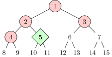
(a) BFS

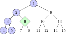
(b) DFS

Figure 1: The difference between BFS (left) and DFS (right) in a complete binary tree where a goal (diamond) is placed in the second position on level 2 (the third row). The numbers indicate traversal order. Circled nodes are explored before the goal is found. Note how BFS and DFS explore different parts of the tree. In bigger trees, this may lead to substantial differences in search performance.

Tree search and graph search

BFS and DFS come in two flavors, depending on whether they keep track of visited nodes or not. The tree search variants do not keep track of visited nodes, while the graph search variants do. In trees (where each node can only be reached through one path), nothing is gained by keeping track of visited nodes. In contrast, keeping track of visited nodes can benefit search performance greatly in multiply connected graphs, although especially for DFS the additional memory consumption may sometimes be prohibitive. Algorithm 1 describes BFS tree search and graph search. DFS tree search (Algorithm 2) is substantially more memory-efficient than DFS graph search (Algorithm 2) and BFS: $O(d)$ compared to $O(b^{d})$. However, BFS can be emulated by iterative deepening DFS (ID-DFS). ID-DFS uses the same amount of memory as DFS tree search, and only has a slightly longer runtime than BFS in most graphs (Russell and Norvig,, 2010, Sec. 3.4.5).

For general graphs, we consider DFS with bounded search depth. Without a bound, a single path may span the entire or a very large portion of the search space, giving the search more the characteristics of a random walk than of search with backtrack. An unbounded DFS tree search may require as much memory as a BFS search. This justifies the study of depth-bounded DFS tree search (Algorithm 2). A depth-bounded DFS graph search may be analysed with almost the same method, and is interesting for comparison. Unfortunately, depth-bounded DFS graph search is not a complete search method in general graphs, as the search might cut itself off from regions of the search space. (See Figure 2 for an example.) In trees, the search strategies of DFS tree search and DFS graph search are indistinguishable.

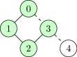
Figure 2: Depth-bounded DFS graph search with radius 3 cutting itself off from node 4. After node 3 has been visited, the search backtracks to the root node 0. While node 4 could originally have been visited via 0–3–4, this path is now blocked since node 3 already has been visited. DFS tree search does not have this problem.

3.3 Algorithm performance

Performance on a single problem may be defined in terms of:

1. Solution quality.

2. The number of explored states (a state $s$ is explored if either $N(s)$ or $C(s)$ has been called).

3. The running time of the algorithm.

4. The memory consumption of the algorithm (typically measured by the maximum number of states kept in memory).

(Asymptotic) average or worst-case analysis may be used when measuring performance on a class of problems.

In this work, we will measure performance by the average number of explored states until a goal is found; that is, item 2 and assuming only the first satisfactory goal matters. In many cases the number of explored states is proportional to the actual runtime (item 3), since state expansion often is the dominant operation during search. We therefore permit ourselves to refer to the number of nodes explored until a first goal is found as the runtime or search time. For example, the runtime of BFS is 5 and the runtime of DFS is 6 in Figure 1. If no goal exists, the search method will explore all nodes before halting. In this case, we define the runtime as the number of nodes in the search problem plus 1 (i.e., $2^{D+1}$ in the case of a binary tree of depth $D$).

3.4 Probability Theory

The random variables $X_{1},\dots,X_{n}$ are independent and identically distributed (iid) if for all $i\in\{1,\dots,n\}$ and any outcome $x$, $P(X_{i}\leq x)=P(X_{1}\leq x)$, and the probability of any joint outcome $x_{1},\dots,x_{n}$ satisfies $P(X_{1}\leq x_{1},\dots,X_{n}\leq x_{n})=\prod_{i=1}^{n}P(X_{i}\leq x_{i})$.

A random variable $X$ is geometrically distributed $\mathrm{Geo}(p)$ if $P(X=k)=(1-p)^{k-1}p$ for $k\in\{1,2,\dots\}$. The interpretation of $X$ is the number of trials until the first success when each trial succeeds with iid probability $p$. Its cumulative distribution function (CDF) is $P(X\leq k)=1-(1-p)^{k}$, and its average or expected value is $\mathbb{E}[X]=1/p$. When success is guaranteed to occur within the first $m$ trials, a truncated geometric distribution arises. A random variable $Y$ is truncated geometrically distributed $X\sim\mathrm{TruncGeo}(p,m)$ if $Y=(X\mid X\leq m)$ for $X\sim\mathrm{Geo}(p)$, which gives

$$P(Y=k) =\begin{cases}\frac{(1-p)^{k}p}{1-(1-p)^{m}}&\text{for }k\in\{1,\dots,m\}\\ 0&\text{otherwise.}\end{cases}$$

$$\mathbb{E}[Y]=\mathrm{tc}(p,m) =\mathbb{E}[X\mid X\leq m]=\frac{1-(1-p)^{m}(pm+1)}{p(1-(1-p)^{m})}.$$

When $p\gg\frac{1}{m}$, $Y$ is approximately $\mathrm{Geo}(p)$, and $\mathrm{tc}(p,m)\approx\frac{1}{p}$. When $p\ll\frac{1}{m}$, $Y$ becomes approximately uniform on $\{1,\dots,m\}$ and $\mathrm{tc}(p,m)\approx\frac{m}{2}$.

A random variable $Z$ is exponentially distributed $\mathrm{Exp}(\lambda)$ if $P(Z\leq z)=1-e^{-\lambda z}$ for $z\geq 0$. The expected value of $Z$ is $1/\lambda$, and the probability density function of $Z$ is $\lambda e^{-\lambda z}$. An exponential distribution with parameter $\lambda=-\ln(1-p)$ can be viewed as the continuous counterpart of a $\mathrm{Geo}(p)$ distribution. We will use this approximation in Section 5.

Lemma 3 (Exponential approximation).

Let $Z\sim\mathrm{Exp}(-\ln(1-p))$ and $X\sim\mathrm{Geo}(p)$. Then the CDFs for $X$ and $Z$ agree for integers $k$, $P(Z\leq k)=P(X\leq k)$. The expectations of $Z$ and $X$ are also similar in the sense that $0\leq\mathbb{E}[X]-\mathbb{E}[Z]\leq 1$.

Proof.

For $z>0$, $P(Z\leq z)=1-\exp(z\ln(1-p))=1-(1-p)^{z}$, and $P(X\leq z)=1-(1-p)^{\lfloor z\rfloor}$. Thus, for integers $k>0$, $P(Z\leq k)=P(X\leq k)$ which proves the first statement. Further, $1-(1-p)^{\lfloor z\rfloor}\leq 1-(1-p)^{z}<1-(1-p)^{\lfloor z+1\rfloor}$, so $P(X\leq z)\leq P(Z\leq z)<P(X-1\leq z)$. Hence $\mathbb{E}[X]\geq\mathbb{E}[Z]>E[X-1]=\mathbb{E}[X]-1$, which proves the second statement. ∎

We will occasionally make use of the convention $0\cdot\mathit{undefined}=0$.

Let $\Omega$ be a sample space, i.e. a set of possible outcomes. The Law of Total Expectation allows us to expand expectations by conditioning on disjoint events:

Lemma 4.

Let $X$ be a random variable and let the sample space $\Omega=\dot{\bigcup}_{i\in I}C_{i}$ be partitioned by mutually disjoint events $C_{i}$. Then $\mathbb{E}[X]=\mathbb{E}[\mathbb{E}[X\mid C_{i}]]=\sum_{i\in I}P(C_{i})E[X\mid C_{i}]$.

This concludes the background section, and the stage is now set for the analysis proper.

4 Tree with a Single Goal Level

We start with analysing expected BFS and DFS runtime in trees. The results apply when the search graph is a tree, and when tree search versions of BFS and DFS are used (in which case any graph “looks like” a tree, as discussed in Section 3.2). This section assumes that all goals are located on a single level of the tree; i.e., all goals have the same distance from the start node. This is usually unrealistic, but makes the analysis easier. The next section relaxes the assumption of a single goal level.

Our aim throughout is to derive closed-form approximations for BFS and DFS expected search time. Figure 1 illustrates the different search strategies BFS and DFS, and how they initially focus the search on different areas of the tree: BFS stays close to the root while DFS goes directly to the bottom. In this section only, the comparison between BFS and DFS expected search time yields an elegant decision boundary between which method is better in expectation.

As a concrete example, consider the problem of solving a Rubik’s cube. Rokicki and Kociemba, (2013) did a thorough analysis of this problem, and found that there is an upper bound to how many moves it can take to reach the goal, and that most goals are located around level 17 ($\pm 2$ levels). If we consider search algorithms that do not remember where they have been, the search space becomes a complete tree with fixed branching factor 18 (or 13.3 on average, if we cannot immediately return to the preceding state) (Edelkamp and Korf,, 1998). What would be the expected BFS and DFS search time for this problem? Which one would be faster?

The model

Our single goal level model is defined by the following and illustrated in Figure 3. In a binary tree of depth $D$, let solutions be distributed on a single goal level $g\in\{0,\dots,D\}$. At the goal level, any node is a goal with iid probability $p_{g}\in[0,1]$. We will refer to these kinds of problems as (single goal level) complete binary trees with depth $D$, goal level $g$ and goal probability $p_{g}$.

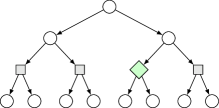
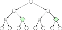
Figure 3: Two possible outcomes of goal distribution in a single goal level problem with max depth $D=3$, goal level $g=2$ (boxes) with nodes being goals (diamonds) with iid probability $p_{g}=1/3$. Depending on goal locations, BFS and DFS performance will differ. We are interested in expected performance.

Note that there may be several or zero goals. Denote with $\Gamma$ the event that a goal exists, and $\overline{\Gamma}$ the event that no goal exists. It will be useful later to also define $\Gamma_{k}$ as the event that a goal exists on level $k$, and $\overline{\Gamma}_{k}$ as its complement. The probability that a goal exists is $P(\Gamma)=P(\Gamma_{g})=1-(1-p_{g})^{2^{g}}$. If a goal exists, let $Y\in\{1,\dots,2^{g}\}$ be the position of the first goal at level $g$. Conditioned on a goal existing, $Y$ is a truncated geometric variable $Y\sim\mathrm{TruncGeo}(p_{g},2^{g})$. When $p_{g}\gg 2^{-g}$ the goal position $Y$ is approximately $\mathrm{Geo}(p_{g})$, which makes most expressions slightly more elegant. This is often a realistic assumption since we usually expect the problem to have a solution. If $p\not\gg 2^{-g}$, then the likelihood of no goal is large. Our analysis does not require that a goal exists.

Runtime estimates

The following two propositions give runtime estimates for BFS and DFS by following the counting schemes illustrated in Figure 4. The BFS result is particularly simple. Throughout the paper, we use $t^{\mathit{alg}}_{{\textit{problem type}}}$ to denote expected search time for algorithm alg on the subscripted problem type. A tilde on top denotes rough approximation.

Proposition 5 (BFS runtime Single Goal Level).

Let the problem be a complete binary tree with depth $D$, goal level $g$ and goal probability $p_{g}$. When a goal exists and has position $Y$ on the goal level, the BFS search time is

$$t^{\mathrm{BFS}}_{\mathrm{SGL}}(g,p_{g},Y) =2^{g}-1+Y\text{, with expectation}$$ (1)

$$t^{\mathrm{BFS}}_{\mathrm{SGL}}(g,p_{g}\mid\Gamma_{g}) =2^{g}-1+\mathrm{tc}(p_{g},2^{g})\approx 2^{g}-1+\frac{1}{p_{g}}.$$ (2)

In general, when a goal does not necessarily exist, the expected BFS search time is

$$t^{\mathrm{BFS}}_{\mathrm{SGL}}(g,p_{g})=P(\Gamma)\cdot(2^{g}-1+\mathrm{tc}(p_{g},2^{g}))+P(\overline{\Gamma})\cdot 2^{D+1}\approx 2^{g}-1+\frac{1}{p_{g}}.$$ (3)

The right hand approximations of (2) and (3) are close when $p_{g}\gg 2^{-g}$ and $D\not\gg g$.

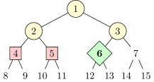
(a) BFS count

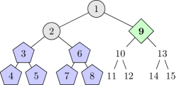
(b) DFS count

Figure 4: The counting schemes used in Propositions 6 and 5, illustrated in a tree of depth 3. The BFS count is illustrated with a goal (diamond) on the third position on level 2, while the DFS count is illustrated with a goal on level 2.

Proof.

When a goal exists, BFS will first explore all of the top of the tree until depth $g-1$: The $2^{(g-1)+1}=2^{g}$ nodes that are circles in Figure 4(a). BFS will then search $Y$ nodes on level $g$ (boxes and diamond in Figure 4(a)). The total search time is thus $t^{\mathrm{BFS}}_{\mathrm{SGL}}(D,g,p_{g},Y)=2^{g}-1+Y$, with expected value $2^{g}-1+\mathrm{tc}(p_{g},2^{g})$.

In the general case when a goal does not necessarily exist, the expected value of the search time $X$ expands as

$$\mathbb{E}[X] =P(\Gamma)\cdot\mathbb{E}[X\mid\Gamma]+P(\overline{\Gamma})\cdot\mathbb{E}[X\mid\overline{\Gamma}]$$

$$=P(\Gamma)\cdot t^{\mathrm{BFS}}_{\mathrm{SGL}}(D,p,p_{g}\mid\Gamma_{g})+P(\overline{\Gamma})\cdot 2^{D+1}$$

$$=P(\Gamma)\cdot(2^{g}-1+\mathrm{tc}(p_{g},2^{g}))+P(\overline{\Gamma})\cdot 2^{D+1}.$$

When $p_{g}\gg 2^{-g}$, then $Y\approx\mathrm{Geo}(p)$, and $P(\Gamma)\approx 1$ and $P(\overline{\Gamma})\approx 0$. Further, $2^{D}\not\gg 2^{g}$ since $D\not\gg g$, so the term $P(\overline{\Gamma})2^{D}$ cannot significantly affect the expectation. This justifies the $(1/p_{g}-1)2^{D-g+1}$ approximation. ∎

Proposition 5 can be compared with the more general result for IDA* by Korf et al., (2001). A memory-efficient tree-search variant of BFS can be implemented as iterative deepening DFS (ID-DFS). The runtime of ID-DFS is about twice the runtime of BFS. Korf et al.,’s bound comes out as $t^{\mathrm{BFS}}_{\mathrm{SGL}}(g)\approx 2^{g+2}$, which corresponds to a doubling of the worst case of $Y=2^{g}$ in (1). The doubling is correct since ID-DFS is twice as slow as BFS in the worst case.

We next turn to analyse DFS in a similar manner.

Proposition 6 (DFS runtime Single Goal Level).

Consider a complete binary tree with depth $D$, goal level $g$ and goal probability $p_{g}$. When a goal exists and has position $Y$ on the goal level, the DFS search time is approximately

$$\tilde{t}^{\mathrm{DFS}}_{\mathrm{SGL}}(D,g,p_{g},Y) :=(Y-1)2^{D-g+1}+2\text{, with expectation}$$

$$\tilde{t}^{\mathrm{DFS}}_{\mathrm{SGL}}(D,g,p_{g}\mid\Gamma_{g}) :=\left(\mathrm{tc}(p_{g},2^{g})-1\right)2^{D-g+1}+2\approx\left(\frac{1}{p_{g}}-1\right)2^{D-g+1}+2.$$ (4)

The expected DFS search time when a goal does not necessarily exist is approximately

$$\tilde{t}^{\mathrm{DFS}}_{\mathrm{SGL}}(D,g,p_{g}):=P(\Gamma)((\mathrm{tc}(p_{g},2^{g})-1)2^{D-g+1}+2)+P(\overline{\Gamma})2^{D+1}\!\approx\!\!\left(\frac{1}{p_{g}}\!-\!1\!\right)\!2^{D-g+1}\!\!.$$ (5)

The right hand approximations in (4) and (5) are valid when $p_{g}\gg 2^{-g}$.

Proof.

One way to count the nodes explored by DFS when a goal exists is the following. To the left of the first goal on level $g$, DFS will explore $2(Y-1)$ subtrees rooted at level $g+1$ (pentagons in Figure 4(b)). These subtrees will have depth $D-(g+1)$, and contain $2^{D-g}-1$ nodes each. DFS will also explore $Y$ nodes on level $g$ and their parents, which amounts to about $2Y$ nodes (circles in Figure 4(b)). Summing the contributions gives the DFS search time approximation $\tilde{t}^{\mathrm{DFS}}_{\mathrm{SGL}}(D,g,p_{g},Y)=2(Y-1)\cdot(2^{D-g}-1)+2Y=(Y-1)2^{D-g+1}+2$.

By Lemma 4, the expected value of the search time $X$ when a goal does not necessarily exist expands as

$$\mathbb{E}[X] =P(\Gamma)\cdot\mathbb{E}[X\mid\Gamma]+P(\overline{\Gamma})\cdot\mathbb{E}[X\mid\overline{\Gamma}]$$

$$=P(\Gamma)\cdot\mathbb{E}[\tilde{t}^{\mathrm{DFS}}_{\mathrm{SGL}}(D,g,p_{g},Y)\mid\Gamma]+P(\overline{\Gamma})\cdot 2^{D+1}$$

$$=P(\Gamma)\cdot((\mathrm{tc}(p_{g},2^{g})-1)2^{D-g+1}+2)+P(\overline{\Gamma})\cdot 2^{D+1}$$

where the last step uses that $(Y\mid\Gamma)\sim\mathrm{TruncGeo}(p_{g},2^{g})$. When $p_{g}\gg 2^{-g}$, then $\Gamma\approx 1$, $\overline{\Gamma}\approx 0$ and $Y\approx\mathrm{Geo}(p_{g})$ which justifies the approximation. ∎

Propositions 6 and 5 provide expected runtime estimates as a function of the parameters $D$, $g$, and $p_{g}$. Figure 11 in Section 9 plots the runtime estimates as functions of the goal level $g$. As expected, one observation that can be made from these results is that BFS benefits when goals are close to the start node, and DFS benefits when goals are close to the maximum search depth of the tree. This can be seen from positive $g$ exponent in Proposition 5 for BFS, and the negative $g$ exponent in Proposition 6 for DFS. The runtimes are also plotted as a function of $g$ in Figure 11. Although the model is unrealistic, these results provide important building blocks for the more general models in subsequent sections.

Decision boundary

An interesting point to analyse is the crossover where DFS overtakes BFS in performance. This crossover occurs where the difference $t^{\mathrm{BFS}}_{\mathrm{SGL}}-\tilde{t}^{\mathrm{DFS}}_{\mathrm{SGL}}$ between BFS and DFS runtimes shifts sign. It turns out that this crossover has an elegant expression:

Proposition 7 (Decision boundary for single goal level binary tree).

Let $\gamma_{p_{g}}=\log_{2}\left(\mathrm{tc}(p_{g},2^{g})-1\right)/2\approx\log_{2}\left(\frac{1-p_{g}}{p_{g}}\right)/2$. Given the approximation of DFS runtime of Proposition 6, BFS wins in expectation in a complete binary tree with depth $D$, goal level $g$ and goal probability $p_{g}$ when

$$g<\frac{D}{2}+\gamma_{p_{g}}$$

and DFS wins in expectation when $g>\frac{D}{2}+\gamma_{p_{g}}+\frac{1}{2}$.

The approximation $\gamma_{p_{g}}\approx\log_{2}\left(\frac{1-p_{g}}{p_{g}}\right)/2$ is valid when $p_{g}\gg 2^{-g}$. The proposition holds regardless of this assumption.

Proof.

When no goal exists, BFS and DFS will perform the same. When the tree contains at least one goal node, BFS will find the goal somewhere on its sweep across level $g$, so the BFS runtime is bounded between $2^{g}\leq t^{\mathrm{BFS}}_{\mathrm{SGL}}(g,p_{g})\leq 2^{g+1}$.

The upper bound for $t^{\mathrm{BFS}}_{\mathrm{SGL}}(g,p_{g})$ gives that $t^{\mathrm{BFS}}_{\mathrm{SGL}}(g,p_{g})<t_{\mathrm{DFS}}(D,g,p_{g})$ when $2^{g+1}<\left(\mathrm{tc}(p_{g},2^{g})-1\right)2^{D-g+1}$. Taking the binary logarithm of both sides yields

$$g+1 <\log_{2}\left(\mathrm{tc}(p_{g},2^{g})-1\right)+D-g+1.$$

Collecting the $$g$$’s on one side and dividing by 2 gives the desired bound

$$g <\frac{\log_{2}(\mathrm{tc}(p_{g},2^{g})-1)}{2}+\frac{D}{2}=\frac{D}{2}+\gamma_{p_{g}}.$$

Similar calculations with the lower bound for $t^{\mathrm{BFS}}_{\mathrm{SGL}}(g,p_{g})$ gives the condition for $\tilde{t}^{\mathrm{DFS}}_{\mathrm{SGL}}(D,g,p_{g})<t^{\mathrm{BFS}}_{\mathrm{SGL}}(g,p_{g})$ when $g>\frac{D}{2}+\gamma_{p_{g}}+\frac{1}{2}$. ∎

The term $\gamma_{p_{g}}$ is in the range $[-1,1]$ when $p_{g}\in[0.2,0.75]$, $g\geq 2$, in which case Proposition 7 roughly says that BFS wins (in expectation) when the goal level $g$ is located higher than the middle of the tree. That the decision boundary is halfway between top and bottom is somewhat surprising given the different natures of the explored areas of BFS and DFS. While BFS exhaustively explores one subtree at the top, DFS typically exhaustively explores several lower subtrees next to the bottom (see Figure 4). Note that the goal probability $p_{g}$ needs to be quite large for this balance to occur.

For smaller, more realistic $p_{g}$, BFS benefits with the boundary being shifted $\gamma_{p_{g}}\approx k$ levels from the middle for $p_{g}\approx 2^{-2k}$. In other words, DFS benefits to a greater degree than BFS from a high goal probability. The reason is that when the goal probability is very high, the best search strategy is to follow an arbitrary path down the tree. With high probability the path will hit a goal. When the goal probability is smaller, substantial backtracking will be required. Figure 12 on page 12 illustrates the decision boundary as a function of goal depth and tree depth for a fixed probability $p_{g}=0.07$, and shows that Proposition 7 can be used to accurately predict whether BFS or DFS will be faster.

It is straightforward to generalise the calculations to arbitrary branching factor $b$ by substituting the 2 in the base of $t^{\mathrm{BFS}}_{\mathrm{SGL}}$ and $\tilde{t}^{\mathrm{DFS}}_{\mathrm{SGL}}$ for $b$. In Proposition 7, the change only affects the base of the logarithm in $\gamma_{p_{g}}$:

Corollary 8 (Decision boundary general).

Given the above approximations to BFS and DFS runtime, BFS wins in expectation in a complete tree with integer branching factor $b\geq 2$, depth $D$, goal level $g$, and goal probability $p_{g}$ when $g<\frac{D}{2}+\gamma_{b,p_{g}}$, and DFS wins in expectation when $g>\frac{D}{2}+\gamma_{b,p_{g}}+\frac{1}{2}$, where $\gamma_{b,p_{g}}=\log_{b}\left(\mathrm{tc}(p_{g},b^{g})-1\right)/2\approx\log_{b}(\frac{1-p_{g}}{p_{g}})/2$.

The approximation $\gamma_{b,p_{g}}\approx\log_{2}\left(\frac{1-p_{g}}{p_{g}}\right)/2$ is valid when $p_{g}\gg b^{-g}$, but the result does not otherwise depend on this assumption. The clean results obtained in this section are encouraging. The next section relaxes the arguably unrealistic assumption of a single goal level.

5 Tree with Multiple Goal Levels

We now generalise the model developed in the previous section to problems that can have goals on any number of levels. Approximate expected runtime results are obtained for both BFS and DFS. The BFS analysis is a straightforward generalisation of the techniques in the previous section. The DFS analysis requires a bit more work and an additional approximation of the distribution of the position of the first goal on a level.

The model is the following. For each level $k\in\{0,\dots,D\}$, let $p_{k}$ be the associated goal probability. Not every $p_{k}$ should be equal to 0. Nodes are goals or not independently of each other. Nodes on level $k$ have probability $p_{k}$ of being goals. Let $Y_{k}$ be the position of the first goal on level $k$ if such a goal exists. We will refer to these kinds of problems as (multi goal level) complete binary trees with depth $D$ and goal probabilities ${\mathbf{p}}=[p_{0},\dots,p_{D}]$. An example is depicted in Figure 5.

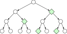
Figure 5: Tree with Multiple Goal Levels model of depth $D=3$ and goal generated from the goal probability vector ${\mathbf{p}}=[0,\frac{1}{3},\frac{1}{3},\frac{1}{3}]$

Permitting goals on any level with different probability for each level makes the model significantly more realistic, as in most cases goals are not located on a single goal level. A major open question that remains is how to estimate the goal probability vector in practice. We discuss this further in Section 11.

Notation

Let $\Gamma_{i}$ be the event that level $i$ has a goal, with $P(\Gamma_{i})=1-(1-p_{i})^{2^{i}}$. As before, let $\Gamma=\bigcup_{i}\Gamma_{i}$ be the event that a goal exists, and let $\overline{\Gamma}$ and $\overline{\Gamma}_{i}$ be their complements.

5.1 DFS Analysis

To find an approximation of goal DFS expected runtime in trees with multiple goal levels, we approximate the geometric distribution used in Proposition 6 with an exponential distribution (its continuous approximation by Lemma 3).

Proposition 9 (DFS runtime for multiple goal levels).

Consider a complete binary tree of depth $D$ with goal probabilities ${\mathbf{p}}=[p_{0},\dots,p_{D}]\in[0,1)^{D+1}$. If for all $k$, $p_{k}\ll 1$ and $Y_{k}\sim\mathrm{Geo}(p_{k})$, then the expected number of nodes DFS will search is approximately

$$\tilde{t}^{\mathrm{DFS}}_{\mathrm{MGL}}(D,{\mathbf{p}}):=P(\Gamma)/\sum_{k=0}^{D}\ln(1-p_{k})^{-1}2^{-(D-k+1)}+P(\overline{\Gamma})2^{D+1}.$$

The assumption $Y_{k}\sim\mathrm{Geo}(p_{k})$ is approximately true when $p_{k}\gg 2^{-k}$. If some level $k$ has a smaller $p_{k}$, then the probability that the search encounters a goal at this level is small. Thus, we expect the result to be approximately true even if $Y_{k}\sim\mathrm{Geo}(p_{k})$ only for some levels. Empirical results in Section 9 verify the validity of the approximations.

The proof constructs for each level $k$ an exponential random variable $X_{k}$ that approximates the search time before a goal is found on level $k$ (disregarding goals on other levels). The minimum of all $X_{k}$ then becomes an approximation of the search time to find a goal on some level. The approximations use exponential variables for easy minimisation.

Proof of Proposition 9.

The second term $P(\overline{\Gamma})2^{D+1}$ covers the case of no goal being present, and follows immediately from Lemma 4 and the search time being $2^{D+1}$ when no goal exists.

For the more interesting case of a goal existing, the proof uses two approximations. First approximate the position of the first goal on level $k$ with $Y_{k}\approx\mathrm{Exp}(\lambda_{k})$, where $\lambda_{k}=-\ln(1-p_{k})$. The approximation is justifiable by Lemma 3, since we assumed $Y_{k}\sim\mathrm{Geo}(p_{k})$.

Second, disregarding goals on levels other than $k$, the total number of nodes that DFS needs to search before reaching a goal on level $k$ is approximately $X_{k}\sim\mathrm{Exp}(\lambda_{k}2^{-(D-k+1)})$. This follows from an approximation of Proposition 6: The number of nodes DFS needs to search to find a goal on level $k$ is

$$\tilde{t}^{\mathrm{DFS}}_{\mathrm{SGL}}(D,k,p_{k},Y_{k})=(Y_{k}-1)2^{D-k+1}+2\approx Y_{k}\cdot 2^{D-k+1}.$$

(This is a reasonable estimate if $Y_{k}$ is large, which is likely given that $p_{k}\ll 1$ by assumption.) So $X_{k}$ is approximately a multiple $2^{D-k+1}$ of $Y_{k}$. For any exponential random variable $Z$ with parameter $\lambda$, the scaled variable $m\cdot Z$ is $\mathrm{Exp}(\lambda/m)$. This completes the justification of the second approximation.

The result now follows by a standard minimisation of exponential variables. Since $X_{k}$ is the number of nodes searched before finding a goal on level $k$, the number of nodes searched before finding a goal on any level is $X=\min_{k}X_{k}$. The CDF for $X$ is approximately

$$P(X\leq y) =1-\prod_{k=0}^{D}P(X_{k}>y)$$

$$=1-\prod_{k=0}^{D}\exp(-\lambda_{k}2^{-(D-k+1)}y)$$

$$=1-\exp(-y\sum_{k=0}^{D}\lambda_{k}2^{-(D-k+1)}).$$

(The minimum of exponential variables $Z_{k}\sim\mathrm{Exp}(\xi_{k})$ is again an exponential variable $\mathrm{Exp}(\sum\xi_{k})$.)

Thus the search time when a goal exists is $X\sim\mathrm{Exp}(\sum_{k=0}^{D}\lambda_{k}2^{-(D-k+1)}))$, so the expected search time is $1/\sum_{k=0}^{D}\lambda_{k}2^{-(D-k+1)})$. This completes the analysis of the case where a goal exists. Finally multiplying with the probability $P(\Gamma)$ that a goal exists justifies the first term in the approximation (compare Lemma 4). ∎

In the special case of a single goal level $j$ with $p_{j}\gg 2^{-j}$, the result of Proposition 9 is similar to the approximation in Proposition 6. When ${\mathbf{p}}$ only has a single element $p_{j}\not=0$ and $p_{j}\gg 2^{-j}$, the expression $\tilde{t}^{\mathrm{DFS}}_{\mathrm{MGL}}$ simplifies to

$$\tilde{t}^{\mathrm{DFS}}_{\mathrm{MGL}}(D,{\mathbf{p}})=P(\Gamma)\frac{1}{\lambda_{j}}2^{D-j+1}+P(\overline{\Gamma})2^{D+1}\approx\frac{1}{\lambda_{j}}2^{D-j+1}=-\frac{1}{\ln(1-p_{j})}2^{D-j+1}.$$

For $p_{j}$ not close to 1, the factor $-1/\ln(1-p_{j})$ is approximately the same as the corresponding factor $1/p_{j}-1$ in Proposition 6 (the Laurent expansion is $-1/\ln(1-p_{j})=1/p_{j}-1/2+O(p_{j})$).

The DFS runtime result can be adapted to the case where at least one goal must be present. Simply replace $P(\Gamma)$ with 1, and remove the second term $P(\overline{\Gamma})2^{D+1}$.

5.2 BFS Analysis

The corresponding expected search time $t^{\mathrm{BFS}}_{\mathrm{MGL}}(D,{\mathbf{p}})$ for BFS requires less insight and can be calculated exactly by conditioning on which level the first goal is. The resulting formula is less elegant, however. The same technique cannot be used for DFS, since DFS does not exhaust levels one by one.

To develop the reduction to the single goal level case, some extra notation needs to be introduced. Let $F_{k}=\Gamma_{k}\cap(\bigcap_{i=0}^{k-1}\overline{\Gamma}_{i})$ be the event that level $k$ has the first goal. The probability that level $k$ has the first goal is $P(F_{k})=P(\Gamma_{k})\prod_{j=0}^{k-1}P(\overline{\Gamma}_{j})$. The expected BFS search time gets a more uniform expression by the introduction of an extra hypothetical level $D+1$ where all nodes are goals. That is, regardless of the goal probabilities of the problem, we assume that level $D+1$ has goal probability $p_{D+1}=1$ and $P(F_{D+1})=P(\overline{\Gamma})=1-\sum_{k=0}^{D}P(F_{k})$.

Proposition 10 (BFS runtime for multiple goal levels).

The expected number of nodes $t^{\mathrm{BFS}}_{\mathrm{MGL}}(p)$ that BFS needs to search to find a goal in a complete binary tree of depth $D$ with goal probabilities ${\mathbf{p}}=[p_{0},\dots,p_{D}]$, is

$$t^{\mathrm{BFS}}_{\mathrm{MGL}}({\mathbf{p}})=\sum_{k=0}^{D+1}P(F_{k})t^{\mathrm{BFS}}_{\mathrm{SGL}}(k,p_{k}\mid\Gamma_{k})\approx\sum_{k=0}^{D+1}P(F_{k})\left(2^{k}+\frac{1}{p_{k}}\right)$$

For $p_{k}=0$, the expression $t^{\mathrm{BFS}}_{\mathrm{CB}}(k,p_{k})$ and $1/p_{k}$ will be undefined, but this only occurs when $P(F_{k})$ is also 0. The BFS runtime estimate can easily be modified to the situation where at least one goal must exist. Simply drop the $(D+1)$st term in the sum, and renormalise the probabilities $P(F_{0}),\dots,P(F_{D})$.

Proof.

To BFS, the event $F_{k}$ that level $k$ has a goal is equivalent to the single goal level model of Section 4. Let $X$ be BFS search time, and let $(X\mid F_{k})$ be the number of nodes that BFS needs to search when $k$ is the first level with a goal. Then $(X\mid F_{k})=t^{\mathrm{BFS}}_{\mathrm{SGL}}(k,p_{k},X-(2^{k}-1)\mid\Gamma_{k})$, and $\mathbb{E}[X\mid F_{k}]=t^{\mathrm{BFS}}_{\mathrm{SGL}}(k,p_{k}\mid\Gamma_{k})$. The result follows by expanding $\mathbb{E}[X]$ over $F_{0},\dots,F_{D+1}$ as in Lemma 4. ∎

The approximation $\sum_{k=0}^{D+1}P(F_{k})\left(2^{k}+\frac{1}{p_{k}}\right)$ tends to be within a factor 2 of the correct expression, even when $p_{k}<2^{-k}$ for some or all $p_{k}\in{\mathbf{p}}$. The reason is that the corresponding $P(F_{k})$’s are small when the geometric approximation is inaccurate.

Discussion

Propositions 9 and 10 provide closed-form approximations for expected runtime of DFS and BFS in graphs with goals on any number of levels and with essentially any combination of goal probabilities. Given knowledge of the goal probabilities, expected BFS and DFS search time can easily be computed. Such knowledge is useful when estimating the amount of resources that will be required to solve a problem, and when deciding whether the problem is approachable at all. Expected runtime is often more relevant than worst case runtime, as most realistic problems may be significantly easier than the worst ones.

We have not managed to derive a similarly elegant closed-form decision boundary as for the single goal level case (Proposition 7). However, a simple computer program can still easily compare the runtime estimates of Propositions 9 and 10 for a given goal probability vector. The comparison can be used to predict the BFS vs. DFS winner. The decision boundary from this prediction is plotted for a concrete set of goal probability vectors in Figure 12.

The open question of estimating the goal probability vector is discussed further in Section 11. Both Propositions 9 and 10 naturally generalise to arbitrary branching factor $b$.

6 Graph Search

In this section, we explore general graphs. In addition to analysing the performance of graph search BFS and DFS (that do remember visited nodes) we also analyse the performance of tree search DFS in general graphs. Graph search can significantly improve performance, but in return requires more memory. For DFS, the difference is exponential; for BFS only minor. Figure 6 gives an idea of BFS and DFS graph search behaviour.

The model

General, non-tree graphs exhibit significantly more variability than trees. Graphs vary along dimensions such as connectivity and path-redundancy, as well as average number of neighbours. We capture this variability in what we call a length-to-depth counter $L$:

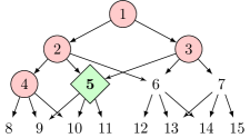
(a) BFS

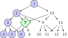
(b) DFS

Figure 6: The difference between BFS and DFS in multiply connected graphs. Note how DFS is additionally concentrated at the bottom of the graph compared to Figure 1.

Definition 11 (Distance, level, and length-to-depth counter).

Let the distance $\mathrm{dist}(u,v)$ be the shortest path between $u$ and $v$. Let the level of a node $v$, $\mathrm{level}(v)=\mathrm{dist}(v_{0},v)$, be the distance from the start node to $v$. Let $D=\max_{v}\mathrm{level}(v)$ be the maximum depth, and let $D^{\prime}$ be the radius of search for DFS. Let $\delta_{n}$ be the first node to which DFS has travelled $n$ steps, $0\leq n\leq D^{\prime}$.

The level-to-depth counter $L$ plays a central role in the analysis. For a given search problem, let

$$L(n,d)=\mathbb{E}\big{[}|\{v:\mathrm{level}(v)=d,\mathrm{dist}(\delta_{n},v)<D^{\prime}-n\}|\big{]}$$

be the expected number of nodes on level $d$ reachable from $\delta_{n}$ within the remaining path length $D^{\prime}-n$. Let $\overline{L}(n,d)$ be the same quantity, but with nodes counted with repetition if they can be reached through multiple paths.

For example, if $D^{\prime}=2$ then $L(1,2)$ is the expected number of neighbours on level 2 after having taken the first search step. The length-to-depth counter plays the role of a sufficient statistic for search time for graphs. Although many different graphs have identical length-to-depth counters, our results below imply that any two graphs with identical length-to-depth counters will have the same expected search time. In many graphs, the length-to-depth counter can be connected to the branching factor (Section 7). As in the previous section, we assume that goals are distributed by level in an iid manner according to a goal probability vector ${\mathbf{p}}$. We will also assume that the probability of DFS finding a goal before finding $\delta_{D}$ is negligible. We will refer to these kinds of problems as search problems with depth $D$, goal probabilities ${\mathbf{p}}$ and level-to-depth counter $L$. The rest of this section justifies the following proposition.

Proposition 12.

The DFS and BFS runtime of a search problem can be roughly estimated from the level-to-depth counters $L$ and $\overline{L}$, the depth $D$, and the goal probabilities ${\mathbf{p}}=[p_{0},\dots,p_{D}]$ when the probability of finding a goal before $\delta_{D}$ is negligible.

The assumption of DFS having a negligible probability of finding a goal before $\delta_{D}$ is satisfied in problems where

• nodes typically have several neighbours, so that premature backtracking before the full radius is reached usually is not necessary, and

• no level $k$ has goal probability $p_{k}$ close to 1.

These assumptions are satisfied in a wide range of practical problems, including most of the instances investigated in Section 9.

6.1 DFS Analysis

We analyse both DFS tree search and DFS graph search (Algorithms 2 and 3 on Algorithms 2 and 3 above). Although the analysis in Sections 4 and 5 can be used to analyse DFS tree search in graphs, such an analysis would require an interpretation of level as path length (as interpreted in Algorithm 2) rather than shortest distance. The analysis performed in this section compares nicely with the corresponding BFS analysis.

Sets of nodes

Recall that $\delta_{n}$ is the first node to which DFS has travelled $n$ steps, and that $D^{\prime}$ is the radius of search for DFS. Unless DFS has been forced to backtrack, $\delta_{n}$ will be the $n$th node expanded. We will assume that $\delta_{D^{\prime}}$ is reached in roughly $D^{\prime}$ steps. The nodes $\delta_{0},\dots,\delta_{D^{\prime}}$ play a central role in the analysis, since the descendants of $\delta_{n+1}$ will be explored before the descendants of $\delta_{n}$ (possibly excluding the $\delta_{n+1}$ descendants). We say that DFS explores from $\delta_{n}$ after DFS has explored all descendants of $\delta_{n+1}$ and until all descendants of $\delta_{n}$ have been explored. The general idea of the DFS analysis will be to count the number of nodes under each $\delta_{n}$, and to compute the probability that any of these nodes is a goal.

Some notation for this (see Figure 7 for illustration):

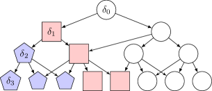
Figure 7: The notation for the DFS graph analysis. Each node $\delta_{n}$ is the first node explored by DFS on level $n$. Pentagons denote the $\delta_{2}$ subgraph $S_{2}$, and boxes the $\delta_{1}$ explorables $T_{1}$. The length-to-depth counter $L_{1,3}=5$, since 5 nodes on level 3 are reachable from $\delta_{1}$, and $A_{1,3}=2$ since 2 nodes on level 3 were not explored before $\delta_{1}$.

• Let the $\delta_{n}$-subgraph $S_{n}=\{v:v\in\mathrm{descendants}(\delta_{n})\}$ be the set of nodes reachable from $\delta_{n}$, and let $\overline{S}_{n}=\{v:v\in\overline{\mathrm{descendants}}(\delta_{n})\}$ be the multiset of nodes reachable from $\delta_{n}$ including repetitions. Their expected cardinalities are $|S_{n}|=\sum_{i=0}^{D}L(n,i)$ and $|\overline{S}_{n}|=\sum_{i=0}^{D}\overline{L}(n,i)$, $0\leq n\leq D^{\prime}$. Let $S_{D^{\prime}+1}=\overline{S}_{D^{\prime}+1}=\emptyset$ and let $S_{-1}=S_{0}$ and $\overline{S}_{-1}=\overline{S}_{0}$.

• Let the $\delta_{n}$-explorables $T_{n}=S_{n}\setminus S_{n+1}$ be the nodes explored from $\delta_{n}$.

• Let the number of level-d $\delta_{n}$-explorables $A_{n,d}=\max\{0,L(n,d)-L(n+1,d)\}$ be the expected number of level $d$ descendants of $\delta_{n}$ that are not descendants of $\delta_{n+1}$ for $0\leq d\leq D$ and $0\leq n\leq D^{\prime}$. The relation between $T_{n}$ and $A_{n,d}$ is the following: $|T_{n}|=\sum_{i=n}^{D^{\prime}}A_{n,i}$.

Let $q_{k}=1-p_{k}$ for $0\leq k\leq D$.

DFS search time

The following lemma establishes the probabilities of finding a goal under a given $\delta_{n}$, and is central to Proposition 14 of DFS search time.

Lemma 13 (DFS goal probabilities).

Consider a search problem with depth $D$, goal probabilities ${\mathbf{p}}$, and length-to-depth counter $L$. The probability that the $\delta_{n}$-explorables $T_{n}$ contains a goal is approximately $\tau_{n}:=1-\prod_{k=0}^{D}q_{k}^{A_{n,k}}$, and the probability that $T_{n}$ contains the first goal is approximately $\psi_{n}:=\tau_{n}\prod_{i=n+1}^{D^{\prime}}(1-\tau_{i})$.

Proof.

$\tau_{n}$ is 1 minus the probability of not hitting a goal at any level $d$, $0\leq d\leq D$, since at each level $d$, an expected $A_{n,d}$ nodes are visited when exploring from $\delta_{n}$. ∎

The probability is not exact, since we disregard the few nodes explored before $\delta_{n}$. This slightly affects $A_{n,d}$.

Proposition 14 (DFS graph search runtime in general graphs).

Let $\psi_{n}$ be the probability of $T_{n}$ containing the first goal. Then the expected DFS search time $t^{\mathrm{DFS}}_{\mathrm{CB}}(D;,{\mathbf{p}},L)$ in a search problem with depth $D$, goal probabilities ${\mathbf{p}}$, and length-to-depth counter $L$ is bounded by

$$t^{\mathrm{DFS}}_{\mathrm{CBL}}(D^{\prime},{\mathbf{p}},L):=\sum_{n=-1}^{D^{\prime}}|S_{n+1}|\psi_{n}\leq t^{\mathrm{DFS}}_{\mathrm{CB}}(D^{\prime},{\mathbf{p}},L)\leq\sum_{n=-1}^{D^{\prime}}|S_{n}|\psi_{n}:=t^{\mathrm{DFS}}_{\mathrm{CBU}}(D^{\prime},{\mathbf{p}},L)$$

where $\psi_{-1}=\overline{\Gamma}=1-\sum_{n=0}^{D^{\prime}}\psi_{n}$ is the probability that no goal exists.

The arithmetic mean $\tilde{t}^{\mathrm{DFS}}_{\mathrm{CB}}(D^{\prime},{\mathbf{p}},L):=(t^{\mathrm{DFS}}_{\mathrm{CBL}}(D^{\prime},{\mathbf{p}},L)+t^{\mathrm{DFS}}_{\mathrm{CBU}}(D^{\prime},{\mathbf{p}},L))/2$ between the bounds can be used for a single runtime estimate.

Proof of Proposition 14.

Let $X$ be the DFS search time in a search problem with the features described above. The expectation of $X$ may be decomposed as

$$\mathbb{E}[X]=P(\overline{\Gamma})\mathbb{E}[X\mid\overline{\Gamma}]+\sum_{n=0}^{D^{\prime}}P(\text{first goal in }T_{n})\cdot\mathbb{E}[X\mid\text{first goal in }T_{n}].$$ (6)

The conditional search time ($X\mid$ first goal in $T_{n}$) is bounded by $|S_{n+1}|\leq(X\mid\text{first goal in }T_{n})\leq|S_{n}|$ for $0\leq n\leq{D^{\prime}}$, since to find a goal DFS will search the entire $\delta_{n+1}$-subgraph $S_{n+1}$ before finding it when searching the $\delta_{n}$-explorables $T_{n}$, but will not need to search more than the $\delta_{n}$-subgraph $S_{n}=S_{n+1}\cup T_{n}$ (assuming no goal is found ‘on the way down to’ $\delta_{n}$ (i.e. to $T_{n}$)). The same bounds also hold with $S_{0}$ and $S_{-1}$ when no goal exists (recall that $|S_{-1}|:=|S_{0}|+1$). Therefore the conditional expectation satisfies

$$|S_{n+1}|\leq\mathbb{E}[X\mid\text{first goal in }T_{n}]\leq|S_{n}|$$ (7)

for $-1\leq n\leq{D^{\prime}}$. By Lemma 13, the probability that the first goal is among the $\delta_{n}$-explorables $T_{n}$ is $\psi_{n}$, and the probability $P(\overline{\Gamma})$ that no goal exists is $\psi_{-1}$ by definition.

Substituting $\psi_{n}$ and (7) into (6) gives the desired bounds for expected DFS search time $\tilde{t}^{\mathrm{DFS}}_{\mathrm{CB}}({D^{\prime}},{\mathbf{p}},L)=\mathbb{E}[X]$. ∎

Proposition 15 (DFS tree search runtime in general graphs).

The expected DFS search time $t^{\mathrm{DFS}}_{\mathrm{CB}}({D^{\prime}},{\mathbf{p}},L)$ in a search problem with depth $D$, goal probabilities ${\mathbf{p}}$, and length-to-depth counters $L$ and $\overline{L}$ is bounded by

$$\sum_{n=-1}^{{D^{\prime}}}|\overline{S}_{n+1}|\psi_{n}\leq t^{\mathrm{DFS}}_{\mathrm{CB}}({D^{\prime}},{\mathbf{p}},L,\overline{L})\leq\sum_{n=-1}^{D^{\prime}}|\overline{S}_{n}|\psi_{n}$$

where $\psi_{-1}=\overline{\Gamma}=1-\sum_{n=0}^{D^{\prime}}\psi_{n}$ is the probability that no goal exists.

Proof.

Identical to Proposition 14, except nodes may be revisited so $|\overline{S}|$ replaces $|S|$. For the chance of finding a goal, the unique count $A_{n,d}$ is still the relevant one, so the same $\psi_{n}$ probability should still be used. ∎

To refer to the upper and lower bounds of Proposition 15, we will use the notation

$$t^{{\mathrm{DFS}}}_{\mathrm{CBL}}({D^{\prime}},{\mathbf{p}},L,\overline{L}):=\sum_{n=-1}^{{D^{\prime}}}|\overline{S}_{n+1}|\psi_{n}\text{ and }t^{{\mathrm{DFS}}}_{\mathrm{CBU}}({D^{\prime}},{\mathbf{p}},L,\overline{L}):=\sum_{n=-1}^{D^{\prime}}|\overline{S}_{n}|\psi_{n}$$

The extra argument $\overline{L}$ distinguishes the DFS tree search estimates from the DFS graph search estimates. As for DFS graph search, the arithmetic mean $\tilde{t}^{\mathrm{DFS}}_{\mathrm{CB}}(D^{\prime},{\mathbf{p}},L,\overline{L}):=(t^{\mathrm{DFS}}_{\mathrm{CBL}}(D^{\prime},{\mathbf{p}},L,\overline{L})+t^{\mathrm{DFS}}_{\mathrm{CBU}}(D^{\prime},{\mathbf{p}},L,\overline{L}))/2$ between the bounds can be used for a single runtime estimate. Both the DFS graph search and DFS tree search runtime estimates are easily modified to the situation where at least one goal must exist. Simply drop the $n=-1$ term in the sums, and renormalise the probabilities $\psi_{0},\dots,\psi_{D^{\prime}}$.

The informativeness of the bounds of Propositions 14 and 15 depend on the dispersion of nodes between the different $T_{n}$’s. If most nodes belong to one or a few sets $T_{n}$, the bounds may be almost completely uninformative. This happens in the special case of complete trees with branching factor $b$, where a fraction $(b-1)/b$ of the nodes will be in $T_{0}$. The previous section derives techniques for these cases. The analysis in Sections 8 and 9.3 below show that the bounds of Propositions 14 and 15 may be relevant in more connected graphs.

6.2 BFS Analysis

The analysis of BFS only requires the length-to-depth counter $L(0,\cdot)$ with the first argument set to 0, and follows the same structure as Section 5.2. In contrast to the DFS bounds above, this analysis gives a precise expression for the expected runtime. The idea is to count the number of nodes in the upper $k$ levels of the tree (derived from $L(0,0),\dots,L(0,k)$), and to compute the probability that they contain a goal. Let the upper subgraph $U_{k}=\sum_{i=0}^{k-1}L(0,i)$ be the number of nodes above level $k$. When there is only a single goal level, Proposition 5 naturally generalises to the more general setting of this section:

Lemma 16 (BFS runtime in graphs with single goal level).

For a search problem with depth $D$ and length-to-depth counter $L$, assume that the problem has a single goal level $g$ with goal probability $p_{g}$, and that $p_{j}=0$ for $j\not=g$. When a goal exists and has position $Y$ on the goal level, the BFS search time is:

$$t^{\mathrm{BFS}}_{\mathrm{CB}}(g,p_{g},L,Y) =U_{g}+Y\text{, with expected value}$$

$$t^{\mathrm{BFS}}_{\mathrm{CB}}(g,p_{g},L\mid\Gamma_{g}) =U_{g}+\mathrm{tc}(p_{g},L(0,g))$$

Proof.

When a goal exists, BFS will explore all of the top of the tree until depth $g-1$ (that is, $U_{g}$ nodes) and $Y$ nodes on level $g$ before finding the first goal. The expected value of $Y$ is $\mathrm{tc}(p_{g},L(0,g))$. ∎

Lemma 16 generalises to multiple goal levels analogously to the generalisation made from single goal level to multiple goal levels in trees. First note that the probability that level $k$ has a goal is $P(\Gamma_{k})=1-q_{k}^{L(0,k)}$, and the probability that level $k$ has the first goal is $P(F_{k})=P(\Gamma_{k})\prod_{i=0}^{k-1}P(\overline{\Gamma}_{i})$. By the same argument that was used in the proof of Proposition 10, the following proposition holds.

Proposition 17 (BFS runtime in general graphs).

The expected number of nodes that BFS needs to search to find a goal in a search problem with depth $D$, goal probabilities ${\mathbf{p}}=[p_{0},\dots,p_{D}]$, ${\mathbf{p}}\not=\mathbf{0}$, and length-to-depth counter $L$ is

$$t^{\mathrm{BFS}}_{\mathrm{CB}}({\mathbf{p}},L)=\sum_{k=0}^{D+1}P(F_{k})t^{\mathrm{BFS}}_{\mathrm{CB}}(k,p_{k},L\mid\Gamma_{k})$$

where the goal probabilities have been extended with an extra element $p_{D+1}=1$, and $F_{D+1}=\overline{\Gamma}$ is the event that no goal exists.

For $p_{k}=0$, $t^{\mathrm{BFS}}_{\mathrm{CB}}$ will be undefined, but this only occurs when $P(F_{k})$ is also 0. The runtime estimate is easily modified to the situation where at least one goal must exist. Simply drop the $(D+1)$st term in the sum, and renormalise the probabilities $P(F_{0}),\dots,P(F_{D})$

Discussion

Propositions 14 and 17 give (rough) estimates of average BFS and DFS graph search time given the goal distribution ${\mathbf{p}}$ and the structure parameter $L$. The results apply to a very wide range of situations (where the assumptions are satisfied and the length-to-depth counter and the goal probability vector can be inferred). However, the abstract nature of Propositions 14 and 17 makes it hard to directly assess their applicability. This is partially remedied by the concrete examples in the next section.

7 Estimating Graph Parameters

In this section we show that the length-to-depth counters $L$ and $\overline{L}$ can be estimated from a local sample in graphs with a sufficiently uniform structure. In Section 9.3 we use the techniques developed here to obtain estimates of the length-to-depth counters for the N-puzzle and verify the results empirically.

7.1 Branching Factors

Our runtime estimates will be based on average local and global branching factors $b_{\mathrm{up}}$, $b_{\mathrm{side}}$, $b_{\mathrm{down}}$ and $\beta_{\mathrm{up}}$, $\beta_{\mathrm{side}}$, $\beta_{\mathrm{down}}$. Although we will generally assume that graphs are rather uniform in their properties, a common situation is that graphs consist of a few different types of nodes. For example, in the N-Puzzle described in Section 9.3, nodes with the empty tile in a corner, touching the edge, or in the middle have different number of neighbours. When averaging, the most relevant average is usually with respect to the equilibrium distribution (Edelkamp and Korf,, 1998). The equilibrium distribution takes into account how likely each type of node is to be visited. For example, nodes with few neighbours may be less often visited than nodes with many neighbours. The equilibrium distribution can be empirically estimated, or computed from the transition probabilities between node types (see Edelkamp and Korf, (1998) for details).

In trees, each node only branches downward, with connections to the level just below. In graphs, the situation is more complex. In general, a node may be connected to one or several nodes on the level above, and to zero or more nodes on the same level and the level below. Note however, that nodes can only be connected to nodes on the same or adjacent levels. If $v$ and $w$ are connected, $w$ can be at most one additional step away from the root than $v$.

Definition 18 (Local branching factors).

For a given node $v$, let

• the (local) upwards branching factor $b_{\mathrm{up}}(v)$ be the number of neighbours $w$ of $v$ such that $\mathrm{level}(w)=\mathrm{level}(v)-1$

• the (local) sidewards branching factor $b_{\mathrm{side}}(v)$ be the number of neighbours $w$ of $v$ such that $\mathrm{level}(w)=\mathrm{level}(v)$

• the (local) downwards branching factor $b_{\mathrm{down}}(v)$ be the number of neighbours $w$ of $v$ such that $\mathrm{level}(w)=\mathrm{level}(v)+1$.

The definition is illustrated in Figure 8

If a node $v$ is not given as an argument, then $b_{\mathrm{up}}$, $b_{\mathrm{side}}$, and $b_{\mathrm{down}}$ refer to the average branching factors with respect to the equilibrium distribution. We will generally assume that the average local branching factors are similar on all levels (except, possibly, the lowest).

Figure 8: A node $v$ with two connections to nodes on the level above ($b_{\mathrm{up}}(v)=2$), two connections to nodes on the same level ($b_{\mathrm{side}}(v)=2$) and three connections to nodes on the level below ($b_{\mathrm{down}}=3$). By the definition of level, nodes can only be connected to the same level and the levels directly above and below.

The local branching factors are local in the sense that they can easily be determined by looking at a single node. Alternative, global branching factors can be defined by considering the ratio between the number of nodes directly reachable on adjacent levels.

Definition 19 (Global branching factors).

Let the global upward, sideward and downward branching factors be defined as

$$\beta_{\mathrm{up},l}(v) =\frac{|\{w:\mathrm{level}(w)=\mathrm{level}(v)-l-1,\mathrm{dist}(v,w)=l+1\}|}{|\{w:\mathrm{level}(w)=\mathrm{level}(v)-l,\mathrm{dist}(v,w)=l\}|}$$

$$\beta_{\mathrm{side},l}(v) =\frac{|\{w:\mathrm{level}(w)=\mathrm{level}(v),\mathrm{dist}(v,w)=l+1\}|}{|\{w:\mathrm{level}(w)=\mathrm{level}(v),\mathrm{dist}(v,w)=l\}|}$$

$$\beta_{\mathrm{down},l}(v) =\frac{|\{w:\mathrm{level}(w)=\mathrm{level}(v)+l+1,\mathrm{dist}(v,w)=l+1\}|}{|\{w:\mathrm{level}(w)=\mathrm{level}(v)+l,\mathrm{dist}(v,w)=l\}|}$$

where $v$ is an arbitrary node and $l$ is a natural number small enough that the denominator is defined; $\beta_{\mathrm{dir},l}(v)$ is left undefined when the denominator is 0.

For example, in the graphs displayed in the Figure 6, the average local branching factor is approximately 3, while for the root node $v_{0}$ the global branching factor is $\beta_{\mathrm{down},2}(v_{0})=\text{(nodes on level 3)}/\text{(nodes on level 2)}=4/2=2$ and $\beta_{\mathrm{down},3}(v_{0})=\text{(nodes on level 4)}/\text{(nodes on level 3)}=8/4=2$.

The theory will generally rely on a uniformity assumption that the choice of $v$ and $l$ are not essential for $\beta_{\mathrm{dir},l}(v)$ as long as they are chosen within some natural constraints. This will allow us to drop the arguments $l$ and $v$. First, $l$ needs to be chosen so that the denominator of $\beta_{\mathrm{dir},l}(v)$ is not 0. For this to be possible, $v$ must be chosen away from the top of the tree for $\beta_{\mathrm{up}}$, and away from the bottom for $\beta_{\mathrm{down}}$. Finally, we also require $l\geq 2$ since for $l=1$, the global branching factors equal the local ones.

Note that for trees with constant branching factor $\beta_{\mathrm{down}}=b_{\mathrm{down}}$ and $\beta_{\mathrm{up}}=b_{\mathrm{up}}=\beta_{\mathrm{side}}=b_{\mathrm{side}}=1$. In most graphs and for most directions $\mathrm{dir}\in\{\mathrm{up},\mathrm{side},\mathrm{down}\}$, $\beta_{\mathrm{dir},l}\leq b_{\mathrm{dir}}$, since some paths may “collide” and descendants of $v$ share children.

Discounted branching factors

Finally, we introduce the notion of a discounted branching factor, to account for the fact that returning to the node just arrived from is blocked in our search methods.

Definition 20 (Discounted branching factors).

For $\mathrm{dir}\in\{\mathrm{up},\mathrm{side},\mathrm{down}\}$, let $b_{\mathrm{dir}}^{\prime}(v)=b_{\mathrm{dir}}(v)-1$ be the discounted branching factor in direction $\mathrm{dir}$.

The definition is natural, since exactly one neighbour in the direction the search arrived from will be blocked from return. When dropping the argument $v$, some care needs to be taken with the equilibrium distribution. For example, if half the nodes have a sideward neighbour, and half the nodes have none, then $b_{\mathrm{side}}=0.5$. This would give $b_{\mathrm{side}}^{\prime}=-0.5$ which lacks reasonable interpretation. Instead, when calculating $b_{\mathrm{side}}^{\prime}$, the equilibrium distribution needs to be conditioned on the fact that the node has been arrived at from the side. This implies that the node is the type with one sidewards neighbour. This sidewards neighbour is now blocked, so $b_{\mathrm{side}}^{\prime}=0$. The subtlety of $b_{\mathrm{dir}}^{\prime}\not=b_{\mathrm{dir}}-1$ is mainly important in graphs with widely varying types of nodes.

We summarise the uniformity assumptions we make for future reference:

Assumption 21 (Uniformity).

We assume that the graph is uniform in the sense that:

• The average branching factors $b_{\mathrm{up}}$, $b_{\mathrm{side}}$, and $b_{\mathrm{down}}$ and their discounted counterparts $b_{\mathrm{up}}^{\prime}$, $b_{\mathrm{side}}^{\prime}$, and $b_{\mathrm{down}}^{\prime}$ remain the same across levels.

• The global branching factors are independent of the choice of $v$ and $2\leq n\leq\mathrm{level}(v)/2$ in Definition 19.

Empirical estimation

Given uniformity 21, the parameters $b_{\mathrm{up}}$, $b_{\mathrm{side}}$, $b_{\mathrm{down}}$, $\beta_{\mathrm{up}}$, $\beta_{\mathrm{side}}$, and $\beta_{\mathrm{down}}$ can be estimated accurately from a (small) local sample. When 21 is only approximately satisfied, a larger sample may be required.

7.2 Length to Depth

Depth transitions

In graphs, not all new neighbours of a node $v$ are one level below $v$. Neither is it usually possible to tell which of the new neighbours are above, beside, or below $v$. This means that if we follow a path of length $n$ from the root, we cannot generally tell which level between 0 and $n$ we are at. However, comparing the (average) number of upwards, sidewards, and downwards nodes, probabilistic arguments about the depth can still be made.

The direction from which we arrive to the node is blocked from return. We therefore define the following depth transition probabilities conditioned on the direction we reach the node from.

Definition 22 (Depth transition probabilities).

Let $b=b_{\mathrm{up}}+b_{\mathrm{side}}+b_{\mathrm{down}}-1$. Define the following conditional depth transition probabilities $p_{\mathrm{arr,dir}}$ for going in direction dir after arriving from direction arr:
$\displaystyle p_{\mathrm{down,up}}=p_{\mathrm{side,up}}$ $\displaystyle=\frac{b_{\mathrm{up}}}{b}$ $\displaystyle p_{\mathrm{up,side}}=p_{\mathrm{down,side}}$ $\displaystyle=\frac{b_{\mathrm{side}}}{b}$ $\displaystyle p_{\mathrm{up,down}}=p_{\mathrm{side,down}}$ $\displaystyle=\frac{b_{\mathrm{down}}}{b}$ $\displaystyle p_{\mathrm{up,up}}$ $\displaystyle=\frac{b_{\mathrm{up}}^{\prime}}{b}$ $\displaystyle p_{\mathrm{side,side}}$ $\displaystyle=\frac{b_{\mathrm{side}}^{\prime}}{b}$ (8) $\displaystyle p_{\mathrm{down,down}}$ $\displaystyle=\frac{b_{\mathrm{down}}^{\prime}}{b}$ For example, $p_{\mathrm{down,up}}$ is the probability for coming from a node below and going to one level above.

The average branching factors are a good basis for the transition probabilities.

Depth distribution

We are interested in finding a distribution $P_{n}(l)$ for the probability of the search being at depth $d$ after having travelled $n$ steps from the start node.

Definition 23 (Length-to-depth distribution).

Let $\pi=v_{0},v_{1},\dots,v_{n}$ be a random path starting from the root $v_{0}$ and not visiting any node twice. (To be precise, the $i+1$st step of the path is made uniformly randomly among the neighbours of $v_{i}$ that are not already in the path. If no such neighbour exist, backtrack to the first node where a different choice was possible.)

The length-to-depth distribution $P_{n}(l)$ is the probability that $\mathrm{level}(v_{n})=l$.

The transition probabilities (8) define a Markov chain with transition probabilities:

$$P=\begin{pmatrix}p_{\mathrm{down,up}}&p_{\mathrm{down,side}}&p_{\mathrm{down,down}}\\ p_{\mathrm{side,up}}&p_{\mathrm{side,side}}&p_{\mathrm{side,down}}\\ p_{\mathrm{up,up}}&p_{\mathrm{up,side}}&p_{\mathrm{up,down}}\end{pmatrix}$$

Integrating over all possible $n$-step transition sequences of this Markov chain gives the distribution $P_{n}(l)$. An approximation of $P_{n}(l)$ may be obtained by finding the stationary probability distribution $\pi=(p_{\mathrm{up}},p_{\mathrm{side}},p_{\mathrm{down}})$ of $P$. Roughly, $p_{\mathrm{up}}$, $p_{\mathrm{side}}$, and $p_{\mathrm{down}}$ are the unconditional probabilities of the search moving upward, sideward, and downward. To approximate $P_{n}(l)$, we consider all combinations of $n$ step paths so that the final result is $\mathrm{level}(v_{n})=l$. This gives for $l\leq n$,

$$P_{n}(l)\approx\sum_{\begin{subarray}{c}u+s+d=n\\ d-u=l\end{subarray}}{n\choose u,s,d}p_{\mathrm{up}}^{u}\cdot p_{\mathrm{side}}^{s}\cdot p_{\mathrm{down}}^{d}$$ (9)

where $u$, $s$, and $d$ are integers representing the number of upwards, sidewards, and downwards number of steps the search takes. For $l>n$, $P_{n}(l)=0$.

7.3 Depth-to-Depth

The branching factors also determine how many nodes at depth $d$ are reachable from an average node on level $l$.

Definition 24 (Depth-to-depth counter).

Let the depth-to-depth counter

$$K(l,d,r)=\mathbb{E}\left[|\{v:\mathrm{level}(v)=d,\mathrm{dist}(v,u)\leq r\}|\;\Big{|}\;\mathrm{level}(u)=l\right]$$

be the average number of nodes on level $d$ reachable in at most $r$ steps from a node on level $l$. Let the non-unique depth-to-depth counter $\overline{K}(l,d,r)$ be the average number of paths of length at most $r$ starting from a node on level $l$ and ending on level $d$. (The average, as usual, taken with respect to the equilibrium distribution.)

To relate the depth-to-depth counters $K(l,d,r)$ and $\overline{K}(l,d,r)$ to the branching factors, we introduce some extra notation: Let $\mathrm{Seq}^{\leq r}(m)$ be the set of sequences $\mathrm{seq}=\{\mathrm{dir}_{1},\dots,\mathrm{dir}_{k}\}$ of length $k\leq r$, where $\mathrm{dir}_{i}\in\{\mathrm{up},\mathrm{side},\mathrm{down}\}$, $1\leq i\leq k$, and whose number of down moves are $m$ more than their number of up moves $|\{i:\mathrm{dir}_{i}=\mathrm{down}\}|-|\{j:\mathrm{dir}_{j}=\mathrm{up}\}|=m$ for $-D\leq m\leq D$. If $\mathrm{dir}_{1}\not=\mathrm{dir}_{2}$, let $b_{\mathrm{dir}_{1},\mathrm{dir}_{2}}=b_{\mathrm{dir}_{2}}$ and $\beta_{dir_{1},\mathrm{dir}_{2}}=\beta_{\mathrm{dir}_{2}}$. Finally, we let $\beta_{\mathrm{dir},\mathrm{dir}}:=b_{\mathrm{dir},\mathrm{dir}}:=b_{\mathrm{dir}}^{\prime}$. This assignment of $\beta_{\mathrm{dir},\mathrm{dir}}$ may be justified on the grounds that $\beta_{\mathrm{dir},\mathrm{dir}}$ is effectively a $\beta_{\mathrm{dir},1}$ parameter, and should therefore be equal to its local counterpart (see discussion following Definition 19).

Theorem 25 (Depth-to-depth, general case).

Given that the graph is sufficiently uniform so that the branching factors $b_{\mathrm{dir}}$ and $\beta_{\mathrm{dir}}$ give a good approximation to the number of nodes and number of unique nodes are discovered per level, the depth-to-depth counters relates to the branching factors as

$$K(l,d,r)\approx\min\left\{\beta_{\mathrm{down}}^{d},\sum_{\mathrm{seq}\in\mathrm{Seq}^{\leq r}(d-l)}\prod_{i=0}^{|\mathrm{seq}|-1}\beta_{\mathrm{dir}_{i},\mathrm{dir}_{i+1}}\right\}$$ (10)

and

$$\overline{K}(l,d,r)\approx\sum_{\mathrm{seq}\in\mathrm{Seq}^{\leq r}(d-l)}\prod_{i=0}^{|\mathrm{seq}|-1}b_{\mathrm{dir}_{i},\mathrm{dir}_{i+1}}.$$ (11)

Here, $\mathrm{dir}_{0}$ is the direction from which the starting node on level $l$ was reached (and empty sums are 0).

inline]How make clear approximation?

Proof.

By definition, the set $\mathrm{Seq}^{\leq r}(d-l)$ includes the different variations of going upwards, sidewards, and downwards for at most $r$ steps and ending up $d-l$ steps further down. The average branching factors give how many options, on average, such a path will have.

The unique nodes on any level $d$ cannot exceed the number of nodes $\beta_{\mathrm{down}}^{d}$ on this level, which justifies the minimisation in (10). No similar restriction applies to the non-unique count in (11). ∎

Note that the result is only approximate. For example, the approximation is not perfect when $l$ and $d$ are much smaller than $r$. In such cases, paths that initially head upward for more than $l$ steps are not possible. Although these paths could in principle be excluded from $\mathrm{Seq}^{\leq r}$, we do not expect this to significantly change the estimate in most cases.

A more efficient approximation is possible when $b_{\mathrm{side}}=0$.

Corollary 26 (Depth-to-depth, $b_{\mathrm{side}}=0$).

In addition to the assumptions of Theorem 25, assume $b_{\mathrm{side}}=0$. Let $r_{\mathrm{extra}}=r-|n-d|$. If $d-n>0$, let $\beta=\beta_{\mathrm{down}}$ and $b=b_{\mathrm{down}}$; otherwise let $\beta=\beta_{\mathrm{up}}$ and $b=b_{\mathrm{up}}$. The depth-to-depth counters relate to the branching factors as

$$K(l,d,r)\approx\min\bigg{\{}\beta_{\mathrm{down}}^{d},\;\;\beta^{|l-d|}+\\ +\sum_{m=1}^{\lfloor r_{\mathrm{extra}}/2\rfloor}\sum_{t=1}^{m}{m-1\choose t-1}{|l-d|+m\choose t}\beta^{|l-d|}(\beta_{\mathrm{down}}\beta_{\mathrm{up}})^{m-t}(b_{\mathrm{down}}^{\prime}b_{\mathrm{up}}^{\prime})^{t}\bigg{\}}$$ (12)

and

$$\overline{K}(l,d,r)\approx b^{|l-d|}+\\ +\sum_{m=1}^{\lfloor r_{\mathrm{extra}}/2\rfloor}\sum_{t=1}^{m}{m-1\choose t-1}{|l-d|+m\choose t}b^{|l-d|}(b_{\mathrm{down}}b_{\mathrm{up}})^{m-t}(b_{\mathrm{down}}^{\prime}b_{\mathrm{up}}^{\prime})^{t}$$ (13)

when $r\geq|d-n|$ If $r<|d-n|$, then $K(l,d,r)=\overline{K}(l,d,r)=0$.

The interpretation of $m$ is the number of time steps the search goes in the “wrong” direction, for example heading upwards when the desired level $d$ is below the starting level $l$. The interpretation of $t$ is the number of times the direction switches from upwards-to-downwards-to-upwards or vice versa.

inline]add constant for direction

Proof of Corollary 26.

The result follows from the more general Theorem 25. Fixating the number of steps $m$ that the search goes in the “wrong” direction, and the number of switches $t$ between heading upwards and downwards, the product simplifies as

$$\prod_{i=0}^{|\mathrm{seq}|-1}b_{\mathrm{dir}_{i},\mathrm{dir}_{i+1}}=b^{|l-d|}(b_{\mathrm{down}}b_{\mathrm{up}})^{m-t}(b_{\mathrm{down}}^{\prime}b_{\mathrm{up}}^{\prime})^{t}$$

and similarly for Equation 12. Note that in Equation 12, the local discounted branching factors are used in the last factor.

The first term in (13) and (12) accounts for the special case where no direction switches are made, i.e. $t=0$. Then no steps can be taken in the wrong direction, so $m=0$ as well. ∎

When $\beta_{\mathrm{up}}\approx 1$ and $\beta_{\mathrm{down}}\gg 1$, the upper bound will be dominated by the first term of the sum, yielding the even more easily computed approximation

$$K(l,d,r)\approx\beta^{|l-d|}+(|l-d|+\lfloor r_{\mathrm{extra}}/2\rfloor)\beta^{|l-d|}(\beta_{\mathrm{down}}\beta_{\mathrm{up}})^{\lfloor r_{\mathrm{extra}}/2\rfloor}(\beta_{\mathrm{down}}^{\prime}\beta_{\mathrm{up}}^{\prime})$$

and similarly for $\overline{K}$ and $b_{\mathrm{up}}$ and $b_{\mathrm{down}}$.

Length-to-depth counter

Combining the depth-to-depth counters $K$ and $\overline{K}$ with the length-to-depth distributions $P_{n}$ gives us the expected number of nodes reachable on level $d$ when the DFS path length is $n$.

Definition 27 (Length-to-depth counters).

For a given radius of search $D^{\prime}$, and depth-do-depth counters $\overline{K}$ and $K$, let the level-to-depth unique counter be

$$L(n,d)=\sum_{l=0}^{D}P_{n}(l)K(l,d,{D^{\prime}}-n)$$

and the level-to-depth non-unique counter be

$$\overline{L}(n,d)=\sum_{l=0}^{D}P_{n}(l)\overline{K}(l,d,{D^{\prime}}-n)$$

for a given path length $n$ and depth $d$, $0\leq d\leq D$ .

Assuming accurate depth-to-depth counters and depth distribution, the level-to-depth counter $L(n,d)$ is the expected number of nodes reachable on level $d$ after search length $n$, and $\overline{L}(n,d)$ counters nodes with repetition when several paths lead to the same node.

7.4 Estimating Goal Probabilities

By solving various instances of a search problem $G$, we may gather data of the type

$$\hat{p}_{l}=\frac{\text{number of goals found on level }l}{\text{number of nodes searched on level }l}.$$

If the level is unknown (as it usually is when the problem is a graph and not solved completely) the length-to-depth distribution $P_{n}(l)$ (Section 7.2) can be used to make an estimate of the level $l$.

In this manner, data of type $G\mapsto p_{l}$ may be gathered for $0\leq l\leq D$. Let $\phi_{G}$ be some features of $G$. The inference problem $\phi_{G}\mapsto{\mathbf{p}}$ may be solved with suitable statistical or machine learning method. In scenarios where different type of data is available, different or more advanced estimation techniques may work better.

8 Grammar Problems

We now show how to apply the general theory of Section 6 to two concrete grammar problems. In these grammar problems, the length-to-depth counters can be derived analytically, without relying on estimated branching factors (indeed, the branching factors are not stable in these problems). As usual, we assume that the goal probability vector ${\mathbf{p}}$ is given. This means that Propositions 14 and 17 can directly be applied, and their predictions tested (Section 9). We only focus on graph search in this section.

A grammar problem is a constructive search problem where nodes are strings over some finite alphabet $B$, and the neighbourhood relation is given by a set of production rules. Production rules are mappings $x\to y$, $x,y\in B^{*}$, defining how strings may be transformed (for details, see Hopcroft and Ullman, (1979)). For example, the production rule $S\to Sa$ permits the string $aSa$ to be transformed into $aSaa$. A grammar problem is defined by a set of production rules, together with a starting string and a set of goal strings. A solution is a sequence of production rule applications that transforms the starting string into a goal string. Many search problems can be formulated as grammar problems, with string representations of states modified by production rules. Their generality makes it computably undecidable whether a given grammar problem has a solution or not. We here consider a simplified version where the search depth is artificially limited, and goals are distributed according to a goal probability vector ${\mathbf{p}}$.

Grammar problems exhibit two features not present in the complete tree model. First, it is possible for branches of the grammar tree to ‘die’. This happens if no production rule is applicable to the string of the state. Second, often the same string can be produced by different sequences of production rules, which means that grammar search graphs generally are not trees.

8.1 Binary Grammar

The first grammar we consider has only two production rules, both of which can be applied to any string.

Definition

Let $\epsilon$ be the empty string. The binary grammar consists of two production rules, $\epsilon\to a$ and $\epsilon\to b$ over the alphabet $B=\{a,b\}$. The starting string is the empty string $\epsilon$. A maximum depth $D$ of the search graph is imposed, and strings on level $k$ are goals with iid probability $p_{k}$, $0\leq k\leq D$. Since the left hand substring of both production rules is the empty string, both can always be applied at any place to a given string. The resulting graph is shown in Figure 9.

Figure 9: Graph of binary grammar problem with max depth $D=3$. Contiguous lines indicate first discovery by DFS, and dashed lines indicate rediscoveries. Nodes further to the right will have more of their children previously discovered.

Analysis

To get a sense of the induced search graph, the number of children and parents of a node can be calculated by simple combinatorics. Consider a node $v$ at level $d$. Its children are reached by either adding an $a$ or by adding one $b$. Let $\#a$ denote the number of $a$’s in $v$, and let $\#b$ denote the number of $b$’s in $v$. Then $\#a+1$ distinct strings can be created by adding a $b$, and $\#b+1$ distinct strings can be created by adding an $a$. In total then, $v$ will have $(\#a+1)+(\#b+1)=d+2$ children, i.e. $b_{\mathrm{down}}(v)=d+2$ for any node on level $d$. The number of parents of a node is the number of contiguous $a^{i}$ and $b^{j}$ segments. For example, $bbaaab$ have three segments $bb$-$aaa$-$b$ and three parents $b\,aaa\,b$, $bb\,aa\,b$ and $bb\,aaa$. A parent always differs from a child by the removal of one letter from one segment, and within a segment it is irrelevant which letter is removed.

Assuming that the production rule $\epsilon\to a$ is always used first by DFS, the first node on level $n$ that DFS reaches in the binary grammar problem is $\delta_{n}=a^{n}$ for $0\leq n\leq D$. The following two lemmas derive expressions for  the length-to-depth counter $L^{\mathrm{BG}}$ and $\overline{L}^{\mathrm{BG}}$ required by Proposition 14. Incidentally, the number $A_{n,d}$ of level-$d$ $\delta_{n}$ explorables (defined in Section 6.1) gets an elegant form in the binary grammar problem.

Lemma 28 (Length-to-depth counter Binary Grammar).

For $n<d$, let $L^{\mathrm{BG}}(n,d)=|\{v:\mathrm{level}(v)=d,v\in\mathrm{descendants}(a^{n})\}|$ be the number of nodes reachable from $a^{n}$, and let $A_{n,d}=L^{\mathrm{BG}}(n,d)-L^{\mathrm{BG}}(n+1,d)$ be the number of descendants of $a^{n}$ that are not descendants of $a^{n+1}$. Then $L^{\mathrm{BG}}(n,d)=\sum_{i=0}^{d-n}{d\choose i}$, and $A_{n,d}={d\choose d-n}$.

Proof.

The reachable nodes on level $d$ that we wish to count are $d-n$ levels below $a^{n}$. To reach this level we must add $i\leq d-n$ number of $b$’s and $d-n-i$ number of $a$’s to $a^{n}$. The number of length $d$ strings containing exactly $i$ number of $b$’s is ${d\choose i}$ (we are choosing positions for the $b$’s non-uniquely with repetition among $d-i+1$ possible positions). Summing over $i$, we obtain $L^{\mathrm{BG}}(n,d)=\sum_{i=0}^{d-n}{d\choose i}$, and $A_{n,d}=L^{\mathrm{BG}}(n,d)-L^{\mathrm{BG}}(n+1,d)={d\choose d-n}$. ∎

Lemma 29 (Non-unique length-to-depth counter Binary Grammar).

For $n<d$, let $\overline{L}^{\mathrm{BG}}(n,d)$ be the non-unique length-to-depth counter for the Binary Grammar, i.e. the number of paths from $a^{n}$ to level $d$. Then $\overline{L}^{\mathrm{BG}}(n,d)=\prod_{l=n}^{d-1}(l+2)$.

Proof.

As observed above, nodes on level $l$ have $l+2$ children. The number of paths from level $n$ to level $d$ is obtained by multiplying the number of options at each step. ∎

Based on these lemmas, the expected runtimes of BFS, DFS tree search, and DFS graph search can be calculated:

Corollary 30 (BFS runtime on Binary Grammar problem).

The expected BFS search time $\tilde{t}^{\mathrm{DFS}}_{\mathrm{BG}}({\mathbf{p}})$ in a Binary Grammar Problem of depth $D$ with goal probabilities ${\mathbf{p}}=[p_{0},\dots,p_{D}]$ is

$$t^{\mathrm{BFS}}_{\mathrm{BG}}({\mathbf{p}})=t^{\mathrm{BFS}}_{\mathrm{CB}}({\mathbf{p}},L^{\mathrm{BG}}).$$

Corollary 31 (DFS graph search runtime on Binary Grammar problem).

The expected DFS search time $\tilde{t}^{\mathrm{DFS}}_{\mathrm{BG}}(D,{\mathbf{p}})$ in a binary grammar problem of depth $D$ with goal probabilities ${\mathbf{p}}=[p_{0},\dots,p_{D}]$ is bounded between $t^{\mathrm{DFS}}_{\mathrm{BGL}}(D,{\mathbf{p}}):=t^{\mathrm{DFS}}_{\mathrm{CBL}}(D,{\mathbf{p}},L^{\mathrm{BG}})$ and $t^{\mathrm{DFS}}_{\mathrm{BGU}}(D,{\mathbf{p}}):=t^{\mathrm{DFS}}_{\mathrm{CBU}}(D,{\mathbf{p}},L^{\mathrm{BG}})$, and is approximately

$$\tilde{t}^{\mathrm{DFS}}_{\mathrm{BG}}(D,{\mathbf{p}}):=\tilde{t}^{\mathrm{DFS}}_{\mathrm{CB}}(D,{\mathbf{p}},L^{\mathrm{BG}}).$$

Corollary 32 (DFS tree search runtime on Binary Grammar problem).

The expected DFS search time $\tilde{t}^{\mathrm{DFS}}_{\mathrm{BG}}(D,{\mathbf{p}})$ in a binary grammar problem of depth $D$ with goal probabilities ${\mathbf{p}}=[p_{0},\dots,p_{D}]$ is bounded between $t^{\mathrm{DFS}}_{\mathrm{BGL}}(D,{\mathbf{p}}):=t^{\mathrm{DFS}}_{\mathrm{CBL}}(D,{\mathbf{p}},L^{\mathrm{BG}},\overline{L}^{\mathrm{BG}})$ and $t^{\mathrm{DFS}}_{\mathrm{BGU}}(D,{\mathbf{p}}):=t^{\mathrm{DFS}}_{\mathrm{CBU}}(D,{\mathbf{p}},L^{\mathrm{BG}},\overline{L}^{\mathrm{BG}})$, and is approximately

$$\tilde{t}^{\mathrm{DFS}}_{\mathrm{BG}}(D,{\mathbf{p}}):=\tilde{t}^{\mathrm{DFS}}_{\mathrm{CB}}(D,{\mathbf{p}},L^{\mathrm{BG}},\overline{L}^{\mathrm{BG}}).$$

Proof of Corollaries 30, 31 and 32.

Direct application of Lemmas 28 and 29, and Propositions 17, 15 and 14 respectively. ∎

The estimates are plotted for a single goal level in Figures 12 and 11.

8.2 Full Grammar

Our second grammar builds on a larger set of production rules that can move a start symbol $S$ around, and elicit the letters $a$ and $b$ from $S$.

Definition

The full grammar problem has alphabet $B=\{S,a,b\}$ and start string $S$. The production rules are $S\to\epsilon$ (with $\epsilon$ the empty string) plus the adding rules $S\to Sa$, $S\to aS$, $S\to Sb$, $S\to bS$, and the moving rules $Sa\to aS$, $aS\to Sa$, $Sb\to bS$, and $bS\to Sb$. Only $S$-less strings can be goal nodes. As usual, a maximum depth $D$ and a goal probability vector ${\mathbf{p}}=[p_{0},\dots,p_{D}]$ are given.

Analysis

For simplified analysis, we will abuse notation the following way. We will consider $S$-less nodes to be one level higher than they actually are. For example, $a$ would normally be on level 2 (e.g. reached by the path $S\to Sa$, $S\to\epsilon$), but we will consider it to be on level 1. A slight modification of BFS and DFS makes them always check the $S$-less child first (which is always child-less in turn), which means the change will only slightly affect search time. We will still consider $\delta_{n}=Sa^{n}$ whenever $S\to Sa$ is among the production rules, however.

The search graph of the full grammar problem is shown in Figure 10 (edges induced by moving rules are not shown). Since there are four adding rules that can be applied to each node, each node will have four children. Typically, when we move further to the right in the tree, more children will already have been discovered.

Figure 10: Search graph for the Full Grammar problem until level 2. Connections induced by moving rules are not displayed. Contiguous lines indicate the first discovery of a child by DFS and dashed lines indicate rediscoveries.

The full grammar problem can be analysed by a reduction to a binary grammar problem with the same parameters $D$ and ${\mathbf{p}}$. Assign to each string $v$ of the binary grammar problem the set of strings that only differ from $v$ by (at most) an extra $S$. We call such sets node clusters. For example, $\{a,Sa,aS\}$ constitutes the node cluster corresponding to $a$. Due to the abusing of levels for the $S$-less strings, all members of a cluster appear on the same level in the full grammar problem (the level is equal to the number of $a$’s and $b$’s). The level is also the same as the corresponding string in the binary grammar problem.

Lemma 33 (Length-to-depth counter Full Grammar).

For every $n$, $d$, $n\leq d$, the length-to-depth counter $L^{\mathrm{FG}}$ of the full grammar problem is $L^{\mathrm{FG}}(n,d)=(d+2)L^{\mathrm{BG}}(n,d)$.

Proof.

$L^{\mathrm{BG}}(n,d)$ counts the level $d$ descendants of $a^{n}$ in the binary grammar problem (BGP), and $L^{\mathrm{FG}}(n,d)$ counts the level $d$ descendants of $Sa^{n}$ in the full grammar problem (FGP). The node $u$ is a child of $v$ in BGP iff the members of the $u$ node cluster are descendants of $Su$. Therefore the node clusters on level $d$ descending from $Sa^{n}$ in FGP correspond to the BGP nodes descending from $a^{n}$. At level $d$, each node cluster contains $d+2$ nodes. ∎

The non-unique length-to-depth counter $\overline{L}^{\mathrm{FG}}$ can be approximated from the local branching factors $b_{\mathrm{up}}=1$, $b_{\mathrm{side}}\approx 2$, $b_{\mathrm{down}}\approx 4$ as described in Section 7. Analogously to the Binary Grammar case, the length-to-depth counters give us the expected runtime of BFS and DFS:

Corollary 34 (Expected BFS runtime on Full Grammar).

The expected BFS search time $\tilde{t}^{\mathrm{DFS}}_{\mathrm{FG}}({\mathbf{p}})$ in a full grammar problem of depth $D$ with goal probabilities ${\mathbf{p}}=[p_{0},\dots,p_{D}]$ is

$$t^{\mathrm{BFS}}_{\mathrm{FG}}({\mathbf{p}}):=t^{\mathrm{BFS}}_{\mathrm{CB}}({\mathbf{p}},L^{\mathrm{FG}}).$$

Corollary 35 (Expected DFS graph search runtime on Full Grammar).

The expected DFS search time $\tilde{t}^{\mathrm{DFS}}_{\mathrm{FG}}(D,p)$ in a full grammar problem of depth $D$ with goal probabilities ${\mathbf{p}}=[p_{0},\dots,p_{D}]$ is bounded between $t^{\mathrm{DFS}}_{\mathrm{FGL}}(D,{\mathbf{p}}):=t^{\mathrm{DFS}}_{\mathrm{CBL}}(D,{\mathbf{p}},L^{\mathrm{FG}})$ and $t^{\mathrm{DFS}}_{\mathrm{FGU}}(D,{\mathbf{p}}):=t^{\mathrm{DFS}}_{\mathrm{CBU}}(D,{\mathbf{p}},L^{\mathrm{FG}})$, and is approximately

$$\tilde{t}^{\mathrm{DFS}}_{\mathrm{FG}}(D,{\mathbf{p}}):=\tilde{t}^{\mathrm{DFS}}_{\mathrm{CB}}(D,{\mathbf{p}},L^{\mathrm{FG}}).$$

Proof of Corollaries 34 and 35.

Direct application of Lemma 33, and Propositions 17 and 14 respectively. ∎

Corollaries 34, 35, 30, 31 and 32 show that it is possible to estimate BFS and DFS expected runtime by analytically deriving the length-to-depth counter. The next section verify the predictions empirically. Among other things, it shows that the DFS bounds can be used to predict expected runtime reasonably well.

9 Experimental Results

To verify the analytical results, we have implemented the models of Sections 4, 5, 6, 8 and 7 in Python 3 using the graph-tool package (Peixoto,, 2015).

Gaussian Binary Tree

To develop a concrete instance of the multiple goal level model we consider the special case of Gaussian goal probability vectors, with two parameters $\mu$ and $\sigma^{2}$. For a given depth $D$, the goal probabilities are given by

$$p_{i}=\min\left\{\frac{1}{20\sqrt{\sigma^{2}}}e^{(i-\mu)^{2}/\sigma^{2}},\;\frac{1}{2}\right\}.$$

The parameter $\mu\in[0,D]\cap\mathbb{N}$ is the goal peak, and the parameter $\sigma^{2}\in\mathbb{R}^{+}$ is the goal spread. The factor $1/20$ is arbitrary, and chosen to give an interesting dynamics between searching depth-first and breadth-first. No $p_{i}$ should be greater than $1/2$, in order to (roughly) satisfy the assumption of Proposition 10. We call this model the Gaussian binary tree.

An important feature of the Gaussian goal probabilities are that they decay equally fast both upward and downward from the goal peak level $\mu$. An arbitrary node situated $k$ levels above the goal peak has the same probability of being a goal as an arbitrary node situated $k$ levels below the peak, for any $k\in\{0,\dots,\min(\mu,D-\mu)\}$.

9.1 Runtimes and Decision Boundaries

Expected Runtime Plots

expected search time

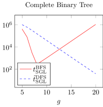
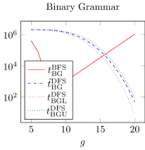
Figure 11: The expected search time of BFS and DFS graph search as a function of a single goal level $g$ with goal probability $p_{g}=0.05$ in a tree of depth $D=20$. (The part hidden by the legend is identical for both plots.) BFS has the advantage when the goal is in the higher regions of the graph, although at first the probability that no goal exists heavily influences both BFS and DFS search time. The greater connectivity of the graph in the binary grammar problem permits DFS to spend more time in the lower regions before backtracking, compared to the complete binary tree analysed in the previous section. This penalises DFS runtime when the goal is not in the very lowest regions of the tree.

It is a natural exercise to plot the expected runtime as a function of the involved parameters. Figure 11 plots the expected runtimes for a single goal level in both a binary tree and a binary grammar. BFS is better for goals close to the root and DFS graph search better when the goals are farther from the root in both models, as expected. The initially high value of BFS depends on the high likelihood of there being no goal at all when the goal level is close to the root and only contain a few nodes. When there are no goals, both BFS and DFS will search the entire space.

More surprising is the fact that the crossover occurs later in the more connected graph of the Binary Grammar. The reason is that DFS can spend longer time in the very lowest regions of the graph before backtracking due to the higher connectivity (compare Figures 1 and 6).

Decision Boundaries

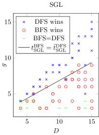
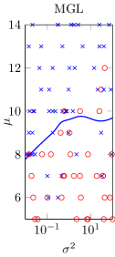
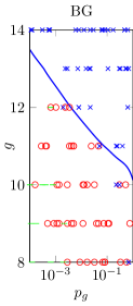
Figure 12: The left graph shows the decision boundary of Proposition 7 for the single goal level tree, The scattered points come from 100 empirical outcomes of BFS and DFS graph search times according to the varied parameters $g\in\{3,\dots,D\}$ and $D\in\{4,\dots,15\}$. The decision boundary gets $79\%$ of the winners correct. The middle graph shows the decision boundary for the Gaussian tree given by Propositions 9 and 10. The scattered points are based on 100 independently generated trees with depth $D=14$ and uniformly sampled parameters $\mu\in\{5,\dots,14\}$ and $\log(\sigma^{2})\in[-2,2]$. The most deciding feature is the goal peak $\mu$, but DFS also benefits from a smaller $\sigma^{2}$. The decision boundary gets $74\%$ of the winners correct. The right graph shows the decision boundary predicted by Corollaries 30 and 31 for the binary grammar. The scattered points are based on 100 independently generated binary grammar problems of depth $D=14$ with uniformly sampled (single) goal level $g\in\{8,\dots,14\}$ and $\log(p_{g})\in[-4,0]$. DFS benefits from a deeper goal level and higher goal probability compared to BFS. The decision boundary gets $87\%$ of the instances correct. Most ties (green dashes) are due to no goal being present.

By comparing the expected runtimes of Propositions 6 and 5; of Propositions 9 and 10; and of Corollaries 30 and 31, decision boundaries of which algorithm is the better can be obtained. Figure 12 shows these boundaries together with actual outcomes of which algorithm was faster on randomly generated instances with the given parameters.

The single goal level plot shows that BFS likes goals closer to the root, and that decision boundary given by Proposition 7 predicts the winner almost perfectly. It only fails in instances very close to the boundary.

In the decision boundary for the tree with multiple goal levels, we plot the decision boundary as a function of goal peak and goal spread in the Gaussian binary tree model. In addition to finding that BFS prefers a higher goal peak (lower $\mu$), we find that BFS also benefits relative to DFS from a greater spread $\sigma$. We can explain this result in light of Proposition 7. Roughly, a level is relevant only if it has high enough goal probability that there is a substantial chance the level has a goal. For the relevant levels, a high goal probability $(\geq 0.2)$, will make the level give the same expected search time to both BFS and DFS if it is located midway between 0 and $D$. For smaller goal probabilities, e.g. $p_{i}\approx 2^{-2k}$, level $i$ will benefit BFS more than DFS if $i<D/2-k$. Now, when the spread is low, only a single level is relevant (the mean level $\mu$) and it has high goal probability (as much as $p_{\mu}=1/2$). When the spread increases, BFS is benefited in two ways: First, the probability $p_{\mu}$ decreases, which benefits BFS according to Proposition 7. Second, additional levels $\mu-1$ and $\mu+1$ become relevant. As their goal probabilities are small, BFS will benefit from both of those levels unless $\mu$ is significantly closer to $D$ than to 0. The prediction accuracy is slightly lower than in the single goal level case, plausibly due to the increased random component of the goal model.

Finally, with the binary grammar, we experiment with adjusting the goal probability and the goal level. It can be seen that DFS clearly benefits from a higher goal probability to a much larger extent than BFS. Increasing the goal probability by a factor 10 shifts the advantage about as much as shifting the goal level by 1. It is unsurprising that DFS benefits from a high goal probability, since when the goal probability is high, a random trajectory down through the graph is likely to hit a goal fast.

Overall, the decision boundaries largely match empirical outcomes.

9.2 Empirical Averages

The data reported in Tables 1, 2 and 3 is based on an average over 1000 independently generated search problems with depth $D=14$.

• The first number in each box is the empirical average,

• the second number is the analytical estimate from previous sections, and

• the third number is the percentage error of the analytical estimate.

For certain parameter settings, there is only a small chance ($<10^{-3}$) that there are no goals. In such circumstances, all 1000 generated search graphs typically inhabit a goal, and so the empirical search times will be comparatively small. However, since a tree of depth 14 has about $2^{15}\approx 3\cdot 10^{5}$ nodes (and a search algorithm must search through all of them in case there is no goal), the rarely occurring event of no goal can still influence the expected search time substantially. To avoid this sampling problem, we have ubiquitously discarded all instances where no goal is present, and compared the resulting averages to the analytical expectations conditioned on at least one goal being present. These modified analytical expectations are obtained by removing the term corresponding to ‘no goal’ and renormalising the probabilities. Details are discussed in connections to the results above. Since the calculation of the probability that no goal exists and the search time when no goal exists are both uncontroversial, there is limited reason to verify these parts experimentally.

Complete Tree

$g\backslash p_{g}$	0.001	0.01	0.1
$5$		$46$	$40$
		$47$	$40$
		$0.7\text{\,}\mathrm{\char 37\relax}$	$0.4\text{\,}\mathrm{\char 37\relax}$
$8$	$369$	$332$	$264$
	$378$	$333$	$265$
	$2.3\text{\,}\mathrm{\char 37\relax}$	$0.3\text{\,}\mathrm{\char 37\relax}$	$0.2\text{\,}\mathrm{\char 37\relax}$
$11$	$2747$	$2143$	$2056$
	$2744$	$2147$	$2057$
	$0.1\text{\,}\mathrm{\char 37\relax}$	$0.2\text{\,}\mathrm{\char 37\relax}$	$0.0\text{\,}\mathrm{\char 37\relax}$
$14$	$17\,364.820$	$16\,482.680$	$16\,392.680$
	$17\,383.000$	$16\,483.000$	$16\,393.000$
	$0.1\text{\,}\mathrm{\char 37\relax}$	$0.0\text{\,}\mathrm{\char 37\relax}$	$0.0\text{\,}\mathrm{\char 37\relax}$

(a) BFS single goal level

$g\backslash p_{g}$	0.001	0.01	0.1
$5$		$14\,678$	$8205$
		$14\,998$	$8052$
		$2.199\,999\,999\,999\,999\,7\text{\,}\mathrm{\char 37\relax}$	$1.9\text{\,}\mathrm{\char 37\relax}$
$8$	$14\,533$	$9832$	$1104$
	$15\,623.370$	$9966.700$	$1154.000$
	$7.5\text{\,}\mathrm{\char 37\relax}$	$1.4\text{\,}\mathrm{\char 37\relax}$	$4.5\text{\,}\mathrm{\char 37\relax}$
$11$	$11\,200$	$1534$	$152$
	$11\,138$	$1586$	$146$
	$0.5\text{\,}\mathrm{\char 37\relax}$	$3.400\,000\,000\,000\,000\,4\text{\,}\mathrm{\char 37\relax}$	$4.100\,000\,000\,000\,000\,5\text{\,}\mathrm{\char 37\relax}$
$14$	$1971$	$208$	$30$
	$2000$	$200$	$20$
	$1.400\,000\,000\,000\,000\,1\text{\,}\mathrm{\char 37\relax}$	$4.2\text{\,}\mathrm{\char 37\relax}$	$34.599\,999\,999\,999\,994\text{\,}\mathrm{\char 37\relax}$

(b) DFS single goal level

Table 1: BFS and DFS performance in the single goal level model with depth $D=14$, where $g$ is the goal level and $p_{g}$ the goal probability. Each box contains empirical average/analytical expectation/error percentage.

The accuracy of the predictions of Propositions 5 and 6 are shown in Table 1, and the accuracy of Propositions 9 and 10 in Table 2. The relative error is always small for BFS ($<10\%$). For DFS the error is generally within $20\%$, except when the search time is small ($<35$ nodes are explored), in which case the absolute error is always small. These boundary plots show that the analysis generally predicts the correct BFS vs. DFS winner.

As discussed in Section 4, our BFS results can be compared with the worst case IDA* result $2^{g+2}$ by Korf et al., (2001). Comparing Korf et al.,’s results to a doubling of the empirical averages in Table 1(a) still yields that Korf et al.,’s predictions are 33-50% overestimates compared to empirical outcomes. This is unsurprising given that Korf et al.,’s estimates are intended for the worst case. We did not find a natural way of adapting Korf et al.,’s results to the multiple goal level scenarios.

$\mu\backslash\sigma$​​​​​​	0.1	1	10	100
5	$37$	$43$	$90$	$225$
	$37$	$41$	$83$	$210$
	$0.537\,056\,928\,034\text{\,}\mathrm{\char 37\relax}$	$5.028\,571\,428\,57\text{\,}\mathrm{\char 37\relax}$	$7.868\,383\,404\,86\text{\,}\mathrm{\char 37\relax}$	$6.365\,776\,731\,38\text{\,}\mathrm{\char 37\relax}$
8	$261$	$171$	$119$	$211$
	$261$	$173$	$119$	$210$
	$0.0\text{\,}\mathrm{\char 37\relax}$	$0.895\,973\,935\,304\text{\,}\mathrm{\char 37\relax}$	$0.167\,238\,063\,383\text{\,}\mathrm{\char 37\relax}$	$0.457\,655\,107\,337\text{\,}\mathrm{\char 37\relax}$
11	$2048$	$952$	$303$	$249$
	$2049$	$952$	$304$	$247$
	$0.0\text{\,}\mathrm{\char 37\relax}$	$0.0\text{\,}\mathrm{\char 37\relax}$	$0.345\,497\,022\,145\text{\,}\mathrm{\char 37\relax}$	$0.781\,688\,447\,046\text{\,}\mathrm{\char 37\relax}$
14​	$16\,210$	$5159$	$968$	$332$
	​​$16\,152$	$5136$	$960$	$329$
	$0.355\,450\,821\,695\text{\,}\mathrm{\char 37\relax}$	$0.448\,882\,445\,518\text{\,}\mathrm{\char 37\relax}$	$0.816\,710\,031\,801\text{\,}\mathrm{\char 37\relax}$	$0.940\,335\,276\,092\text{\,}\mathrm{\char 37\relax}$

(a) BFS multi goal level

$\mu\backslash\sigma$​​​​	0.1	1	10	100
5	$5374$	$8572$	$3404$	$385$
	$5949$	$10\,073$	$3476$	$379$
	$10.693\,612\,040\,9\text{\,}\mathrm{\char 37\relax}$	$17.515\,999\,356\,1\text{\,}\mathrm{\char 37\relax}$	$2.117\,298\,762\,63\text{\,}\mathrm{\char 37\relax}$	$1.736\,516\,082\,21\text{\,}\mathrm{\char 37\relax}$
8	$677$	$1233$	$454$	$252$
	$743$	$1259$	$473$	$259$
	$9.788\,433\,998\,2\text{\,}\mathrm{\char 37\relax}$	$2.075\,193\,333\,44\text{\,}\mathrm{\char 37\relax}$	$4.184\,082\,009\,77\text{\,}\mathrm{\char 37\relax}$	$2.897\,403\,419\,89\text{\,}\mathrm{\char 37\relax}$
11	$97.38$	$168$	$117$	$210$
	$92$	$157$	$106$	$211$
	$4.549\,188\,745\,12\text{\,}\mathrm{\char 37\relax}$	$6.354\,117\,087\,1\text{\,}\mathrm{\char 37\relax}$	$9.103\,295\,580\,35\text{\,}\mathrm{\char 37\relax}$	$0.799\,961\,906\,576\text{\,}\mathrm{\char 37\relax}$
14	$24$	$43$	$81$	$213$
	$11$	$33$	$74$	$205$
	$51.583\,333\,333\,3\text{\,}\mathrm{\char 37\relax}$	$24.181\,650\,530\,2\text{\,}\mathrm{\char 37\relax}$	$8.917\,431\,192\,66\text{\,}\mathrm{\char 37\relax}$	$4.025\,840\,277\,13\text{\,}\mathrm{\char 37\relax}$

(b) DFS multi goal level

Table 2: BFS and DFS performance in Gaussian binary trees with depth $D=14$. Each box contains empirical average/analytical expectation/error percentage.

Grammar

The binary grammar model of Section 8.1 serves to verify the general estimates of Propositions 14 and 17. The results are shown in Table 3. The estimates for BFS are accurate as usual ($<3\%$ error). With few exceptions, the lower and the upper bounds $t^{\mathrm{DFS}}_{\mathrm{BGL}}$ and $t^{\mathrm{DFS}}_{\mathrm{BGU}}$ of Corollary 31 for DFS differ by at most $50\%$ on the respective sides from the true (empirical) average. The arithmetic mean $\tilde{t}^{\mathrm{DFS}}_{\mathrm{BG}}$ often give surprisingly accurate predictions ($<4\%$) except when $t^{\mathrm{DFS}}_{\mathrm{BGL}}$ and $t^{\mathrm{DFS}}_{\mathrm{BGU}}$ leave wide margins as to the expected search time (when $g=14$, the margin is up to $84\%$ downwards and $125\%$ upwards). Even then, the $\tilde{t}^{\mathrm{DFS}}_{\mathrm{BG}}$ error remains within $30\%$.

$g\backslash p_{g}$	0.001	0.01	0.1
$5$		$47$	$41$
		$47$	$40$
		$0.2\text{\,}\mathrm{\char 37\relax}$	$1.700\,000\,000\,000\,000\,2\text{\,}\mathrm{\char 37\relax}$
$8$	$376$	$332$	$266$
	$378$	$333$	$265$
	$0.6\text{\,}\mathrm{\char 37\relax}$	$0.4\text{\,}\mathrm{\char 37\relax}$	$0.3\text{\,}\mathrm{\char 37\relax}$
$11$	$2751$	$2145$	$2058$
	$2744$	$2147$	$2057$
	$0.3\text{\,}\mathrm{\char 37\relax}$	$0.1\text{\,}\mathrm{\char 37\relax}$	$0.0\text{\,}\mathrm{\char 37\relax}$
$14$	$17\,372$	$16\,479$	$16\,394$
	$17\,383$	$16\,483$	$16\,393$
	$0.1\text{\,}\mathrm{\char 37\relax}$	$0.0\text{\,}\mathrm{\char 37\relax}$	$0.0\text{\,}\mathrm{\char 37\relax}$

(a) BFS $t^{\mathrm{BFS}}_{\mathrm{BG}}$

$g\backslash p_{g}$	0.001	0.01	0.1
$5$		$30\,915$	$27\,837$
		$31\,365$	$30\,186$
		$1.5\text{\,}\mathrm{\char 37\relax}$	$8.4\text{\,}\mathrm{\char 37\relax}$
$8$	$27\,999$	$25\,157$	$15\,494$
	$27\,407$	$24\,421$	$15\,203$
	$2.1\text{\,}\mathrm{\char 37\relax}$	$2.900\,000\,000\,000\,000\,4\text{\,}\mathrm{\char 37\relax}$	$1.9\text{\,}\mathrm{\char 37\relax}$
$11$	$17\,284$	$5932$	$1815$
	$16\,787$	$5806$	$1788$
	$2.900\,000\,000\,000\,000\,4\text{\,}\mathrm{\char 37\relax}$	$2.1\text{\,}\mathrm{\char 37\relax}$	$1.5\text{\,}\mathrm{\char 37\relax}$
$14$	$1304$	$122$	$26$
	$1522$	$165$	$20$
	$16.7\text{\,}\mathrm{\char 37\relax}$	$34.8\text{\,}\mathrm{\char 37\relax}$	$21.6\text{\,}\mathrm{\char 37\relax}$

(b) Average DFS $\tilde{t}^{\mathrm{DFS}}_{\mathrm{BG}}$

$g\backslash p_{g}$	0.001	0.01	0.1
$5$		$30\,915$	$27\,837$
		$30\,711$	$29\,080$
		$0.700\,000\,000\,000\,000\,1\text{\,}\mathrm{\char 37\relax}$	$4.5\text{\,}\mathrm{\char 37\relax}$
$8$	$27\,999$	$25\,157$	$15\,494$
	$25\,737$	$22\,151$	$12\,072$
	$8.1\text{\,}\mathrm{\char 37\relax}$	$11.899\,999\,999\,999\,999\text{\,}\mathrm{\char 37\relax}$	$22.1\text{\,}\mathrm{\char 37\relax}$
$11$	$17\,284$	$5932$	$1815$
	$14\,164$	$3822$	$919$
	$18.099\,999\,999\,999\,998\text{\,}\mathrm{\char 37\relax}$	$35.6\text{\,}\mathrm{\char 37\relax}$	$49.4\text{\,}\mathrm{\char 37\relax}$
$14$	$1304$	$122$	$26$
	$809$	$54$	$4$
	$38.0\text{\,}\mathrm{\char 37\relax}$	$55.7\text{\,}\mathrm{\char 37\relax}$	$84.399\,999\,999\,999\,99\text{\,}\mathrm{\char 37\relax}$

(c) Lower DFS $t^{\mathrm{DFS}}_{\mathrm{BGL}}$

$g\backslash p_{g}$	0.001	0.01	0.1
$5$		$30\,915$	$27\,837$
		$32\,019$	$31\,293$
		$3.599\,999\,999\,999\,999\,6\text{\,}\mathrm{\char 37\relax}$	$12.4\text{\,}\mathrm{\char 37\relax}$
$8$	$27\,999$	$25\,157$	$15\,494$
	$29\,075$	$26\,690$	$18\,335$
	$3.8\text{\,}\mathrm{\char 37\relax}$	$6.1\text{\,}\mathrm{\char 37\relax}$	$18.3\text{\,}\mathrm{\char 37\relax}$
$11$	$17\,283$	$5932$	$1815$
	$19\,411$	$7789$	$2657$
	$12.3\text{\,}\mathrm{\char 37\relax}$	$31.3\text{\,}\mathrm{\char 37\relax}$	$46.400\,000\,000\,000\,006\text{\,}\mathrm{\char 37\relax}$
$14$	$1304$	$122$	$25$
	$2236$	$275$	$36$
	$71.5\text{\,}\mathrm{\char 37\relax}$	$125.299\,999\,999\,999\,98\text{\,}\mathrm{\char 37\relax}$	$41.099\,999\,999\,999\,994\text{\,}\mathrm{\char 37\relax}$

(d) Upper DFS $t^{\mathrm{DFS}}_{\mathrm{BGU}}$

Table 3: BFS and DFS performance in binary grammars of depth $D=14$. Empirical DFS performance is compared to the upper and lower bounds of Corollary 31, as well as their arithmetic average. In these experiments, goals are distributed on a single goal level $g$ with goal probability $p_{g}$. The BFS estimates $t^{\mathrm{BFS}}_{\mathrm{BG}}$ are highly accurate, and the averaged DFS estimates $\tilde{t}^{\mathrm{DFS}}_{\mathrm{BG}}$ are mostly accurate. Each box contains empirical average/analytical expectation/error percentage.

9.3 N-Puzzle

(e,2em,2em)—c:c:c——c:c:c— 6 & 8
3 4 7
2 5 1

Figure 13: 8-Puzzle. At any stage, the empty tile may be swapped with an adjacent tile. The goal is to sort the tiles with the empty tile at the bottom right.

In this section, we apply the theory of Sections 6 and 7 to the 8-Puzzle problem (Figure 13), estimating expected search time from a local sample. We focus on evaluating BFS (graph search) and DFS tree search for this problem, as DFS graph search consistently cut itself off from significant portions of the 8-puzzle search space (see discussion in Section 3.2, including Figure 2 on Figure 2).

Local branching factors

The 8-Puzzle appears to approximately satisfy uniformity 21, as can be seen in Figure 14.

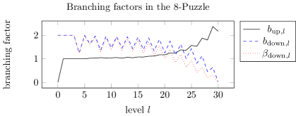
Figure 14: Average branching factors as a function of depth. Here $b_{\mathrm{up},l}$ is short for average the average value of $b_{\mathrm{up}}(v)$ given that $\mathrm{level}(v)=l$, and similarly for $b_{\mathrm{down},l}$. The branching factors roughly satisfy the uniformity assumption up until level 22. The majority of the nodes of the 8-puzzle are on level 22 or above. Note also that the global branching factor $\beta_{\mathrm{down}}$ is slightly lower than the local branching factor $b_{\mathrm{down}}$, as expected.

Running BFS up until depth 9 and using the average from levels 6 to 9, we find that

• $b_{\mathrm{up}}\approx 1.035$

• $b_{\mathrm{side}}=0$ (due to invariants in the N-Puzzle, different nodes can only be reached in even and odd number of steps)

• $b_{\mathrm{down}}\approx 1.80$

• $\beta_{\mathrm{up}}\approx b_{\mathrm{up}}$ (the data was insufficient to get a better estimate)

• $\beta_{\mathrm{down}}\approx 1.66$

Despite using levels a few steps away from the start, the parameters vary somewhat depending on whether the empty tile started in a corner, in the middle of an edge, or in the middle. We use a weighted average according to the distribution of a randomly sampled problem, with the middle edge and corner cases having relative weight 4 each, and the middle case having relative weight 1.

The branching factors are core to our theory. They allow us to approximate the length-to-depth distribution $P_{n}(d)$ for the probability at being at depth $d$ after $n$ steps. The correspondence between our approximation (9) of $P_{n}(d)$ on page 9 and the empirical distribution of search depths is shown in Figure 15.

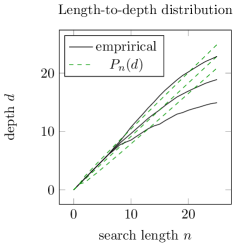
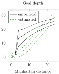
Figure 15: Left, the length-to-depth distribution $P_{n}(d)$ matched to the empirical depth-distribution. Right, the estimated goal distribution compared to the empirical goal distribution. All distributions are shown together with one standard deviation above and below. $P_{n}(d$ approximately matches the empirical distribution until about level 20, where the branching factor estimates ceases to be valid. The goal distribution only roughly matches the truth.

Goal probability estimates

A natural problem feature of N-Puzzle instances is the Manhattan distance $\mathrm{mh}(v_{0},v^{*})$ between the starting node $v_{0}$ and the goal node $v^{*}$ (Russell and Norvig,, 2010). An N-puzzle configuration can be represented with the coordinates for the different tiles, $v=\langle(x_{0},y_{0}),(x_{1},y_{1}),\dots,(x_{n},y_{n})\rangle$ where $(x_{i},y_{i})$ is the coordinates of tile $i$ and $i=0$ represents the empty tile. The Manhattan distance is then

$$\mathrm{mh}(v,u)=\sum_{i=0}^{N}|x_{i}^{u}-x_{i}^{v}|+|y_{i}^{u}-y_{i}^{v}|.$$

Note that $\mathrm{mh}(v_{0},v^{*})$ needs to be divided by 2 in order to be an admissible heuristic.

Investigating the correlation between the Manhattan distance $\mathrm{mh}$ and the actual distance $\mathrm{dist}$, we find that $\mathbb{E}[\mathrm{dist}(v,u)\mid\mathrm{mh}(v,u)=m]\approx 1.5m$ and $\mathrm{Std}(\mathrm{dist}(v,u)\mid\mathrm{mh}(v,u)=m)\approx 3.5$. This gives us a mean goal level $\mu=1.5\mathrm{mh}(v_{0},v^{*})$ and standard deviation $\sigma=3.5$. We use a Gaussian-inspired goal probability vector ${\mathbf{p}}^{\text{n-puzzle}}$ with $p^{\text{n-puzzle}}_{i}=c\cdot e^{-\frac{(i-\mu)^{2}}{2\cdot\sigma^{2}}}/\beta_{\mathrm{down}}^{i}$ where $c=1/\sum_{i=-\infty}^{\infty}e^{-\frac{(i-\mu)^{2}}{2\cdot\sigma^{2}}}$ is a normalising constant and $\beta_{\mathrm{down}}^{i}$ is the expected number of nodes on level $i$ based on the global branching factor $\beta_{\mathrm{down}}$.

The theoretical goal distribution is matched against the true goal distribution in Figure 15.

Search time estimates

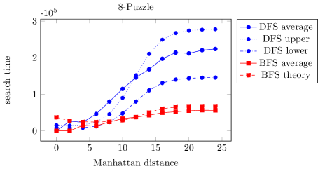
Figure 16: 8-Puzzle search times for DFS tree search and BFS. The empirical averages are displayed together with the theoretical bounds for DFS, and the theoretical estimate for BFS. As expected, DFS tree search expands more nodes than BFS. Overall, there is a strong match between theory and practice, with average DFS search times generally being contained within the bounds, and BFS search times closely following their theoretical estimate. The empirical averages are based on a 100 runs per Manhattan distance.

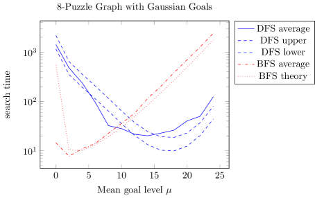
Figure 17: Search times for DFS tree search and BFS in an 8-Puzzle graph with nodes distributed according to the Gaussian goal probability vector $p_{i}=\min\left\{1,c\cdot e^{(i-\mu)^{2}/(2\sigma^{2})}\right\}$ where $c=\sum_{i=-\infty}^{\infty}e^{(i-\mu)^{2}/(2\sigma^{2})}$ is a normalising constant. BFS is better than DFS for mean goal$\mu$ between 1 and 9, and DFS is better for $\mu$ between 10 and 20. The theoretical bounds slightly overestimate the search time of DFS for lower $\mu$, and slightly underestimates DFS search time for higher $\mu$, possibly as a result of the branching factors estimates being based on the middle levels of the graph. The empirical averages are based on a 100 runs per mean goal level.

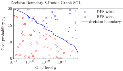
Figure 18: Empirical outcomes together with the theoretical decision boundary between DFS tree search and BFS in a modified 8-puzzle graph with a single goal level $g$ with goal probability $p_{g}$. As expected, DFS benefits by lower levels with higher goal probability. The decision boundary classifies $90\%$ of the points correctly.

We compare the search time estimates based on the above parameters and the theory developed in Sections 6 and 7 with empirical averages. The results are displayed in Figure 16. Our averages are based on 100 randomly sampled problems of each occurring Manhattan distance. To avoid the changing dynamics of the lowest levels (see Figure 14), we set the radius of search to 20.

As can be seen in Figure 16, our theoretical model predicts expected search time reasonably accurately. We find it encouraging that our methods allow us to predict the search time of especially DFS so well. The theoretical estimates are off slightly for the levels where the goal distribution is inaccurate (Figure 15). To separate the sources of error, we also investigate two 8-Puzzle search problems with artificially sampled goals. In these problems, we also take the opportunity to increase the number of goals to give DFS a better chance in comparison. In the first problem, we used a Gaussian goal probability vector (Figure 17). In the second problem, we used single goal level with varying goal probability (Figure 18).

As expected, DFS beats BFS when many goals are located far from the start, which is the case in the Gaussian model in Figure 17 with high $\mu$. In the single goal level model high $g$ means goals located far from the root, and high $p_{g}$ means high chance of random walking into one. The points of DFS takeover are well predicted by our theory (Figures 17 and 18). In the original 8-puzzle, DFS struggles to random walk into the single goal, and always needs to explore a substantial portion of the graph in order to find a goal (note that Figure 16 is not a logplot, as opposed to Figure 17). Unsurprisingly, BFS graph search is virtually always faster than DFS tree search in this setting.

10 Adapting Results to Heuristic Search

In many situations, heuristic search methods like A* or heuristic DFS are better options than the uninformed methods of BFS and DFS discussed in this paper. In this section, we discuss how our results in previous sections can be generalised to heuristic search.

Definition 36 (Heuristic levels).

Let $g:S\to\mathbb{R}$ be a consistent heuristic function, and let $f(v)\geq\mathrm{dist}(v_{0},v)$ be the length of the current search path reaching $v$. Let $h(v)=f(v)+g(v)$. We define two generalisations of Definition 11: Let the $g$-level $l$ be the set of nodes with $g(v)=l$, and let the $h$-level $l$ be the set of nodes with $h(v)=l$.

A popular method for heuristic search is A*, which can be seen as a generalisation of BFS. The main difference between BFS and A* is that while BFS expands the search graph according to levels, A* expands the graph according to $h$-levels. In analysing iterative deepening A* in trees, Korf et al., (2001) has argued that the downwards branching factors remain the same when considering the considering the tree layered by $g$-levels instead of levels, and that the goal probability vector is shifted by a constant $k$ depending on the heuristic (so $p_{g}$ for BFS is $p_{g-k}$ for A*). Other researchers prefer to model the effect of the heuristic as reducing the branching factor (Russell and Norvig,, 2010, p. 111). It is an empirical question which model works best in our case. Investigating this constitutes a promising line of future work.

path $\leftarrow$ empty list

DFS-tree-rec($N$, $C$, start node, path, radius, $g$)

function Heuristic-DFS-rec($N$, $C$, $u$, path, radius, $g$)

     path.append($u$)

     if $C(u)$ then return $u$      

     if length(path) $<$ radius then

         ranked-neighbours $\leftarrow$ sort($N(u)\setminus$path, $g$)$\triangleright$ with low $g$ first

         for $v$ in ranked-neighbours do

              DFS-tree-rec($N$, $C$, $v$, path, radius, $g$)               

Algorithm 4 Heuristic DFS tree search

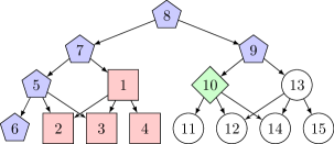
Figure 19: Heuristic DFS may be seen as a DFS search that follows $g$-levels instead of levels, and that possibly “backtracks” up above the initial $g$-level that it started at.

Heuristically guided versions of DFS include Beam search and heuristic DFS (see Algorithm 4). While A* follows $h$-levels, it is most natural to understand heuristic DFS to follow $g$-levels (see Figure 19). Heuristic DFS starts at some intermediate $g$-level. Once it exhausts nodes on $g$-levels below it (assuming it does not find a goal there), it may find its way to higher $g$-levels than it started at. This may be seen as a generalised notion of backtracking. Extending our theory of DFS search time to heuristic DFS would involve finding a theory for $g$-level branching factors, and making the generalised notion of backtracking precise.

11 Summary and Outlook

Search and optimisation problems appear in different flavors throughout the field of artificial intelligence; in planning, problem solving, games, and learning. Therefore even minor improvements to search performance can potentially lead to gains in many aspects of intelligent systems. It is even possible to equate intelligence with (Bayesian expectimax) optimisation performance (Legg and Hutter,, 2007).

Summary

In this paper we have derived analytical results for expected runtime of BFS and DFS. Sections 4 and 5 focused on BFS and DFS tree search where explored nodes were not remembered. A vector ${\mathbf{p}}=[p_{1},\dots,p_{D}]$ described a priori goal probabilities for the different levels of the tree. This concrete but general model of goal distribution allowed us to calculate approximate closed-form expression of both BFS and DFS average runtime. Earlier studies have only addressed worst case runtimes: For example Knuth, (1975) and followers for DFS; Korf et al., (2001) and followers for IDA*, a linear space version of BFS.

Section 6 generalised the model of Sections 4 and 5 to non-tree graphs. In addition to the goal probability vector ${\mathbf{p}}$, the graph search analysis required additional structural information in the form of a length-to-depth counter $L$, which was inferred from branching factors in Section 7. The DFS graph search estimates also took the form of less precise bounds. The analysis of Section 6 does not supersede the analysis in Sections 4 and 5, as the bounds of Section 6 become uninformative when the graph is a tree. The analytical results are generally consistent with empirical outcomes.

In Section 10 we also outlined how our results can be extended to heuristic search.

The value of expected search time

Several applications are naturally directed to maximising expected utility, including games and reinforcement learning. In such contexts, average performance is often more important than worst case performance. Indeed, in our model, worst case performance is always $2^{D+1}$ for both BFS and DFS since it is not a priori necessary that a goal exists. Our expected runtime estimates are much more informative.

Being able to estimate expected search time for BFS and DFS is valuable for several reasons. First, and most obvious, it can be used for allocating resources, and in deciding whether a problem is approachable with BFS or DFS at all. Second, expected search time can guide the choice of algorithm, and the choice of graph representation. Choosing the best algorithm and the best representation can improve performance substantially. Third, the results also offer theoretical insight into BFS and DFS. As BFS and DFS are opposites, and in a sense are the most fundamental ways to search, we have high hopes that our results and techniques can be useful both in the construction of new search algorithms, and in the analysis of existing ones. For example, A* and IDA* may be viewed as generalisations of BFS, and Beam Search and Greedy Best-First as generalisations of DFS. We find the DFS tree search results for graphs developed in Sections 6 and 7 especially promising, and believe they may find use outside the domain considered in this paper.

A List of notation

$P$	Probability
$X$, $Y$	Random variables
$\mathbb{E}[\,\cdot\,]$	Expectation of a random variable
$\mathrm{tc}(p,m)$	Expectation of a truncated geometric variable with parameters $p$ and $m$
$O$	Big-O notation
$\mathit{EC}$	Edge cost
$h$	Heuristic function
$g$	Accumulated path cost from start node
$Q$	Objective function
$D$	Maximum search depth/level
$D^{\prime}$	Radius of search (maximum path length DFS search)
$p_{g}$	Goal probability at a single goal level $g$
$p_{k}$	Goal probability for a level $k$
$q_{k}$	$1-p_{k}$
${\mathbf{p}}$	Vector of probabilities for multiple goal levels
$\mu,\sigma^{2}$	Goal peak and goal spread in Gaussian binary tree
$\Gamma$	Probability that a goal exists
$\Gamma_{k}$	Probability that level $k$ has a goal
$F_{k}$	Probability that level $k$ has the first goal
$t^{\mathrm{BFS}}_{\mathrm{SGL}}$, $\tilde{t}^{\mathrm{DFS}}_{\mathrm{SGL}}$	Expected BFS search time and approximate expected DFS search time in a complete tree with a single goal level
$t^{\mathrm{BFS}}_{\mathrm{MGL}}$, $\tilde{t}^{\mathrm{DFS}}_{\mathrm{MGL}}$	Expected BFS search time and approximate expected DFS search time in a complete tree with multiple goal levels
$t^{\mathrm{BFS}}_{\mathrm{CB}}$, $\tilde{t}^{\mathrm{DFS}}_{\mathrm{CB}}$	Expected BFS search time and approximate expected DFS search time in a graph with colliding branches
$t^{\mathrm{BFS}}_{\mathrm{BG}}$, $\tilde{t}^{\mathrm{DFS}}_{\mathrm{BG}}$	Expected BFS search time and approximate expected DFS search time in the binary grammar problem
$t^{\mathrm{BFS}}_{\mathrm{FG}}$, $\tilde{t}^{\mathrm{DFS}}_{\mathrm{FG}}$	Expected BFS search time and approximate expected DFS search time in the full grammar problem
$\mathrm{dist}$	Distance (shortest path between two nodes)
$\mathrm{level}$	Level (distance from start node)
$\delta_{n}$	The first node on level $n$ reached by DFS
$K(l,d,r)$, $\overline{K}(l,d,r)$	Depth-to-depth counters, counting the number of (unique and non-unique) level $d$ descendants are reachable from level $l$ in at most $r$ steps
$L(n,d)$, $\overline{L}(n,d)$	Length-to-depth counters, counting the number of (unique and non-unique) level $d$ descendants are reachable after an average $n$ step path (i.e. from $\delta_{n}$)
$L^{\mathrm{FG}}$, $L^{\mathrm{BG}}$	Length-to-depth counts for the binary grammar problem and the full grammar problem
$l,d$	Level/depth in graph
$n$	Path length for search in graph
$A_{n,d}$	Number of nodes reachable from $\delta_{n}$ not reachable from $\delta_{n+1}$
$S_{n}$	Descendants of $\delta_{n}$
$T_{n}$	Descendants of $\delta_{n}$ that are not descendants of $\delta_{n+1}$
$U_{n}$	The number of nodes above level $n$.
$\tau_{n}$	The probability that $T_{n}$ contains a goal (Lemma 13)
$\phi_{n}$	The probability that $T_{n}$ inhabits the first goal
$b$	Branching factor trees
$b_{\mathrm{dir}}$, $\beta_{\mathrm{dir}}$	Local and global branching factors in graphs for $\mathrm{dir}\in\{\mathrm{up},\mathrm{side},\mathrm{down}\}$
$p_{\mathrm{dir}}$	Average probability of moving on level in direction $\mathrm{dir}$
$p_{\mathrm{dir}_{1},\mathrm{dir}_{2}}$	Probability of moving one level in direction $\mathrm{dir}_{2}$ given came from direction $\mathrm{dir}_{2}$
${\mathbf{p}}^{\text{n-puzzle}}$	Goal probability vector for the 8-puzzle
$P_{n}(d)$	Probability at being at depth $d$ after travelling $n$ steps
$\epsilon$	Empty string

References

- Aarts and Lenstra, (2003) Aarts, E. and Lenstra, J. K., editors (2003). Local search in combinatorial optimization.
- Arbelaez Rodriguez, (2011) Arbelaez Rodriguez, A. (2011). Learning During Search. Phd thesis, University of Paris-Sud.
- Burke et al., (2003) Burke, E., Hart, E., Kendall, G., Newall, J., Ross, P., and Schulenburg, S. (2003). Hyper Heuristics: an emerging direction in modern search technology. In Glover, F. and Kochenberger, G. A., editors, Handbook of Metaheuristics, pages 457–474. Springer.
- Burke et al., (2013) Burke, E. K., Gendreau, M., Hyde, M., Kendall, G., Ochoa 1ã, G., Zcan, E., and Qu, R. (2013). Hyper-heuristics: a survey of the state of the art. Journal of the Operational Research Society, 64:1695–1724.
- Chen, (1992) Chen, P. C. (1992). Heuristic Sampling: A Method for Predicting the Performance of Tree Searching Programs. SIAM Journal on Computing, 21(2):295–315.
- Dejong and Mooney, (1986) Dejong, G. and Mooney, R. (1986). Explanation-based Learning: An Alternative View. Machine Learning, 1(2):145–176.
- Domshlak et al., (2012) Domshlak, C., Karpas, E., and Markovitch, S. (2012). Online speedup learning for optimal planning. Journal of Artificial Intelligence Research, 44:709–755.
- Edelkamp and Korf, (1998) Edelkamp, S. and Korf, R. E. (1998). The Branching Factor of Regular Search Spaces. In AAAI, pages 299–304.
- Edelkamp and Schrödl, (2012) Edelkamp, S. and Schrödl, S. (2012). Heuristic Search. Morgan Kaufmann Publishers Inc.
- Etzioni, (1993) Etzioni, O. (1993). Acquiring search-control knowledge via static analysis. Artificial Intelligence, 62:255–301.
- (11) Everitt, T. and Hutter, M. (2015a). Analytical Results on the BFS vs. DFS Algorithm Selection Problem. Part I: Tree Search. In 28th Australasian Joint Conference on Artificial Intelligence, pages 157–165.
- (12) Everitt, T. and Hutter, M. (2015b). Analytical Results on the BFS vs. DFS Algorithm Selection Problem. Part II: Graph Search. In 28th Australasian Joint Conference on Artificial Intelligence, pages 166–178.
- Fink, (1998) Fink, E. (1998). How to Solve It Automatically: Selection Among Problem-Solving Methods. In Proceedings of the Fourth International Conference on Artificial Intelligence Planning Systems, pages 128–136.
- Haim and Walsh, (2008) Haim, S. and Walsh, T. (2008). Online estimation of SAT solving runtime. In Theory and Applications of Satisfiability Testing, volume 4996 LNCS, pages 133–138. Springer.
- Hoos, (2012) Hoos, H. H. (2012). Programming by optimization. Communications of the ACM, 55(2):70.
- Hopcroft and Ullman, (1979) Hopcroft, J. E. and Ullman, J. D. (1979). Introduction to automata theory, languages, and computation. Addison-Weasly.
- Hutter et al., (2014) Hutter, F., Xu, L., Hoos, H. H., and Leyton-Brown, K. (2014). Algorithm runtime prediction: Methods & evaluation. Artificial Intelligence, 206(1):79–111.
- Kilby et al., (2006) Kilby, P., Slaney, J., Thiébaux, S., and Walsh, T. (2006). Estimating Search Tree Size. In Proc. of the 21st National Conf. of Artificial Intelligence, AAAI, Menlo Park.
- Knuth, (1975) Knuth, D. E. (1975). Estimating the efficiency of backtrack programs. Mathematics of Computation, 29(129):122–122.
- Korf et al., (2001) Korf, R. E., Reid, M., and Edelkamp, S. (2001). Time complexity of iterative-deepening-A*. Artificial Intelligence, 129(1-2):199–218.
- Kotthoff, (2014) Kotthoff, L. (2014). Algorithm Selection for Combinatorial Search Problems: A Survey. AI Magazine, pages 1–17.
- Leckie and Zukerman, (1998) Leckie, C. and Zukerman, I. (1998). Inductive learning of search control rules for planning. Artificial Intelligence, 101:63–98.
- Legg and Hutter, (2007) Legg, S. and Hutter, M. (2007). Universal Intelligence. Minds & Machines, 17(4):391–444.
- Lelis, (2013) Lelis, L. (2013). Cluster-and-Conquer: a Paradigm for Solving State-Space Problems. Phd thesis, University of Alberta.
- Minton, (1988) Minton, S. (1988). Learning Search Control Knowledge: An Explanation-Based Approach. Kluwer Academic Publishers.
- Minton, (1990) Minton, S. (1990). Quantitative results concerning the utility of explanation-based learning. Artificial Intelligence, 42(1990):363–391.
- Mitchell et al., (1986) Mitchell, T., Keller, R., and Kedar-CabeUi, S. (1986). Explanation-based generalization: A unifying view. Machine Learning, 1(1):47–80.
- Nilsson, (1971) Nilsson, N. J. (1971). Problem-Solving Methods in Artificial Intelligence. McGraw-Hill Pub.
- Pearl, (1984) Pearl, J. (1984). Heuristics: Intelligent Search Strategies for Computer Problem Solving. Addison-Wesley.
- Peixoto, (2015) Peixoto, T. P. (2015). The graph-tool python library. figshare.
- Purdom, (1978) Purdom, P. W. (1978). Tree Size by Partial Backtracking. SIAM Journal on Computing, 7(4):481–491.
- Rice, (1975) Rice, J. R. (1975). The algorithm selection problem. Advances in Computers, 15:65–117.
- Rokicki and Kociemba, (2013) Rokicki, T. and Kociemba, H. (2013). The diameter of the rubik’s cube group is twenty. SIAM Journal on Discrete Mathematics, 27(2):1082–1105.
- Ross et al., (2002) Ross, P., Schulenburg, S., Marin-Blazquez, J. G., and Hart, E. (2002). Hyper-heuristics: learning to combine simple heuristics in bin-packing problems. In GECCO’02.
- Russell and Norvig, (2010) Russell, S. J. and Norvig, P. (2010). Artificial intelligence: a modern approach. Prentice Hall, third edition.
- Smith-Miles et al., (2014) Smith-Miles, K., Baatar, D., Wreford, B., and Lewis, R. (2014). Towards objective measures of algorithm performance across instance space. Computers & Operations Research, 45:12–24.
- Smith-Miles and Lopes, (2012) Smith-Miles, K. and Lopes, L. (2012). Measuring instance difficulty for combinatorial optimization problems. Computers and Operations Research, 39(5):875–889.
- Thayer et al., (2011) Thayer, J. T., Dionne, A. J., and Ruml, W. (2011). Learning inadmissible heuristics during search. In ICAPS.
- Thompson, (2011) Thompson, C. (2011). Metareasoning about propagators for constraint satisfaction. Phd thesis, University of Saskatchewan.
- Tolpin et al., (2013) Tolpin, D., Beja, T., Shimony, S. E., Felner, A., and Karpas, E. (2013). Towards rational deployment of multiple heuristics in a*. In Sixth Annual Symposium on Combinatorial Search.
- Tolpin et al., (2014) Tolpin, D., Betzalel, O., Felner, A., and Shimony, S. E. (2014). Rational deployment of multiple heuristics in ida. arXiv preprint arXiv:1411.6593.
- Zahavi et al., (2010) Zahavi, U., Felner, A., Burch, N., and Holte, R. C. (2010). Predicting the performance of IDA* using conditional distributions. Journal of Artificial Intelligence Research, 37:41–83.