Liquid crystal phases of two-dimensional dipolar gases and Berezinskii-Kosterlitz-Thouless melting

Abstract

Liquid crystals are phases of matter intermediate between crystals and liquids. Whereas classical liquid crystals have been known for a long time and are used in electro-optical displays, much less is known about their quantum counterparts. There is growing evidence that quantum liquid crystals play a central role in many electron systems including high temperature superconductors, but a quantitative understanding is lacking due to disorder and other complications. Here, we analyse the quantum phase diagram of a two-dimensional dipolar gas, which exhibits stripe, nematic and supersolid phases. We calculate the stiffness constants determining the stability of the nematic and stripe phases, and the melting of the stripes set by the proliferation of topological defects is analysed microscopically. Our results for the critical temperatures of these phases demonstrate that a controlled study of the interplay between quantum liquid and superfluid phases is within experimental reach for the first time, using dipolar gases.

The investigation of cold atomic gases has enabled one to study many-body physics with unrivalled experimental control and in regimes never realised before. Recent progress in trapping and cooling of gases consisting of dipolar atoms/molecules opens up a promising new research direction. The dipole-dipole interaction is long range and anisotropic, which is predicted to give rise to a number of exotic forms of matter Baranov (2008); Lahaye et al. (2009). Degenerate Fermi gases consisting of atoms with a large magnetic dipole moment have already been created Lu et al. (2012); Aikawa et al. (2014), and progress towards producing degenerate gases of fermionic molecules with an electric dipole moment is being reported Heo et al. (2012); Park et al. (2015).

Here, we analyse the quantum phases of a two-dimensional (2D) dipolar Fermi gas at non-zero temperatures $T$. This includes a stripe phase, whose low energy degrees of freedom are described by an anisotropic XY model. We determine the stiffness constants of this effective model microscopically. The finite temperature melting of the stripe phase is driven by the proliferation of topological defects called dislocations, and the corresponding Berezinskii-Kosterlitz-Thouless (BKT) critical temperature is determined by the well-known renormalisation group equations. For large tilting angles of the dipoles, the system can have additional superfluid pairing which coexists with the stripe order. We calculate the critical temperature of the superfluid transition. When the dipoles are perpendicular to the 2D plane, the critical temperature of the stripe phase is shown to vanish, and the system exhibits a nematic phase characterised by long range orientational order but no translational order. Our results demonstrate that with dipolar gases, it is within experimental reach to study quantum liquid and superfluid phases characterised by varying degrees of spontaneous translational, rotational, and gauge symmetry breaking. The interplay between such phases is believed to play an important role in many electronic materials discovered in recent decades Fradkin and Kivelson (2010); Kivelson et al. (1998); Chuang et al. (2010); Emery et al. (1999); Kohsaka et al. (2007). Moreover, our results show that one can confirm the microscopic mechanism behind the BKT transition, namely the proliferation of topological defects, simply by observing the proliferation of disclocation defects in the stripe pattern. Such an experimental verification of BKT physics has been achieved only recently using atomic gases Hadzibabic et al. (2006), whereas other experiments reported only indirect evidence of BKT physics in the bulk properties Bishop and Reppy (1978); Fiory et al. (1983); Reyren et al. (2007); Ye et al. (2010); Matthey et al. (2007); Rout and Budhani (2010); Resnick et al. (1981); Safonov et al. (1998).

I Results

We consider fermionic dipoles of mass $m$ and average areal density $n_{0}$, which are restricted to move in the $xy$ plane by a tight harmonic trapping potential $m\omega_{z}^{2}z^{2}/2$ along the $z$-direction. In the limit $\omega_{z}\gg\epsilon_{F}$, where $\epsilon_{F}=k_{F}^{2}/2m=2\pi n_{0}/m$ is the Fermi energy of a 2D non-interacting gas with areal density $n_{0}$, the system is effectively 2D with the dipoles frozen in the harmonic oscillator ground state in the $z$ direction. An external field aligns the dipoles so that their dipole moment $\bf d$ is perpendicular to the $y$-axis and forms an angle $\Theta$ with the $z$-axis. The dipole-dipole interaction is $V_{\rm d}({\bf r},z)=D^{2}(1-3\cos^{2}\theta_{rd})/(r^{2}+z^{2})^{3/2}$, where $\theta_{rd}$ is the angle between the relative displacement vector of the two dipoles $({\bf r},z)$ with ${\bf r}=(x,y)$ and the dipole moment $\bf d$, and $D^{2}=d^{2}/4\pi\varepsilon_{0}$ for electric dipoles and $D^{2}=d^{2}\mu_{0}/4\pi$ for magnetic ones.

The strength of the interaction is determined by the dimensionless parameter $g=4mD^{2}k_{F}/3\pi$, and the degree of anisotropy is controlled by the tilting angle $\Theta$. The system is rotationally symmetric for $\Theta=0$ and becomes more anisotropic with increasing $\Theta$. Above a critical interaction strength $g_{c}(\Theta)$, it is predicted to form density stripes at $T=0$, where the density exhibits periodic modulations of the form

$$n({\mathbf{r}})=n_{0}+n_{1}\cos({\mathbf{q}}_{c}\cdot{\mathbf{r}}-u).$$ (1)

Here, ${\bf q}_{c}\parallel{\mathbf{e}}_{y}$ is the wave vector of the stripes, and $n_{1}$ and $u$ are their amplitude and phase respectively. The density modulation is formed along the $y$-direction so as to minimise the interaction energy. The system thus exhibits liquid-like correlations along the $x$-direction and crystalline correlations along the $y$-direction. This phase has been predicted by Hartree-Fock theory Yamaguchi et al. (2010); Babadi and Demler (2011); Sieberer and Baranov (2011); Block et al. (2012); Block and Bruun (2014), density-functional theory van Zyl et al. (2015), and by a variant of the so-called STLS method Parish and Marchetti (2012). Remarkably, Hartree-Fock and density-functional theory predict essentially the same critical coupling strength $g_{c}(0)\simeq 0.6$ for stripe formation at $\Theta=0$, whereas the STLS method obtains a somewhat higher value. For $\Theta\gtrsim 0.23\pi$, the system is predicted to become a $p$-wave superfluid Bruun and Taylor (2008), which for strong enough coupling can coexist with the stripe order forming a supersolid Wu et al. (2015). The dipoles are also predicted to form a Wigner crystal for $g\simeq 27$ for $\Theta=0$ Astrakharchik et al. (2007); Büchler et al. (2007). This very strong coupling regime is outside the scope of the present paper.

I.1 Stripe phase at finite $T$ and effective XY model

Since the stripe phase breaks translational invariance along the $y$-direction, it is a quantum analog of a classical smectic liquid crystal Chaikin and Lubensky (2000); Nelson (2002). Indeed, the system has a manifold of equivalent ground states distinguished only by a constant factor $u$, which specifies the position of the stripes along the $y$-direction. Consequently, there are low energy collective excitations associated with a spatially dependent phase $u(x,y)$. Moreover, since a change from $u$ to $u+2\pi$ returns the system to the same ground state, it follows that the low energy degrees of freedom of the stripe phase are described by a 2D anisotropic XY model. Specifically, the simplest form of the elastic free energy congruent with the symmetry of the system is given by

$$F_{\rm el}=\frac{1}{2}\int\!d^{2}r[B_{\perp}(\partial_{x}u)^{2}+B_{\parallel}(\partial_{y}u)^{2}]=\frac{B}{2}\int\!d^{2}r(\nabla u)^{2}$$ (2)

for $\Theta\neq 0$. Here, $B_{\perp}$ and $B_{\parallel}$ are the perpendicular and parallel elastic coefficients describing respectively the energy cost of small rotations and compressions/expansions the stripes. In the second equality, we have used the rescaling $x\rightarrow\sqrt{B_{\parallel}/B_{\perp}}x$ to obtain an isotropic XY model with the effective elastic constant $B=\sqrt{B_{\perp}B_{\parallel}}$.

I.2 Berezinskii-Kosterlitz-Thouless melting

As the stripe phase is described by the XY model, it exhibits algebraic long-range order at sufficiently low temperatures and it melts via the Berezinskii-Kosterlitz-Thouless mechanism due to the proliferation of topological defects Berezinskii (1972); Kosterlitz and Thouless (1973); Kosterlitz (1974); José et al. (1977). In the case of the stripe phase, the topological defects are dislocations. The phase field for a single dislocation of charge $Q=\pm 1,\pm 2\ldots$ satisfies $\oint\nabla u({\bf r})\cdot d{\bf l}=2\pi Q$, where the path of the integration encloses the core of the dislocation. The presence of such a dislocation corresponds to inserting $Q$ extra stripes to the left (right) of the dislocation for $Q>0$ ($Q<0$). The energy of a single dislocation consists of a core part $E_{c}$, and a part that scales logarithmically with the size of the system. Pairs of bound dislocations with opposite charges $Q=\pm 1$ ($|Q|>1$ are energetically suppressed), however, have a finite energy even for an infinite system size and can be thermally excited in the stripe phase. This is due to the fact that the phase fields of the oppositely-charged dislocations cancel at large distances, which results in merely a local disturbance of the density. In Fig. 1, we illustrate dislocation pairs with opposite charges $Q=\pm 1$ centered at $(x_{1},y_{1})$ and $(x_{2},y_{2})$ respectively. The stripe amplitude is suppressed in the core regions of the defects due to the large energy cost associated with $\nabla u\propto 1/r$, where $r$ is the distance to the core. From the rescaling $x\rightarrow\sqrt{B_{\parallel}/B_{\perp}}x$ it follows that the energy of a vertically displaced dislocation pair distance $\delta$ apart is the same as that of a pair displaced horizontally by the distance $\sqrt{B_{\perp}/B_{\parallel}}\delta$. Since $B_{\parallel}>B_{\perp}$ as we will demonstrate below, this shows that the dislocation pairs along the $x$-direction are more tightly bound than those along the $y$-direction.

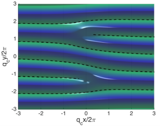
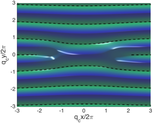
Figure 1: Dislocation pairs in the stripe phase. The dislocations are centered at $(x_{1},y_{1})$ and $(x_{2},y_{2})$ so that the phase field is $u({\bf r})=\arctan[(y-y_{1})/(x-x_{1})]-\arctan[(y-y_{2})/(x-x_{2})]$. Top: A $Q=1$ dislocation centered at $(0,-2.7\pi/q_{c})$ and a $Q=-1$ dislocation centered at $(0,2.7\pi/q_{c})$. Bottom: A $Q=1$ dislocation centered at $(-3\pi/q_{c},0)$ and a $Q=-1$ dislocation centered at $(3\pi/q_{c},0)$. The dashed lines indicate the position of the density maxima.

The spontaneous thermal excitation of bound dislocation pairs decreases the elastic coefficients at a macroscopic scale. The softening of the effective stiffness constant $B$ can be calculated from the well-known renormalisation group equations as described in the methods section. At a critical temperature $T_{c}^{\text{st}}$, the renormalised elastic coefficient $B_{R}$ drops to zero by a sudden jump of magnitude $2T_{c}^{\text{st}}/\pi$. This disappearance of elastic rigidity signals the melting of the density stripes.

I.3 Calculation of bare stiffness constants

We now turn to a microscopic calculation of the “bare” stiffness constants $B_{\parallel}$ and $B_{\perp}$ unrenormalised by dislocation pairs. The relevant thermodynamic quantity is the free energy of the system $F({\bf q})$, which depends on the stripe wave vector ${\bf q}$. Any non-uniform phase fluctuation increases the free energy by an amount given by (2) for long wave lengths. To extract the elastic coefficients $B_{\perp}$ and $B_{\parallel}$, we consider two specific distortions: an infinitesimal rotation and an infinitesimal compression/expansion of the stripes away from the equilibrium configuration, as illustrated in Fig. 2.

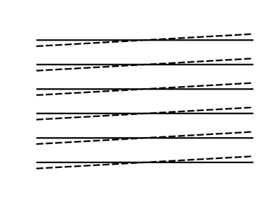
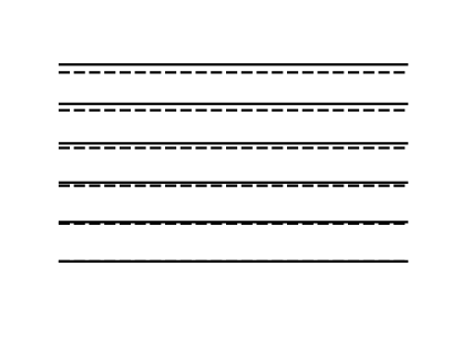
Figure 2: Elementary distortions of the stripes. Rotation (left) and compression (right) of the stripes away from their equilibrium positions indicated by the solid lines.

These distortions are described by the phase field $u({\mathbf{r}})=-\delta{\mathbf{q}}\cdot{\mathbf{r}}$, where $\delta{\mathbf{q}}=\delta q_{\parallel}\cdot\mathbf{e}_{y}$ for the compression and $\delta{\mathbf{q}}=\delta q_{\perp}\cdot\mathbf{e}_{x}$ for the rotation. They are thus equivalent to a variation of the stripe vector ${\mathbf{q}}={\mathbf{q}}_{c}+\delta{\mathbf{q}}$. Inserting the phase fluctuations into Eq. (2), we obtain the increment of the free energy

$$F_{\rm el}=F({\bf q}_{c}+\delta{\bf q})-F({\bf q}_{c})=\frac{A}{2}(B_{\perp}\delta q_{\perp}^{2}+B_{\parallel}\delta q_{\parallel}^{2}),$$ (3)

where $A$ is the area of the system, and we have used the equilibrium condition $\nabla F({\bf q})|_{{\bf q}_{c}}=0$. We thus find

$$B_{\perp}=\frac{1}{A}\left.\frac{\partial^{2}F({\bf q})}{\partial q_{\perp}^{2}}\right|_{{\bf q}_{c}},\quad B_{\parallel}=\frac{1}{A}\left.\frac{\partial^{2}F({\bf q})}{\partial q_{\parallel}^{2}}\right|_{{\bf q}_{c}}.$$ (4)

The interaction energy per particle due to stripe formation scales as $D^{2}n_{0}^{-3/2}(n_{1}/n_{0})^{2}$. Assuming that the interaction energy is dominant, we find that the elastic coefficient $B$ scales as $\sim(n_{1}/n_{0})^{2}g\epsilon_{F}$ for a fixed $\Theta$. The magnitude of $B$ can be further reduced by a geometrical factor depending on $\Theta$, since the system becomes rotationally symmetric for $\Theta=0$, as we shall discuss below.

In order to microscopically calculate the bare stiffness constants, we employ Hartree-Fock mean-field theory for the free energy, writing $F({\bf q})\simeq F_{\text{MF}}({\bf q})=\Omega_{\text{MF}}+\mu N$, where $\Omega_{\text{MF}}$ is the mean-field thermodynamic potential given by

$$\Omega_{\text{MF}}=-E_{\rm int}-T\sum_{j,\bar{\bf k}}\ln\left[1+e^{-\beta\left(\varepsilon_{j\bar{\bf k}}-\mu\right)}\right],$$ (5)

$\mu$ is the chemical potential and $N$ is the total number of particles. The quasiparticle energies are $\varepsilon_{j\bar{\bf k}}$, where $j=1,2,\cdots$ is the band index and $\bar{\bf k}$ is restricted to the first Brillouin zone of the 1D periodic potential set up by the stripes. We subtract the interaction energy $E_{\rm int}$ to avoid double counting. The details of this calculation are given in the methods section.

In Fig. 3, we plot the bare elastic coefficients obtained from this approach as a function of temperature for $g=1$ and $\Theta=0.28\pi$, for which the system has a large stripe amplitude $n_{1}/n_{0}\simeq 0.6$ at low temperatures. In order to minimize finite size effects, we determine the elastic coefficients by fitting a parabolic curve to the free energy in the vicinity of ${\bf q}={\bf q}_{c}$ in accordance with (3), instead of performing a numerical differentiation following (4). This is illustrated in the insets of Fig. 3. This procedure allows us to obtain numerically accurate values for the elastic coefficients. From Fig. 3, we see that both elastic coefficients decrease with increased temperature. This is expected since thermal excitations of quasi-particles reduce the stripe amplitude and thus their rigidity. We also find that $B_{\perp}\ll B_{\parallel}$, which suggests that compressing/expanding the stripes costs more energy than a rotation. This difference in magnitude becomes even more profound for small $\Theta$ when $B_{\perp}$ is strongly suppressed by the weak anisotropy of the system. Finally we note that for $g=1$ and $\Theta=0.28\pi$, the system is in fact predicted to have additional superfluid pairing at $T=0$ Wu et al. (2015). However, as demonstrated in Ref. Wu et al. (2015), the superfluid order has negligible effects on the stripe formation, and it can thus be safely neglected when analysing the elastic properties of the stripes.

Figure 3: Bare stiffness constants as a function of temperature. Upper curve gives $B_{\parallel}$ and lower curve $B_{\perp}$ for $g=1$ and $\Theta=0.28\pi$. The blue circles in the insets are elastic free energy plotted as a function of ${\bf q}$ at $T=0.01\epsilon_{F}$, and the red solid curves are parabolic fits to several data points in the vicinity of ${\bf q}={\bf q}_{c}$.

In Fig. 4, we plot the bare elastic constants as a function of the tilting angle $\Theta$ for $g=1$ and $T=0.01\epsilon_{F}$. The elastic constant $B_{\parallel}$ depends non-monotonically on $\Theta$, first decreasing and then increasing exhibiting a minimum at $\Theta\simeq 0.24\pi$. This is consistent with the mean-field phase diagram, which shows that the stripe formation is somewhat suppressed for intermediate values of $\Theta$ Block and Bruun (2014); Wu et al. (2015). To illustrate this, we plot as an inset the stripe amplitude $n_{1}$ as a function of $\Theta$; we see that it exhibits the same non-monotonic behaviour as $B_{\parallel}$. In comparison to this behaviour, Fig. 4 shows that $B_{\perp}$ increases monotonically in $\Theta$. In particular, we have $B_{\perp}\rightarrow 0$ for $\Theta\rightarrow 0$ as shown in detail in the inset. This reflects that the system is rotationally symmetric for $\Theta=0$ such that a rotation of the stripes costs no energy.

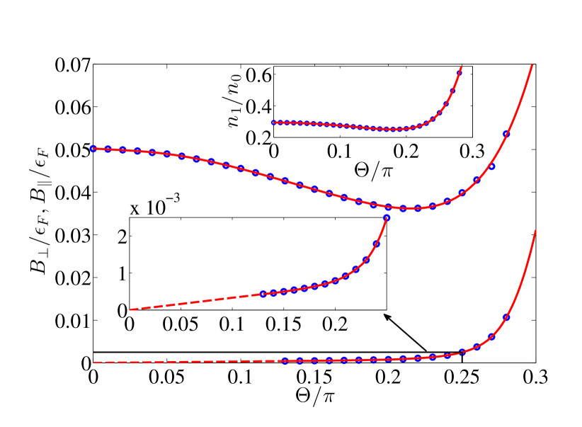
Figure 4: Bare stiffness constants as a function of tilting angle. Upper curve gives $B_{\parallel}$ and lower curve $B_{\perp}$ for $g=1$ and $T=0.01\epsilon_{F}$. For $B_{\perp}$, the red dashed line is an extrapolation for $\Theta<0.13\pi$, where the coefficient is too small to be accurately determined with our numerical method. The upper inset is a plot of the relative stripe amplitude as a function of $\Theta$. The lower inset is an expanded view of the $B_{\perp}$ for small values of $\Theta$.

I.4 Renormalised stiffness constants and stripe melting

The bare elastic constants obtained from the mean-field theory can now be used as initial values in the RG equations to determined the renormalised elastic constants. We also need the dislocation core energy, which must scale as $\sim B$. Therefore, we write $E_{c}=\kappa B$, where $\kappa$ is a constant of order unity. In Fig. 5, we plot the renormalised elastic coefficient $B_{R}$ as a function of temperature, obtained by solving (9) with the initial mean-field values of $B=\sqrt{B_{\perp}B_{\parallel}}$ and $E_{c}=\kappa B$ for various coupling strengths $g$ and tilting angles $\Theta$. To examine the dependence on the core energy, we have chosen different values of $\kappa$. We see that the thermal excitation of dislocation pairs soften the elastic coefficients as expected. This softening is negligible for low $T$ where the core energy prohibits the excitation of dislocations. The softening increases with decreasing core energy and increasing $T$. At the critical temperature $T_{c}^{\text{st}}$ determined by the solution to $2T/\pi=B_{R}(T)$, the elastic coefficient drops to zero discontinuously and the stripes melt.

Figure 5: Renormalised stiffness constants as a function of temperature. The three groups of curves for $B_{R}(T)$ for $g=1$ correspond to, in the order from bottom to up, $\Theta=0.2\pi$, $\Theta=0.26\pi$ and $\Theta=0.28\pi$ respectively. In each of the group, the four curves, in the order from bottom to up, correspond to $\kappa=2,3,4$ and $\infty$ (mean-field result) respectively. The slope of the dashed diagonal line is $2/\pi$.

The resulting melting temperature $T_{c}^{\text{st}}$ is plotted in Fig. 6 as a function of $\Theta$ for $g=1$ and $\kappa=3$. It increases rapidly with $\Theta$, indicating that the degree of anisotropy of the system increases such that the stripes become more rigid. An extrapolation of our calculation for $g=1$ and $\kappa=3$ shows that $T_{c}^{\text{st}}\sim 0.06\epsilon_{F}$ for $\Theta\simeq 0.3\pi$. The critical temperature also increases with the coupling strength, scaling as $T_{c}^{\text{st}}\sim B\sim(n_{1}/n_{0})^{2}g\epsilon_{F}^{0}$. We note that in addition to the explicit linear dependence on $g$, the $T_{c}^{\text{st}}$ can further increase with the coupling strength through the dependence on $n_{1}$. Our results show that in order to observe the stripe phase and the associated BKT physics with dipoles, it is preferable to choose a large tilting angle in addition to having a large dipole moment. However, the tilting angle cannot exceed $\Theta\simeq 0.3\pi$ above which the system exhibits a density collapse for large coupling strengths Bruun and Taylor (2008); Wu et al. (2015).

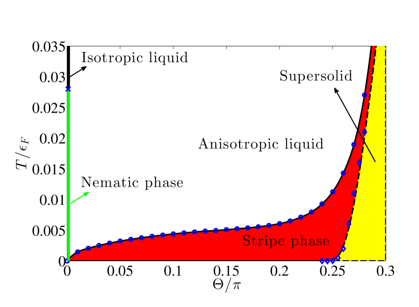
Figure 6: Phase diagram for $g=1$. The system is in the stripe phase below the Kosterlitz-Thouless melting temperature which is calculated taking $\kappa=3$ for the core energy. For $\Theta=0$, the striped phase melts at $T=0_{+}$ into a nematic phase with long range orientational order but no translational order. The nematic phase melts into an isotropic liquid at a temperature $T_{c}^{\text{n}}\simeq B_{\parallel}$ indicated by the blue cross. For $\Theta\gtrsim\arcsin(2/3)$ the system is in a supersolid phase at $T=0$ with both stripe and superfluid order. The transition temperatures of this phase calculated for various tilting angles are indicated by the diamonds. The dashed curve is a fit to the data by (7).

I.5 Melting of supersolid phase

The system exhibits $p$-wave pairing for $\Theta>\arcsin(2/3)$ Bruun and Taylor (2008), which can coexist with stripe order for $g>g_{c}(\Theta)$ at $T=0$ Wu et al. (2015). We now determine the critical temperature $T_{c}^{\text{sf}}$ for the superfluid transition. The 2D superfluid transition is in principle also determined by the BKT mechanism, where the topological defects are now vortices. For weak pairing, however, the mean-field BCS theory in fact gives a good estimate of the transition temperature. We thus determine the critical temperature by solving the linearised gap equation

$$\Delta_{\bf k}=-\int\frac{d{\bf k}^{\prime}}{(2\pi)^{2}}\mathcal{V}({\bf k},-{\bf k}^{\prime})\Delta_{{\bf k}^{\prime}}\left[\frac{\tanh(\xi_{{\bf k}^{\prime}}/2T)}{2\xi_{{\bf k}^{\prime}}}-\frac{\mathcal{P}}{2\xi_{{\bf k}^{\prime}}}\right].$$ (6)

Here $\Delta_{\bf k}$ is the gap parameter and $\mathcal{V}({\bf k},-{\bf k}^{\prime})$ is the effective interaction between the quasiparticles in the stripe phase with energy dispersion $\xi_{\bf k}$ measured from the Fermi surface. The details of this calculation are given in the methods section. The critical temperature obtained from this calculation is shown in Fig. 6 for $g=1$ and for several tilting angles. This mean-field result gives an upper bound to the critical temperature, but since $T_{c}^{\text{sf}}\ll\epsilon_{F}$ we expect that a more detailed BKT calculation yield only slightly smaller values. This should be contrasted with the melting of the stripes, where an estimate of the critical temperature from a vanishing stripe order would give a much higher value compared to the BKT calculation. This can be seen from Fig. 3, which shows that the mean-field elastic coefficients remain large up to $T=0.12\epsilon_{F}$. Thus, it is crucial to use the BKT theory to analyse the stripe melting.

Using a simple $p$-wave ansatz for the gap parameter $\Delta_{\bf k}\simeq\Delta\cos\phi$, where $\phi$ is the polar angle of the wave vector ${\bf k}$, one can obtain an approximate solution for the critical temperature as

$$T_{c}^{\text{sf}}\simeq C\epsilon_{F}e^{-{1}/{\left[g\left(\frac{9}{4}\sin^{2}\Theta-1\right)\right]}},$$ (7)

where C is a constant related to an effective momentum cutoff in the integral in (6). We find that the data obtained from solving (6) numerically are in fact very well described by (7) with $C\simeq 0.4$.

I.6 Quantum nematic phase for $\Theta=0$

Figure 6 shows that the critical temperature for the stripe phase vanishes as $\Theta\rightarrow 0$. This is a direct consequence of the rotational symmetry rendering $B_{\perp}=0$ for $\Theta=0$. In this case, the system is no longer described by the XY model. Instead, an appropriate expression for the elastic energy of stripe fluctuations is Toner and Nelson (1981)

$$F_{\rm el}=\frac{1}{2}B_{\parallel}\int d^{2}r[\lambda^{2}(\partial_{x}^{2}u)^{2}+(\partial_{y}u)^{2}],$$ (8)

where $\lambda$ is a length comparable to the stripe spacing. Dislocations again play an important role in determining the finite temperature properties of the system described by (8). In contrast to the $\Theta>0$ case, however, single dislocations now have a finite energy and can be thermally excited. When the presence of the free dislocations is taken into account, a system described by (8) is predicted to be in a nematic phase for $0<T<T_{c}^{\text{n}}$, and in an isotropic liquid phase for $T>T_{c}^{n}$ Toner and Nelson (1981). In the nematic phase, the translational order exists only within a length scale $\xi_{D}$, which is determined by the density of the free dislocations. The stripe orientations, averaged over the length scale $\xi_{D}$, are however algebraically correlated. As a crude physical picture, one can think of the nematic phase as blobs of stripe order of area $\sim\xi_{D}^{2}$, which are all oriented more or less in the same direction, but which are not positionally correlated with each other. The nematic phase is in this sense analogous to the 2D hexatic phase of a crystal, which exhibits bond orientational order but no long-range translational order Halperin and Nelson (1978); Nelson and Halperin (1979); Nelson (2002). A quantum hexatic phase was recently predicted to exist in 2D dipolar gases for very strong coupling $g\gtrsim 27$ Bruun and Nelson (2014); Lechner et al. (2014). The results presented here point out the intriguing possibility to realise a quantum version of the nematic phase with dipoles for smaller coupling strengths. We expect the critical temperature $T_{c}^{\text{n}}$ for the melting of the quantum nematic phase to scale as $B_{\parallel}$. However, a quantitative calculation of the critical temperature for the dipolar system requires knowledge of the parameter $\lambda$, whose determination is beyond our current theoretical framework. In Fig. 6, we have indicated the critical temperature $T_{c}^{n}$ using a somewhat smaller value than the bare $B_{\parallel}$ due to renormalisation effects.

II Discussion

An important question concerns whether the critical temperature for the predicted quantum liquid crystal phases is within experimental reach. As an example, let us consider a recent experiment reporting the trapping of chemically stable ²³Na⁴⁰K molecules in their ground state close to quantum degeneracy. The group obtained an induced dipole moment of $d=0.8$Debye and a maximum 3D density of $n_{\text{3D}}=2.5\times 10^{11}$cm^-3 Park et al. (2015). Estimating a corresponding 2D areal density as $n_{0}=n_{\text{3D}}^{2/3}$, these values correspond to $g\simeq 0.57$. This coupling strength can be increased by reaching a larger fraction of the permanent electric dipole moment of ²³Na⁴⁰K, which is $2.72$Debye Gerdes, A. et al. (2011), or by increasing the density of the gas. Since the critical temperature for the nematic and the stripe phases both scale as $\sim(n_{1}/n_{0})^{2}g\epsilon_{F}$, this indicates that the quantum liquid crystal physics discussed in this paper is within experimental reach, once dipolar gases can be cooled down significantly below their Fermi temperature.

The formation of stripe and superfluid order can be observed as correlation peaks in time-of-flight (TOF) experiments Block and Bruun (2014); Wu et al. (2015). One can also detect the stripes directly as density modulations, either after TOF or in-situ, provided that the experimental resolution is sufficiently high. Observing the proliferation of dislocations would directly confirm the microscopic mechanism behind the BKT transition.

Finally, we would like to mention a recent fixed note Monte-Carlo calculation which suggests that the striped phase is not the ground state for $\Theta=0$ for any coupling strength Matveeva and Giorgini (2012). We speculate that this result, which contradicts that of Refs. Yamaguchi et al. (2010); Babadi and Demler (2011); Sieberer and Baranov (2011); Block et al. (2012); Block and Bruun (2014); van Zyl et al. (2015); Parish and Marchetti (2012), is due to the approximate nature of the calculation combined with the fragility of the striped phase, which melts at any non-zero temperature for $\Theta=0$, as shown by our results.

In summary, we analysed the phase diagram of a 2D dipolar gases, which exhibits stripe, nematic and supersolid phases corresponding to the breaking of translational, rotational and gauge symmetry. For a non-zero tilting angle $\Theta$, the low energy degrees of freedom of the striped phase are described by an anisotropic 2D XY model. We calculated the stiffness constants corresponding to a rotation and a compression/expansion of the stripes microscopically. This should be contrasted with electron systems, where such stiffness constants are often simply unknown parameters of the theory. The stripes were shown to melt via the Berezinskii-Kosterlitz-Thouless mechanism due to the proliferation of dislocations, and we obtained the melting temperature using the relevant renormalisation group equations. We also calculated the critical temperature of the supersolid phase. For $\Theta=0$, the striped phase is stable only at $T=0$, which melts into a nematic phase for arbitrarily small temperatures. Our analysis of the melting temperatures demonstrated that they should be within experimental reach. An observation of these phases would constitute a major breakthrough in our understanding of the interplay between liquid crystal and superfluid order in low-dimensional many-body systems.

III Methods

III.1 Renormalisation group equations

We calculate the softening of the effective stiffness constant $B=\sqrt{B_{\parallel}B_{\perp}}$ due to the excitations of dislocation pairs using the well-known renormalisation group equations

$$\frac{dK^{-1}(l)}{dl}=2\pi^{3}y^{2}(l)$$

$$\frac{dy(l)}{dl}=[2-\pi K(l)]y(l).$$ (9)

Here $K(l)=B(l)/T$ and $y(l)=\exp[-E_{c}(l)/T]$ are the scale-dependent stiffness constant and dislocation fugacity respectively. They both decrease with increasing $l$ as the renormalisation due to dislocation pairs at larger length scales are included via the solution of (9). The initial values of $K(0)$ and $y(0)$ are the bare (local) values unrenormalised by dislocation pairs, which we calculate microscopically as described in the text. At a critical temperature $T_{c}^{\text{st}}$, the long range renormalised elastic coefficient $B_{R}\equiv\lim_{l\rightarrow\infty}B(l)$ drops to zero by a sudden jump of $2T_{c}^{\text{st}}/\pi$. This disappearance of elastic rigidity signals the melting of the stripes.

III.2 Mean-field theory of stripe formation

The mean-field Hamiltonian that takes into account the possibility of stripe formation with a wave vector ${\bf q}$ is given by Block and Bruun (2014)

$$\hat{\mathcal{H}}_{MF}=\sum_{{\bf k}}\epsilon_{\bf k}\hat{c}_{\bf k}^{\dagger}\hat{c}_{\bf k}+\sum_{\bf k}[h_{\bf k}\hat{c}^{\dagger}_{{\bf k}+{\bf q}}\hat{c}_{\bf k}+h.c.],$$ (10)

where $\hat{c}_{\bf k}^{\dagger}$ creates a dipole with momentum ${\bf k}$, $\epsilon_{\bf k}$ is the single particle Hartree-Fock energy

$$\epsilon_{\bf k}=\frac{k^{2}}{2m}+\frac{1}{A}\sum_{{\bf k}^{\prime}}[V(0)-V({\bf k}-{\bf k}^{\prime})]\langle\hat{c}_{{\bf k}^{\prime}}^{\dagger}\hat{c}_{{\bf k}^{\prime}}\rangle,$$ (11)

and $h_{\bf k}$ is a real off-diagonal element defined by

$$h_{\bf k}=\frac{1}{A}\sum_{{\bf k}^{\prime}}[V({\bf q})-V({\bf k}-{\bf k}^{\prime})]\langle\hat{c}^{\dagger}_{{\bf k}^{\prime}}\hat{c}_{{\bf k}^{\prime}+{\bf q}}\rangle.$$ (12)

The quasi-2D interaction in Fourier space is obtained by averaging the interaction over the harmonic oscillator ground state in the $z$ direction. This gives (up to an irrelevant constant term) Fischer (2006)

$$V({\bf k}) \simeq-g\frac{3\pi^{2}k}{2mk^{0}_{F}}\left(\cos^{2}\Theta-\sin^{2}\Theta\cos^{2}\varphi\right),$$ (13)

where $\varphi$ is the polar angle of ${\bf k}$. We diagonalise the mean-field Hamiltonian by generalising the method described in Refs. Block and Bruun (2014); Wu et al. (2015) to an arbitrary stripe vector ${\bf q}$. This yields the Hamiltonian

$$\hat{\mathcal{H}}_{MF}=\sum_{j\bar{\bf k}}\varepsilon_{j\bar{\bf k}}\hat{\gamma}^{\dagger}_{j\bar{\bf k}}\hat{\gamma}_{j\bar{\bf k}}.$$ (14)

Here $\hat{\gamma}_{j\bar{\bf k}}=\sum_{\bf G}U_{j,\bar{\bf k}+{\bf G}}\hat{c}_{\bar{\bf k}+{\bf G}}$ annihilates a quasiparticle with energy $\varepsilon_{j\bar{\bf k}}$, where $j=1,2,\cdots$ is the band index, ${\bf G}=l{\bf q},l=0,\pm 1,\cdots$ is the reciprocal lattice vector and $\bar{\bf k}$ is restricted to the first Brillouin zone of the 1D periodic potential set up by the stripes. We can then calculate the mean-field free energy as $F_{\text{MF}}({\bf q})=\Omega_{\text{MF}}+\mu N$, where $\Omega_{\text{MF}}$ is the mean-field thermodynamic potential given by (5) and $N=\sum_{j,\bar{\bf k}}f_{j\bar{\bf k}}$ with $f_{j\bar{\bf k}}=[\exp\beta(\varepsilon_{j\bar{\bf k}}-\mu)+1]^{-1}$. The interaction energy is most easily calculated using

$$E_{\text{MF}}=\sum_{j,\bar{\bf k}}\varepsilon_{j\bar{\bf k}}f_{j\bar{\bf k}}=E_{\text{kin}}+2E_{\text{int}}$$ (15)

where $E_{\text{kin}}=\sum_{\bf k}\langle\hat{c}^{\dagger}_{\bf k}\hat{c}_{\bf k}\rangle k^{2}/2m$ the kinetic energy.

III.3 BCS theory of the superfluid transition

To explore superfluid pairing within the stripe phase, we use BCS theory with the quasiparticle Hamiltonian $\hat{\mathcal{H}}_{\rm BCS}=\hat{\mathcal{H}}_{\rm MF}+\hat{\mathcal{H}}_{\rm P}$. Here,

$$\hat{\mathcal{H}}_{\rm P}=\sum_{{jj^{\prime}\bar{\bf k}\bar{\bf k}^{\prime}}}\frac{\mathcal{V}_{j^{\prime}j}(\bar{\bf k}^{\prime},-\bar{\bf k})}{2}\langle\hat{\gamma}^{\dagger}_{j^{\prime}\bar{\bf k}^{\prime}}\hat{\gamma}_{j^{\prime},-\bar{\bf k}^{\prime}}^{\dagger}\rangle\hat{\gamma}_{j\bar{\bf k}}\hat{\gamma}_{j,-\bar{\bf k}}+\rm{h.c.}$$

describes pairing between the time-reversed quasiparticles, interacting via

$$\mathcal{V}_{j^{\prime}j}(\bar{\bf k}^{\prime},-\bar{\bf k})=\sum_{{\bf G}{\bf G}^{\prime}\tilde{\bf G}\tilde{\bf G}^{\prime}}\delta_{{\bf G}-{\bf G}^{\prime},\tilde{\bf G}^{\prime}-\tilde{\bf G}}U^{*}_{j^{\prime},\bar{\bf k}^{\prime}+{\bf G}^{\prime}}U^{*}_{j^{\prime},-\bar{\bf k}^{\prime}+\tilde{\bf G}^{\prime}}$$

$$\times U_{j,-\bar{\bf k}+\tilde{\bf G}}U_{j,\bar{\bf k}+{\bf G}}V\left(\bar{\bf k}-\bar{\bf k}^{\prime}+{\bf G}-{\bf G}^{\prime}\right).$$ (16)

To derive a gap equation that is amenable to a partial wave expansion, we switch to the “extended zone scheme”, whereby a single particle state $\psi_{j\bar{\bf k}}({\bm{\rho}})$ in the $j$’th band in the first BZ is mapped onto a state $\psi_{{\bf k}}({\bm{\rho}})$ in the $j$’th BZ in the standard way Wu et al. (2015), where the vector ${\bf k}$ is now unrestricted. The effective pairing interaction $\mathcal{V}_{j^{\prime}j}(\bar{\bf k}^{\prime},-\bar{\bf k})$ shall be denoted by $\mathcal{V}({\bf k},-{\bf k}^{\prime})$ and quasi-particle dispersion $\varepsilon_{j\bar{\bf k}}$ by $\varepsilon_{\bf k}$. Pairing between time-reversed quasiparticles gives rise to the gap parameter $\Delta_{{\bf k}}\equiv\sum_{{\bf k}^{\prime}}\mathcal{V}({\bf k},-{\bf k}^{\prime})\langle\hat{\gamma}_{-{\bf k}^{\prime}}\hat{\gamma}_{{\bf k}^{\prime}}\rangle$, which satisfies the finite temperature gap equation

$$\Delta_{\bf k}=-\int\frac{d{\bf k}^{\prime}}{(2\pi)^{2}}\mathcal{V}({\bf k},-{\bf k}^{\prime})\Delta_{{\bf k}^{\prime}}\left[\frac{\tanh(E_{{\bf k}^{\prime}}/2T)}{2E_{{\bf k}^{\prime}}}-\frac{\mathcal{P}}{2\xi_{{\bf k}^{\prime}}}\right].$$ (17)

Here $\xi_{\bf k}=\varepsilon_{\bf k}-\mu$ and $E_{\bf k}=\sqrt{\xi_{{\bf k}}^{2}+|\Delta_{\bf k}|^{2}}$, where the chemical potential $\mu$ is approximated by the value in the stripe phase. The Cauchy principal value term $\mathcal{P}/2\xi_{{\bf k}^{\prime}}$ in (17) renders the gap equation well defined with no need for a high momentum cut-off. At temperatures in the vicinity of the superfluid transition, the linearisation of the above gap equation yields (6) we use in the main text. Equation (6) can be solved by the method of partial wave expansion described in Ref. Wu et al. (2015). Finally we determine the transition temperature by gradually increasing $T$ in the gap equation until it ceases to admit finite solutions.

IV Acknowledgement

G.M.B. would like to acknowledge the support of the Hartmann Foundation via grant A21352 and the Villum Foundation via grant VKR023163.

V Additional information

Competing financial interests: The authors declare no competing financial interests.

References

- Baranov (2008) M. Baranov, Physics Reports 464, 71 (2008).
- Lahaye et al. (2009) T. Lahaye, C. Menotti, L. Santos, M. Lewenstein, and T. Pfau, Reports on Progress in Physics 72, 126401 (2009).
- Lu et al. (2012) M. Lu, N. Q. Burdick, and B. L. Lev, Phys. Rev. Lett. 108, 215301 (2012).
- Aikawa et al. (2014) K. Aikawa, A. Frisch, M. Mark, S. Baier, R. Grimm, J. L. Bohn, D. S. Jin, G. M. Bruun, and F. Ferlaino, Phys. Rev. Lett. 113, 263201 (2014).
- Heo et al. (2012) M.-S. Heo, T. T. Wang, C. A. Christensen, T. M. Rvachov, D. A. Cotta, J.-H. Choi, Y.-R. Lee, and W. Ketterle, Phys. Rev. A 86, 021602 (2012).
- Park et al. (2015) J. W. Park, S. A. Will, and M. W. Zwierlein, Phys. Rev. Lett. 114, 205302 (2015).
- Fradkin and Kivelson (2010) E. Fradkin and S. A. Kivelson, Science 327, 155 (2010), http://www.sciencemag.org/content/327/5962/155.full.pdf .
- Kivelson et al. (1998) S. A. Kivelson, E. Fradkin, and V. J. Emery, Nature 393, 550 (1998).
- Chuang et al. (2010) T.-M. Chuang, M. P. Allan, J. Lee, Y. Xie, N. Ni, S. L. Bud’ko, G. S. Boebinger, P. C. Canfield, and J. C. Davis, Science 327, 181 (2010), http://www.sciencemag.org/content/327/5962/181.full.pdf .
- Emery et al. (1999) V. J. Emery, S. A. Kivelson, and J. M. Tranquada, Proceedings of the National Academy of Sciences 96, 8814 (1999), http://www.pnas.org/content/96/16/8814.full.pdf .
- Kohsaka et al. (2007) Y. Kohsaka, C. Taylor, K. Fujita, A. Schmidt, C. Lupien, T. Hanaguri, M. Azuma, M. Takano, H. Eisaki, H. Takagi, S. Uchida, and J. C. Davis, Science 315, 1380 (2007), http://www.sciencemag.org/content/315/5817/1380.full.pdf .
- Hadzibabic et al. (2006) Z. Hadzibabic, P. Kruger, M. Cheneau, B. Battelier, and J. Dalibard, Nature 441, 1118 (2006).
- Bishop and Reppy (1978) D. J. Bishop and J. D. Reppy, Phys. Rev. Lett. 40, 1727 (1978).
- Fiory et al. (1983) A. T. Fiory, A. F. Hebard, and W. I. Glaberson, Phys. Rev. B 28, 5075 (1983).
- Reyren et al. (2007) N. Reyren, S. Thiel, A. D. Caviglia, L. F. Kourkoutis, G. Hammerl, C. Richter, C. W. Schneider, T. Kopp, A.-S. Rüetschi, D. Jaccard, M. Gabay, D. A. Muller, J.-M. Triscone, and J. Mannhart, Science 317, 1196 (2007), http://www.sciencemag.org/content/317/5842/1196.full.pdf .
- Ye et al. (2010) J. T. Ye, S. Inoue, K. Kobayashi, Y. Kasahara, H. T. Yuan, H. Shimotani, and Y. Iwasa, Nat Mater 9, 125 (2010).
- Matthey et al. (2007) D. Matthey, N. Reyren, J.-M. Triscone, and T. Schneider, Phys. Rev. Lett. 98, 057002 (2007).
- Rout and Budhani (2010) P. K. Rout and R. C. Budhani, Phys. Rev. B 82, 024518 (2010).
- Resnick et al. (1981) D. J. Resnick, J. C. Garland, J. T. Boyd, S. Shoemaker, and R. S. Newrock, Phys. Rev. Lett. 47, 1542 (1981).
- Safonov et al. (1998) A. I. Safonov, S. A. Vasilyev, I. S. Yasnikov, I. I. Lukashevich, and S. Jaakkola, Phys. Rev. Lett. 81, 4545 (1998).
- Yamaguchi et al. (2010) Y. Yamaguchi, T. Sogo, T. Ito, and T. Miyakawa, Phys. Rev. A 82, 013643 (2010).
- Babadi and Demler (2011) M. Babadi and E. Demler, Phys. Rev. B 84, 235124 (2011).
- Sieberer and Baranov (2011) L. M. Sieberer and M. A. Baranov, Phys. Rev. A 84, 063633 (2011).
- Block et al. (2012) J. K. Block, N. T. Zinner, and G. M. Bruun, New Journal of Physics 14, 105006 (2012).
- Block and Bruun (2014) J. K. Block and G. M. Bruun, Phys. Rev. B 90, 155102 (2014).
- van Zyl et al. (2015) B. P. van Zyl and W. Kirkby, and W. Ferguson, Phys. Rev. A 92, 023614 (2015).
- Parish and Marchetti (2012) M. M. Parish and F. M. Marchetti, Phys. Rev. Lett. 108, 145304 (2012).
- Bruun and Taylor (2008) G. M. Bruun and E. Taylor, Phys. Rev. Lett. 101, 245301 (2008).
- Astrakharchik et al. (2007) G. E. Astrakharchik, J. Boronat, I. L. Kurbakov, and Y. E. Lozovik, Phys. Rev. Lett. 98, 060405 (2007).
- Büchler et al. (2007) H. P. Büchler, E. Demler, M. Lukin, A. Micheli, N. Prokof’ev, G. Pupillo, and P. Zoller, Phys. Rev. Lett. 98, 060404 (2007).
- Chaikin and Lubensky (2000) P. Chaikin and T. Lubensky, Principles of Condensed Matter Physics (Cambridge University Press, 2000).
- Nelson (2002) D. R. Nelson, Defects and Geometry in Condensed Matter Physics (Cambridge University Press, Cambridge, 2002).
- Berezinskii (1972) V. L. Berezinskii, Soviet Physics JETP 34, 610 (1972).
- Kosterlitz and Thouless (1973) J. M. Kosterlitz and D. J. Thouless, Journal of Physics C: Solid State Physics 6, 1181 (1973).
- Kosterlitz (1974) J. M. Kosterlitz, Journal of Physics C: Solid State Physics 7, 1046 (1974).
- José et al. (1977) J. V. José, L. P. Kadanoff, S. Kirkpatrick, and D. R. Nelson, Phys. Rev. B 16, 1217 (1977).
- Wu et al. (2015) Z. Wu, J. K. Block, and G. M. Bruun, Phys. Rev. B 91, 224504 (2015).
- Toner and Nelson (1981) J. Toner and D. R. Nelson, Phys. Rev. B 23, 316 (1981).
- Halperin and Nelson (1978) B. I. Halperin and D. R. Nelson, Phys. Rev. Lett. 41, 121 (1978).
- Nelson and Halperin (1979) D. R. Nelson and B. I. Halperin, Phys. Rev. B 19, 2457 (1979).
- Bruun and Nelson (2014) G. M. Bruun and D. R. Nelson, Phys. Rev. B 89, 094112 (2014).
- Lechner et al. (2014) W. Lechner, H.-P. Büchler, and P. Zoller, Phys. Rev. Lett. 112, 255301 (2014).
- Gerdes, A. et al. (2011) Gerdes, A., Dulieu, O., Knöckel, H., and Tiemann, E., Eur. Phys. J. D 65 (2011).
- Matveeva and Giorgini (2012) N. Matveeva and S. Giorgini, Phys. Rev. Lett. 109, 200401 (2012).
- Fischer (2006) U. R. Fischer, Phys. Rev. A 73, 031602 (2006).