Topological superconductor with a large Chern number and a large bulk excitation gap in single layer graphene

Abstract

We show that a two-dimensional topological superconductor (TSC) can be realized in a hybrid system with a conventional $s$-wave superconductor proximity-coupled to a quantum anomalous Hall (QAH) state from the Rashba and exchange effects in single layer graphene. With very low or even zero doping near the Dirac points, i.e., two inequivalent valleys, this TSC has a Chern number as large as four, which supports four Majorana edge modes. More importantly, we show that this TSC has a robust topologically nontrivial bulk excitation gap, which can be larger or even one order of magnitude larger than the proximity-induced superconducting gap. This unique property paves a way for the application of QAH insulators as seed materials to realize robust TSCs and Majorana modes.

I INTRODUCTION

Majorana modes can naturally exist in topological superconductors (TSCs).kitaev ; alicea1 ; beenakker ; hasan ; qi The intrinsic TSC has been predicted to exist in superconducting Sr₂RuO₄ with $p$-wave paring state.ivanov ; mackenzie However, this has not yet been experimentally confirmed. Recently, many efforts have been devoted to design artificial TSCs.fu ; sau ; sau2 ; alicea2 ; lutchyn ; alicea3 ; halperin ; stanescu ; mourik ; yzhou ; bysun ; nadj ; hui ; dumitrescu ; jianli ; qi2 ; jwang ; poyhonen ; jjhe ; tewari ; tewari2 ; mdiez ; wong ; haim ; rontynen ; dutreix ; jianli2 So far, most studies focus on the effective $p$-wave superconductors in hybrid systems with conventional $s$-wave superconductors in proximity to strong topological insulators,fu semiconductors with strong spin-orbit coupling (SOC), sau ; sau2 ; alicea2 ; lutchyn ; alicea3 ; halperin ; stanescu ; mourik ; yzhou ; bysun ; jjhe ; tewari ; tewari2 ; mdiez ; wong ; haim ; dutreix or ferromagnetic atom chains.nadj ; hui ; dumitrescu ; jianli ; poyhonen ; rontynen ; jianli2 Some attention has also been paid to the conventional $s$-wave superconductors coupled to quantum anomalous Hall (QAH) insulators such as topological insulators with magnetic dopants.qi2 ; jwang Among all the above TSCs, multiple spatially overlapping Majorana modes, which greatly benefit the transport properties, can only coexist in one-dimensional (two-dimensional) TSCs belonging to Class BDI poyhonen ; haim ; dumitrescu ; hui ; jianli ; jjhe ; tewari ; tewari2 ; mdiez ; wong (D qi2 ; jwang ; rontynen ; jianli2 ) with integer topological invariant.schnyder In reality, the one-dimensional TSCs in Class BDI can easily reduce to the ones indexed by Class D with zero or one Majorana mode.poyhonen ; haim ; dumitrescu ; hui ; tewari ; tewari2 ; mdiez ; wong As for the two-dimensional TSCs in Class D, the number of the Majorana modes or the Chern number is limited upto two.qi2 ; jwang ; jianli2 More Majorana modes or larger Chern numbers are limited by large chemical potential (i.e., very high doping) and an overall much smaller bulk excitation gap than the proximity-induced superconducting gap.rontynen ; jianli2

In this work, we show that a two-dimensional TSC can be realized in a hybrid system with a conventional $s$-wave superconductor proximity-coupled to a QAH state qiao due to the Rashba SOC Rashba and exchange field in single layer graphene. Interestingly, with very low or even zero doping near the Dirac points, i.e., two inequivalent valleys, the TSC from the QAH state has a Chern number reaching as large as four, hosting four Majorana edge modes. More importantly, these Majorana modes are protected by a bulk excitation gap, which can be larger or even one order of magnitude larger than the superconducting gap from the proximity effect. This is in strong contrast to the case of effective $p$-wave superconductors where the excitation gap is always smaller than the superconducting gap.sau ; sau2 ; alicea2 ; lutchyn ; alicea3 ; halperin ; stanescu ; mourik ; yzhou ; bysun As the large topologically nontrivial gap has been shown to be probably most important for applications in topological insulators,hasan ; qi topological crystalline insulators,cniu and QAH insulators,cniu ; qiao2 ; gangxu our finding, i.e., reporting a large bulk excitation gap in the TSC is crucial to the field of TSCs and Majorana modes. This paves a way to obtain robust TSCs and Majorana modes using the QAH states. We also address the experimental feasibility of the TSC from the QAH state.

This paper is organized as follows. In Sec. II, we present our model and lay out the tight-binding Hamiltonian of single layer graphene. Then, we calculate the topological invariant in Sec. III. We further presents the results on the phase diagram, Majorana edge states and bulk excitation gap in Sec. IV. Finally, we summarize and discuss in Sec. V.

II MODEL AND HAMILTONIAN

The real-space tight-binding Hamiltonian of single layer graphene with the Rashba SOC, exchange field and proximity-induced $s$-wave superconductivity is given by qiao ; kane ; ezawa

$$H = -t\sum_{\langle i,j\rangle\alpha}c^{\dagger}_{i\alpha}c_{j\alpha}+i\lambda\sum_{\langle i,j\rangle\alpha\beta}{({\mbox{\boldmath$\sigma$\unboldmath}}^{\alpha\beta}\times{\bf d}_{ij})}_{z}c^{\dagger}_{i\alpha}c_{j\beta}$$ (1)

$$\mbox{}-\mu\sum_{i\alpha}c^{\dagger}_{i\alpha}c_{i\alpha}+V_{z}\sum_{i\alpha}c^{\dagger}_{i\alpha}\sigma_{z}^{\alpha\alpha}c_{i\alpha}$$

$$\mbox{}+\Delta\sum_{i}(c^{\dagger}_{i\uparrow}c^{\dagger}_{i\downarrow}+{\rm H.c.}),$$

where $\langle i,j\rangle$ represents the nearest-neighboring sites and $c_{i\alpha}\ (c^{\dagger}_{i\alpha})$ annihilates (creates) an electron with spin $\alpha$ at site $i$. The first term stands for the nearest-neighbor hopping with $t=2.7\$eV neto being the hopping energy. The second term denotes the Rashba SOC with $\lambda$, $\sigma$ and ${\bf d}_{ij}$ representing the coupling strength, Pauli matrices for real spins and a unit vector from site $j$ to site $i$, respectively. $\mu$ in the third term is the chemical potential. $V_{z}$ ($\Delta$) in the fourth (fifth) term corresponds to exchange field (superconducting gap from the proximity effect).

To start, we transform the Hamiltonian of Eq. (1) to the Bogoliubov-de Gennes (BdG) one in the momentum space. Specifically,

$$H=\frac{1}{2}\sum_{\bf k}\Phi^{\dagger}_{\bf k}H_{\rm BdG}({\bf k})\Phi_{\bf k}$$ (2)

where $\Phi^{\dagger}_{\bf k}=(\psi^{\dagger}_{{\rm A}\uparrow}(\bf k),\ \psi^{\dagger}_{{\rm B}\uparrow}(\bf k),\ \psi^{\dagger}_{{\rm A}\downarrow}(\bf k),\ \psi^{\dagger}_{{\rm B}\downarrow}(\bf k),\ \psi_{{\rm A}\downarrow}(-{\bf k}),\\ \psi_{{\rm B}\downarrow}(-{\bf k}),\ -\psi_{{\rm A}\uparrow}(-{\bf k}),\ -\psi_{{\rm B}\uparrow}(-{\bf k}))$ with $\psi^{\dagger}_{i\alpha}({\bf k})$ creating an electron with spin $\alpha$ and momentum ${\bf k}$ counted from the momentum $\Gamma$ at sublattice $i$ ($i={\rm A}$, ${\rm B}$) and

$$H_{\rm BdG}({\bf k})=\left(\begin{array}[]{cc}H_{e}({\bf k})-\mu&\Delta\\ \Delta&\mu-\sigma_{y}H_{e}^{*}(-{\bf k})\sigma_{y}\end{array}\right).$$ (5)

$H_{e}({\bf k})$ represents tight-binding Hamiltonian without the $s$-wave superconductivity, which can be written as

$$H_{e}({\bf k})=\left(\begin{array}[]{cccc}V_{z}&f({\bf k})&0&h_{1}({\bf k})\\ f^{*}({\bf k})&V_{z}&h_{2}^{*}({\bf k})&0\\ 0&h_{2}({\bf k})&-V_{z}&f({\bf k})\\ h_{1}^{*}({\bf k})&0&f^{*}({\bf k})&-V_{z}\end{array}\right)$$ (10)

where $f({\bf k})=-t[(2\cos\frac{k_{x}}{2}\cos\frac{k_{y}}{2\sqrt{3}}+\cos\frac{k_{y}}{\sqrt{3}})-i(2\cos\frac{k_{x}}{2}\sin\frac{k_{y}}{2\sqrt{3}}-\sin\frac{k_{y}}{\sqrt{3}})]$, $h_{1}({\bf k})=-\lambda[(\cos\frac{k_{x}}{2}+\sqrt{3}\sin\frac{k_{x}}{2})\sin\frac{k_{y}}{2\sqrt{3}}+\sin\frac{k_{y}}{\sqrt{3}}]-i\lambda[-\cos\frac{k_{y}}{\sqrt{3}}+\cos\frac{k_{y}}{2\sqrt{3}}(\cos\frac{k_{x}}{2}+\sqrt{3}\sin\frac{k_{x}}{2})]$ and $h_{2}({\bf k})=\lambda[(\sqrt{3}\sin\frac{k_{x}}{2}-\cos\frac{k_{x}}{2})\sin\frac{k_{y}}{2\sqrt{3}}-\sin\frac{k_{y}}{\sqrt{3}}]+i\lambda[\cos\frac{k_{y}}{\sqrt{3}}-\cos\frac{k_{y}}{2\sqrt{3}}(\cos\frac{k_{x}}{2}-\sqrt{3}\sin\frac{k_{x}}{2})]$. Note that the lattice constant is set to be unity in the calculation for simplicity.

III TOPOLOGICAL INVARIANT

Before investigating the topological properties of $H_{\rm BdG}({\bf k})$, we first identify the gap closing conditions. The gap closing of the BdG Hamiltonian $H_{\rm BdG}({\bf k})$ is equivalent to the existence of bulk zero energy states due to particle-hole symmetry. The condition for bulk zero energy states is obtained by calculating ${\rm det}(H_{\rm BdG})=0$. We find that the gap closes at the momenta $\Gamma$ (single one), $M$ (three inequivalent ones) and $K$ (two inequivalent ones) points with the corresponding conditions given by $(\mu\pm 3t)^{2}=V_{z}^{2}-\Delta^{2}$, $(\mu\pm t)^{2}=V_{z}^{2}-\Delta^{2}$ and $\mu^{2}=V_{z}^{2}-\Delta^{2}$, respectively. It is noted that $+$ ($-$) stands for lower (higher) energy band at the momentum $\Gamma$ or $M$. The detailed calculation is shown in Appendix B. Obviously, our system is topologically trivial in the case of $|V_{z}|<|\Delta|$. As for $|V_{z}|\geq|\Delta|$, we have ten critical chemical potentials in order, i.e., $\mu_{1,2}=3t\pm\sqrt{V_{z}^{2}-\Delta^{2}}$, $\mu_{3,4}=t\pm\sqrt{V_{z}^{2}-\Delta^{2}}$, $\mu_{5,6}=\pm\sqrt{V_{z}^{2}-\Delta^{2}}$, $\mu_{7,8}=-t\pm\sqrt{V_{z}^{2}-\Delta^{2}}$, and $\mu_{9,10}=-3t\pm\sqrt{V_{z}^{2}-\Delta^{2}}$ by assuming $|V_{z}|,|\Delta|\ll t$, which divide the system into eleven topological regimes.

These topological regimes are characterized by the Chern number $C_{1}$ since $H_{\rm BdG}(\bf k)$ belongs to Class D with integer topological invariant.schnyder $C_{1}$ can be calculated by ghosh

$$C_{1}=\frac{1}{2\pi}\int_{\rm BZ}d^{2}{\bf k}f_{xy}({\bf k})$$ (11)

with the Berry curvature

$$f_{xy}({\bf k})=i\sum_{m,n}(f_{m}-f_{n}){u_{m}^{\dagger}({\bf k})[\partial_{k_{x}}H_{\rm BdG}({\bf k})]u_{n}({\bf k})}$$

$$\mbox{}\times{u_{n}^{\dagger}({\bf k})[\partial_{k_{y}}H_{\rm BdG}({\bf k})]u_{m}({\bf k})}/{[E_{m}({\bf k})-E_{n}({\bf k})]^{2}}.$$ (12)

Here, $u_{m}({\bf k})$ is the $m$-th eigenvector of $H_{\rm BdG}({\bf k})$ with the corresponding eigenvalue being $E_{m}({\bf k})$; $f_{m}=1\ (0)$ for occupied (empty) band. The Chern number of all topological regimes is given by

$$C_{1}=\left\{\begin{array}[]{ll}1\ (-1),&\mu_{2}<\mu<\mu_{1}\\ -3\ (3),&\mu_{4}<\mu<\mu_{3}\\ 4\ (-4),&\mu_{6}<\mu<\mu_{5}\\ -3\ (3),&\mu_{8}<\mu<\mu_{7}\\ 1\ (-1),&\mu_{10}<\mu<\mu_{9}\\ 0,&\mbox{other regimes}\end{array}\right.$$ (19)

when $V_{z}>0\ (V_{z}<0)$. It is seen that $|C_{1}|=1\ (3)$ near the momentum $\Gamma\ (M)$ point, which is consistent with the number of the zero energy states in Ref. dutreix, . These Majorana modes require very large chemical potential (of the order of eV), clearly unachievable experimentally. It is noted that the study on the Majorana modes near the Dirac points is absent in Ref. dutreix, . In this work, with very low or even zero doping near the Dirac points, i.e., $K$ (two inequivalent ones), we have a Chern number as large as four.

IV Results

IV.1 Phase diagram

In the following, we focus on the investigation near the Dirac points. We first study the topological phase diagram as shown in Fig. 1(a). The phase boundaries between the topological and nontopological superconductors (NTSCs) are determined by the dashed curves, i.e., $V_{z}^{2}=\mu^{2}+\Delta^{2}$. To further distinguish the TSCs (i.e., $V_{z}^{2}>\mu^{2}+\Delta^{2}$), we suppress the $s$-wave superconductivity. Without the $s$-wave superconductivity, we show the bulk energy spectrum of the low energy effective Hamiltonian near the Dirac points $H_{e}^{\rm eff}$ (see Appendix A) in Fig. 1(b). When the chemical potential lies in the gap ($|\mu|<E_{0}$), eg., $\mu_{\rm in}$, the system behaves as a QAH state with the Chern number $|N|=2$.qiao Note that $E_{0}$ is the absolute value of the minimum (maximum) energy of the conduction (valence) band with the formula given in Appendix A. This QAH state in proximity to an $s$-wave superconductor becomes a TSC with the Chern number $2|N|=4$ qi2 (see regime I). When the chemical potential is tuned out of the gap below the upper limit $|V_{z}|$, eg., ${\mu_{\rm out}}$, the system is in a metallic phase with two Fermi surfaces in each valley as shown in Fig. 1(b) ($K^{\prime}$ valley is not shown here). With the $s$-wave superconductivity included, the effective paring near each of these four Fermi surfaces is equivalent to that of a $p$-wave superconductor.sau ; alicea2 ; jianli Each of these effective $p$-wave superconductors hosts a Majorana edge mode, which is in agreement with the Chern number near the Dirac points, i.e., $|C_{1}|=4$. This effective $p$-wave superconductor from metal is labeled as regime II. Similarly, the NTSCs (i.e., $V_{z}^{2}<\mu^{2}+\Delta^{2}$) can also be divided into two regimes, i.e., regime III (from the QAH state) and regime IV (from metal).

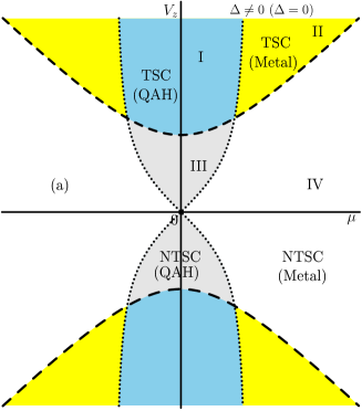
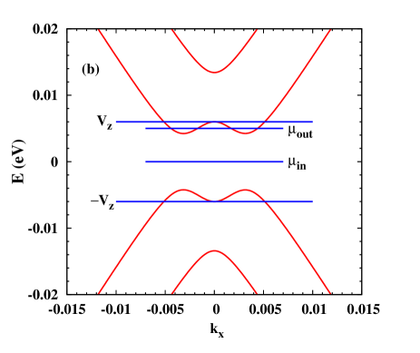
Figure 1: (Color online) (a) Topological phase diagram in the ($\mu,V_{z}$) space with $\Delta\neq 0$ or $\Delta=0$. The dashed curves, i.e., $V^{2}_{z}=\Delta^{2}+\mu^{2}$ are the phase boundaries between the TSC and NTSC whereas the dotted ones, i.e, $\mu^{2}=E_{0}^{2}$ stand for the phase boundaries between the QAH state and metal. (b) Bulk energy spectrum of $H_{e}^{\rm eff}$ near the $K$ point with $k_{y}=0$ and $\Delta=0$. $V_{z}$ ($-V_{z}$) is the upper (lower) limit of the chemical potential in the topological nontrivial regime ($V_{z}^{2}>\mu^{2}+\Delta^{2}$). $\mu_{\rm in}$ and $\mu_{\rm out}$ stand for the chemical potential in and out of the gap, respectively. $V_{z}=6\$meV and $\lambda=4\$meV.

Figure 2: (Color online) (a) and (b) represent the energy spectrum of zigzag graphene ribbon with the Rashba SOC, exchange field and proximity-induced $s$-wave superconductivity near the $K$ and $K^{\prime}$ points, respectively. (c) ((d)) Real space probability amplitude $|\psi|$ across the width for the Majorana edge state with a smaller (larger) $|k_{x}|$ near the $K$ point at one edge (i.e., $y=0$) with $v_{x}>0$ (only part of the ribbon is shown). A (B) refers to A (B) sublattice. The fluctuations of $|\psi|$ at the positions far away from the edge are due to numerical error. Here, $V_{z}=6\$meV, $\lambda=4\$meV, $\mu=0$ and $\Delta=2\$meV.

IV.2 Majorana edge states

As the effective $p$-wave superconductors (regime II) have been widely investigated in the literature,sau ; sau2 ; alicea2 ; lutchyn ; alicea3 ; halperin ; stanescu ; mourik ; yzhou ; bysun we concentrate on the TSC from the QAH state (regime I). The Majorana edge states are studied in thick graphene ribbons. The numerical method is detailed in Appendix C. We plot the energy spectrum of zigzag graphene ribbon near the $K$ and $K^{\prime}$ points in Figs. 2(a) and (b), respectively. We find that there exist four zero energy states in each valley. These eight states can be divided into two categories, i.e., four propagate along the same direction $+x$ ($-x$) determined by the group velocity $v_{x}=\frac{1}{\hbar}\frac{\partial E(k_{x})}{\partial k_{x}}$ $>0$ ($<0$). Moreover, the four states in the same category are at the same edge, which is in agreement with the magnitude of the Chern number, i.e., $|C_{1}|=4$. This indicates that these eight zero energy states are topologically protected Majorana edge states. Specifically, we choose two of them at the same edge with $v_{x}>0$ near the $K$ point and show the real space probability amplitude of the one with smaller and larger $|k_{x}|$ in Figs. 2(c) and (d), respectively. Note that we separate the A and B sublattices by the blue solid and red dashed curves. It is seen that the amplitudes of both A and B sublattices in two Majorana edge states show obvious decay and oscillation. However, the penetration lengths are different between these two Majorana edge states.

Figure 3: (Color online) Bulk excitation gap $E_{\rm gap}$ of the TSC from the QAH state as a function of $\Delta$. The solid curves with diamonds, crosses and plus signs correspond to the numerical results at $\mu=0$, $1\$meV and $2\$meV, respectively. The analytical results at $\mu=0$, $1\$meV and $2\$meV are separately represented by the symbols of squares, upward triangles and downward triangles. Note that for the analytical results at $\mu\neq 0$, only two limits, i.e., $\Delta\sim 0$ and $\Delta\sim\Delta_{c}$ are calculated. In addition, the dotted (dashed) curve corresponds to $E_{\rm gap}=\Delta$ ($E_{\rm gap}=10\Delta$). $V_{z}=6\$meV and $\lambda=4\$meV.

IV.3 Bulk excitation gap

IV.3.1 Chemical potential dependence

The above Majorana edge states are protected by a bulk excitation gap of the TSC from the QAH state. With different chemical potentials chosen in the gap of a QAH system, the bulk excitation gap as a function of the proximity-induced superconducting gap is plotted in Fig. 3. In the $\Delta=0$ limit, the system can be considered as two copies of QAH insulators as shown in Fig. 1(b) but with an energy shift of $-\mu$ ($\mu$) for the particle (hole) one. Then, the bulk excitation gap of our system is determined by these two QAH insulators, i.e., $E_{\rm gap}=E_{0}-|\mu|$. This nonzero bulk excitation gap in the limit $\Delta=0$ strongly indicates that the bulk excitation gap can be much larger than $\Delta$ especially for small $\Delta$. It is emphasized that the nonzero excitation gap in the $\Delta=0$ limit is totally different from the case of the effective $p$-wave superconductors where the excitation gap is exactly zero in the limit $\Delta=0$.alicea2 At the critical point $\Delta_{c}=\sqrt{V_{z}^{2}-\mu^{2}}$, the bulk excitation gap of our system becomes zero. In between, the bulk excitation gap shows a monotonic decrease with increasing $\Delta$. We emphasize that during this process, $E_{\rm gap}$ can be larger or even one order of magnitude larger than $\Delta$ by referring to $E_{\rm gap}=\Delta$ (dotted curve) and $E_{\rm gap}=10\Delta$ (dashed curve). For example, $E_{\rm gap}=4.02\$meV ($\Delta=0.3\$meV) at $\mu=0$; $E_{\rm gap}=3.22\$meV ($\Delta=0.3\$meV) at $\mu=1\$meV; $E_{\rm gap}=2.23\$meV ($\Delta=0.2\$meV) at $\mu=2\$meV. This marked enlargement of the gap is in strong contrast to the effective $p$-wave superconductors where the bulk excitation gap is always smaller than the induced superconducting gap.sau ; sau2 ; alicea2 ; lutchyn ; alicea3 ; halperin ; stanescu ; mourik ; yzhou ; bysun This makes our proposal, i.e., the TSC from the QAH state, very promising for the realization of robust Majorana modes in experiments.

To have a better understanding of the behavior of the bulk excitation gap of the TSC from the QAH state, we also perform an analytic derivation. Near the Dirac points, the BdG Hamiltonian $H_{\rm BdG}({\bf k})$ in Eq. (3) can be expanded as a low energy effective one with $H_{e}({\bf k})$ [see Eq. (10)] being replaced by $H^{\rm eff}_{e}({\bf k})$ [see Eq. (26)]. The secular equation of the eigenvalue $E$ is ${\rm det}[H_{\rm BdG}({\bf k})-EI_{8\times 8}]=0$ where $I_{8\times 8}$ is a unit matrix. After a careful calculation, we have

$$[\alpha_{1}^{2}-4V_{z}^{2}\alpha_{3}+4\alpha_{1}(\lambda_{R}^{2}-\mu^{2}-\mu V_{z})+4\alpha_{2}(\mu^{2}-\lambda_{R}^{2})]^{2}$$

$$\mbox{}-64V_{z}^{2}\alpha_{3}(\lambda_{R}^{2}-\mu^{2}-\mu V_{z})^{2}+8[\alpha_{1}\mu-2(\mu+V_{z})$$

$$\mbox{}\times(\mu^{2}-\lambda_{R}^{2})][(\mu+V_{z})(\alpha_{1}^{2}-4V_{z}^{2}\alpha_{3})-2\mu\alpha_{1}\alpha_{2}]=0$$

(20)

with $\alpha_{1}=\alpha_{2}-\alpha_{3}+\alpha_{4}$, $\alpha_{2}=v_{f}^{2}k_{x}^{2}$, $\alpha_{3}=E^{2}$, $\alpha_{4}=\Delta^{2}-V_{z}^{2}+\mu^{2}$, $v_{f}=3t/2$ and $\lambda_{R}=3\lambda/2$. Note that we focus on the calculation near the $K=(4\pi/3,0)$ ($\tau=1$) and set $k_{y}=0$ by considering the isotropy of the low energy effective Hamiltonian. It is very difficult to obtain the eigenvalues by solving Eq. (20) directly. Instead of the eigenvalues, we are interested in the bulk excitation gap here. Differentiating Eq. (20) with respect to $\alpha_{2}$ and then employing the extreme value condition of the excitation gap (i.e., $\frac{\partial\alpha_{3}}{\partial\alpha_{2}}=0$), we have

$$\alpha_{3}^{3}-g_{2}\alpha_{3}^{2}-g_{1}\alpha_{3}-g_{0}=0$$ (21)

where $g_{2}=3(\alpha_{2}+\alpha_{4})+2(2\lambda_{R}^{2}-\mu^{2}+2V_{z}^{2})$, $g_{1}=-3(\alpha_{2}+\alpha_{4})^{2}+4(-2\lambda_{R}^{2}-V_{z}^{2}+\mu^{2})(\alpha_{2}+\alpha_{4})+4\alpha_{2}(\lambda_{R}^{2}+\mu^{2})-8V_{z}^{2}(\lambda_{R}^{2}+\mu^{2})$ and $g_{0}=(\alpha_{2}+\alpha_{4})^{3}-2(\mu^{2}-2\lambda_{R}^{2})(\alpha_{2}+\alpha_{4})^{2}+4(\alpha_{2}+\alpha_{4})[\alpha_{2}(-\lambda_{R}^{2}-\mu^{2})-2\lambda_{R}^{2}(\mu^{2}-V_{z}^{2}-\lambda_{R}^{2})]+8\alpha_{2}(\mu^{4}-\lambda_{R}^{4})+8\alpha_{4}\lambda_{R}^{2}(\mu^{2}-\lambda_{R}^{2})$.

At $\mu=0$, Eq. (21) can be simplified to $(\alpha_{2}+\alpha_{4}-\alpha_{3})(4\alpha_{3}^{2}+q_{1}\alpha_{3}+q_{2})=0$ with $q_{1}=-8(\alpha_{2}+\alpha_{4})-16(\lambda_{R}^{2}+V_{z}^{2})$ and $q_{2}=4(\alpha_{2}+\alpha_{4})^{2}+16\lambda_{R}^{2}(\alpha_{2}+\alpha_{4})-16\lambda_{R}^{2}\alpha_{2}+32\lambda_{R}^{2}V_{z}^{2}$. Since the equation $4\alpha_{3}^{2}+q_{1}\alpha_{3}+q_{2}=0$ is inconsistent with the gap closing condition, we only have $\alpha_{2}+\alpha_{4}-\alpha_{3}=\alpha_{1}=0$. With this condition together with Eq. (20), one obtains the bulk excitation gap $E_{\rm gap}=E_{0}(1-|\Delta|/|V_{z}|)$, which is linearly dependent on $\Delta$ and agrees very well with the numerical results as shown in Fig. 3. Specially, for $E_{\rm gap}>|\Delta|$ ($E_{\rm gap}>10|\Delta|$), we have $|\Delta|<E_{0}|V_{z}|/(E_{0}+|V_{z}|)\equiv\Delta_{1}$ ($|\Delta|<E_{0}|V_{z}|/(E_{0}+10|V_{z}|)\equiv\Delta_{2}\approx 0.1E_{0}$). These conditions will guide the experiments to obtain robust TSCs and Majorana modes. As for the case of $\mu\neq 0$, it is very difficult for us to obtain an exact analytic solution. Only the analytical results in two limits, i.e., $|\Delta|\sim\Delta_{c}$ and $\Delta\sim 0$, are given. In the $|\Delta|\sim\Delta_{c}$ limit, we have $E_{\rm gap}=(\Delta_{c}-|\Delta|)\Delta^{2}_{c}|\mu^{2}-\lambda_{R}^{2}|/\sqrt{{V_{z}^{2}(\Delta_{c}^{2}+\lambda_{R}^{2})(\mu^{4}+\lambda_{R}^{2}\Delta_{c}^{2})}}$. In the limit $\Delta\sim 0$, $E_{\rm gap}=\sqrt{(E_{0}-\mu)^{2}-\Delta^{2}w_{2}/w_{1}}$ with $w_{1}=-\lambda_{R}^{2}\mu^{2}V_{z}^{2}+\mu(\lambda_{R}^{2}+V_{z}^{2})(-\lambda_{R}^{2}+\mu^{2}-V_{z}^{2})E_{0}$ and $w_{2}=\mu(\lambda_{R}^{2}-\mu^{2})(\lambda_{R}^{2}+V_{z}^{2})E_{0}-16\lambda_{R}^{2}V_{z}^{2}(\lambda_{R}^{4}-\mu^{2}V_{z}^{2}-2\lambda_{R}^{2}\mu^{2}+\lambda_{R}^{2}V_{z}^{2})/(\lambda_{R}^{2}+V_{z}^{2})$ by assuming $0<\mu<E_{0}$. The analytical results at $\mu\neq 0$ in both limits agree fairly well with the numerical ones as shown in Fig. 3.

Figure 4: (Color online) Numerical results of bulk excitation gap $E_{\rm gap}$ of the TSC from the QAH state as a function of the proximity-induced superconducting gap $\Delta$ at $\mu=0$ (a) under different $\lambda$ with $V_{z}=6\$meV and (b) under different $V_{z}$ with $\lambda=4\$meV.

IV.3.2 Rashba SOC strength and exchange field dependences

We then turn to investigate the effects of the Rashba SOC and exchange field on the bulk excitation gap of the TSC from the QAH state. In Figs. 4(a) and (b), we plot the dependence of the bulk excitation gap on the proximity-induced superconducting gap at $\mu=0$ under different Rashba SOC strengths and exchange fields, respectively. It is seen that the bulk excitation gap increases with the increase of either the Rashba SOC strength or exchange field. This can be easily understood from $E_{\rm gap}=E_{0}(1-|\Delta|/|V_{z}|)$ mentioned above where $E_{0}$ (see Appendix A) increases with increasing Rashba SOC strength and exchange field.

V SUMMARY AND DISCUSSION

In summary, we have proposed that in the presence of proximity-induced $s$-wave superconductivity, the QAH state due to the Rashba SOC and exchange field in single layer graphene can become a two-dimensional TSC. With very low or even zero doping near the Dirac points, i.e., two inequivalent valleys, we show that this TSC, which exhibits a Chern number as large as four and hosts four Majorana edge modes, has a bulk excitation gap being larger or even one order of magnitude lager than the proximity-induced superconducting gap. The unique feature is in strong contrast to the case of the effective $p$-wave superconductors where the bulk excitation gap is always smaller than the proximity-induced superconducting gap. This also applies to other QAH systems as seed materials to obtain robust TSCs and Majorana modes.

Finally, we address the experimental feasibility of the TSC from the QAH state. Single layer graphene on the (111) surface of an antiferromagnetic insulator BiFeO₃ can have an exchange field ($V_{z}=142\$meV) and Rashba SOC ($\lambda=1.4\$meV), realizing a QAH insulator with a gap being $2E_{0}=4.2\$meV.qiao2 This QAH state ($|\mu|<E_{0}$) in proximity to a conventional $s$-wave superconductor (eg., Nb with a large superconducting gap $\Delta_{\rm Nb}=0.83\$meV jwang ) becomes a TSC since the topologically nontrivial condition $\Delta^{2}+\mu^{2}<V_{z}^{2}$ is easily satisfied due to $|\mu|<E_{0}\ll|V_{z}|$ and $|\Delta|<|\Delta_{\rm Nb}|\ll|V_{z}|$. With $\Delta=0.5\$meV ($\Delta_{2}=0.21\$meV $<\Delta<\Delta_{1}=2.1\$meV) for estimation, we have the bulk excitation gap $E_{\rm gap}=2.05\$meV, $1.56\$meV and $1.06\$meV, corresponding to a temperature of $23.8\$K, $18.1\$K and $12.3\$K, at $\mu=0$, $0.5\$meV and $1\$meV, respectively. The large excitation gap (of the order of $10\$K) ensures that robust Majorana modes can be achieved.

Appendix A $H_{e}({\bf k})$ in Eq. (3) near the Dirac points

Near the Dirac points, i.e., $K=(4\pi/3,0)\ (\tau=1)$ and $K^{\prime}=(-4\pi/3,0)\ (\tau=-1)$, $H_{e}({\bf k})$ in Eq. (3) can be expanded as a low energy effective Hamiltonian

$$H^{\rm eff}_{e}({\bf k})=\left(\begin{array}[]{cccc}V_{z}&v_{f}(\tau k_{x}-ik_{y})&0&i\lambda_{R}(1-\tau)\\ v_{f}(\tau k_{x}+ik_{y})&V_{z}&-i\lambda_{R}(1+\tau)&0\\ 0&i\lambda_{R}(1+\tau)&-V_{z}&v_{f}(\tau k_{x}-ik_{y})\\ i\lambda_{R}(\tau-1)&0&v_{f}(\tau k_{x}+ik_{y})&-V_{z}\end{array}\right).$$ (26)

The energy spectrum of this effective Hamiltonian is shown in Fig. 1(b). The minimum (maximum) energy of the conduction (valence) band is $E_{0}=|V_{z}\lambda_{R}|/\sqrt{V_{z}^{2}+\lambda_{R}^{2}}$ ($-E_{0}$) after a simple calculation and then the band gap is given by $2E_{0}$.

Appendix B Gap closing condition of the BdG Hamiltonian $H_{\rm BdG}({\bf k})$

The gap of $H_{\rm BdG}({\bf k})$ closes at the momenta $\Gamma$ (single one), $M$ (three inequivalent ones) and $K$ (two inequivalent ones) points. Specifically, at the momentum $\Gamma$, the Rashba SOC vanishes [see Eq. (10)], which is similar to the previous studies in semiconductors.sau ; sau2 The gap closing condition is given by $(\mu\pm 3t)^{2}=V^{2}_{z}-\Delta^{2}$ with $+$ ($-$) representing lower (higher) energy band at $\Gamma$ after a simple calculation. As for the momentum $M$, the Rashba SOC does not cause spin splitting but lead to an energy shift for the spin degenerate bands. We take $M=(0,\frac{2\sqrt{3}\pi}{3})$ for example and $H_{\rm BdG}(M)$ [see Eq. (3)] reads

$$H_{\rm BdG}(M)=\left(\begin{array}[]{cccccccc}-\mu+V_{z}&\frac{\sqrt{3}i-1}{2}t&0&-\lambda(i+\sqrt{3})&\Delta&0&0&0\\ \frac{-\sqrt{3}i-1}{2}t&-\mu+V_{z}&-\lambda(\sqrt{3}-i)&0&0&\Delta&0&0\\ 0&-\lambda(i+\sqrt{3})&-\mu-V_{z}&\frac{\sqrt{3}i-1}{2}t&0&0&\Delta&0\\ -\lambda(\sqrt{3}-i)&0&\frac{-\sqrt{3}i-1}{2}t&-\mu-V_{z}&0&0&0&\Delta\\ \Delta&0&0&0&\mu+V_{z}&-\frac{\sqrt{3}i-1}{2}t&0&\lambda(i+\sqrt{3})\\ 0&\Delta&0&0&\frac{\sqrt{3}i+1}{2}t&\mu+V_{z}&\lambda(\sqrt{3}-i)&0\\ 0&0&\Delta&0&0&\lambda(i+\sqrt{3})&\mu-V_{z}&-\frac{\sqrt{3}i-1}{2}t\\ 0&0&0&\Delta&\lambda(\sqrt{3}-i)&0&\frac{\sqrt{3}i+1}{2}t&\mu-V_{z}\end{array}\right).$$ (35)

Performing a unitary transformation as $\tilde{H}_{\rm BdG}(M)=U_{M}^{\dagger}H_{\rm BdG}(M)U_{M}$ with

$$U_{M}=\frac{\sqrt{2}}{2}\left(\begin{array}[]{cccccccc}0&\frac{1-\sqrt{3}i}{2}&0&\frac{-1+\sqrt{3}i}{2}&0&0&0&0\\ 0&1&0&1&0&0&0&0\\ \frac{1-\sqrt{3}i}{2}&0&\frac{-1+\sqrt{3}i}{2}&0&0&0&0&0\\ 1&0&1&0&0&0&0&0\\ 0&0&0&0&0&\frac{1-\sqrt{3}i}{2}&0&\frac{-1+\sqrt{3}i}{2}\\ 0&0&0&0&0&1&0&1\\ 0&0&0&0&\frac{1-\sqrt{3}i}{2}&0&\frac{-1+\sqrt{3}i}{2}&0\\ 0&0&0&0&1&0&1&0\end{array}\right),$$ (44)

one obtains

$$\tilde{H}_{\rm BdG}(M)=\left(\begin{array}[]{cccccccc}-t-\mu-V_{z}&0&0&-2i\lambda&\Delta&0&0&0\\ 0&-t-\mu+V_{z}&-2i\lambda&0&0&\Delta&0&0\\ 0&2i\lambda&t-\mu-V_{z}&0&0&0&\Delta&0\\ 2i\lambda&0&0&t-\mu+V_{z}&0&0&0&\Delta\\ \Delta&0&0&0&t+\mu-V_{z}&0&0&2i\lambda\\ 0&\Delta&0&0&0&t+\mu+V_{z}&2i\lambda&0\\ 0&0&\Delta&0&0&-2i\lambda&-t+\mu-V_{z}&0\\ 0&0&0&\Delta&-2i\lambda&0&0&-t+\mu+V_{z}\end{array}\right).$$ (53)

At $\mu\sim t$, the block with the diagonal terms being $-t-\mu\mp V_{z}$ and $t+\mu\mp V_{z}$ in $\tilde{H}_{\rm BdG}(M)$ is far from gap closing whereas the gap closing is determined by the remaining one. By considering that $|\lambda|\ll t$, we use the Löwdin partition method lowdin ; winkler to obtain the effective Hamiltonian for the block determining the gap closing as

$$H_{\rm eff}(M)=\left(\begin{array}[]{cccc}t-\mu-V_{z}+\frac{2\lambda^{2}}{t-V_{z}}&0&\Delta&0\\ 0&t-\mu+V_{z}+\frac{2\lambda^{2}}{t+V_{z}}&0&\Delta\\ \Delta&0&-t+\mu-V_{z}-\frac{2\lambda^{2}}{t+V_{z}}&0\\ 0&\Delta&0&-t+\mu+V_{z}+\frac{2\lambda^{2}}{-t+V_{z}}\end{array}\right).$$ (58)

Then, the gap closing condition is $(t-\mu-V_{z}+\frac{2\lambda^{2}}{t-V_{z}})(-t+\mu-V_{z}-\frac{2\lambda^{2}}{t+V_{z}})-\Delta^{2}=0$ or $(t-\mu+V_{z}+\frac{2\lambda^{2}}{t+V_{z}})(-t+\mu+V_{z}-\frac{2\lambda^{2}}{-t+V_{z}})-\Delta^{2}=0$. As $|V_{z}|\ll t$, both conditions become $(t-\mu+\frac{2\lambda^{2}}{t})^{2}=V_{z}^{2}-\Delta^{2}$ approximately. Furthermore, by considering that $|\lambda|\ll t$, we neglect the energy shift of $2\lambda^{2}/{t}$ and then the gap closing condition at the momentum $M$ with $\mu\sim t$ is given by $(t-\mu)^{2}=V_{z}^{2}-\Delta^{2}$. Similarly, the gap closing condition at $M$ with $\mu\sim-t$ is $(t+\mu)^{2}=V_{z}^{2}-\Delta^{2}$ under the approximation $|\lambda|,|V_{z}|\ll t$.

In contrast to the momenta $\Gamma$ and $M$, the Rashba SOC at the Dirac points contributes to a finite spin splitting. Specifically, with $K=(4\pi/3,0)$, $H_{\rm BdG}(K)$ [see Eq. (3)] can be written as

$$H_{\rm BdG}({K})=\left(\begin{array}[]{cccccccc}-\mu+V_{z}&0&0&0&\Delta&0&0&0\\ 0&-\mu+V_{z}&-3i\lambda&0&0&\Delta&0&0\\ 0&3i\lambda&-\mu-V_{z}&0&0&0&\Delta&0\\ 0&0&0&-\mu-V_{z}&0&0&0&\Delta\\ \Delta&0&0&0&\mu+V_{z}&0&0&0\\ 0&\Delta&0&0&0&\mu+V_{z}&3i\lambda&0\\ 0&0&\Delta&0&0&-3i\lambda&\mu-V_{z}&0\\ 0&0&0&\Delta&0&0&0&\mu-V_{z}\\ \end{array}\right),$$ (67)

which can be divided into two independent $4\times 4$ parts, i.e., $H_{1}$ ($H_{2}$) without (with) the Rashba SOC terms. Then, we have

$$H_{1}=\left(\begin{array}[]{cccc}-\mu+V_{z}&0&\Delta&0\\ 0&-\mu-V_{z}&0&\Delta\\ \Delta&0&\mu+V_{z}&0\\ 0&\Delta&0&\mu-V_{z}\\ \end{array}\right),$$ (72)

which is exactly the same as the Hamiltonian of semiconductors with the Rashba SOC, magnetic field and proximity-induced $s$-wave superconductivity at the momentum $\Gamma$.sau ; sau2 This indicates that both have the same gap closing condition, i.e., $V^{2}_{z}=\mu^{2}+\Delta^{2}$.sau ; sau2 As for $H_{2}$ (not shown), due to the existence of the nonzero Rashba SOC terms, the gap is always opened. Therefore, the gap closing condition at $K$ is just the one in $H_{1}$ part. Similar analysis can be applied to $K^{\prime}$ and we obtain the same gap closing condition as $K$.

Appendix C Numerical method for calculating Majorana edge states in zigzag and armchair graphene ribbons

We investigate the Majorana edge states near the Dirac points in both zigzag and armchair graphene ribbons. We first study the case of zigzag configuration. The Hamiltonian of zigzag ribbon can be obtained from Eq. (1) by choosing a unit cell and performing a Fourier transformation along the direction parallel to the edge (assuming $x$-direction). Note that the unit cell of the zigzag ribbon is the same as the one in Ref. brey, . Specifically,

$$H_{\rm zigzag} = -t\sum_{k_{x}}\sum_{\langle j_{1},j_{2}\rangle\sigma}[1+|{\rm sgn}(x_{j_{2}}-x_{j_{1}})|e^{ik_{x}{\rm sgn}(x_{j_{2}}-x_{j_{1}})}]c^{\dagger}_{k_{x}j_{1}\sigma}c_{k_{x}j_{2}\sigma}+\sum_{k_{x}}\sum_{j\sigma}(\sigma V_{z}-\mu)c^{\dagger}_{k_{x}j\sigma}c_{k_{x}j\sigma}$$ (73)

$$\mbox{}+\Delta\sum_{k_{x}}\sum_{j}(c^{\dagger}_{k_{x}j\uparrow}c^{\dagger}_{-k_{x}j\downarrow}+{\rm H.c.})+i\lambda\sum_{k_{x}}\sum_{\langle j_{1},j_{2}\rangle\sigma\sigma^{\prime}}[(\sigma_{x}^{\sigma\sigma^{\prime}}d^{y}_{j_{1}j_{2}}-\sigma_{y}^{\sigma\sigma^{\prime}}d^{x}_{j_{1}j_{2}})+|{\rm sgn}(x_{j_{2}}-x_{j_{1}})|e^{ik_{x}{\rm sgn}(x_{j_{2}}-x_{j_{1}})}$$

$$\mbox{}\times(\sigma_{x}^{\sigma\sigma^{\prime}}d^{y}_{j_{1}j_{2}}+\sigma_{y}^{\sigma\sigma^{\prime}}d^{x}_{j_{1}j_{2}})]c^{\dagger}_{k_{x}j_{1}\sigma}c_{k_{x}j_{2}\sigma^{\prime}}$$

where $x_{j_{2}}-x_{j_{1}}$ is the relative position between $j_{2}$-th and $j_{1}$-th atoms in the unit cell along the $x$-direction and sgn stands for the sign function. By exactly diagonalizing $H_{\rm zigzag}$, one obtains the eigenvalues and eigenstates. However, this method fails due to the computational limitations when the width of the ribbon becomes very large (eg., of the order of $10^{4}$ atoms in the unit cell in our calculation). Alternatively, the zigzag ribbon with the leading term, i.e., the hopping term, can be solved analytically near the Dirac points.neto Near $K$ ($\tau=1$) and $K^{\prime}$ ($\tau=-1$), the eigenstates are given by

$$\Psi_{\tau k_{x}}^{z,\varepsilon}({\bf r}) = Ae^{i(\tau|K|+k_{x})x}$$ (76)

$$\mbox{}\times\left(\begin{array}[]{c}-v_{f}[(z-\tau k_{x})e^{zy}+(z+\tau k_{x})e^{-zy}]/\varepsilon\\ e^{zy}-e^{-zy}\\ \end{array}\right),$$

with the eigenvalues being $\varepsilon^{2}=v_{f}^{2}(k_{x}^{2}-z^{2})$ and $A=\sqrt{\frac{\sqrt{3}}{|2(e^{2zL}-e^{-2zL})/z-8L|}}$. $L$ is the width of the ribbon and $z$ is determined by the equation $e^{-2zL}=(k_{x}+\tau z)/(k_{x}-\tau z)$. Note that if $z_{0}$ is a solution of this equation, so does $-z_{0}$. As $\Psi_{\tau k_{x}}^{z_{0},\varepsilon}=-\Psi_{\tau k_{x}}^{-z_{0},\varepsilon}$, only one of these two equivalent eigenstates needs to be taken. Then, one can use these eigenstates in Eq. (76) with additional spin and particle-hole degrees of freedom included to construct complete basis functions for $H_{\rm zigzag}$. We diagonalize the Hamiltonian matrix of $H_{\rm zigzag}$ and obtain the energy spectrum and wavefunctions as shown in Fig. 2.

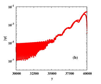
Figure 5: (Color online) (a) Energy spectrum of armchair graphene ribbon in the presence of the Rashba SOC, exchange field and $s$-wave superconductivity from the proximity effect. (b) ((c)) Real space probability amplitude $|\psi|$ across the width for the Majorana edge state with a smaller (larger) momentum $|k_{x}|$ ($k_{x}<0$) at one edge (i.e., $y=40000$) (only part of the ribbon is shown). The fluctuations of $|\psi|$ at the positions far away from the edge are due to numerical error. Here, $V_{z}=6\$meV, $\lambda=4\$meV, $\mu=2\$meV and $\Delta=2\$meV.

We turn to the case of armchair graphene ribbon with the Hamiltonian being

$$H_{\rm armchair} = -t\sum_{k_{x}}\sum_{\langle j_{1},j_{2}\rangle\sigma}c^{\dagger}_{k_{x}j_{1}\sigma}c_{k_{x}j_{2}\sigma}+\sum_{k_{x}}\sum_{j\sigma}(\sigma V_{z}-\mu)c^{\dagger}_{k_{x}j\sigma}c_{k_{x}j\sigma}+\Delta\sum_{k_{x}}\sum_{j}(c^{\dagger}_{k_{x}j\uparrow}c^{\dagger}_{-k_{x}j\downarrow}+{\rm H.c.})$$ (77)

$$\mbox{}+i\lambda\sum_{k_{x}}\sum_{\langle j_{1},j_{2}\rangle\sigma\sigma^{\prime}}(\sigma_{x}^{\sigma\sigma^{\prime}}d^{y}_{j_{1}j_{2}}-\sigma_{y}^{\sigma\sigma^{\prime}}d^{x}_{j_{1}j_{2}})c^{\dagger}_{k_{x}j_{1}\sigma}c_{k_{x}j_{2}\sigma^{\prime}}-t\sum_{k_{x}}\sum_{j^{*}_{1}j^{*}_{2}\sigma}[e^{i\sqrt{3}k_{x}}(\delta_{j^{*}_{1},j^{*}_{2}}+\delta_{j^{*}_{1}+1,j^{*}_{2}})c^{\dagger}_{k_{x}j^{*}_{1}\sigma}c_{k_{x}j^{*}_{2}\sigma}+{\rm H.c.}]$$

$$\mbox{}+i\lambda\sum_{k_{x}}\sum_{j^{*}_{1}j^{*}_{2}\sigma\sigma^{\prime}}\{e^{i\sqrt{3}k_{x}}[\delta_{j^{*}_{1}+1,j^{*}_{2}}(\frac{\sqrt{3}}{2}\sigma_{x}^{\sigma\sigma^{\prime}}-\frac{1}{2}\sigma_{y}^{\sigma\sigma^{\prime}})-\delta_{j^{*}_{1},j^{*}_{2}}(\frac{\sqrt{3}}{2}\sigma_{x}^{\sigma\sigma^{\prime}}+\frac{1}{2}\sigma_{y}^{\sigma\sigma^{\prime}})]c^{\dagger}_{k_{x}j^{*}_{1}\sigma}c_{k_{x}j^{*}_{2}\sigma^{\prime}}+{\rm H.c.}\}$$

in which $j^{*}_{1}$ ($j^{*}_{2}$) represents the $j^{*}_{1}$-th ($j^{*}_{2}$-th) atom of the first (fourth) column in the unit cell. Note that the unit cell of the armchair ribbon is the same as the one in Ref. brey, and the edges lie along the $x$-direction. Similar to the case of the zigzag graphene ribbon, we first solve the armchair ribbon with only the hopping term analytically near the Dirac points. The eigenstates read

$$\Psi_{k_{x}}^{k_{n},\varepsilon}({\bf r}) = 2Ae^{ik_{x}x}\sin[(|K|+k_{n})y]$$ (80)

$$\mbox{}\times\left(\begin{array}[]{c}-v_{f}(k_{x}-ik_{n})/\varepsilon\\ i\\ \end{array}\right),$$

where the eigenvalues are $\varepsilon^{2}=v_{f}^{2}(k_{x}^{2}+k_{n}^{2})$ with $k_{n}=n\pi/L-|K|$ and $A=\frac{1}{\sqrt{8L}}$. These eigenstates construct complete basis functions for $H_{\rm armchair}$ with additional spin and particle-hole degrees of freedom. By diagonalizing the Hamiltonian matrix, one obtains the energy spectrum and eigenstates of armchair graphene ribbon as shown in Fig. 5. In Fig. 5(a), we find that there exist eight zero energy states, corresponding to four Majorana fermions at each edge, which is similar to the case of zigzag ribbon. We then show the real space probability amplitude of two Majorana edge states at the same edge with a smaller and larger momentum $|k_{x}|$ ($k_{x}<0$) in Figs. 5(b) and (c), respectively. It is seen that both show obvious decays and oscillations but the decay lengths and oscillation periods are different.

References

• (1) A. Y. Kitaev, Phys. Usp. 44, 131 (2001).
• (2) J. Alicea, Rep. Prog. Phys. 75, 076501 (2012).
• (3) C. W. Beenakker, Annu. Rev. Condens. Matter Phys. 4, 113 (2013).
• (4) M. Z. Hasan and C. L. Kane, Rev. Mod. Phys. 82, 3045 (2010).
• (5) X.-L. Qi and S.-C. Zhang, Rev. Mod. Phys. 83, 1057 (2011).
• (6) D. A. Ivanov, Phys. Rev. Lett. 86, 268 (2001).
• (7) A. P. Mackenzie and Y. Maeno, Rev. Mod. Phys. 75, 657 (2003).
• (8) L. Fu and C. L. Kane, Phys. Rev. Lett. 100, 096407 (2008).
• (9) J. D. Sau, R. M. Lutchyn, S. Tewari, and S. Das Sarma, Phys. Rev. Lett. 104, 040502 (2010).
• (10) J. D. Sau, S. Tewari, R. M. Lutchyn, T. D. Dtanescu, and S. Das Sarma, Phys. Rev. B 82, 214509 (2010).
• (11) J. Alicea, Phys. Rev. B 81, 125318 (2010).
• (12) R. M. Lutchyn, J. D. Sau, and S. Das Sarma, Phys. Rev. Lett. 105, 077001 (2010).
• (13) J. Alicea, Y. Oreg, G. Refael, F. von Oppen, and M. P. A. Fisher, Nature Phys. 7, 412 (2011).
• (14) B. I. Halperin, Y. Oreg, A. Stern, G. Refael, J. Alicea, and F. von Oppen, Phys. Rev. B 85, 144501 (2012).
• (15) T. D. Stanescu and S. Tewari, J. Phys.: Condens. Matter 25, 233201 (2013).
• (16) V. Mourik, K. Zuo, S. M. Frolov, S. R. Plissard, E. P. A. M. Bakkers, and L. P. Kouwenhoven, Science 336, 1003 (2012).
• (17) Y. Zhou and M. W. Wu, J. Phys.: Condens. Matter 26, 065801 (2014).
• (18) B. Y. Sun and M. W. Wu, New J. Phys. 16, 073045 (2014).
• (19) J. J. He, J. Wu, T.-P. Choy, X.-J. Liu, Y. Tanaka, and K. T. Law, Nat. Commmun. 5, 3232 (2014).
• (20) S. Tewari and J. D. Sau, Phys. Rev. Lett. 109, 150408 (2012).
• (21) S. Tewari, T. D. Stanescu, J. D. Sau, and S. Das Sarma, Phys. Rev. B 86, 024504 (2012).
• (22) M. Diez, J. P. Dahlhaus, M. Wimmer, and C. W. J. Beenakker, Phys. Rev. B 86, 094501 (2012).
• (23) C. L. M. Wong, J. Liu, K. T. Law, and P. A. Lee, Phys. Rev. B 88, 060504(R) (2013).
• (24) A. Haim, A. Keselman, E. Berg, and Y. Oreg, Phys. Rev. B 89, 220504(R) (2014).
• (25) C. Dutreix, M. Guigou, D. Chevallier, and C. Bena, Eur. Phys. J. B 87, 296 (2014).
• (26) S. Nadj-Perge, I. K. Drozdov, J. Li, H. Chen, S. Jeon, J. Seo, A. H. MacDonld, B. A. Bernevig, and A. Yazdani, Science 346, 602 (2014).
• (27) J. Li, H. Chen, I. K. Drozdov, A. Yazdani, B. A. Bernevig, and A. H. MacDonald, Phys. Rev. B 90, 235433 (2014).
• (28) H.-Y. Hui, P. M. R. Brydon, J. D. Sau, S. Tewari, and S. Das Sarma, Sci. Rep. 5, 8880 (2015).
• (29) E. Dumitrescu, B. Roberts, S. Tewari, J. D. Sau, and S. Das Sarma, Phys. Rev. B 91, 094505 (2015).
• (30) K. Pöyhönen, A. Westström, and T. Ojanen, arXiv:1509.05223.
• (31) J. Röntynen and T. Ojanen, Phys. Rev. Lett. 114, 236803 (2015).
• (32) J. Li, T. Neupert, Z. J. Wang, A. H. MacDonald, A. Yazdani, and B. Andrei Bernevig, arXiv:1501.00999.
• (33) X.-L. Qi, T. L. Hughes, and S.-C. Zhang, Phys. Rev. B 82, 184516 (2010).
• (34) J. Wang, Q. Zhou, B. Lian, and S.-C. Zhang, Phys. Rev. B 92, 064520 (2015).
• (35) A. P. Schnyder, S. Ryu, A. Furusaki, and A. W. W. Ludwig, Phys. Rev. B 78, 195125 (2008).
• (36) Z. Qiao, S. A. Yang, W. Feng, W.-K. Tse, J. Ding, Y. Yao, J. Wang, and Q. Niu, Phys. Rev. B 82, 161414(R) (2010).
• (37) Y. A. Bychkov and E. I. Rashba, J. Phys. C 17, 6039 (1984); Pis’ma Zh. Eksp. Teor. Fiz. 39, 66 (1984) [JETP Lett. 39, 78 (1984)].
• (38) C. Niu, P. M. Buhl, G. Bihlmayer, D. Wortmann, S. Blügel, and Y. Mokrousov, Phys. Rev. B 91, 201401(R) (2015).
• (39) Z. H. Qiao, W. Ren, H. Chen, L. Bellaiche, Z. Y. Zhang, A. H. MacDonald, and Q. Niu, Phys. Rev. Lett. 112, 116404 (2014).
• (40) G. Xu, B. Lian, and S.-C. Zhang, Phys. Rev. Lett. 115, 186802 (2015).
• (41) C. L. Kane and E. J. Mele, Phys. Rev. Lett. 95, 146802 (2005).
• (42) M. Ezawa, Y. Tanaka, and N. Nagaosa, Sci. Rep. 3, 2790 (2013).
• (43) A. H. Castro Neto, F. Guinea, N. M. R. Peres, K. S. Novoselov, and A. K. Geim, Rev. Mod. Phys. 81, 109 (2009).
• (44) P. Ghosh, J. D. Sau, S. Tewari, and S. Das Sarma, Phys. Rev. B 82, 184525 (2010).
• (45) P. O. Löwdin, J. Chem. Phys. 19, 1396 (1951).
• (46) R. Winkler, Spin-Orbit Coupling Effects in Two-Dimensional Electron and Hole Systems (Springer, Berlin, 2003).
• (47) L. Brey and H. A. Fertig, Phys. Rev. B 73, 235411 (2006).