Current helicity and magnetic field anisotropy in solar active regions

Abstract

The electric current helicity density $\displaystyle\chi=\langle\epsilon_{ijk}b_{i}\frac{\partial b_{k}}{\partial x_{j}}\rangle$ contains six terms, where $b_{i}$ are components of the magnetic field. Due to the observational limitations, only four of the above six terms can be inferred from solar photospheric vector magnetograms. By comparing the results for simulation we distinguished the statistical difference of above six terms for isotropic and anisotropic cases. We estimated the relative degree of anisotropy for three typical active regions and found that it is of order 0.8 which means the assumption of local isotropy for the observable current helicity density terms is generally not satisfied for solar active regions. Upon studies of the statistical properties of the anisotropy of magnetic field of solar active regions with latitudes and with evolution in the solar cycle, we conclude that the consistency of that assumption of local homogeneity and isotropy requires further analysis in the light of our findings.

1 Introduction

Solar magnetic cycle is believed to be excited by solar dynamo mechanism based on a joint action of differential rotation and mirror-asymmetric convection. Differential rotation known from helioseismology produces toroidal large-scale magnetic field from poloidal one while mirror asymmetric convection is responsible for transformation of the toroidal large-scale magnetic field into poloidal one in order to close the chain of self-excitation. Simple symmetry arguments show that a link between the toroidal and poloidal magnetic fields must be governed by a mirror-asymmetric quantity (generally a pseudo tensor) , however, there are several ways on how to implement this link in particulars (e.g. by notion of cyclonic motions, Parker (1955); or by magnetic tubes arising and being twisted by Coriolis force, as in Babcock (1961), Leighton (1969) mechanism, what gives a variety of solar dynamo models. From the other hand, the degree of mirror asymmetry is believed to be moderate and the very degree of mirror asymmetry seems to be hardly determined from observational data. The point is that in order to quantify the mirror asymmetry of a dynamo one has to know 3D distribution of the mean-field characteristics and compute their spatial derivatives.

For example, a more straightforward quantity known as hydrodynamic (or kinetic) helicity density $\langle{\bf v}\cdot{\rm curl\,}{\bf v}\rangle$ which determines the excess of right-hand helixes against left-hand ones requires 3D distribution of velocity field $\bf v$ and its derivatives while conventional Doppler-effect gives line-of-sight velocities only. Note that we are interested in averaging quantities and $\langle\dots\rangle$ means corresponding averaging. While in mean-field dynamo theory the averaging is carried out over the ensembles of turbulent pulsations, practically given the observational data in vector magnetograms of solar active regions, we average by area in the available field-of-view of something similar to that.

A practically accessible way to quantify mirror asymmetry observationally was firstly suggested by Seehafer (1990). He pointed out that vector magnetographic observations provide three magnetic field components on a surface $z={\rm const}$ at solar atmosphere (local coordinates $x$ and $y$ are parallel to the solar surface, and for a limited field of view we can ignore the effect of curvature). He used the force-free field parameter $\alpha$ as a proxy of electric current helicity. The available vector magnetic field is not sufficient to calculate the entire current helicity density $\chi=\langle{\bf B}\cdot{\rm curl\,}{\bf B}\rangle$ and to quantify relative number of right handed twisted magnetic tubes against left-handed ones, however, one can calculate a mirror-asymmetric quantity

$$\chi_{z}=\langle B_{z}({\rm curl\,}{\bf B})_{z}\rangle=\left\langle B_{z}\left({{\triangledown_{x}B_{y}}}-{{\triangledown_{y}B_{x}}}\right)\right\rangle\,,$$ (1)

which makes one of the three believed to be similar contributions to the entire quantity $\chi$, i.e., $\chi_{x}$ and $\chi_{y}$ (they can be obtained from Eq. (1) by circular replacement of indices). Note that $\chi_{z}$ do not contain derivative in direction $z$. If magnetic field $\bf B$ is locally statistically isotropic, all three contribution in $\chi$ are statistically equal and the natural consequence is

$$\chi=3\chi_{z}\,.$$ (2)

The force-free field parameter $\alpha$ and the current helicity parameter $\chi$ become available for observational determination in solar active regions (see, e.g., Pevtsov, 1994; Abramenko et al., 1996; Bao & Zhang, 1998; Hagino and Sakurai, 2004). The above statistical studies show that the sign of $\alpha$ and $\chi$ is same, which is predominantly negative in the northern hemisphere and positive in the southern hemisphere. Results of monitoring $\chi_{z}$ in two last solar cycles and butterfly diagrams for solar cyclic variation of this quantity are presented in Zhang et al. (2010). The quantity followed the helicity polarity rule as well as pronounced areas on the butterfly diagrams where the polarity rule is inverted (Zhang et al., 2010). The result looks instructive for solar dynamo modeling (Zhang et al., 2012). Dynamo interpretation of the observational data is usually based on assumption of the local statistical isotropy, and so $\chi_{z}$ is considered as an observational tracer for $\chi$.

Conventional theory of turbulence is originated from Kolmogorov (1941), while Iroshnikov (1963) and Kraichnan (1965) ideas presumes that the velocity and magnetic fields become statistically homogeneous in sufficiently small scales (though Goldreich and Sridhar (1997) have stressed the role of magnetic field anisotropy in MHD turbulence). It is however not clear what scales in the solar photospheres can be considered as homogeneous enough for this assumption and whether typical active regions may fall under this consideration. A perspective to verify to what extent the solar magnetic field at the scale of active regions can be considered as statistically isotropic has not been yet considered observationally at least in the approach suggested by Seehafer (1990): the point is that calculation of other contributions to the current helicity to be compared with $\chi_{z}$ would require derivatives of magnetic field components in $z$ direction while in fact we have three components of the magnetic field at surface $z={\rm const}$ only.

The aim of this paper is to show that one can refurnish the approach of Seehafer (1990) in a way to verify the hypothesis of local isotropy in the scales of active regions. Instead of to present $\chi$ as a sum of three contributions $\chi_{z}$, $\chi_{x}$ and $\chi_{y}$ which have to be equal in a locally isotropic case, we present this quantity as a sum of six quantities to be equal in the isotropic case. Four out of the six quantities do not contain derivatives in $z$ direction and are potentially accessible for observations.

We demonstrate that the available bulk of data for the magnetic field vector in solar active regions enable us to obtain statistically robust estimates for the four quantities. Local statistical isotropy implies two pairs of identities for the above four quantities. We show that one pair of the identities holds while the other fails being confronted with the observational data. We may believe that the magnetic field occurs to be substantially statistically anisotropic in scales of active regions. As a result, the quantity $\chi_{z}$ which has been traced for last two solar cycles has to be considered as a specific mirror asymmetric tracer of anisotropic solar MHD rather than purely $\chi/3$. We discuss the importance of this conclusion for solar dynamo models.

2 Observational Data

We used 6629 vector magnetograms observed by Solar Magnetic Field Telescope (SMFT) at Huairou Solar Observing Station from 1988 to 2005. This data sample was used earlier by Gao et al. (2008) and Zhang et al. (2010). The SMFT is equipped with a birefringent filter for wavelength selection and KD*P crystals to modulate polarization signals. The Fe 1 5324.19 Å line is used. A vector magnetogram is built using four narrow-band (0.125Å) filtergrams of Stokes I, Q, U and V parameters. The center wavelength of the filter can be shifted and is normally at -0.075 Å for the measurements of longitudinal magnetic field and at the line center for the transversal magnetic fields (Ai & Hu, 1986). The $180^{\circ}$ ambiguity in the azimuth angle ($\phi$) was resolved following Wang, Xu, and Zhang (1994) by comparison with a potential field. We used the method given by Gao et al. (2008) to correct the Faraday rotation to the azimuthal angles for vector magnetic field.

We have also established the levels of noise for the longitudinal and transverse components of the magnetic field as 20 G and 100 G, in accord with previous works on analysis of Huairou SMFT data (e.g., Abramenko et al., 1996). That values have been used to estimate the impact of noise in statistical studies as it has been performed earlier by e.g. Bao & Zhang (1998) or Zhang et al. (2010).

3 The Method

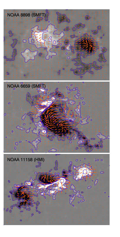
Figure 1: The vector magnetograms for three examples: NOAA 8898 (S13.0W7.0) observed by SMFT on 01:34 UT, March 8, 2000 (top); NOAA 6659 (N28.6W4.5) observed by SMFT on 05:29 UT, June 9, 1991 (middle); NOAA 11158 (S19.0E11.0) observed by HMI on 23:59 UT, Feb 14, 2011 (bottom). The arrows represent the direction of transverse field and the contours represent the longitudinal magnetic fields of $\pm 100,400,1600,3200G$.

By definition the current helicity is a scalar product of the magnetic field pseudo-vector and its curl (proportional to the electric current) vector. Generally speaking this construction can be obtained as a trace of a more generic three-index tensor quantity as it has been considered by Zhang et al. (2012), see their Appendix 1. For our analysis, let us denote local observable quantities by low cases, i.e. the local magnetic field ${\bf b}$ which is observable at the solar surface $z=0$ as well as the local electric current helicity density $h_{\rm c}={\bf b}\cdot{\rm curl\,}{{\bf b}}$. We denote $(x,y)$ local Cartesian coordinates on the image plane. The direction to the observer $z$ on the plane is fixed $z=0$. We reserve above mentioned notations $\bf B$ and $\chi$ for the magnetic field and current helicity in homogeneous and isotropic model. Then according to definition of ${\rm curl\,}$ this quantity naturally comprises of six parts: $\displaystyle\chi=\epsilon_{ijk}b_{i}\frac{\partial b_{k}}{\partial x_{j}}=h_{1}+h_{2}+h_{3}+h_{4}+h_{5}+h_{6}$ where

$$h_{1}=b_{z}\left(\frac{\partial b_{y}}{\partial x}\right); h_{2}=b_{z}\left(-\frac{\partial b_{x}}{\partial y}\right);$$

$$h_{3}=b_{x}\left(\frac{\partial b_{z}}{\partial y}\right); h_{4}=b_{x}\left(-\frac{\partial b_{y}}{\partial z}\right);$$ (3)

$$h_{5}=b_{y}\left(\frac{\partial b_{x}}{\partial z}\right); h_{6}=b_{y}\left(-\frac{\partial b_{z}}{\partial x}\right)\,.$$

We denote integral quantities over the available magnetogram field-of-view by capital cases $H_{i}=\int{h_{i}}dxdy$ for $i=1\,{\rm to}\,6$, so the overall average current helicity reads

$$H_{\rm c} = H_{1}+H_{2}+H_{3}+H_{4}+H_{5}+H_{6}$$

$$= \int b_{z}\left(\frac{\partial b_{y}}{\partial x}\right)dxdy+\int b_{z}\left(-\frac{\partial b_{x}}{\partial y}\right)dxdy$$

$$+ \int b_{x}\left(\frac{\partial b_{z}}{\partial y}\right)dxdy+\int b_{x}\left(-\frac{\partial b_{y}}{\partial z}\right)dxdy$$

$$+ \int b_{y}\left(\frac{\partial b_{x}}{\partial z}\right)dxdy+\int b_{y}\left(-\frac{\partial b_{z}}{\partial x}\right)dxdy\,.$$

Table 1: Summary of illustration computations of the helicity and boundary integrals in formula (5). The unit of $H_{1}$, $H_{6}$ and boundary integral is $10^{14}G^{2}m$.

Instr.	NOAA	date	Time	coordinate	$H_{1}$	$H_{6}$	$\%$ difference	bound.int.	err.est.
SMFT	8898	2000.03.08	01:37	S13.0W7.0	$-0.0493$	$-0.0495$	2.87%	0.0014	0.0135
SMFT	6659	1991.06.09	05:29	N28.6E4.5	$-1.4978$	$-1.4983$	0.31%	$-0.0046$	0.0306
HMI	11158	2011.02.14	23:47	S20W17	0.0793	0.0784	3.48%	$-0.0027$	0.0123

Using the integral by parts formula, we can obtain the following relation between helicity parts, for example,

$$\int b{z}\left(\frac{\partial b_{y}}{\partial x}\right)dxdy=\int b_{y}\left(-\frac{\partial b_{z}}{\partial x}\right)dxdy+\int\limits_{\Gamma}b_{z}b_{y}d{\it{l}}$$ (5)

where the latter integral is taken over contour $\Gamma$ at the boundary of our field of view (boundary integral). If we assume the magnetic field at the boundary of the active regions is weak enough, that means the boundary integral is very small, then the averages of the corresponding parts helicity are approximately equal in pairs $H_{1}\simeq H_{6}$ and $H_{2}\simeq H_{3}$. We illustrate validity of this consideration below.

For the purpose of illustration of our data we selected two active regions observed by SMFT in 1999 and 2000, and one to compare with other instruments, we used the data for an active region observed by Helioseismic and Magnetic Imager onboard the Solar Dynamics Observatory (HMI/SDO) in 2011. Figure 1 shows the vector magnetograms for three active regions observed by SMFT and HMI/SDO. We can see that the magnetic field is nearly potential for NOAA 8898 and the magnetic field is strong helical for NOAA 6659. The spatial resolution of HMI is higher than SMFT. We calculated the integrals $H_{1}$ and $H_{6}$ and the boundary integrals in formula (5). The results are listed in Table 1. The boundary integral is about 2.87%, 0.31% and 3.48% of the mean value of $H_{1}$ and $H_{6}$ for active region NOAA 8898, 6659 and 11158 respectively. In order to estimate tolerable error in computation of the boundary integral we use the typical noise levels: 20 G in $B_{z}$ and 100 G in $B_{y}$. For example, active region NOAA 6659, the error is about 2.04% of the mean value of $H_{1}$ and $H_{6}$. The corresponding boundary integral is well below the error level. These observational examples show that the above assumption of validity of integration by parts works pretty well when the magnetic field at the boundaries of the field of view is weak, so the formula (5) of integration by parts results in these equalities. Therefore, we established on the basis of both theoretical consideration and observational illustration that the four parts of observable current helicity are equal by pairs to their counterparts: $H_{1}\approx H_{6}$ and $H_{2}\approx H_{3}$.

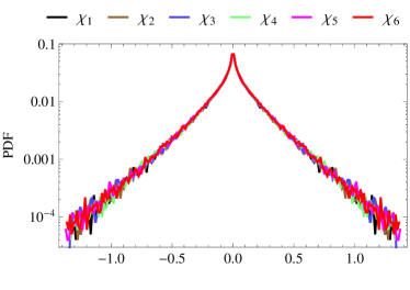
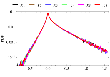
Figure 2: PDF for the six helicity parts: non-helical isotropic case (top), helical isotropic case (bottom). Note that only four out of the six are of observational interest. The x-axis is the relative value of helicity parts and the y-axis is the probability density function. All parts statistically coincide with each other though for the helical case there is a pronounceable bias visible as asymmetry over the center of distribution.

It is trivial to see that the local values of all helicity parts are generally unequal. Now let us consider whether the integral identities implied to mean helicity parts hold for the observational data.

First of all, all the parts of the total current helicity mentioned in the Introduction can be expressed in notations analogous to the ones in formulae (3) and their observational counterparts

$$\chi_{z}\,\,=\,\,\chi_{1}+\chi_{2}\,\,\,\longleftrightarrow\,\,\,H_{1}+H_{2}=H_{{\rm c}z}\,,$$

$$\chi_{x}\,\,=\,\,\chi_{3}+\chi_{4}\,\,\,\longleftrightarrow\,\,\,H_{3}+H_{4}=H_{{\rm c}x}\,,$$ (6)

$$\chi_{y}\,\,=\,\,\chi_{5}+\chi_{6}\,\,\,\longleftrightarrow\,\,\,H_{5}+H_{6}=H_{{\rm c}y}\,,$$

and notice that only the former part can be fully computed from observations as it does not contain derivatives with respect to $z$. Only one term in each of the two latter parts can be computed and the two terms $H_{4}$ and $H_{5}$ are not available from observations on the image plane. We either cannot use formula (5) for them as the relevant derivative is with respect to $z$ but integration is carried out over $x$ and $y$.

Let us assume local statistical isotropy of turbulence and take for instance two parts of helicity equal, say

$$\chi_{z}=\chi_{x}\,$$

Then we immediately have that as $H_{1}+H_{2}=H_{3}+H_{4}$, and due to formula (5) $H_{1}=H_{6}$ and $H_{2}=H_{3}$, then the three parts are equal

$$H_{1}=H_{4}=H_{6}\,.$$ (7)

Therefore, an additional assumption on the equality of the other helicity parts

$$\chi_{x}=\chi_{y}$$

would automatically lead to equality of the other three parts

$$H_{2}=H_{3}=H_{5}\,.$$ (8)

The above consideration means that for verification of the assumption of local isotropy unobservable parts of helicity $H_{4}$ and $H_{5}$ need to be evaluated in order to check equations (7-8).

Before doing further analysis we are going to see what relationship between the parts of helicity we can expect from theoretical consideration. For that purpose model simulation of the helicity parts is performed in the next section.

4 Simulations

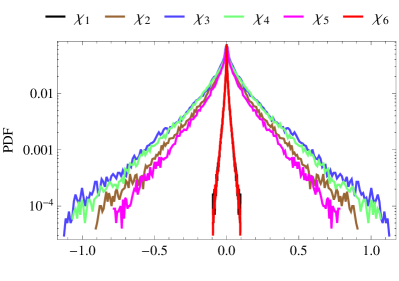
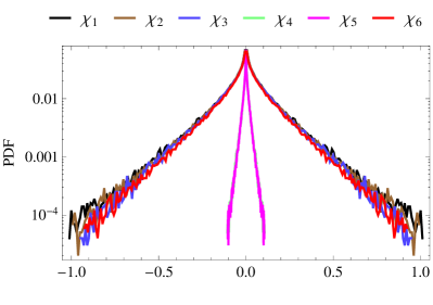
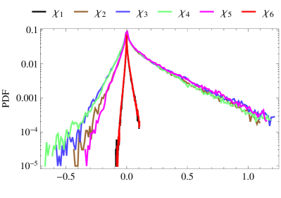
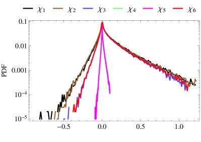
Figure 3: PDF for the six helicity parts same as in Figure 2: non-helical anisotropic case for anisotropy in $x$-direction (top left) and $z$-direction (top right), helical anisotropic case for anisotropy in $x$-direction (bottom left) and $z$-direction (bottom right).

Table 2: Summary of the model simulation cases partially presented on Figure 3. Note that observationally available parts of helicity are approximately equal in the case with anisotropy with respect to $z$ only. They are equal in all helical isotropic cases while in other anisotropic helical cases they are not equal.

case (mean $\pm$ dispersion)	$\chi_{1}$	$\chi_{2}$	$\chi_{3}$	$\chi_{4}$	$\chi_{5}$	$\chi_{6}$
Isotopic Non-helical	0.$\pm$2.71	0.$\pm$2.74	0.$\pm$2.62	0.$\pm$2.61	0.$\pm$2.67	0.$\pm$2.67
Isotropic Helical	1.56$\pm$3.12	1.53$\pm$3.12	1.53$\pm$3.11	1.55$\pm$3.12	1.56$\pm$3.12	1.56$\pm$3.11
Anisotropic-$x$ Non-helical	0.$\pm$0.19	0.$\pm$1.93	0.$\pm$2.28	0.$\pm$2.13	0.$\pm$1.79	0.$\pm$0.19
Anisotropic-$y$ Non-helical	0.$\pm$1.81	0.$\pm$0.2	0.$\pm$0.2	0.$\pm$1.88	0.$\pm$2.08	0.$\pm$2.14
Anisotropic-$z$ Non-helical	0.$\pm$2.2	0.$\pm$2.13	0.$\pm$1.9	0.$\pm$0.2	0.$\pm$0.2	0.$\pm$1.82
Anisotropic-$x$ Helical	0.05$\pm$0.2	1.29$\pm$2.24	1.29$\pm$2.41	1.36$\pm$2.57	1.23$\pm$2.04	0.05$\pm$0.2
Anisotropic-$y$ Helical	1.29$\pm$2.35	0.07$\pm$0.22	0.07$\pm$0.22	1.38$\pm$2.34	1.25$\pm$2.44	1.29$\pm$2.54
Anisotropic-$z$ Helical	1.26$\pm$2.44	1.26$\pm$2.47	1.26$\pm$2.19	0.06$\pm$0.2	0.06$\pm$0.2	1.26$\pm$2.18

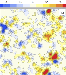
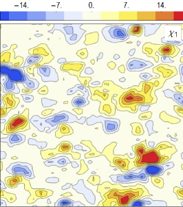
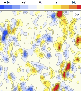
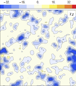
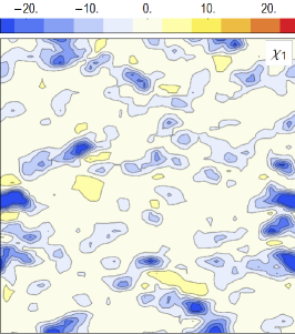
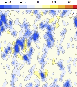
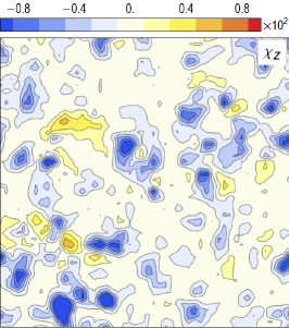
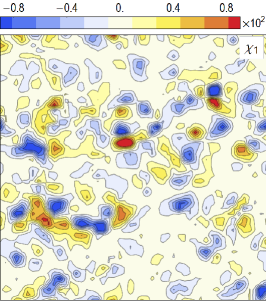
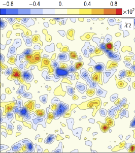
Figure 4: Distribution of $\chi_{z}$, $\chi_{1}$ and $\chi_{2}$ for three cases: non-helical magnetic field (top), helical magnetic field (middle), helical magnetic field plus potential magnetic field (bottom).

To prescribe a quasi-random magnetic field ${\mathbf{B}}$ with vanishing mean value in a periodic box, we use a Fourier expansion in modes with randomly chosen directions of wave vectors ${\mathbf{k}}$ but with amplitudes adjusted to reproduce any desired energy spectrum:

$${\mathbf{B}}({\mathbf{x}})=\frac{1}{(2\pi)^{3/2}}\int\hat{{\mathbf{B}}}({\mathbf{k}})e^{\mathrm{i}{\mathbf{k}}\cdot{\mathbf{x}}}\,\mathrm{d}^{3}{\mathbf{k}},$$ (9)

where $\hat{{\mathbf{B}}}$ is the Fourier transform of ${\mathbf{B}}$. The corresponding magnetic energy spectrum is given by

$$M(k)=\int_{|{\mathbf{k}}^{\prime}|=k}|\hat{{\mathbf{B}}}({\mathbf{k}}^{\prime})|^{2}\,\mathrm{d}^{3}{\mathbf{k}}^{\prime},$$ (10)

where the integral is taken over the spherical surface of radius $k$ in $k$-space. In the isotropic case, $M(k)=4\pi k^{2}|\hat{{\mathbf{B}}}(k)|^{2}$. In order to ensure periodicity within a computational box of size $L$, as required for the discrete Fourier transformation, the components of the wave vectors are restricted to be integer multiples of $2\pi/L$.

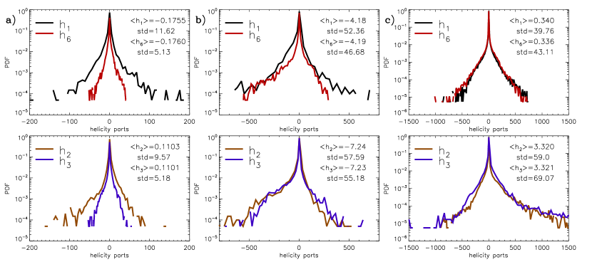
Figure 5: The examples of PDFs for the four observable helicity parts: a) column is for NOAA 8898; b) column is for NOAA 6659; c) column is for NOAA 11158. The upper (bottom) panels are the PDFs for helicity parts $h_{1}$ and $h_{6}$ ($h_{2}$ and $h_{3}$). The mean values and the standard deviations of helicity parts are given on the top right corner of each panel.

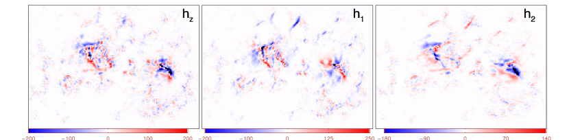
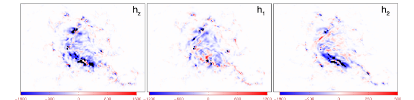
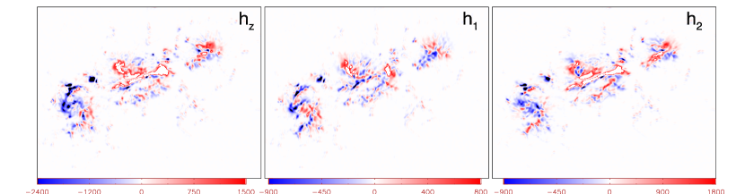
Figure 6: Distribution of $h_{z}$, $h_{1}$ and $h_{2}$ for the three examples: Nearly potential magnetic field in NOAA 8898 (top), helical magnetic field in NOAA 6659 (middle), relatively high special resolution magnetic field in NOAA 11158. The unit of helicity is $10^{-3}G^{2}/m$.

A solenoidal vector field ${\mathbf{B}}$, i.e., that having ${\mathbf{k}}\cdot\hat{{\mathbf{B}}}({\mathbf{k}})=0$, is specified by

$$\hat{{\mathbf{B}}}({\mathbf{k}})=\frac{{\mathbf{k}}\times{\mathbf{X}}}{|{\mathbf{k}}\times{\mathbf{X}}|}k^{-1}\sqrt{M(k)}.$$

Random choice a complex vector ${\mathbf{X}}$ implies zero net current helicity of ${\mathbf{B}}$. We consider a magnetic energy spectrum represented by two power-law ranges,

$$M(k)=M_{0}\left\{\begin{array}[]{ll}(k/k_{0})^{s_{0}}&\mbox{for }k<k_{0},\\ (k/k_{0})^{-s_{1}}&\mbox{for }k\geq k_{0},\end{array}\right.$$ (11)

with $s_{0}>0$, $s_{1}>0$ and $M_{0}=1$, where $k_{0}=6$ is the energy-range wave-number. We use $s_{1}=5/3$ as in Kolmogorov’s spectrum (Kolmogorov, 1941) and $s_{0}=2$ as in Christensson et al. (2001).

The helical ${\mathbf{B}}$ can be obtained with choice ${\mathbf{X}}$ as

$${\mathbf{X}}={\mathbf{Y}}\pm\mathrm{i}|{\mathbf{Y}}|\frac{{\mathbf{k}}\times{\mathbf{Y}}}{|{\mathbf{k}}\times{\mathbf{Y}}|},$$ (12)

where the sign defines the sign of current helicity and ${\mathbf{Y}}({\mathbf{k}})={\mathbf{Y}}(-{\mathbf{k}})$ is a random real vector. Condition (12) implies $\hat{{\mathbf{B}}}({\mathbf{k}})=\hat{{\mathbf{B}}}^{*}(-{\mathbf{k}})$.

The probability density functions (PDFs) calculated from 2D distributions [$(x,y)$-plane of 3D simulated cube] are shown in Fig. 2. First of all we note that isotropy means similarity of distributions of $\chi_{1}$, $\chi_{2}$, $\chi_{3}$ and $\chi_{6}$. Secondly, non-zero helicity leads to asymmetry of PDFs. Furthermore, we can produce corresponding statistically anisotropic fields for non-helical and helical cases.

Anisotropic case is simulated by the additional factor in $M(k)$. One can take

$$M(k)=k_{x}^{-2}M_{0}\left\{\begin{array}[]{ll}(k/k_{0})^{s_{0}}&\mbox{for }k<k_{0},\\ (k/k_{0})^{-s_{1}}&\mbox{for }k\geq k_{0},\end{array}\right.$$ (13)

The corresponding PDFs are shown in Figure 3. From Figure 3 one can see that anisotropy in different direction affects the PDFs of different parts of helicity in a different way. Anisotropy in $x$-direction on the left two panels leads to the parts of helicity $\chi_{1}$ and $\chi_{6}$ containing derivatives in this direction to be distributed with much lower dispersion. One can see the same for anisotropy in $z$-direction in the right panels for $\chi_{4}$ and $\chi_{5}$. Each of the two quantities in these pairs are distributed statistically similar. For the remaining parts of helicity, in the helical case (bottom panels), we can see that the left and right tails of the PDFs have different spreads and in particular the left tails are more inclined. Furthermore, we see that these four remaining parts of helicity group in two statistically similar pairs, with respect to the component of the magnetic field which enters into each of the parts, namely $B_{x}$ for $\chi_{3}$ and $\chi_{4}$ in case of anisotropy in $x-$ direction and $B_{Z}$ for $\chi_{1}$ and $\chi_{2}$ in case of anisotropy in $z-$direction.

The results for the cases shown in Figure 3 are summarized in Table 2. One can see that the mean values of the six helicity parts are approximately equal in the isotropic helical case. In the anisotropic helical cases, in accord with the integration by parts formula (5), the mean values of helicity parts are equal in pairs: $\langle\chi_{1}\rangle\approx\langle\chi_{6}\rangle$ and $\langle\chi_{2}\rangle\approx\langle\chi_{3}\rangle$. The other two parts $\langle\chi_{4}\rangle$ and $\langle\chi_{5}\rangle$ are not subject of the formula (5) as they contain derivatives with respect to $z$ while averaging involves differentiation over the image plane $(x,y)$, and they may generally be different, as it is in the anisotropic helical case.

Now let us consider how the sign of the parts $\chi_{1}$, $\chi_{2}$, $\chi_{3}$ and $\chi_{6}$ can locally represent the sign of the total helicity. One effect can be the contribution from the potential magnetic field. We simulate distributions of $\chi_{z}$, $\chi_{1}$ and $\chi_{2}$ for three cases: non-helical magnetic field, helical magnetic field and helical magnetic field plus potential magnetic field (see Figure 4 from top to bottom). As expected for the purely non-helical magnetic field, the all three maps possess the same kind of patterns with alternating sign. For the helical case we also have the same kind of patterns but with dominating sign of helicity. Additional contribution from the potential magnetic field does not change much the total helicity $\chi_{z}$ but its parts $\chi_{1}$ and $\chi_{2}$ have strongly alternating pattern unlike for the case of non-helical magnetic field. We can see that assigning these two parts the opposite signs in the alternating pattern may merely cancel each other.

Therefore, we have seen that the four parts of helicity that have observational interest are close in pairs, but between the pairs there may be a significant difference in their distributions and the integral values. We have also noted now the specific contribution of one and the other parts may partially cancel each other in the overall helicity.

5 Observational Results

Now we compare theoretical predictions with results of observational data analysis. Figures 5 show PDFs for the four observationally available parts of helicity $h_{1}$, $h_{2}$, $h_{3}$, $h_{6}$ computed for all pixels in the magnetograms of the three active regions shown in Figures 1. One can see that the mean values of distribution for pair ($h_{1}$, $h_{6}$), and pair ($h_{2}$, $h_{3}$) are very close to each other with accuracy of a few per cent, but the difference between the mean values of $h_{1}$ and $h_{2}$ ($h_{3}$ and $h_{6}$) is large although the distribution pattern is similar. This observational result is similar with the anisotropic case simulation in Figure 3 although some difference is found. This discrepancy can be attributed to the complexity of the observation. We also show the distribution map for $h_{z}$, $h_{1}$ and $h_{2}$ in Figure 6. We can see that there is a significant difference in the distribution of $h_{1}$ and $h_{2}$, but their sum is nearly equal to $h_{z}$.

We have analyzed similar distributions for various vector magnetograms obtained at Huairou Solar Observing Station (HSOS) available for date in cycles 22 and 23 as well as a recent vector magnetograms observed by HMI/SDO in order to learn that the properties above for this PDF is quite generic for the magnetograms under consideration.

Now from the study of distribution of the parts of helicity by pixels over a given magnetogram of an active region we move towards study the distribution of the mean values of these quantities for 6629 magnetograms observed by HSOS from 1988 to 2005.

Figure 7 shows scatter plots for helicity parts for our sample. One can see that correlation between $H_{1}$ and $H_{6}$ ($H_{2}$ and $H_{3}$) is very high while the one between $H_{1}$ and $H_{2}$ ($H_{3}$ and $H_{6}$) is low. This means that average with signed flux $b_{z}$ weighted by $\displaystyle{-\frac{\partial b_{x}}{\partial y}}$ is systematically different from the one weighted by $\displaystyle{-\frac{\partial b_{y}}{\partial x}}$ in a magnetogram. These confirm that the properties which we see above for the PDFs of helicity parts in a magnetogram: robustness of numerical scheme for the use of integration by parts, as well as absence of isotropy. Comparing with our theoretical simulation in the section above, this statistical observational result corresponds to anisotropic helical case while anisotropy is either by $x$ or $y$, or both. This is not the case of purely anisotropic by only vertical $z$-direction (convective stratified turbulence). We also studied the sign agreement between helicity parts. We found that 95.5% (95.9%) of $H_{1}$ and $H_{6}$ ($H_{2}$ and $H_{3}$) among 6629 vector magnetograms agree in their signs, while for $H_{1}$ and $H_{2}$ ($H_{3}$ and $H_{6}$) the percent of agreement is much lower which is 38.0% (34.7%). We checked the vector magnetograms whose $H_{1}$ and $H_{6}$ ($H_{2}$ and $H_{3}$) have different sign and found that the magnetic fields are not weak at the boundary for some of those magnetograms. On the other hand, the values of helicity parts inferred from those magnetograms are often smaller by one or two orders of magnitude than for the typical magnetograms. Those values are too small to be estimated accurately.

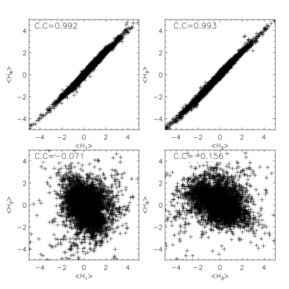
Figure 7: Scatter plots key helicity parts over the dataset 1988-2005. each point represents average value of helicity parts for one magnetogram. The unit of helicity is $10^{-3}G^{2}/m$.

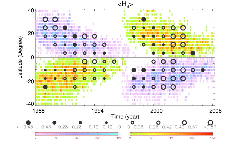
Figure 8: Evolution of four helicity parts with the solar cycle overlaid with sunspot density (color). The vertical axis gives the latitude and the horizontal axis gives the time in years. The circle size gives the magnitude of helicity as averaged over two-year running windows over latitudinal bins of $7^{\circ}$ wide. The unit of helicity is $10^{-3}G^{2}/m$.

Let us study how the local anisotropy of current helicity varies with the solar cycle. From Figure 8, we can see that the latitudinal structure and variation with the solar cycle of $\langle H_{1}\rangle$ and $\langle H_{6}\rangle$ ( $\langle H_{2}\rangle$ and $\langle H_{3}\rangle$) are identical except a small part which is different. The reasons for this difference are analyzed in the above paragraph. While the latitudinal structure and variation with the solar cycle of $\langle H_{1}\rangle$ and $\langle H_{2}\rangle$ ( $\langle H_{3}\rangle$ and $\langle H_{6}\rangle$) are much different which confirms again the absence of isotropy for the observable current helicity in solar active regions. We can also see that in some periods and latitudinal intervals the helicity parts satisfy the hemispheric sign rule (negative/positive sign in the North/South hemispheres) well, e.g., 1992–1994 and 2001–2003 for $\langle H_{1}\rangle$ in southern hemisphere. The fractions of magnetograms following the hemispheric sign rule are 46.2% for $\langle H_{1}\rangle$, 61.9% for $\langle H_{2}\rangle$, 60.2% for $\langle H_{3}\rangle$ and 47.2% for $\langle H_{6}\rangle$ in northern hemisphere respectively, while in southern hemisphere they are 57.9% for $\langle H_{1}\rangle$, 55.4% for $\langle H_{2}\rangle$, 54.4% for $\langle H_{3}\rangle$ and 57.1% for $\langle H_{6}\rangle$ respectively.

The sum $\langle H_{cz}\rangle=\langle H_{1}\rangle+\langle H_{2}\rangle$ usually used in the past study in Figure 9 shows some anti-symmetry with respect to the solar equator and the hemispheric sign rule is well pronounced, this figure is almost the same as Figure 2 in Zhang et al. (2010). The use of the sum of the other two helicity parts $H_{6}$ and $H_{3}$, respectively, would produce visually identical result, and not shown here. The fractions of magnetograms following the hemispheric sign rule for $\langle H_{cz}\rangle$ are 58.9% in northern hemisphere and 61.7% in southern hemisphere respectively. We can see some regular inversions of hemispheric sign rule within isolate ranges of latitudes near the beginning and the end of the solar cycle for $\langle H_{cz}\rangle$. We note that during these phases the signs of pair of helicity parts ($\langle H_{1}\rangle$ and $\langle H_{2}\rangle$) are often the same and violate the hemispheric sign rule, which makes their joint contribution to the reversal of hemispheric sign rule.

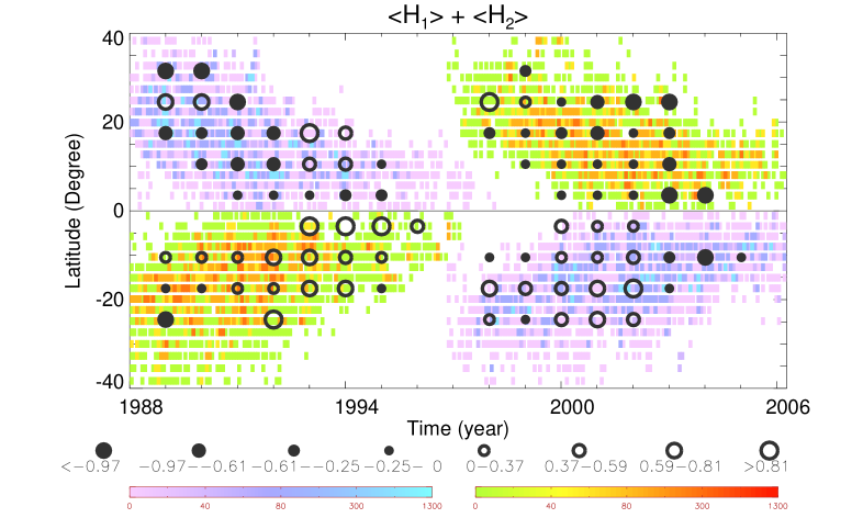
Figure 9: Evolution of the observationally available helicity defined as a sum of two parts $\langle H_{1}\rangle+\langle H_{2}\rangle$ with the solar cycle. The unit of helicity is $10^{-3}G^{2}/m$.

Table 3: Summary of the relative degree of anisotropy. The unit of $H_{1}$ and $H_{2}$ is $10^{14}G^{2}m$.

Instr.	NOAA	date	Time	coordinate	$H_{1}$	$H_{2}$	$q_{12}$	$q_{12}^{a}$
SMFT	8898	2000.03.08	01:37	S13.0W7.0	$-0.0493$	0.0310	0.8348	0.8325
SMFT	6659	1991.06.09	05:29	N28.6E4.5	$-1.4978$	$-2.5897$	0.7823	0.7794
HMI	11158	2011.02.14	23:47	S20W17	0.0793	0.7739	0.7472	0.7472

6 Discussion

In order to establish the degree of anisotropy quantitatively, we take 3 active regions which used for calculating boundary integral in section 3 for examples. We estimate the relative degree of anisotropy, for example, as a relative anisotropy imbalance between the two parts of helicity using some norm as following:

$$q_{12}={\|h_{1}-h_{2}\|\over\|h_{1}\|+\|h_{2}\|},$$ (14)

where the norm $\|h\|$ can be computed as

$$\|h\|=\sqrt{{\int(w|h|^{2}dxdy)\over\int(wdxdy)}},$$ (15)

where $w$ is weight factor as follow: when we integrate in the magnetogram using all pixels, then $w=1$. Alternatively, we can use only pixels where the signal is greater than cut-off noise levels ($|B_{z}|>20G$ and $B_{t}>100G$) as we usually do so in helicity statistical studies ($w=1$ if greater, or $w=0$ if less than noise level). The value of $q_{12}$ is between 0 to 1. The results are listed in Table 3. $q_{12}$ is calculated using all pixels in the magnetogram, $q_{12}^{a}$ is only using the pixels where the signal is greater than cut-off noise levels. From this table, the order of $q_{12}$ is from 0.74 to 0.83 and it is not affected much by the noise, which is close to 1, it says that the observed quantities are extremely anisotropic.

We may further speculate about the sources of anisotropy of current helicity. One effect which sounds trivial in the solar photosphere would be vertical stratification of convection. We, however, are inclined to discuss this issue as the parts of helicity involving vertical derivatives of the magnetic field are not observationally available. The difference in properties and behaviour of $H_{1}$ and $H_{2}$ is likely a manifestation of the effect of rotation as one contains derivatives with respect to azimuthal (collinear to rotation), and the other meridional direction (perpendicular to rotation). The other source of anisotropy could be the effect of large-scale magnetic field. Two components (azimuthal and radial) of the solar cyclic magnetic field are anti-symmetric over the equator and the other meridional component is symmetric over the solar equator.

The complete use of the assumption of local statistical isotropy means also the equality between these two groups of the three parts of helicity in equation 7 and 8. Two of them, $H_{4}$ and $H_{5}$, however, can not be calculated from the observational vector magnetograph data at the solar photosphere. Therefore, we can not check the condition of local isotropy of solar turbulence in active region by observationally available data completely. On the Other hand, there are several factors which affect the precision of the calculated helicity parts, such as that the accuracy of transversal field is lower than the one of longitudinal field, the magneto-optical effects, calibration of magnetic fields etc. We cannot completely estimate the influence of these factors on the helicity parts although we used some data reduction method to reduce it. This topic requires further investigation.

7 Conclusion

We have studied the distribution and properties of the parts of current helicity from observation and simulation. The main conclusions are as following:

(1) The simulation results show that the means of the six helicity parts statistically coincide with each other for the isotropic case, while for the anisotropic helical case it is different.

(2) The distribution of the observed helicity parts is similar with the helical anisotropic case in simulations. This shows that the distribution of the observed helicity parts is anisotropic over active region scales. Assumptions of local homogeneity and isotropy in computation of observational proxies of helicity require further analysis in the light of our findings.

(3) The four observable helicity parts are equal in pairs owing to the magnetic field is weak at the boundaries of magnetogram, but there is a large difference between different pairs which may be caused by the anisotropy of the current helicity density in active region. Both the pairs of the helicity parts follow the hemispheric sign rule with certain exceptions in periods and hemispheres but the sums of the two parts follow the hemispheric sign rule more robust and uniform than the individual parts of helicity alone.

More theoretical modeling of anisotropy in solar-like turbulence is required to understand these statistical results. Our simple simulations have shown that the anisotropy may be present in several directions and not only in the direction of vertical stratification. This is confirmed by several examples of observational data as well as their statistical analysis. Other sources of anisotropy such as inhomogeneity or rotation, and furthermore presence of the large-scale mean magnetic field which alternates in sign with every 11-year sunspot cycle may be possible explanations of these results.

References

- Abramenko et al. (1996) Abramenko, V.I., Wang, T.J., Yurchishin, V.B., 1996, Sol. Phys. 168, 75.
- Ai & Hu (1986) Ai, G.X., Hu, Y.F., 1986, Acta Astron. Sinica 27, 173.
- Bao & Zhang (1998) Bao, S.D., Zhang, H.Q., 1998, ApJ 496, L43.
- Babcock (1961) Babcock, H., 1961, ApJ, 133, 572.
- Berger (2003) Berger M. A., 2003, in Ferriz-Mas, A., Núñez, M. (eds.), Advances in Nonlinear Dynamics, Taylor and Francis Group, London, 345.
- Berger and Field (1984) Berger M. A., Field G. B., 1984, J. Fluid. Mech. 147, 133.
- Brown et al. (1999) Brown M., Canfield R., Pevtsov A., 1999, Magnetic Helicity in Space and Laboratory Plasmas, Geophys. Mon. Ser. 111, AGU.
- Christensson et al. (2001) Christensson, M. and Hindmarsh, M. and Brandenburg, A. Phys. Rev. E 64, 056405 (2001).
- Dupont et al. (2007) Dupont, J.-C., Schmidt, F., Koutny, P., 2007, Sol. Phys. 323, 965.
- Gao et al. (2008) Gao, Y., Su, J., Xu, H. and Zhang, H., 2008, Mon. Not. R. Astron. Soc., 386, 1959.
- Goldreich and Sridhar (1997) Goldreich P., Sridhar S., 1997, ApJ 485, 680.
- Hagino and Sakurai (2004) Hagino, M., Sakurai, T.: 2004, PASJ 56, 831.
- Iroshnikov (1963) Iroshnikov, P. S. 1963, AZh, 40, 742
- Kolmogorov (1941) Kolmogorov, A.N., 1941, Dokl. A N SSSR, 30, 299
- Kraichnan (1965) Kraichnan, R. H. 1965, Phys. Fluids, 8, 1385
- Leighton (1969) Leighton, R., 1969, ApJ, 156, 1.
- Parker (1955) Parker, E., ApJ 122, 293.
- Pevtsov (1994) Pevtsov, A.A., Canfield, R.C., Metcalf, T.R., 1994, ApJ, 425, L117.
- Seehafer (1990) Seehafer, N. 1990, Sol. Phys. 125, 219.
- Wang, Xu, and Zhang (1994) Wang T.J., Xu A.A., Zhang H.Q. 1994, Sol. Phys., 155, 99.
- Zhang et al. (2010) Zhang Hongqi, Sakurai T., Pevtsov A, Gao Yu , Xu Haiqing, Sokoloff D. D. and Kuzanyan K., 2010, Mon. Not. R. Astron. Soc. 402, L30.
- Zhang et al. (2012) Zhang H., Moss D., Kleeorin N., Kuzanyan K., Rogachevskii I., Sokoloff D., Gao Y., and Xu H., 2012, ApJ 751, 47.