Rapid Computation of Thermodynamic Properties Over Multidimensional Nonbonded Parameter Spaces using Adaptive Multistate Reweighting

Abstract

We show how thermodynamic properties of molecular models can be computed over a large, multidimensional parameter space by combining multistate reweighting analysis with a linear basis function approach. This approach reduces the computational cost to estimate thermodynamic properties from molecular simulations for over 130,000 tested parameter combinations from over a thousand CPU years to tens of CPU days. This speed increase is achieved primarily by computing the potential energy as a linear combination of basis functions, computed from either modified simulation code or as the difference of energy between two reference states, which can be done without any simulation code modification. The thermodynamic properties are then estimated with the Multistate Bennett Acceptance Ratio (MBAR) as a function of multiple model parameters without the need to define a priori how the states are connected by a pathway. Instead, we adaptively sample a set of points in parameter space to create mutual configuration space overlap. The existence of regions of poor configuration space overlap are detected by analyzing the eigenvalues of the sampled states’ overlap matrix. The configuration space overlap to sampled states is monitored alongside the mean and maximum uncertainty to determine convergence, as neither the uncertainty or the configuration space overlap alone is a sufficient metric of convergence.

This adaptive sampling scheme is demonstrated by estimating with high precision the solvation free energies of charged particles of Lennard-Jones plus Coulomb functional form with charges between -2 and +2 and generally physical values of $\sigma_{ij}$ and $\epsilon_{ij}$ in TIP3P water. We also compute entropy, enthalpy, and radial distribution functions of arbitrary unsampled parameter combinations using only the data from these sampled states and use the estimates of free energies over the entire space to examine the deviation of atomistic simulations from the Born approximation to the solvation free energy.

1 Introduction

Many applications of molecular simulations require searching over large parameter spaces to predict or match physical observables. Molecular simulation parameters such as charges, Lennard-Jones dispersion and repulsion parameters, as well as bonds, angles, and torsion force constants determine the energies and probabilities of configurations in simulations, and thus in turn, determine what thermodynamic properties will be observed. The ability to accurately estimate thermodynamic properties without the need for laboratory experiments has the potential to save both time and resources in fields such as polymer ¹ and solvent ² design as well as drug discovery. ^{3, 4, 5} This time and cost savings is important both in the design of new molecules, where properties are unknown, and ’reverse property prediction’ where a model or molecule is designed to match specific experimental targets, such as designing metal-organic frameworks (MOFs) with specific gas loadings. ⁶

Assigning proper parameters in a molecular simulation given a set of experimental data becomes more difficult as the number of free parameters increases. Some experimental parameters, such as bond lengths and angles, are relatively easy to estimate using small-molecule crystallographic structures and quantum chemistry. However, nonbonded parameters, such as partial charges and dispersion terms, are much more difficult to choose as they are model parameters that do not directly correspond to laboratory observables such as bond length. Instead, possible nonbonded parameters are constrained by sets of experimental observables such as transfer free energies, heats of vaporization, densities, and heat capacities.

Identifying nonbonded model parameters consistent with a set of experimental thermodynamic values requires expensive iterative, self-consistent simulations or even more expensive gradient optimizations. ⁷ Most condensed phase force fields ^{8, 9, 10, 11, 12, 13, 14} are parameterized by manual iterative fitting to a training set of experimental thermodynamic data for a small set of molecules chosen to represent a broader spectrum of similar molecules. ^{15, 16} Accurate fits are required to predict properties of biological systems or complex mixtures where group contribution methods such as UNIQUAC ¹⁷ and UNIFAC ¹⁸ are inadequate.

Some of the most computationally expensive properties to estimate involve the free energy differences between two states, such as the solvation free energy, which is the free energy difference of two systems as one solute molecule moves from solution to vapor, or activity coefficients, which measure the deviation of the chemical potential of a species from ideality. Accurately computing free energy differences (or equivalently, chemical potential differences) also provide a way to compute many other thermodynamic properties as they can be derived from the derivatives of the free energy with respect to temperature ($T$), pressure ($P$), volume ($V$), and number of particles ($N_{i}$).

Estimating free energy differences between two thermodynamic states accurately requires designing a thermodynamic path between the states. Paths that are both computationally and statistically efficient, especially for full deletion or insertion of a molecule into a dense fluid, are nontrivial to design and must often include a number of non-obvious, nonphysical intermediates. ^{19, 20, 21, 22, 23, 24, 25, 26, 27, 28, 29, 30, 31, 32, 33} The end states and multiple intermediate states along the thermodynamic path must be sampled to create good configuration space overlap between the end states, which is required to accurately estimate free energy differences between the endpoints. ^{34, 35, 19, 36, 37, 5} Technically, we require good overlap in the full phase space, both configurations and velocity, but because velocities are thermalized in essentially all systems of thermodynamic interest, it is the configuration space that we must generally worry about when connecting states together.

If one wishes to compute free energies of solvation for many different parameterizations of the same molecule, the direct approach of calculating an entire thermodynamic pathway for each parameter choice is extremely expensive for highly accuracy calculations. Additionally, examining the differences in free energies due to a small change of parameters is particularly difficult because we must take the differences between two similar numbers with independent statistical error.

Reweighting methods can help solve both the problem of expense and the problem of cancellations of errors. In a recent study, our group showed how multistate reweighting can directly calculate the $\Delta\Delta G$ between two different long-range interaction approaches, with very small uncertainties for relatively low computational cost. ³⁸ The expense is lowered by constructing thermodynamic cycles directly connecting Hamiltonians with similar parameters and thus significantly overlapping configurational spaces. These small uncertainties are possible because MBAR can directly calculate the covariances between the two free energies through analyzing all potential energy differences, rather than only uncorrelated calculations. This same approach can be applied to small changes in parameters.

Estimating properties with reweighting methods requires constructing a thermodynamic path between the different parameterizations. It also requires potentially significant computational resources to perform simulations with parameters that have properly overlapping configurations. The combination of these two requirements adds theoretical and practical limitations to simultaneously searching large, multidimensional nonbonded parameter spaces.

1. The space of nonbonded parameters is often at least multiple dimensions per particle or particle type. For example, the nonbonded parameters of charge ($q$) and least two Lennard-Jones-like terms ($\epsilon_{ij}$, $\sigma_{ij}$) can result in at least three parameter dimensions per particle type.

2. There is no obvious way to define computationally efficient thermodynamic paths between any two points in these multidimensional spaces or select a prior simulation points in this space that give rise to low error estimates of thermodynamic properties across the entire space.

3. Reweighting methods requires computing energies from the sampled configurations to other sampled states, and any unsampled state of interest. This re-computation typically requires re-running the simulation force loops over all generated configurations for each combination of parameters of interest. The computational cost to search such a multidimensional space of nonbonded parameters scales, at best, linearly with the number of samples, and at worst quadratically with the number parameter combinations, since data may be collected with simulations at each parameter combination. ²⁹

Designing efficient thermodynamic paths through arbitrary thermodynamic states is a challenging task, ^{27, 29, 30} but designing paths in multidimensional parameter spaces adds additional complexities. An example in Fig. 1 demonstrates the challenges of identifying low-uncertainty paths in multiple dimensions. This figure shows two arbitrarily defined thermodynamic states in a two-dimensional parameter space and attempts to draw pathways between them with high mutual configuration space overlap, providing low error estimates. However, the choice of which path to sample to connect the states is not immediately obvious. The shortest Euclidean path in parameter space has large uncertainty, but two alternative paths have low uncertainty. This sort of multidimensional space raises questions with no obvious answers: How can we a priori identify which paths have more mutual overlap (i.e. result in simulations with lower uncertainty) without exhaustively sampling the system? Could samples drawn from both paths but with different proportions provide lower uncertainty than sampling either path by itself?

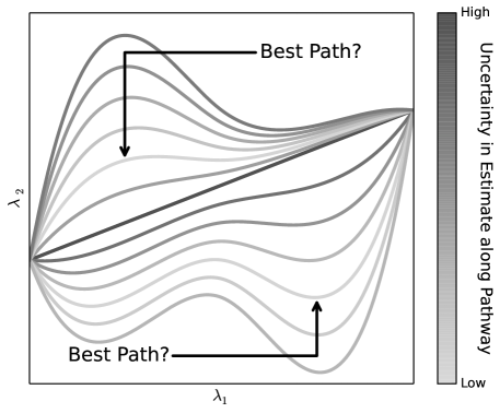
Figure 1: Defining the “best” thermodynamic path between arbitrary states is a nontrivial problem. This figure shows several multidimensional thermodynamic paths connecting two states, and the relative uncertainty of each pathway shown by a gray scale gradient of each curve. The path with shortest Euclidean distance in parameter space ($\lambda_{1}$, $\lambda_{2}$) has a large uncertainty, and at least two of the other paths have lower uncertainty. However, it is unclear if sampling a single “best path,” or a combination of multiple low variance paths will have the highest computational efficiency for a target statistical error. The most computationally efficient sampling scheme may not be along any single path at all, and instead may be achieved by sampling a non-parameterized states in a multidimensional parameter space.

Previous research on identifying low-variance paths along a single coupling parameter used local minimization of total variance along the path. ^{27, 29, 30} However, in multiple dimensions, since multiple potential low-variance paths could exist, local optimization is unlikely to identify the most efficient path between states of interest, nor whether it would be more optimal to traverse both paths. The identification of an optimal path choice is made more complicated if we are interested in all the mutual free energy differences between multiple states, since we must identify a path or a network of paths connecting all of the states, with samples collected along each of these states. One would ideally want ad hoc rules estimating the computational efficiency of these paths, determined a priori to avoid unnecessary sampling. Defining such rules for a diverse set of chemical systems becomes increasingly complex as the dimensionality and the number of states increases. Removing the need to define these difficult multidimensional paths significantly lowers these barriers to searching through large parameter spaces for optimal parameters.

We can remove the need to explicitly define thermodynamic paths between states in multiple dimensions with multistate reweighting methods. These methods, such as the Multistate Bennett Acceptance Ratio (MBAR) ³⁹ and the Weighted Histogram Analysis Method (WHAM), ^{40, 41} allow analyzing samples from anywhere in the parameter space to compute properties anywhere else in the space, without the need to define which thermodynamic states are adjacent as is needed for the original Bennett Acceptance Ratio (BAR). ³⁵ MBAR has the important advantage over WHAM in that sampled configurations do not need to be binned along a pre-defined thermodynamic path for the analysis which is particularly important in multidimensional spaces, where it becomes increasingly difficult to populate histogram bins. Any given combination of nonbonded parameters will share a high degree of configuration space overlap with a large number of similar parameter sets, though it is not always clear a priori which ones those will be. MBAR takes into account all of the information from all sampled states in determining the free energy differences between any two states, sampled or unsampled. Therefore, with moderate sampling at the right parameter combinations, thermodynamic properties can be estimated at a large number of parameter combinations, even without explicit sampling of every parameter combination, so long as for each choice of parameters there is some degree of configuration space overlap with some combination of sampled parameters.

With the limitation of explicitly defining a thermodynamic path removed, we can focus on decreasing the computational cost of gathering the statistical information required for multistate reweighting calculations of thermodynamic information. Reweighting methods require the energy of each sampled configuration to be known at each state of interest to compute free energy differences and other properties between states. Computing a configuration’s energy multiple times with different energy functions is a time limiting step for calculating thermodynamic properties across large parameter spaces. Collecting the energy of each configuration at each state usually requires running the simulation code, or at least the inner force loop of simulation code, multiple times on each configuration. If we only are interested in reweighting the properties from a single sampled state ⁴², we would only have to carry out this computation once per configuration ($N$) generated at a sampled state ($K_{s}$), per unsampled state of interest ($K_{u}$). This results in energy calculations that scale as $\mathcal{O}\left(N(K_{u}+K_{s})\right)$, assuming equal sampling per sampled state. However, such estimates are known to be statistically inefficient and prone to substantial bias when overlap is not substantial. ^{43, 44, 45} Multistate methods, like MBAR, ³⁹ require calculating the energy for each configuration at each sampled state as well as each state of interest, so the scaling is quadratic in the number of sampled states as $\mathcal{O}\left(N(K_{u}+K_{s}^{2})\right)$. This is not a burdensome task for a small number of states along a single thermodynamic path, making it well worth using multistate simulations regardless of how expensive recalculating the energies of this configurations are. However, as tens or hundreds of thousands of states of interest and hundreds of sampled states are considered, this scaling becomes a computational bottleneck that must be overcome.

We can reduce the cost to compute energies at thermodynamic states to computationally trivial vector multiplication by defining the energies using linear basis functions. ^{26, 29, 30} Energies calculated using a basis function approach can be most generally written by

$$u(r,\lambda)=\sum_{i}^{n}h_{i}(\lambda)u_{i}(r)+u_{\text{unaffected}}(r)$$ (1)

where $u(r,\lambda)=\beta U(r,\lambda)$ is the reduced energy as a function of both the configuration $r$ and some (possibly multidimensional) alchemical coupling parameter $\lambda$; $h_{i}(\lambda)$ are a set of nonphysical, alchemical switches that are independent of configuration; $u_{i}(r)$ are the basis functions; $n$ is the total number of basis function and alchemical switch pairs; and $u_{\text{unaffected}}(r)$ is the system’s potential energy not dependent on the alchemical variables. This approach computes the energy of a configuration at any thermodynamic state by scalar multiplication of the configuration dependent basis functions, which only have to be computed once per configuration. The vector multiplication can eliminate the need to run the inner force loop on a configuration more than once, reducing the computational cost of evaluating energies from $\mathcal{O}\left(N(K_{u}+K_{s}^{2})\right)$, to $\mathcal{O}\left(NK_{s}\right)$, which is simply the total number of sampled configurations. The alchemical switches can take any form, so long as $r$ remains part of the basis functions and not the switches. This form of the potential energy is in contrast to forms such as the soft core form of repulsive interactions ^{46, 47}, which cannot be represented as sums of separable combinations of $r$ and $\lambda$.

In this study we combine multistate reweighting methods with a linear basis function approach to compute thermodynamic properties over a large nonbonded parameter space. To demonstrate the process, we look at the Lennard-Jones parameters $\epsilon_{ii}$ and $\sigma_{ii}$, and partial charge, $q_{i}$, for a single particle in explicit solvent. This approach could can aid in future large parameter space searches to quickly find a range of nonbonded parameters and fine tune a fitting or optimization procedure. The relative free energy, enthalpy, and entropy of solvation are explored as these are some of the most computationally expensive properties to estimate. We also estimate the Born solvation free energy of charging, compare our results to specific ion free energies computed from others, and compute radial distribution functions. The techniques shown here are generalizable to other thermodynamic properties.

We explore both a two-dimensional and a three-dimensional parameter space. A 2-D parameter space in $\epsilon_{ii}$ and $\sigma_{ii}$ is first explored as a test of searching through parameter space. A larger, 3-D parameter space in $\epsilon_{ij}$, $\sigma_{ii}$, and $q_{i}$ is then also explored and iterative simulations are carried out to reduce the statistical error in the estimate of solvation properties across the entire range of parameters.

2 Theory

The notation in this study is as follows. $\sigma_{ii}$ and $\epsilon_{ii}$ are the Lennard-Jones parameters, and $q$ is the charge of a particle. $\epsilon_{0}$ is the permittivity of vacuum. $u(r)$ are basis functions of the potential energy function and $h(\lambda)$ are the alchemical switches. Subscripts $E$, $R$, and $A$ denote an electrostatic, Lennard-Jones repulsive, and Lennard-Jones attractive term respectively, e.g. $u_{E}(r)$ is the electrostatic basis function. The subscripts $i$, $j$, and $k$ on nonbonded parameters denote arbitrary atoms, and subscripts $X$, $Y$, and $Z$ denote an explicit set of parameters which define a thermodynamic state. and have fixed values but not explicitly defined to be general. Subscript $S$ denotes a solvent particle. The subscript $\ell\,$ will be used for summation indices, and $C$ represents a collection of constants.

2.1 Representing nonbonded parameter space with basis functions

We generalize the potential energy to simplify writing the energy of any potential in multidimensional space. The three nonbonded parameters explored here lead to a pairwise nonbonded potential energy between two point particles a distance $r$ apart

$$u(r)=\frac{4\epsilon_{ij}\sigma_{ij}^{12}}{r^{12}}+\frac{-4\epsilon_{ij}\sigma_{ij}^{6}}{r^{6}}+\frac{q_{i}q_{j}}{4\pi\epsilon_{0}r}\text{.}$$ (2)

Eq. (2) can be more generally written as

$$u(r) =\frac{C_{12}}{r^{12}}+\frac{C_{6}}{r^{6}}+\frac{C_{1}}{r}$$ (3)

$$=\sum_{\ell}\left(\frac{C_{n}}{r^{n}}\right)_{\ell}$$ (4)

where $n$ takes discrete values of 12, 6, or 1 depending on the index of $\ell$ and each $C_{n}$ corresponds to the power of $r^{-n}$. The energy of a configuration at any point in parameter space is found by adding an alchemical switch, $h_{n}(\lambda_{n})$, to each term of Eq. (3). Each $\lambda_{n}$ can vary independently each other, allowing a multidimensional representation of the energy in terms of the parameters. The alchemical switches scale each of the $12$, $6$, and $1$ terms to produce each of the target thermodynamic states. The total potential is then

$$u(r,\lambda)=u_{\text{unaffected}}(r)+\sum_{\ell}\left(\frac{h_{n}(\lambda_{n})C_{n}}{r^{n}}\right)_{\ell}\text{.}$$ (5)

Computing the basis functions can be done either directly in code or in post-processing with fixed reference states. The most computationally efficient way to compute the basis functions would be to have the simulation package provide them at run time. However, most simulation packages will not allow the user direct access to the basis function values without heavily modifying its code, since usually only the total potential energy or the total $\lambda$-dependent energy is required. An alternative solution which avoids any code modification is to choose two fixed reference states and compute the basis functions as a difference in energy, as was done in this study and explored below. This alternative approach means we must run the force calculations at least three times for any sampled configurations: once while the samples are generated, and once for each reference states. However, the computational cost is only $\mathcal{O}\left(3NK_{s}\right)$, which still scales much better than $\mathcal{O}\left(N(K_{u}+K_{s}^{2})\right)$ as $K_{u}$ and $K_{s}$ increase.

The potential can be represented as linear combination of alchemical perturbations around a fixed reference particle at state $X$ with respect to a second reference particle at state $Y$ as

$$u(r,\lambda) =u_{\text{unaffected}}(r)+\sum_{\ell}\left[\frac{(1-h_{n}(\lambda_{n}))C_{n,X}(r)+h_{n}(\lambda_{n})C_{n,Y}(r)}{r^{n}}\right]_{\ell}$$

$$=u_{\text{unaffected}}(r)+u_{X}(r)+\sum_{\ell}\left[\frac{h_{n}(\lambda_{n})\Delta C_{n,XY}(r)}{r^{n}}\right]_{\ell}$$ (6)

where $\Delta C_{n,XY}(r)=C_{n,Y}(r)-C_{n,X}(r)$ and $u_{X}(r)$ is the complete nonbonded pairwise potential for particle $X$ alone. The computed basis functions are then calculated as the energy difference between the two reference particles, and the unmodified potential energy of particle $X$ becomes part of $u_{\text{unaffected}}(r)$. The potential energy at arbitrary state $Z$ can now be computed using this perturbation. This reference state approach makes computing the basis functions possible without major simulation code changes. The numerical error should be monitored for any round off error since two similar energies are subtracted, as we discuss in Section 4.5.

Unlike with standard alchemical transformations between $\lambda=0$ and $\lambda=1$, the accessible parameter space is not bounded by the reference states. Consider an arbitrary state, $Z$, with parameters outside the range of the parameters $C_{n,X}$ and $C_{n,Y}$. The values of alchemical switches defining $Z$ would then fall outside the standard $[0,1]$ domain. States which fall outside this domain still have physical meaning in this context, unlike states with $\lambda$ outside $[0,1]$ have no meaning for particle insertion or deletion simulations. For example, the expanded domains in our previous studies ^{29, 30} served no practical purpose since $h_{n}(\lambda_{n})<0$ represented a state where particles had an attractive atomic center, and $h_{n}(\lambda_{n})>1$ represented a state “more than fully coupled.”

The number of terms in Eq. (6) will increase quadratically as the number of interaction sites in the solute increase, increasing the number of $\epsilon_{ij}$ and $\sigma_{ij}$ terms. However, geometric mixing rules can avoid such a large increase in terms. Details of how geometric mixing rules allow $h_{n}(\lambda_{n})$ terms to be solvent-independent are given in supplementary material in section S.1.

3 Experimental Design

Molecular dynamics (MD) simulations of a single particle in explicit TIP3P water were carried out with GROMACS 4.6.5 ^{48, 49} compiled in double precision. NVT equilibration was carried out for $100\,\text{ps}$, followed by NPT equilibration for $500\,\text{ps}$, followed by NPT production simulations of $6\,\text{ns}$ per simulated parameter combination. Temperature was held at $298\,\text{K}$ and coupled through Langevin dynamics with a time constant of $5\,\text{ps}$. Pressure (for NPT simulations) was held at $1\,\text{atm}$ and coupled with a Parrinello-Rahman barostat, ^{50, 51} with a time constant of $5\,\text{ps}$, and a compressibility of $4.5\cdot 10^{-5}$ bar^-1.

Solvation properties were estimated over a grid of nonbonded parameters for the particle. For the 2-D case, the parameter ranges are $0.0239\,\text{kcal}/\text{mol}\leq\epsilon_{ii}\leq 0.8604\,\text{kcal}/\text{mol}$ ($0.1\,\text{kJ}/\text{mol}\leq\epsilon_{ii}\leq 3.6\,\text{kJ}/\text{mol}$) and $0.25\,\text{nm}\leq\sigma_{ii}\leq 1.2\,\text{nm}$. This range was chosen to include the largest possible particles in the OPLS-AA force field. ^{11, 12} with additional parameters to test the limits of the reweighting methods. Solvation properties were calculated on a square grid of $\epsilon_{ii}$ and $\sigma_{ii}$ with 151 grid points in each dimension for 22,801 total parameter combinations. Initial grid points were distributed uniformly in $\epsilon_{ii}$ and uniformly in $\sigma_{ii}^{3}$ so that sampling was done approximately proportional to the free energy of cavitation. ^{52, 53} Relative solvation properties were computed from the reference parameters $\epsilon_{ii}=0.1816\,\text{kcal}/\text{mol}$, $\sigma_{ii}=1.0170\,\text{nm}$ so the reference was roughly in the middle of the $\sigma_{ii}^{3}$ space.

For the 3-D case, the parameter ranges are $0.0239\,\text{kcal}/\text{mol}\leq\epsilon_{ii}\leq 0.8604\,\text{kcal}/\text{mol}$, $0.25\,\text{nm}\leq\sigma_{ij}\leq 0.958\,\text{nm}$, and $-2.0\leq q_{i}\leq+2.0$ in units of elementary charge with each dimension having 51 points for $51^{3}$ grid points in the cube and a total of 132,651 parameter combinations. To improve resolution in some of the images, 101 $\sigma_{ii}$ states were estimated for $101\cdot 51^{2}$ grid points and 262,701 combinations. The reference state chosen for this set test was $\epsilon_{ii}=0.0502\,\text{kcal}/\text{mol}$, $\sigma_{ii}=0.5732\,\text{nm}$, and $q_{i}=0.0$. This set covers particles in the OPLS-AA force field from hydrogen (bound to a carbon), through the largest ions. The reference state was chosen to show how properties with low uncertainty can be estimated to particles of very different sizes and charges through iteratively selecting new parameter combinations to simulate. The spacing for initial sampling for $\epsilon_{ii}$ and $\sigma_{ii}$ remains unchanged from the 2-D case, and the sampling in $q_{i}$ was done proportional to $q_{i}^{2}$ in keeping with Born theory for the free energy of solvation of charged spheres. This choices resulted in initial sampling at charges $\pm 2.0000$, $\pm 1.8516$, $\pm 1.6903$, $\pm 1.5119$, $\pm 1.3093$, $\pm 1.0690$, $\pm 0.7559$, and $0.0000$, all with the reference state choices of $\epsilon_{ii}$ and $\sigma_{ii}$. Starting molecular geometries were generated with AMBERTOOLS’s LEaP ⁵⁴ and initial equilibration was carried out with the reference state parameters. All other solutes started their equilibration process from the final frame of the reference ion’s NPT equilibration step.

Details about specific algorithm to compute basis functions with GROMACS and all input files are included in the supplementary information for this article. ⁵⁵ The analysis code can be found on GitHub. ⁵⁶

4 Results and Discussion

4.1 Solvation properties over a 2-D parameter space

With the combination of methods described above, we can efficiently and accurately calculate the free energy of solvation and other thermodynamic properties over multidimensional parameter spaces. Figure 2 shows the free energy, and error in free energy of uncharged Lennard-Jones spheres evaluated at $151^{2}$ combinations of $\epsilon_{ii}$ and $\sigma_{ii}$. The free energy differences were estimated using MBAR implemented in the pymbar package. ³⁹ One of the main keys to making this calculation feasible is that the linear basis function approach allows rapidly calculation of potential energies in post-processing. Reconstructing the potential energies required for free energy estimates through vector operations takes only seconds on a single core of a desktop computer’s CPU. The same evaluation of energies would have to be run through the inner force loops at all $151^{2}$ states without the linear basis function method, scaling as $\mathcal{O}\left(N(K_{u}+K_{s}^{2})\right)$. We ran each sampled state’s trajectory through single point energy calculations with GROMACS estimating the potential under every other sampled state thermodynamic conditions to quantify the computational cost. Each simulation of 30000 samples took over 1500 CPU seconds to re-evaluate the energies of the given trajectory. For reference, the average time to run the simulation on the same hardware was 25 CPU hours. If we make a conservative calculation and assume each re-run of the inner force loop took the minimum 1500 CPU seconds, the 12 sampled states would have taken 13 CPU years to run each configuration through the $151^{2}$ parameter combinations. This computational cost illustrates the primary speed improvement over re-running the inner force loop code, since time required to collect samples and estimate free energies is not affected by how the potential energies are computed in post-processing.

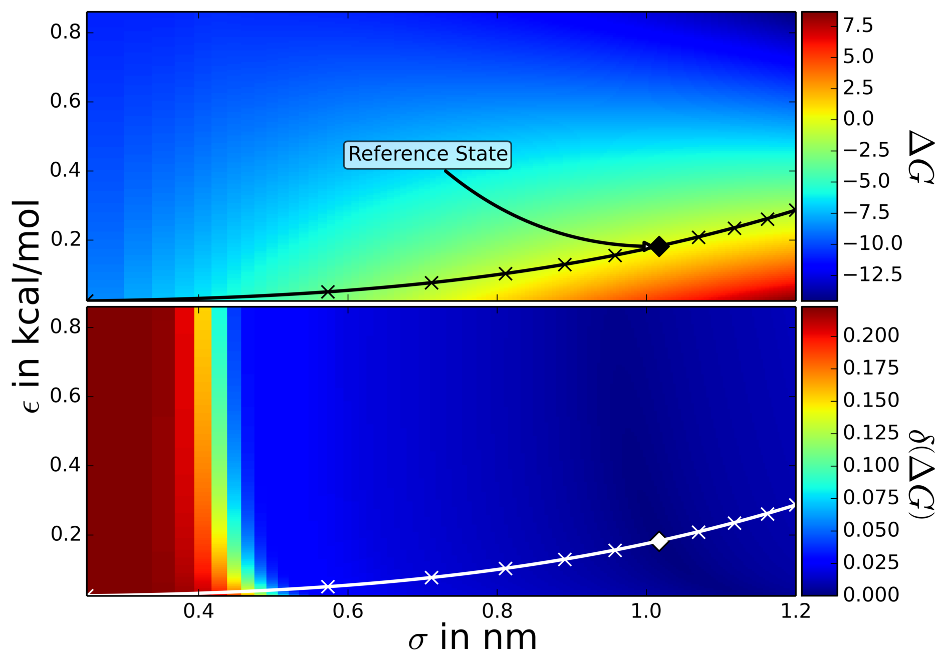
(a) Original 11 sampled states

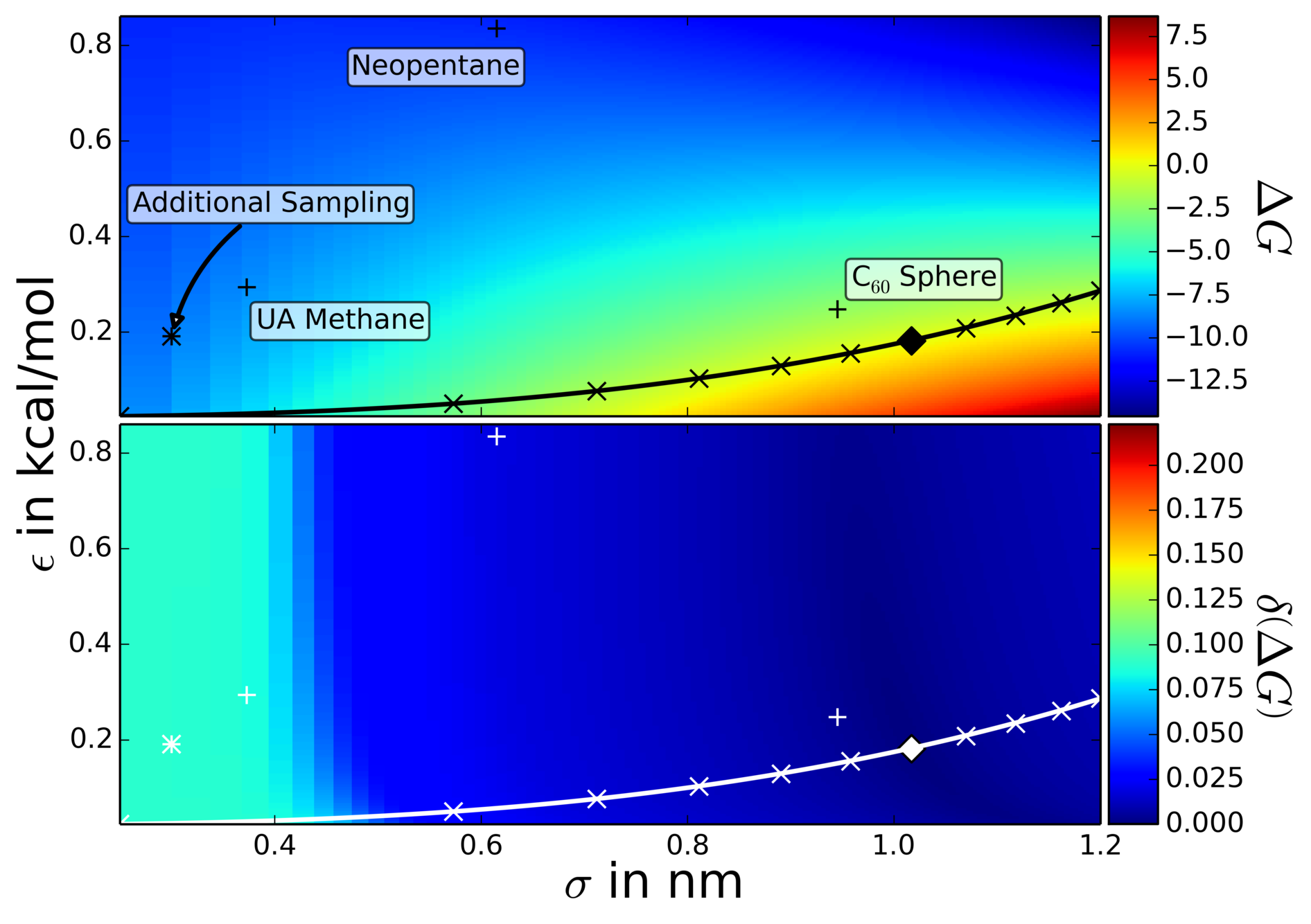
(b) Naive additional sampling at 12 states and spot checks of Lennard-Jones spheres

Figure 2: The free energies at any combination of nonbonded parameters can be predicted in post-processing and regions of large uncertainty can be quickly found. Shown is the free energy (top panels) and statistical error in the free energy (bottom panels) for $151^{2}$ parameter combinations of $\epsilon_{ii}$ and $\sigma_{ii}$ with no charge. Samples were drawn at locations shown by an X and the drawn line is to guide the eye. The free energies are all relative to the reference state shown by the diamond. LABEL:sub@fig:LJ11 shows the estimates drawing samples from 11 states only. A large region of uncertainty is seen at small $\sigma_{ii}$. LABEL:sub@fig:LJ12 A 12${}^{\text{th}}$ state was sampled in the region of high uncertainty, reducing the uncertainty in the whole region. The relative free energy of solvation was compared to chemically realistic spheres through direct simulation and is within error of the $\delta\Delta G$. Free energy is shown in units of $\text{kcal}/\text{mol}$.

For the 2D problem, regions of large uncertainty can quickly identified by visual inspection, and additional samples can drawn to reduce uncertainty. Fig. 2a shows the estimates of the solvation free energy when sampling from only 11 equivolume spaced states. We can see in the figure that parameter combinations with roughly $\sigma_{ii}<0.5\,\text{nm}$ have high estimated uncertainty with respect to the reference state. We can naively sample by a single additional state in this region which drastically reduce the error in our estimation across this range as shown in Fig. 2b. The error is a much steeper function of $\sigma_{ii}$ than $\epsilon_{ii}$ in these ranges since large particles share virtually no configuration space overlap with small particles in a dense fluid due to changes in the packing of solvent particles around small solutes.

The linear basis functions approach reproduces the results from direct fixed-parameter solvation simulations. Fig. 2b is annotated to show where several chemically realistic Lennard-Jones spheres fall in the parameter space. Solvation simulations were run for the parameters of united atom (UA) methane, ^{12, 43, 44} neopentane ⁵⁷, and a sphere roughly the size of a C₆₀ molecule. ²⁹ The relative free energies are statistically indistinguishable between the direct solvation simulations and those computed in Fig. 2b. The exact numbers and methods for the solvation simulations are shown in the supplementary material in Section S.2.

4.2 Solvation properties over a 3-D parameter space

Even visualizing the thermodynamic properties and their uncertainties in 3-D space is a nontrivial task. Iterative determination of optimal states to sample is significantly harder. Fig. 3 shows the relative solvation free energy in the 3-D parameter space for three slices of fixed $q_{i}$, and samples drawn from the initial 21 states. Because the reference state is an uncharged particle, there is large uncertainty in the relative solvation free energy to charged particles, as seen by Fig. 3a and Fig. 3c. We show the entire 3-D space of solvation free energy as a function of the three force fields parameters in animated movie provided in the supplementary material. ⁵⁵

(a)

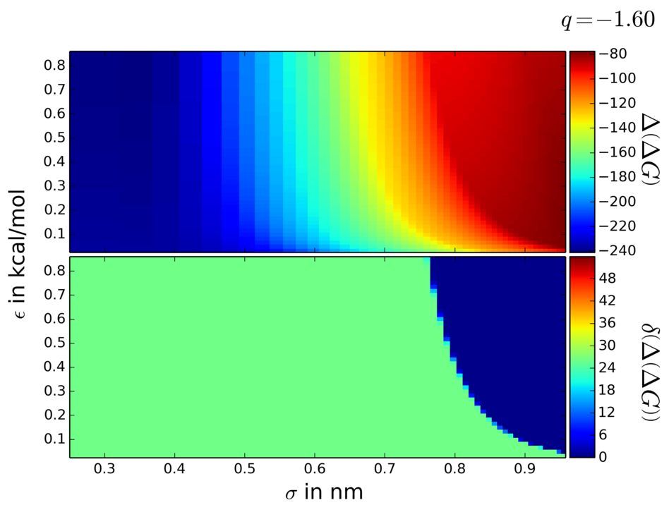
(b)

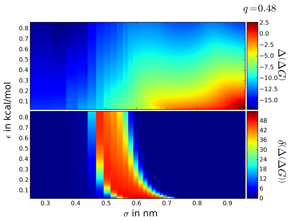
(c)

Figure 3: The free energies in a multidimensional nonbonded parameter space can be estimated and visualized rapidly. Shown are slices of the 3-D parameter space cube at fixed $q_{i}$ with the initial sampling of 21 states. Because the reference state is an uncharged particle, the error to charged parameters is large. The lack of configuration space overlap causes the uncertainty in the error estimate is large and unconverged. LABEL:sub@fig:n21-f6 and LABEL:sub@fig:n21-f31 show samples of the free energy on either side of $q=0$. LABEL:sub@fig:n21-odd shows a discontinuous jump in uncertainty between the nearby charge $q=-1.52$ in LABEL:sub@fig:n21-f6, an artifact of poor configuration space overlap. Animated movies showing the full free energy and uncertainty across the whole parameter space for initial and final samplings are included in the supplementary materials. ⁵⁵ Free energy is shown in units of $\text{kcal}/\text{mol}$.

Regions of poor configuration space overlap and large uncertainty can be visually identified in the initial simulations. Fig. 3a and Fig. 3b are taken from two nearby values of charge. One would expect the uncertainty to change smoothly with the partial charges differing by only $0.08$, however the magnitude of the uncertainty changes by a factor of nearly two, causing a visual artifact. Unless there is some sort of phase change in the system (which, as it turns out, there is not), these sorts of artifact indicates that there is little configuration space overlap, and thus both the free energies themselves as well as the estimate of the uncertainties have not converged. In order to improve our estimates, additional samples must be drawn at new parameter combinations to improve the configuration space overlap between our reference point and parameter regions such as the ones in Fig. 3b. However, deciding exactly where to put these new samples cannot be easily done by visual inspection as in the 2-D case. We must identify an algorithmic ways of placing these new points that can be easily automated, rather than having to do time-consuming manual trial-and-error.

4.3 Adaptive sampling in 3-D parameter space and improving configuration space overlap

As noted before, explicit thermodynamic paths need not be be directly defined by the user if property estimates are made by reweighting samples spanning the configuration space of all parameters of interest. A multistate statistical analysis method such as MBAR ³⁹ takes into account the configuration space overlap from all samples relative to the state of interest. The concept of a single “path” is now obsolete since any two states are now connected through a network of configuration space overlap and connected states. Sufficient configuration space overlap between all of the states of interest and sampled states results in low statistical error in estimating relative properties between states on the network.

We define two types of configurational space overlap that help us better describe the issues of searching a multidimensional parameter space. We define the local configuration space overlap as the set of configurations shared between simulations performed at an arbitrary parameter combination, and other nearby parameter combinations up to some finite $\pm p$ away in parameter space, where $p$ is one of the parameters of interest. We also define global configuration space overlap as the extent to which all points of interest in the parameter space are connected to all other points in this parameter space through a connected network of regions with local configuration space overlap.

A key issue in sampling multidimensional parameter spaces is that the most naive adaptive sampling will lead to local configuration space overlap, but not global configuration space overlap. The intuitive place to put additional samples to improve uncertainties in a free energy calculation might initially be the parameter combinations where uncertainties are the largest. Sampling only the largest uncertainty point may improve the local configuration space overlap for states near this sampled state, but does not necessarily create a network of states with global configuration space overlap connecting the reference state and the state of interest. Without a connected network, the uncertainty in relative solvation free energy differences between states inside the local neighborhood of states becomes smaller, but uncertainty to the reference state, or any other state outside of the local configuration space overlap, will still be large. The presence of local overlap but not global overlap is easy to identify when sampling along a 1-D path, since it is easy to tell where along the path there are insufficient samples. Global overlap is harder to identify and create in higher dimensional space since it is much less obvious where new samples should be placed. We need not place samples in all places where they do not occur; we instead must identify approaches that can automatically construct a network of overlapping states.

In our previous studies, ^{29, 30} optimizing the alchemical switches to identify the most statistically efficient pathways worked well to optimize alchemical paths in one dimension. Analyzing the sample variance in thermodynamic integration (TI) along paths and optimizing the $h_{n}(\lambda_{n})$ to reduced this variance identified the lowest error pathway. However, since we need a network of connected states in multidimensional space, optimizing TI would require reducing the multidimensional space to 1-D and connecting each state along a fixed path, However, since there are many possible ways to connect states in multidimensional space, optimizing TI in this multidimensional space would require connecting each state to every other state along a fixed path, resulting in $(51^{3})!$, more than $10^{10^{5}}$ possible overlapping paths, assuming the paths was restricted to visiting each state only once. We can instead create a collection of states that creates a global configuration space overlap network over the entire space by sampling discrete states in the multidimensional space, then analyzing the configuration space overlap between pairs of states with MBAR. ³⁹

We used an array of clustering and image recognition algorithms, outlined in further detail in the supporting information, to find clusters of local phase space overlap and connect them, gradually improving global configuration space overlap. Local phase space overlap was identified in the $51^{3}$ grid by identifying adjacent points having nearly identical statistical uncertainty to the reference state. When leaving these regions, the estimate of the statistical uncertainty changes discontinuously. Lack of configuration space overlap between two clusters results in a nearly constant large uncertainty estimate between any two points in either cluster. Treating the grid of uncertainty estimates to the reference state as a function of the three parameters, we interpreted this as a 3-D image. We used SciPy’s ⁵⁸ multi-dimensional image processing module, ndimage, along with a density-based clustering algorithm, DBSCAN, ⁵⁹ to identify clusters of grid points with local configuration space overlap based on estimated statistical uncertainty.

We choose a new state to sample inside each cluster of local configuration space overlap. Each cluster was treated as volume occupying shape in the parameter space, and each shape had a boundary identified as the parameter combinations on the border of the cluster. We chose one new state inside a given cluster to sample at a random location inside the cluster. We then drew a series of line connecting this new state to the reference state, and this new state to each other cluster’s new state. We identify the intersection of the series of lines with the cluster boundaries with SciPy’s Sobel boundary detection algorithm. ⁶⁰ Sampling the additional point on the boundary of the cluster provides a way to extend the area of local configuration space overlap until clusters joined to create a network of configuration space overlap, eventually creating global configuration space overlap; we detail how we choose point on the boundary below. We iteratively apply this until it creates global configuration space overlap through a network of connected states.

By using a variety of graph theory methods, we cam propose new states at local configuration space boundaries that help to minimize the number of sampled states required to get good sampling across the parameter space. We briefly summarize the algorithm here, with additional details of the algorithm covered in the supplementary material ⁵⁵ in section S.3. The implementation used is available online. ⁵⁶ We generated a complete, weighted graph where the new states identified inside each cluster were the vertices, and each edge were the lines connecting the new states between clusters and the reference state. The weight of each edge connecting the vertices was computed by numerical integration of the uncertainty at uniformly spaced points in Euclidean space on the edge. The uncertainty of each integration point was estimated by multidimensional interpolation from nearby grid points since many integration points were not on the $51^{3}$ grid. A minimum spanning tree (MST) was created from this complete weighted graph using Kruskal’s algorithm ⁶¹ implemented in SciPy’s sparse graph routines. We sampled the vertices of the MST, residing inside a high uncertainty cluster, and the intersection of the MST’s edges with the boundary of the cluster as the final set of states sampled in the next iteration of the algorithm. This approach has the advantage of scaling to arbitrary $N$-dimensions, as direct visualization of higher dimensional spaces becomes increasingly difficult.

Statistical uncertainties in the free energy differences between states are reduced by two orders of magnitude even though the amount of sampling is only increased by nine times (21 to 204 states), because this adaptive algorithm generates good global configuration space overlap. Fig. 4 shows the same three slices of the 3-D parameter space as Fig. 3, now with 203 sampled parameter combinations, all adaptively chosen except for the initial 21 combinations. We estimated properties at 101 $\sigma_{ii}$ points for the figure to improve image quality. All time comparisons are made assuming $51^{3}$ parameter combinations. During this process, the maximum error in relative solvation free energy differences was reduced from $53.405\,\text{kcal}/\text{mol}$ to $0.631\,\text{kcal}/\text{mol}$ and the mean error was reduced from $16.162\,\text{kcal}/\text{mol}$ to $0.118\,\text{kcal}/\text{mol}$. However, the initial uncertainty is a misleading underestimate as much of the parameter space had no global configuration space overlap with the reference state, meaning the error estimates are unconverged.

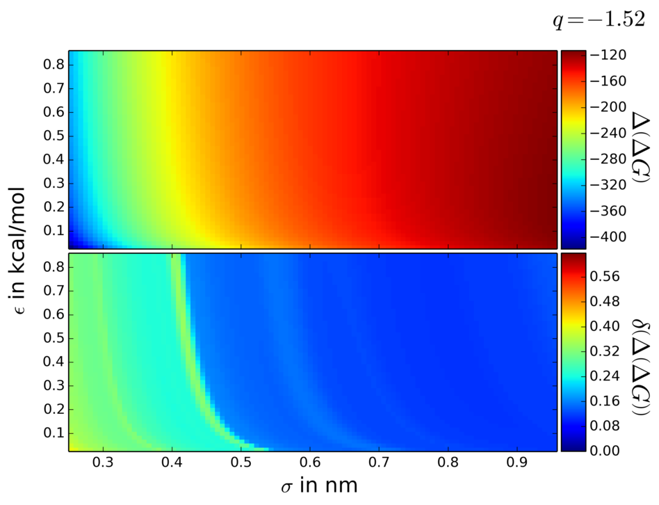
(a)

(b)

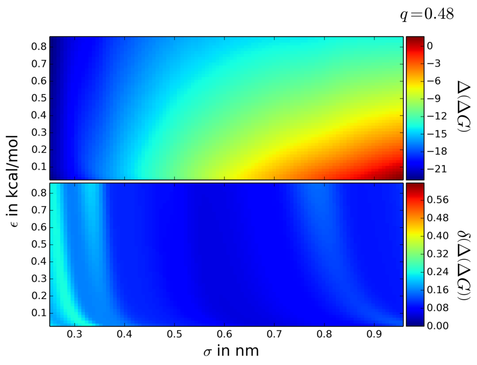
(c)

Figure 4: Adaptive sampling allows reduction of the uncertainty in the whole multidimensional nonbonded parameter space. Shown are slices of the 3-D parameter space cube at the same fixed $q_{i}$ as in Fig. 3. The total uncertainty has been reduced by more than an order of magnitude with only a few adaptive iterations and a total of 203 sampled states. LABEL:sub@fig:n203-f38 and LABEL:sub@fig:n203-f21 have significantly reduced error relative to their counterparts in Fig. 3. LABEL:sub@fig:n203-odd no longer has the discontinuous uncertainty as it did in Fig. 3. Animated movies showing the full free energy and uncertainty across the whole parameter space are included in the supplementary materials. ⁵⁵ Free energy is shown in units of $\text{kcal}/\text{mol}$.

The consequences of the poor configuration space overlap can be seen in Fig. 5 where the maximum and mean uncertainty jumps at a certain iterations. The jumps in uncertainty indicate that a new region of poor configuration space overlap has been identified and partially sampled. Ways to monitor when global configuration space overlap has been reached are discussed in Section 4.6.

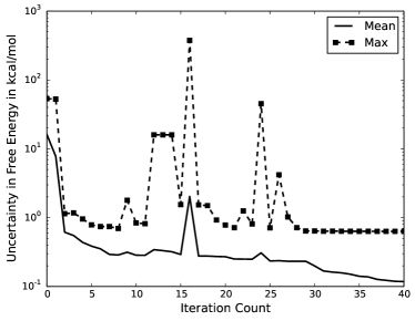
Figure 5: Discovery of regions of poor configuration space overlap appear as sudden jumps in the maximum uncertainty from between two iterations, but these regions are joined by sampling adaptively. The mean (solid) and maximum (dashed) uncertainty in the free energy for the 3-D nonbonded parameter combinations are plotted as function of iteration of the algorithm. The algorithm reduces the uncertainty of the largest areas of uncertainty before moving to others, where it can find regions of no configuration space overlap. Once some configuration space overlap is found through adaptive sampling, the uncertainty jumps as a more converged estimate can be made. The iterative process improves phase space overlap and lowers overall uncertainty. Uncertainty in free energy is shown in units of $\text{kcal}/\text{mol}$ and shown using a logarithmic scale to show changes at both large and small maximum uncertainty.

The adaptive sampling algorithm correctly places samples to reduce regions of poor configuration space overlap. Fig. 6 shows all of the sampled states in a scatter plot of the 3-D parameter space. Subsequent adaptive iterations are shown in color scale ranging from blue for the initial iterations to red in the final iteration. The large clustering of points is expected at small $\sigma_{ii}$, small $\epsilon_{ii}$, and large $q_{i}$, because the water tightly rearranges around the particle due to very large Coulombic interactions. The tightly packed water arrangements share little no configuration space overlap with any other parameter combinations, so many samples at these states and connecting states are needed to accurately estimate properties.

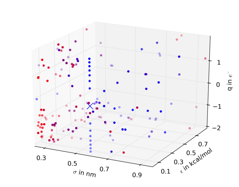
Figure 6: The adaptive sampling algorithm samples the entire parameter space. The sampled states are shown as a scatter plot with successive iterations moving from initial (blue) to final (red) as a function of the 3-D parameter space. Many new states are selected at small $\sigma_{ii}$ as large uncertainty in the region is identified from successive iterations. Fewer samples states are needed at intermediate $\sigma_{ii}$ as the configuration space overlap to states already sampled is high. The reference state is shown as an X.

The bottleneck of computing the energies is completely removed with the linear basis function approach. There are more than five times more states in the 3-D parameter (132,651) space than the 2-D space (22,801). Despite this, computational cost to compute the energies in 3-D space only increases to less than 30 CPU seconds for 21 sampled states, and just over 50 CPU seconds for 203 sampled states. Taking again the conservative average of $1500$ CPU seconds needed per rerun, computing the energies at the 132,651 parameter combinations would have taken over 132 and 1280 CPU years for 21 and 203 sampled states, respectively. Optimized code to explicitly calculate the basis functions at the time of the force calculation would allow even faster vectorized calculations than the post-processing used here, allowing this method to scale to even larger multidimensional spaces. After removing this bottleneck, the main cost is in performing the 203 simulations at sampled states and running MBAR. Our simulations took an average of 25 CPU hours per simulation to run, and MBAR calculations took 108 CPU hours to compute properties. We would need to invest the time to run simulations and compute properties with MBAR, independent of how the energies were computed.

The algorithm could be further optimized depending on the relative cost of the simulations and of MBAR over very large numbers of states. In this case, simulations were relatively cheap compared to MBAR. If the simulations were more expensive, then shorter simulations could be run between iterations. Additionally, more proposed states for direct simulation could be generated at each step to reduce wall time. For example, instead of 10 new states run for 10 ns, 20 new states could be run for 5 ns each. In general, shorter cycles of simulation plus analysis are expected to improve performance as within well-sampled regions, the error in free energy estimates scales approximately as $N^{-1/2}$. Adding significant configuration space overlap between regions that are not connected will scale significantly better.

4.4 Computing Other Thermodynamic Properties and Comparing to Reported Results

Estimating properties over the entire multidimensional parameter space at once can provide thermodynamic information which would otherwise require extensive simulations to compute at each thermodynamic state. This section looks at estimating five properties where significant simulation is required when sampling each state individually: the relative solvation entropy and enthalpy, the absolute solvation free energy of ions, the radial distribution function (RDF) focusing on the first hydration shell, and the difference between the Born solvation free energy and the simulation estimate in the free energy of charging a particle. In this section, we show how we can compute the enthalpy and entropy from the same collected data as used for free energies, compare ion parameter free energies to show accuracy and limitations in our approach, estimate RDFs without generating trajectories at the target parameters, and identify trends in the deviation of solvation free energies from the Born solvation approximation.

4.4.1 Relative Solvation Entropy and Enthalpy

We can estimate the relative solvation entropy and enthalpy alongside the relative solvation free energy without additional sampling. The relative solvation enthalpy is the difference in solvation enthalpy, $\Delta H_{\text{solv}}$, between the reference state $X$ and any other state $j$ in the multidimensional parameter space. We compute the relative enthalpy difference, $\Delta\left(\Delta H_{Xj}\right)$, as

$$\Delta\left(\Delta H_{Xj}\right)=\left\langle\Delta U_{Xj}\right\rangle\text{.}$$ (7)

Similarly the relative solvation entropy, $T\Delta\left(\Delta S_{Xj}\right)$, is computed as

$$-T\Delta\left(\Delta S_{Xj}\right)=\Delta\left(\Delta G_{Xj}\right)-\Delta\left(\Delta H_{Xj}\right)$$ (8)

where $\Delta\left(\Delta G_{Xj}\right)$ is the relative free energy of solvation, and $\left\langle\cdot\right\rangle$ is the statistical expectation value, computed here by MBAR. ³⁹ In all cases, we report the difference in thermodynamic properties with respect to the reference state. These properties we estimate have such large uncertainty from only the initial 21 states due to poor sampling that any number is essentially meaningless. Computing relative enthalpies and entropies generally requires significantly more samples to compute than relative free energies, ^{38, 62, 63} as only samples with local phase space overlap to the end states contribute to precision of expectations of observables such as the enthalpy.

Additional sampling reduces the uncertainty in the estimates of relative solvation entropy and enthalpy by orders of magnitude, but not to the same extent as the uncertainty in the free energy. This is because whether or not there is good global phase space overlap does not ensure that a given state has good local phase space overlap with its neighbors. Fig. 7 shows the relative solvation entropy and enthalpy estimations, along with uncertainty at 203 sampled states. The uncertainty smoothly transitions between adjacent states, suggesting the estimates are numerically converged. However, the maximum uncertainty is several orders of magnitude larger than the relative solvation free energy. The maximum uncertainty in relative solvation entropy changes from an uncertain estimate to $0.193\,\text{kcal}/\left(\text{mol}\cdot K\right)$, and the relative solvation enthalpy’s maximum uncertainty drops to $57.5\,\text{kcal}/\text{mol}$. The mean uncertainty for relative solvation entropy and enthalpy fall to $0.0147\,\text{kcal}/\left(\text{mol}\cdot K\right)$ and $4.37\,\text{kcal}/\text{mol}$, respectively. Although these error estimates are still too large to make practical predictions of solvation entropies, the estimates of the errors from the 203 states are well-defined, which is a marked improvement over the initial sampled states. The whole configuration space has been sampled, and all states now have at least moderate local phase space overlap with its neighbors. Once decent estimates of properties are found, we can run additional simulations on states that have the most desirable preliminary estimates of properties.

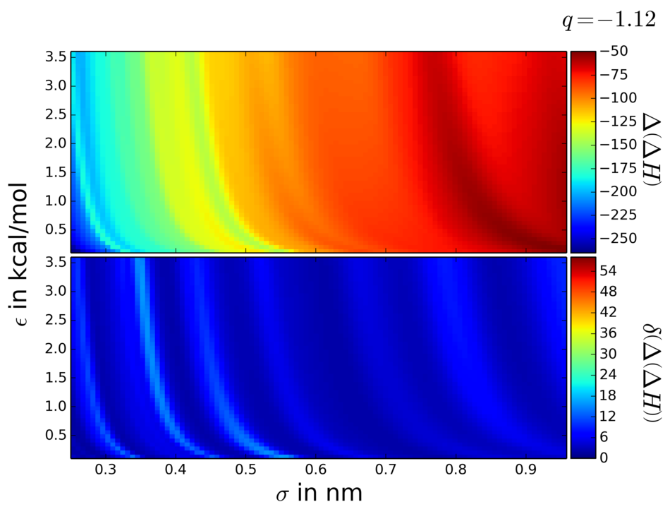
(a)

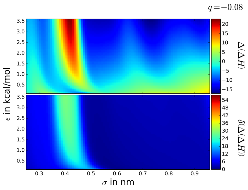
(b)

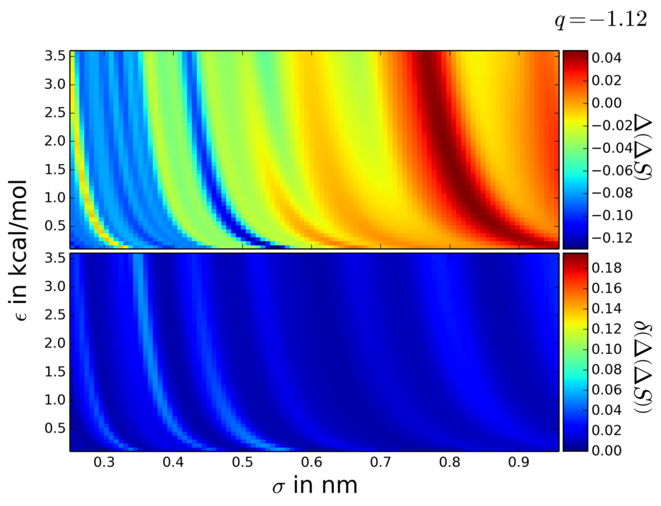
(c)

(d)

Figure 7: Uncertainty in entropy and enthalpy are also reduced with the uncertainty in the free energy. The enthalpy $H$, (LABEL:sub@fig:Hn203-f11 and LABEL:sub@fig:Hn203-f24) and entropy $S$, (LABEL:sub@fig:Sn203-f11 and LABEL:sub@fig:Sn203-f24) are computed from 203 total sampled states and reported in kcal/mol. The uncertainty in both properties now smoothly transitions between adjacent states. The uncertainty is still significantly larger than that of the free energy, which is expected as these properties require more sampling to compute accurately than the free energy. Additional samples or other means of computing these properties would be required to reduce error further.

4.4.2 Ion Solvation Free Energies

We compare the results from our study to a detailed ion parameter study by Joung and Cheatham. ⁶⁴ Their study parameterized Li⁺, Na⁺, K⁺, Rb⁺, Cs⁺, F^-, Cl^-, Br^-, and I^- in several water models including TIP3P and compared them to experimental and computational studies from others. They parameterized the ions based on several experimental observables, including free energy of solvation. We compared their absolute solvation free energies to absolute solvation free energies we computed from our method in Table 1. The table shows the ion parameters, free energy of solvation, $\Delta G$, and first hydration shell (FHS) location estimated from their work and our approach. We compute absolute solvation free energies for our work by adding the free energies from the relative simulation to those of a single set of solvation simulations of the reference particle along a soft core potential ^{46, 47} and a 1-1-6 parameterization. ^{27, 29} These simulations were run with the same conditions as described in section 3 at 11 states uniformly distributed along $\lambda$ from 0 to 1 of the soft core path.

We re-computed parameter values and adjusted the reported free energies to make the values from Joung and Cheatham ⁶⁴ comparable to this work. Their ion $\sigma_{ii}$ was calculated for Lorentz-Berthelot mixing rules. We back calculated the $\sigma_{ii}$ for geometric mixing rules in Table 1 by setting the $\sigma_{ij}$ between the ion and the oxygen in water equal in both mixing rules, giving the relation

$$\sigma_{\text{ion-ion, geo}}=\frac{\left(\sigma_{\text{ion-ion, LB}}+\sigma_{\text{OW-OW}}\right)^{2}}{4\sigma_{\text{OW-OW}}}$$ (9)

where $\sigma_{\text{ion-ion, geo}}$ is the reported ion $\sigma_{ii}$ in Table 1, $\sigma_{\text{ion-ion, LB}}$ is $\sigma_{ii}$ for the Lorentz-Berthelot mixing rule reported by Joung and Cheatham, and $\sigma_{\text{OW-OW}}$ is the TIP3P oxygen-oxygen $\sigma_{jj}$ which we assumed was constant between the mixing rules. The solvation free energies from Joung and Cheatham have been adjusted by -1.9 $\text{kcal}/\text{mol}$ to remove the correction they added for ideal gas expansion when comparing simulations, carried out with gas-phase standard states at 1 M, to experimental results, where gas-phase standard states are typically 1 atm. ^{64, 65}

Table 1: Absolute solvation free energies and first hydration shell (FHS) locations compared from this work and from Joung and Cheatham. ⁶⁴ Ion $\sigma_{ij}$ were back calculated from Lorentz-Berthelot to geometric mixing rules for ion/oxygen interactions. $\epsilon_{ii}$ and $\Delta G$ are in $\text{kcal}/\text{mol}$; $\sigma_{ii}$ and FHS location are in nm. Error in this work’s FHS computed by 200 bootstrap samples ⁶⁶ with a discretization of $\pm 0.0075$ nm.

Ion	$\sigma_{ii}$	$\epsilon_{ii}$	$\Delta G$		FHS
			Joung and Cheatham	This Work	Joung and Cheatham	This Work
Li+	0.1965	0.0290	-115.6	-105.26 $\pm$ 0.54	0.196	0.211 $\pm$ 0.016
Na+	0.2479	0.0874	-90.6	-90.63 $\pm$ 0.44	0.238	0.234 $\pm$ 0.015
K+	0.3039	0.1937	-72.6	-72.42 $\pm$ 0.36	0.275	0.279 $\pm$ 0.016
Rb+	0.3231	0.3278	-67.6	-67.31 $\pm$ 0.35	0.292	0.294 $\pm$ 0.030
Cs+	0.3532	0.4065	-62.5	-62.13 $\pm$ 0.35	0.311	0.309 $\pm$ 0.021
F-	0.4176	0.003364	-121.6	-120.91 $\pm$ 0.45	0.263	0.257 $\pm$ 0.016
Cl-	0.4617	0.0356	-91.5	-90.99 $\pm$ 0.36	0.313	0.309 $\pm$ 0.028
Br-	0.4825	0.0587	-84.8	-84.48 $\pm$ 0.36	0.329	0.333 $\pm$ 0.015
I-	0.5396	0.0537	-75.9	-75.89 $\pm$ 0.34	0.351	0.347 $\pm$ 0.017

The solvation free energies from our work and Joung and Cheatham’s work are within statistical error. The free energies from this study appearing in Table 1 are within two standard deviations of Joung and Cheatham ⁶⁴ for all ions except Li⁺, which is outside the parameter range studied. The comparable accuracy of our results to those of Joung and Cheatham provide validation for the free energies we report. Our method has the added benefit of computing the solvation free energy for arbitrary parameter combinations. The ability to compute properties for arbitrary parameter combinations comes from sampling only 203 states plus 11 for the absolute solvation free energies. Joung and Cheatham carried out 12-13 simulations for each of the 9 ions, resulting in 108-117 simulations for comparison. We were able to compute properties at roughly 14,000 times the number of parameter combinations, for only double the simulation cost.

Our method breaks down if the parameter combination falls outside the defined range. The parameters for the Li⁺ ion in Table 1 fall significantly outside the range we searched, namely, the $\sigma_{ii}$ is less than the 0.25 nm minimum. The estimated free energy for this parameter combination is not within statistical error for that of Joung and Cheatham. ⁶⁴ The estimated value for any thermodynamic property at this ion will likely inaccurate as the estimation is now an extrapolation instead of a thermodynamically-consistent interpolation between sampled states. Estimates on parameter combinations falling just outside the searched range, such as the Na⁺ ion, appear to still be accurate, so the range of convergence of these calculations outside of samples parameters is not zero.

4.4.3 Estimating Radial Distribution Functions

We can estimate the radial distribution function (RDF or $g(r)$) of a specified parameter combination without explicitly sampling that combination. The first hydration shell and the water RDF are properties that many have tried to compute accurately and compare to experiment. ^{64, 67, 68, 69, 70, 71, 72, 73, 74} Traditionally, a RDF is generated by measuring the distances between two specified atomic groups (e.g. ion-water, water oxygen-water oxygen, etc.) generated over a trajectory, counting the number of pairs that are within a shell of size $r+\delta r$, then average over the shell volume and whole trajectory. The fact that the RDF is an average property and dependent only on the configuration implies it is a thermodynamic equilibrium property which can be computed as a statistical observable. Computing an equilibrium expectation value of some observable, A, with MBAR ³⁹ is

$$\left\langle A\right\rangle_{a}=\sum_{n=1}^{N}W_{na}A(\mathbf{x}_{n})$$ (10)

where the summation runs over all samples in all states, $W_{na}$ are the statistical weights from reweighting each $n$th drawn sample in the $a$th state, the $A(\mathbf{x}_{n})$ are the observed values from sample $n$ and are functions of the configuration, $\mathbf{x}$. The weight MBAR assigns to each sample $n$ is ³⁹:

$$W_{na}=\frac{e^{f_{a}-u_{a}(\mathbf{x}_{n})}}{\sum_{k=1}^{K}N_{k}e^{f_{k}-u_{k}(\mathbf{x}_{n})}}$$ (11)

where $f_{a}$ is the reduced free energy ($\beta A$ or $\beta G$) of state $a$, $u_{a}(\mathbf{x}_{n})$ is the reduced internal energy ($\beta U$) of the configuration $\mathbf{x}_{n}$ in state $a$, and $N_{k}$ is the number of samples collected from state $k$. The observable for computing the RDF is the discrete count of pairs within a specified $r+\delta r$ shell normalized by the shell radius and the number volume $\rho=N_{\text{particles}}/V$. We must estimate the RDF at multiple shell volumes in order to generate a complete RDF curve.

The first hydration shells (FHS) are accurately predicted by the RDF estimation. Fig. 8 shows the RDF estimated for the Li⁺ and the Cl^- ions from Joung and Cheatham. ⁶⁴ The RDF is estimated at 160 discrete bins (0.0075 nm spacing) from $r=0$ to $r=1.2$ nm along with the error in that estimate. The black curves in Fig. 8 are the estimates from MBAR computed purely from data collected at our 203 states, and not from any data drawn at the ion’s parameters. Error in the MBAR estimate is shown as dashed lines and is two standard deviations of the uncertainty in the RDF, also computed by MBAR. To validate the MBAR results, the green curves in Fig. 8 show the RDF computed from simulations at the given ion’s parameters. The data from these direct simulations of the ions were not used in the MBAR estimate. The error in the green curves is taken from 200 bootstrap samples ⁶⁶ of the RDF for each ion. The Li⁺ ion RDF is shown in Fig. 8b to again emphasize that estimates made outside the parameter range tend to break down, evidenced by the erratic behavior in the RDF.

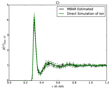
(a) Cl^-

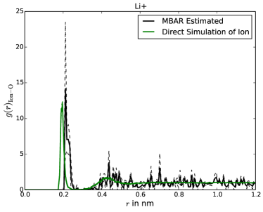
(b) Li⁺

Figure 8: Radial distribution functions (RDF) can be estimated at any parameter combination inside the parameter search range. The ion-oxygen RDF in TIP3P water is shown for Cl^- and Li⁺ with Joung and Cheatham parameters. ⁶⁴ The RDFs are estimated without sampling the explicit parameter combinations using 160 discrete bins. Estimates made from parameters inside the parameter range, Cl^- LABEL:sub@fig:rdf-Cl are accurate as the first hydration shell is predicted within error to Joung and Cheatham. ⁶⁴ in Table 1. Estimating parameters which fall outside the searched parameter range, Li⁺ LABEL:sub@fig:rdf-Li, are inaccurate. Error is shown dashed lines of two standard deviations, computed by MBAR for the black curves and 200 bootstrap samples for the green curves.

The Cl^- ion in Fig. 8a shows an example where we can estimate solvation structure and improve future simulations. We further validated the RDF calculation by determining the peak of the first hydration shell for every ion from Joung and Cheatham as the bin with highest occupancy ⁶⁴ and compared our results to theirs in Table 1. The peaks we estimate and those from Joung and Cheatham are in agreement with each other, within the error of our bin width of 0.0075 nm. The RDF curves generated using reweighting are not as smooth as the RDF curves from other studies, and we do not expect them to be smooth with the range of parameters we searched. However, all features are well preserved. This approach can be used to broadly search parameter space and generate approximate RDF’s, until those that replicates the RDF or hydration shell properties of interest are identified. Further simulations could then be run around the sets of properties which gave the RDF replicating the target properties to make more accurate estimates, resulting in searches over a much narrower parameter space than examined through here. A complete set of the RDFs estimated via reweighting and direct simulation for every ion is included in the supplementary material. ⁵⁵

4.4.4 Born Approximation to Solvation Free Energy

The Born approximation to solvation free energy measures the effort to transfer a charged particle between two dielectrics. The free energy differences for this approximation of transferring a hard sphere particle between vacuum and a fluid is

$$\Delta G=\frac{q^{2}}{4\pi\epsilon_{0}R_{ij}}\left(\frac{1}{\epsilon_{d}}-1\right)$$ (12)

where $\epsilon_{d}=92$ is the estimated dielectric constant of our fluid, TIP3P water ⁷⁵, and $R_{ij}$ is the Born radius.

We can estimate the Born radius of any particle in our search space from our sampled states. Choosing the correct Born radius, or effective hard sphere (EHS) radius is a nontrivial task. However, we can estimate the EHS radius with our RDF calculation. We first compute the RDF for a given parameter combination, $g(r)$, then compute the EHS radius by determining an $r_{0}$ where the following conditions for the oxygen-ion g(r) are met:

$$g(r_{0}-\delta r) =0$$ (13)

$$g(r_{0}) =0$$ (14)

$$g(r_{0}+\delta r) >0$$ (15)

to a tolerance of $10^{-5}$. $r_{0}$ can be interpreted as the point on $g(r)$ where the probability of finding a particle changes from zero to nonzero. We set $R_{ij}=r_{0}$ for the Born solvation calculations.

We applied correction terms to our estimated free energies to remove errors introduced by our choice of simulation settings and water model. These corrections allow a comparison of free energy between different methods without having a methodological dependence. All of the corrections we applied are detailed in Hünenberger and Reif ⁷⁶ and we go through explicit detail of which corrections we applied and why in the supplementary material ⁵⁵ in section S.6.

There are a number of reasons the the Born approximation is not perfect for our particle-water system. These imperfections come from not simulating a truly infinite medium, the water model having an asymmetric charge distribution, Lennard-Jones terms affecting the free energy of transfer, and the fact that $R_{ij}$ may change on charging since we have soft particles. We are interested in identifying deviations from the Born approximation with our method, given that we fully expect deviations from these imperfections.

The Born approximation to the solvation free energy is the free energy of transferring a charged hard sphere with radius $R_{ij}$, not for the free energy of solvating the uncharged particle. To remove this dependence on the cavitation free energy, ⁷⁶ we we estimate the $R_{ij}$ from the RDF as described above for each uncharged combination of $\sigma_{ij}$ and $\epsilon_{ij}$, then calculate the free energy difference to the same values of $\sigma_{ij}$ and $\epsilon_{ij}$ but with a charge. This allows us to compare our free energy of charging to the Born approximation to the free energy of charging, and identify deviations between the model and our simulation. We do not recalculate $R_{ij}$ at the end state.

Both trends and failures of the Born approximation can be easily visualized for the entire parameter space. Fig. 9 shows the difference between the Born approximation ($\Delta G_{\text{Born}}$) and this work’s estimate for the charging free energy ($\Delta G_{\text{TW}}$). Any deviation from $\Delta\Delta G_{\text{TW-Born}}=0$ indicates nonidealities relative to Born approximation to the free energy of charging. There are several deviations which can be seen in the figure. The first deviation is the Born free energy generally predicts less favorable solvation free energy for both signs on the charged particles ($\Delta G_{\text{TW}}<\Delta G_{\text{Born}}<0$). However, this deviation is asymmetric as the deviation in from Born theory of the positively charged particle at $q=+2$ is up to $-152.1\,\text{kcal}/\text{mol}$, but the negatively charged particle only deviates up to $-78.5\,\text{kcal}/\text{mol}$ at $q=-2$. The charging free energy more strongly depends on $\sigma_{ii}$ for the positive particle as the $\Delta\left(\Delta G\right)$ in Fig. 9a spans 13.7 $\text{kcal}/\text{mol}$ from $\sigma_{ii}\approx 0.5$ to $\sigma_{ii}\approx 0.95$ on average, whereas in Fig. 9b the span 27.6 $\text{kcal}/\text{mol}$ on average in the same range of $\sigma_{ii}$. We can also observe the opposite case where the Born estimate is more favorable than the observed estimate ($\Delta G_{\text{Born}}<\Delta G_{\text{TW}}<0$) in Fig. 9a where $\Delta\left(\Delta G\right)>0$ at small $\sigma_{ii}$ and $\epsilon_{ii}$. This opposite case occurs because the negatively charged particle attracts the water’s hydrogens, which do not have Lennard-Jones interactions, and would be able to approach much more closely than the Born model predicts with its hard sphere approximation. Simply estimating free energy at a few states in the parameter space would have been insufficient to observe these broad trends as a significant degree of interpolation, or worse extrapolation, would have been required.

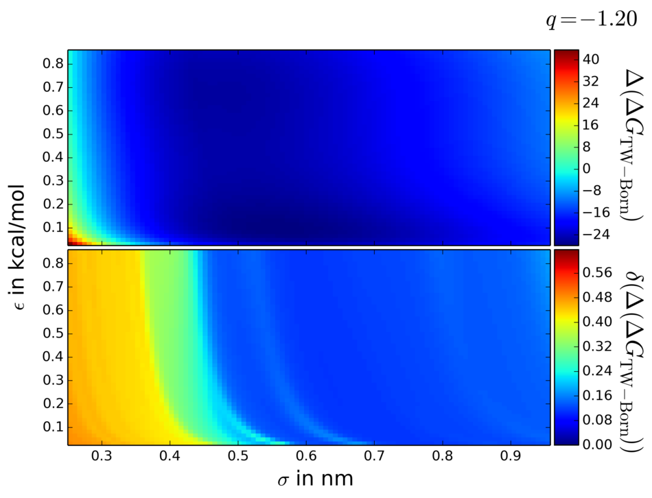
(a)

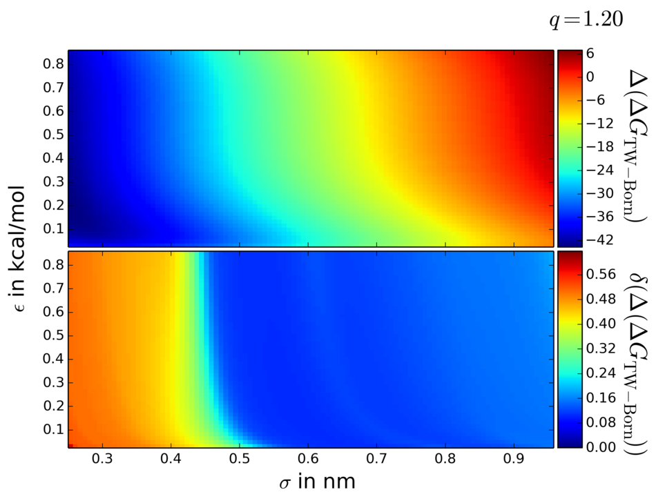
(b)

Figure 9: Trends and failures in approximations can be visualized over wide parameter space. The deviation of the Born hydration free energy from the computed solvation free energy is shown for two fixed slices of $q_{i}$. Explicitly shown is the Born free energy minus this work’s free energy estimates: $\Delta G_{\text{Born}}-\Delta G_{\text{TW}}$. Free energy difference estimates for each combination of $\sigma_{ii}$ and $\epsilon_{ij}$ are relative to the same combination at $q_{i}=0$ as to approximate only the contribution of charging a given sphere in solvent. LABEL:sub@fig:B203-f10 and LABEL:sub@fig:B203-f40 show the deviations with the solute carrying a $\pm q$ charge. The Born model generally predicts a more favorable interaction relative to the simulation. An exception to this trend is at very small $\sigma_{ii}$ and $\epsilon_{ii}$ for a negatively charged particle where it predicts a less favorable interaction than the simulation as the TIP3P water hydrogens can tightly pack around the particle. Animated movies showing the full free energy and uncertainty across the whole parameter space are included in the supplementary materials. ⁵⁵ Free energy is shown in units of $\text{kcal}/\text{mol}$.

A full animation showing $\Delta\Delta G_{\text{TW-Born}}$ at combination in the parameter space is included in the supplementary material. ⁵⁵

4.5 Monitoring numerical bias

The numerical bias caused by the process of calculating energies from perturbations of reference states can be minimized. Eq. (6) and in the supplementary material Eq. S.5 involve the addition and subtraction of many small numbers, depending on reference states $X$ and $Y$. This can lead to rounding errors which may propagate to the simulation package and be made worse by the software’s precision. Choosing reference states with larger $\Delta C_{n,XY}$ can help reduce accumulation of error. If the software natively allows access to the basis function values, then this source of numerical error is eliminated. However, we must quantify our numerical error here since the perturbation approach was chosen.

We find that rounding errors do not propagate from the perturbed basis function representation to the thermodynamic properties for these calculations. The rounding errors for this system were checked by evaluating the energy of each sampled configuration at every sampled state as though we did not use the basis function approach. The energies of every configuration evaluated at every sampled state computed from directly from GROMACS were compared to the energies computed from the basis functions and any deviation was a result of numerical bias. The energies computed from basis function calculations and the energies directly from GROMACS reruns differed by less than $0.002\%$. This very small relative error does not assure that errors themselves are negligible, since large energies have large absolute errors. The largest absolute error in all 203 simulations was was $11.804\,\text{kcal}/\text{mol}$, which at first appears is likely to have a significant effect in the final answers. However, these large absolute errors do not affect any of the property estimates. This is because these large rounding errors occur when the trajectory from a particle with small $\sigma_{ii}$ is evaluated in a force field for a particle with large $\sigma_{ii}$. This often resulted in the oxygen of TIP3P water being within the large particle’s excluded volume, resulting in a highly repulsive interaction. Every configuration with rounding error in this study had a Boltzmann weight, $\exp\left(-\beta U(r,\lambda)\right)$, indistinguishable from zero at machine precision, and thus these errors do not contribute to any of the properties of interest. The energies calculated using reference states thus give results that are sufficiently close to those from direct evaluation of the energies for all uses.

4.6 Convergence and alternate algorithm conditions

Examining the uncertainty estimate from the reference state alone is insufficient to determine convergence of the calculations. The multidimensional space initially has many regions of configuration space overlap, which causes unconverged estimates of the properties and their uncertainties. Poor overlap implies that the mean and the maximum uncertainty alone are not appropriate gauges for convergence since the error does not consistently decrease with number of samples as observed in Fig. 5. As discussed above, a network of overlapping configuration space between all states required for accurate estimate of properties and quantification of the uncertainties in these properties, and we need a way to diagnose whether this network has been created at a given stage of the simulation.

The configuration space overlap can be analyzed through a multidimensional extension of the Overlapping Distribution Method. ^{19, 77} This method can quantify the overlap between states by considering the probability of each sample occurring in every state. The unnormalized probability of a sample can be computed from its Boltzmann weight. Just as each sampled configuration carries a Boltzmann weight for the state in which it was drawn, the configurations can be reweighted to all other states to determine what the relative Boltzmann weights are in the other sampled states. ^{35, 40, 41, 39, 78} MBAR ³⁹ stores each sample’s weights as a matrix $\mathbf{W}$, the same matrix of weights discussed earlier in the context of expectations whose entries are $W_{na}$. The pairwise probabilities can be assembled in what we term the “overlap matrix,” constructed from the matrix of weights. This multidimensional overlap matrix is calculated from the weights as

$$\mathbf{O}=\mathbf{W}^{\mathbf{T}}\mathbf{W}\mathbf{N}$$ (16)

where $\mathbf{N}$ is a diagonal matrix with each $i$th entry equal to the number of samples from the $i$th state. ^{79, 39} The individual elements of the overlap matrix, $O_{ij}$, can be read as the probability of a sample generated in state $j$ being observed in state $i$. Since $\mathbf{O}$ is a Markov matrix, it can be shown that $\mathbf{O}$ will have at least one eigenvalue of $1$, which is also the maximum over all eigenvalues. All other eigenvalues will be real and positive. ⁷⁹ However, multiple eigenvalues of $1$ in $\mathbf{O}$ indicate that there are discontinuous regions of sampled configuration space and $\mathbf{O}$ can be rearranged to a block diagonal matrix that illustrates which states are and are not connected. Thermodynamic property measurements made between the discontinuous configuration spaces will have undefined uncertainty, which numerically can show up as either NaN or very large numbers that change dramatically with small changes in sampling. ⁷⁹

Monitoring both the eigenvalues of the overlap matrix and maximum uncertainty can provide good guidance as to when converged property estimates have been reached. Monitoring exclusively the eigenvalues of $\mathbf{O}$ is insufficient to determine convergence over the entire parameter space since $\mathbf{O}$ only involves the sampled states. However, if the sampled states are well-enough dispersed such that the estimated uncertainties of all the unsampled states are low, and simultaneously all the sampled states are connected as demonstrated by having a single eigenvalue with value 1 for $\mathbf{O}$, we can have high confidence that the uncertainty estimates are reliable.

We therefore defined our property estimates as converged once there were no repeated eigenvalues of $1$ in $\mathbf{O}$, and once no further clusters of uncertainties in the relative free energy above the target threshold are found, i.e. the clustering algorithm can not find new points adjacent grid points with large uncertainty. If desired, the uncertainty can be iteratively reduced by lowering the error threshold of the algorithm. The deviation of the five largest eigenvalues from 1 are shown for each iteration in the supplementary material in Table S.2.

The proposed adaptive sampling algorithm is only an initial proposal, and sampling regions of poor configuration space overlap could be improved by changes to this algorithm. For example, the algorithm discussed here and detailed in the supplementary information ⁵⁵ identified clusters of high relative uncertainty by counting the number of grid points in the cluster. This resulted in many states being chosen adaptive at larger $\sigma_{ii}$ due to the density of grid points, despite the fact that most of the regions with no phase space overlap were at $\sigma_{ii}<0.35\,\text{nm}$. Although states were eventually placed at small $\sigma_{ii}$, one improvement could be to place points in regions with the largest integrated uncertainty, using the uncertainty as a weighting on the overall number of grid points. This improvement would still favor the larger clusters, but to a lesser extent as new pockets of poor configuration space overlap are identified and the uncertainty jumps back up as in Fig. 5.

The current study was used to determine high accuracy free energies over entire large parameter range, and this study’s range of nonbonded parameters will likely exceed many practical applications. However, this parameter search method could be adaptively shrunk to hone in on specific property estimates. Instead of determining the thermodynamic properties for a large set of starting parameters, a desired thermodynamic property could be provided and a set of parameters which generate this property are searched for, as is the case for reverse property prediction. In this case, the initial grid spacing could be larger, and a rough estimate of the property surface can be acquired, spending less simulation time per iteration. Each subsequent iteration would then narrow the search area and reduce the grid spacing, seeking the target value. States from previous iterations outside the narrowed search space, can still be included in the analysis using, preventing discarded information. Alternatively, computational time can be saved by excluding these outlier states if analysis of $\mathbf{O}$ shows that these states are not actually connected to the states ultimately of interest.

Thermodynamic property estimates are not limited to relative solvation free energies, entropies, and enthalpies. Once the simulations are converged, further thermodynamic properties can be derived from derivatives and fluctuations with respect to $V$, $P$, and $T$, ^{80, 81, 82} as well as any other property computed from statistical expectation values. ³⁹

5 Conclusion

We have shown how one can rapidly estimate thermodynamic properties in a multidimensional nonbonded parameter space by combining two time saving advantages. Computing the energies required for estimating thermodynamic properties can be accelerated with linear combinations of basis functions instead of re-running simulation force loops. Estimating the thermodynamic properties in the multidimensional parameter space is possible with the binless, multidimensional, path-free statistical method, MBAR. With these methods, properties are estimated at all states of interest simultaneously without the need define how any state is connected to any others beforehand.

Converged results can be acquired by adaptively sampling the multidimensional parameter space, creating a network of globally-connected configuration space overlap between all states. Simply adding samples in regions of large uncertainty does not necessarily create configuration space overlap to all states, as the uncertainty of differences to other states is not reduced. Regions of poor configuration space overlap can be identified by examining the overlap matrix between all sampled states, and the maximum uncertainty in the unsampled states. The parameter space is then adaptively sampled until configuration space overlap is created between the reference state and all other states of interest, and uncertainties are pushed sufficiently low for the purpose at hand.

The methods shown here can help speed up future thermodynamic property searches in multidimensional parameter space. So long as the energy functions can be computed with vector operations, and do not require re-running the simulation force loops, these methods can scale to even higher dimensionality and extend to other thermodynamic properties. Re-writing the simulation code to directly provide the required basis functions would allow even faster energy evaluation, potentially removing the need to ever compute the energy of a configuration more than once.

6 Acknowledgments

The authors would like to thank Kyle Beauchamp and John Chodera at Memorial Sloan-Kettering Cancer Center for feedback and assistance in running optimized MBAR code. The authors also acknowledge the support of NSF grant CHE-1152786.

References

- Wang et al. 2014 Wang, C. C.; Pilania, G.; Boggs, S. A.; Kumar, S.; Breneman, C.; Ramprasad, R. Polymer 2014, 55, 979–988
- Harini et al. 2013 Harini, M.; Adhikari, J.; Rani, K. Y. Ind. Eng. Chem. Res. 2013, 52, 6869–6893
- Baron 2012 Baron, R., Ed. Computational Drug Discovery and Design; Humana Press: New York, 2012; p 628
- Li et al. 2012 Li, H.; Zheng, M.; Luo, X.; Zhu, W.; Jiang, H. Chem. Biol.; John Wiley & Sons, Inc., 2012; pp 23–40
- Hansen and van Gunsteren 2014 Hansen, N.; van Gunsteren, W. F. J. Chem. Theory Comput. 2014, 2632–2647
- Yang et al. 2013 Yang, Q.; Liu, D.; Zhong, C.; Li, J.-r. Chem. Rev. 2013, 113, 8261–8323
- Monticelli and Tieleman 2013 Monticelli, L.; Tieleman, D. In Biomol. Simulations SE - 8; Monticelli, L., Salonen, E., Eds.; Methods in Molecular Biology; Humana Press, 2013; Vol. 924; pp 197–213
- Mackerell et al. 1998 Mackerell, A. D.; Bashford, D.; Bellott, M.; Dunbrack, R. L.; Evanseck, J. D.; Field, M. J.; Fischer, S.; Gao, J.; Guo, H.; Ha, S.; Kuchnir, L.; Kuczera, K.; Lau, F. T. K.; Mattos, C.; Michnick, S.; Ngo, T.; Nguyen, D. T.; Prodhom, B.; Reiher, W. E.; Roux, B.; Schlenkrich, M.; Smith, J. C.; Stote, R.; Straub, J.; Watanabe, M.; Wio, J.; Yin, D.; Karplus, M. J. Phys. Chem. B 1998, 5647, 3586–3616
- Vanommeslaeghe et al. 2011 Vanommeslaeghe, K.; Hatcher, E.; Acharya, C.; Kundu, S.; Zhong, S.; Shim, J.; Darian, E.; Guvench, O.; Lopes, P.; Vorobyov, I.; Jr., A. D. M. J. Comput. Chem. 2011, 31, 671–690
- Oostenbrink et al. 2004 Oostenbrink, C.; Villa, A.; Mark, A. E.; van Gunsteren, W. F. J. Comput. Chem. 2004, 25, 1656–76
- Jorgensen et al. 1996 Jorgensen, W. L.; Maxwell, D. S.; Tirado-Rives, J. J. Am. Chem. Soc. 1996, 7863, 11225–11236
- Kaminski et al. 2001 Kaminski, G. A.; Friesner, R. A.; Tirado-rives, J.; Jorgensen, W. L. J. Phys. Chem. B 2001, 2, 6474–6487
- Pearlman et al. 1995 Pearlman, D. A.; Case, D. A.; Caldwell, J. W.; Ross, W. S.; Cheatham, T. E.; DeBolt, S.; Ferguson, D.; Seibel, G.; Kollman, P. Comput. Phys. Commun. 1995, 91, 1–41
- Wang et al. 2004 Wang, J.; Wolf, R. M.; Caldwell, J. W.; Kollman, P. A.; Case, D. A. J. Comput. Chem. 2004, 25, 1157–74
- van Gunsteren and Mark 1998 van Gunsteren, W. F.; Mark, A. E. J. Chem. Phys. 1998, 108, 6109
- van Gunsteren et al. 2006 van Gunsteren, W. F.; Bakowies, D.; Baron, R.; Chandrasekhar, I.; Christen, M.; Daura, X.; Gee, P.; Geerke, D. P.; Glättli, A.; Hünenberger, P. H.; Kastenholz, M. A.; Oostenbrink, C.; Schenk, M.; Trzesniak, D.; van der Vegt, N. F. A.; Yu, H. B. Angew. Chem. Int. Ed. Engl. 2006, 45, 4064–92
- Abrams and Prausnitz 1975 Abrams, D. S.; Prausnitz, J. M. AIChE J. 1975, 21, 116–128
- Fredenslund et al. 1975 Fredenslund, A.; Jones, R. L.; Prausnitz, J. M. AIChE J. 1975, 21, 1086–1099
- Frenkel and Smit 2002 Frenkel, D.; Smit, B. Understanding Molecular Simulation, 2nd ed.; Academic Press: San Diego, 2002; p 638
- Pitera and van Gunsteren 2002 Pitera, J. W.; van Gunsteren, W. F. Mol. Simul. 2002, 28, 45–65
- Blondel 2004 Blondel, A. J. Comput. Chem. 2004, 25, 985–993
- Crooks 2007 Crooks, G. E. Phys. Rev. Lett. 2007, 99, 10–13
- Steinbrecher et al. 2007 Steinbrecher, T.; Mobley, D. L.; Case, D. A. J. Chem. Phys. 2007, 127, 214108
- Hritz and Oostenbrink 2008 Hritz, J.; Oostenbrink, C. J. Chem. Phys. 2008, 128, 144121
- Riniker et al. 2011 Riniker, S.; Christ, C. D.; Hansen, H. S.; Hünenberger, P. H.; Oostenbrink, C.; Steiner, D.; van Gunsteren, W. F. J. Phys. Chem. B 2011, 115, 13570–7
- Buelens and Grubmüller 2011 Buelens, F. P.; Grubmüller, H. J. Comput. Chem. 2011, 25–33
- Pham and Shirts 2011 Pham, T. T.; Shirts, M. R. J. Chem. Phys. 2011, 135, 034114
- Pham and Shirts 2012 Pham, T. T.; Shirts, M. R. J. Chem. Phys. 2012, 136, 124120
- Naden et al. 2014 Naden, L. N.; Pham, T. T.; Shirts, M. R. J. Chem. Theory Comput. 2014, 10, 1128–1149
- Naden and Shirts 2015 Naden, L. N.; Shirts, M. R. J. Chem. Theory Comput. 2015, 11, 2536–2549
- Shirts et al. 2003 Shirts, M. R.; Pitera, J. W.; Swope, W. C.; Pande, V. S. J. Chem. Phys. 2003, 119, 5740
- Steinbrecher et al. 2011 Steinbrecher, T.; Joung, I.; Case, D. A. J. Comput. Chem. 2011, 32, 3253–63
- Mobley et al. 2009 Mobley, D. L.; Bayly, C. I.; Cooper, M. D.; Shirts, M. R.; Dill, K. A. J. Chem. Theory Comput. 2009, 5, 350–358
- Weinhold 1975 Weinhold, F. J. Chem. Phys. 1975, 63, 2479
- Bennett 1976 Bennett, C. H. J. Comput. Phys. 1976, 268, 245–268
- Bor 2003 J. Phys. Chem. B 2003, 107, 9535–9551
- Wu and Kofke 2005 Wu, D.; Kofke, D. A. J. Chem. Phys. 2005, 123, 084109
- Paliwal and Shirts 2013 Paliwal, H.; Shirts, M. R. J. Chem. Theory Comput. 2013, 9, 4700–4717
- Shirts and Chodera 2008 Shirts, M. R.; Chodera, J. D. J. Chem. Phys. 2008, 129, 124105
- Kumar et al. 1992 Kumar, S.; Rosenberg, J. M.; Bouzida, D.; Swendsen, R. H.; Kollman, P. A. J. Comput. Chem. 1992, 13, 1011–1021
- Kumar et al. 1995 Kumar, S.; Rosenberg, J. M.; Bouzida, D.; Swendsen, R. H.; Kollman, P. A. J. Comput. Chem. 1995, 16, 1339–1350
- Zwanzig 1954 Zwanzig, R. W. J. Chem. Phys. 1954, 22, 1420
- Shirts and Pande 2005 Shirts, M. R.; Pande, V. S. J. Chem. Phys. 2005, 122, 144107
- Paliwal and Shirts 2011 Paliwal, H.; Shirts, M. R. J. Chem. Theory Comput. 2011, 4115–4134
- de Ruiter and Oostenbrink 2012 de Ruiter, A.; Oostenbrink, C. J. Chem. Theory Comput. 2012, 8, 3686–3695
- Beutler et al. 1994 Beutler, T.; Mark, A.; van Schaik, R. Chem. Phys. Lett. 1994, 222, 529–539
- Zacharias et al. 1994 Zacharias, M.; Straatsma, T. P.; McCammon, J. A. J. Chem. Phys. 1994, 100, 9025
- Pronk et al. 2013 Pronk, S.; Páll, S.; Schulz, R.; Larsson, P.; Bjelkmar, P.; Apostolov, R.; Shirts, M. R.; Smith, J. C.; Kasson, P. M.; van der Spoel, D.; Hess, B.; Lindahl, E. Bioinformatics 2013, 29, 845–54
- 49 GROMACS. \urlhttp://www.gromacs.org/ (accessed Dec 02, 2013).
- Parrinello and Rahman 1981 Parrinello, M.; Rahman, A. J. Appl. Phys. 1981, 52, 7182
- Nosé and Klein 1983 Nosé, S.; Klein, M. L. Mol. Phys. 1983, 50, 1055–1076
- Huang et al. 2001 Huang, D.; Geissler, P.; Chandler, D. J. Phys. Chem. B 2001, 105, 6704–6709
- Grigoriev et al. 2007 Grigoriev, F. V.; Basilevsky, M. V.; Gabin, S. N.; Romanov, A. N.; Sulimov, V. B. J. Phys. Chem. B 2007, 111, 13748–55
- Case et al. 2012 Case, D. A.; Darden, T. A.; Cheatham, T. E.; Simmerling, C. L.; Wang, J.; Duke, R. E.; Luo, R.; Walker, R. C.; Zhang, W.; Merz, K. M.; Roberts, B.; Hayik, S.; Roitberg, A.; Seabra, G.; Swails, J.; Goetz, A. W.; Kolossváry, I.; Wong, K.; Paesani, F.; Vanicek, J.; Wolf, R. M.; Liu, J.; Wu, X.; Brozell, S.; Steinbrecher, T.; Gohlke, H.; Cai, Q.; Ye, X.; Hsieh, M.-J.; Cui, G.; Roe, D. R.; Mathews, D. H.; Seetin, M. G.; Salomon-Ferrer, R.; Sagui, C.; Babin, V.; Luchko, T.; Gusarov, S.; Kovalenko, A.; Kollman, P. A. AMBER 12; University of California: San Francisco, 2012
- 55 For details, please see the supplementary information for this article.
- 56 Analysis code for this project can be found in the ion-parameter repository on GitHub at \urlhttps://github.com/shirtsgroup/ion-parameters with commit hash 7ff188b0bc or later.
- Kuharski and Rossky 1984 Kuharski, R. A.; Rossky, P. J. J. Am. Chem. Soc. 1984, 106, 5794–5800
- 58 SciPy: Open Source Scientific Tools for Python. \urlhttp://www.scipy.org/ (accessed May 3, 2014)
- Ester et al. 1996 Ester, M.; Kriegel, H.-p.; S, J.; Xu, X. A density-based algorithm for discovering clusters in large spatial databases with noise. 1996; pp 226–231
- Sobel and Feldman 1968 Sobel, I.; Feldman, G. "A 3x3 Isotropic Gradient Operator for Image Processing. Stanford Artif. Intell. Proj. 1968
- Kruskal 1956 Kruskal, J. B. Proc. Am. Math. Soc. 1956, 7, 48–50
- Fenley et al. 2012 Fenley, A. T.; Muddana, H. S.; Gilson, M. K. Proc. Natl. Acad. Sci. U. S. A. 2012, 109, 20006–20011
- Fenley et al. 2015 Fenley, A. T.; Killian, B. J.; Hnizdo, V.; Fedorowicz, A.; Sharp, D. S.; Gilson, M. K. J. Phys. Chem. B 2015, 118, 6447–6455
- Joung and Cheatham 2008 Joung, I. S.; Cheatham, T. E. J. Phys. Chem. B 2008, 112, 9020–41
- Grossfield et al. 2003 Grossfield, A.; Ren, P.; Ponder, J. W. J. Am. Chem. Soc. 2003, 125, 15671–15682
- Efron and Tibshirani 1993 Efron, B.; Tibshirani, R. An Introduction to the Bootstrap; Chapman & Hall/CRC, 1993; p 436
- Jensen and Jorgensen 2006 Jensen, K. P.; Jorgensen, W. L. J. Chem. Theory Comput. 2006, 2, 1499–1509
- Aqvist 1990 Aqvist, J. J. Phys. Chem. 1990, 94, 8021–8024
- Beglov et al. 1994 Beglov, D.; Roux, B.; Hc, C. J. Med. Phys. 1994, 100, 9050–9063
- Smith and Dang 1994 Smith, D. E.; Dang, L. X. Chem. Phys. Lett. 1994, 230, 209–214
- Dang 1992 Dang, L. X. J. Chem. Phys. 1992, 96, 6970
- Dang 1994 Dang, L. X. Chem. Phys. Lett. 1994, 2–5
- Dang 1995 Dang, L. X. J. Am. Chem. Soc. 1995, 117, 6954–6960
- Dang and Garrett 1993 Dang, L. X.; Garrett, B. C. J. Chem. Phys. 1993, 99, 2972
- Lamoureux et al. 2003 Lamoureux, G.; a.D. MacKerell,; Roux, B. J. Chem. Phys. 2003, 119, 5185–5197
- Hünenberger and Reif 2011 Hünenberger, P.; Reif, M. Single-Ion Solvation: Experimental and Theoretical Approaches to Elusive Thermodynamic Quantities; RSC theoretical and computational chemistry series; Royal Society of Chemistry, 2011
- Pohorille et al. 2010 Pohorille, A.; Jarzynski, C.; Chipot, C. J. Phys. Chem. B 2010, 114, 10235–53
- Tan 2004 Tan, Z. J. Am. Stat. Assoc. 2004, 99, 1027–1036
- Klimovich et al. 2015 Klimovich, P.; Shirts, M.; Mobley, D. Journal of Computer-Aided Molecular Design 2015, 29, 397–411
- Aimoli et al. 2014 Aimoli, C. G.; Maginn, E. J.; Abreu, C. R. Fluid Phase Equilib. 2014, 368, 80–90
- Avendaño et al. 2011 Avendaño, C.; Lafitte, T.; Galindo, A.; Adjiman, C. S.; Jackson, G.; Müller, E. A. J. Phys. Chem. B 2011, 115, 11154–11169
- Allen et al. 1987 Allen, F. H.; Kennard, O.; Watson, D. G.; Brammer, L.; Orpen, A. G. J. Chem. Soc. Perkin Trans. II 1987, 1695–1914