Identification, Doubly Robust Estimation, and Semiparametric Efficiency Theory of Nonignorable Missing Data With a Shadow Variable

Abstract

We consider identification and estimation with an outcome missing not at random (MNAR). We study an identification strategy based on a so-called shadow variable. A shadow variable is assumed to be correlated with the outcome, but independent of the missingness process conditional on the outcome and fully observed covariates. We describe a general condition for nonparametric identification of the full data law under MNAR using a valid shadow variable. Our condition is satisfied by many commonly-used models; moreover, it is imposed on the complete cases, and therefore has testable implications with observed data only. We describe semiparametric estimation methods and evaluate their performance on both simulation data and a real data example. We characterize the semiparametric efficiency bound for the class of regular and asymptotically linear estimators, and derive a closed form for the efficient influence function.

journalname

, , , and

t0Wang Miao is supported by the China Scholarship Council; Lan Liu is supported by NSF DMS 1916013; Zhi Geng is supported by NSFC 11171365, 11021463, and 10931002; Eric Tchetgen Tchetgen is supported by NIH grants AI113251, ES020337, and AI104459.

1 Introduction

Methods for missing data have received much attention in statistics and related areas. Following Rubin (1976), data are said to be missing at random (MAR) if the missingness only depends on the observed data; otherwise, data are said to be missing not at random (MNAR). Considering inference about a full data functional with an outcome prone to missing values, it is well established that the underlying full data law is identified under MAR, and methods to make inference abound, to name a few, likelihood based methods (Dempster, Laird and Rubin, 1977), multiple imputation (Schenker and Welsh, 1988; Rubin, 1987), inverse probability weighting (Horvitz and Thompson, 1952), and doubly robust methods (Van der Laan and Robins, 2003; Bang and Robins, 2005; Tsiatis, 2006). Among them, the doubly robust approach is in principle most robust, because it requires correct specification of either the full data law, or of the missingness process, but not necessarily both, while likelihood or imputation methods require correct specification of the full data law, and likewise inverse probability weighting has to rely on correct specification of the missingness process. Because doubly robust methods effectively double one’s chances to reduce bias due to model misspecification, such methods have grown in popularity in recent years for estimation with missing data and other forms of coarsening data (Van der Laan and Robins, 2003; Tsiatis, 2006).

However, it is possible that MNAR occurs as missingness may depend on the missing values even after conditioning on the observed data. Compared to MAR, MNAR is much more challenging. As recently noted by Miao, Ding and Geng (2017) and Wang, Shao and Kim (2014), even fully parametric models are often non-identifiable under MNAR, that is, the parameters are not uniquely determined in spite of infinite samples. Previous authors have studied the problem of identification under MNAR. Among them, Heckman (1979)’s outcome–selection model rests on a pair of parametric models for the outcome and the missingness process. Little (1993, 1994) introduce a pattern-mixture parametrization for incomplete data, which specifies the distribution of the outcome for each missing data pattern separately. Little studied identification of pattern-mixture models by imposing restrictions on unknown parameters across different missing data patterns, for example, setting the missing data distribution equal to that of the observed data. Fay (1986) and Ma, Geng and Hu (2003) use graphical models for the missing data mechanism and studied identification for categorical variables. Rotnitzky, Robins and Scharfstein (1998) and Robins, Rotnitzky and Scharfstein (2000) develop sensitivity analysis methods given a completely known association between the outcome and the missingness process. Das, Newey and Vella (2003), Tchetgen Tchetgen and Wirth (2017), Sun et al. (2018), and Liu et al. (2019) propose identification conditions for nonparametric and semiparametric regression models with the help of an instrumental variable, which affects the missingness process but not the outcome.

Identification under MNAR is sometimes possible, if a fully observed correlate of the outcome is known to be independent of the missingness process, after conditioning on fully observed covariates and the outcome itself. Such a correlate, which we refer to as a shadow variable, is available in many empirical studies such as in survey sampling designs (Kott, 2014). Even with a shadow variable, identification often requires additional conditions. In the context of outcome-selection parametrization, D’Haultfœuille (2010) considers identification of a regression model with a nonparametric propensity score model, and proposes nonparametric estimation methods; Wang, Shao and Kim (2014) study identification with a parametric propensity score model and propose inverse probability weighted estimation; Zhao and Shao (2015) and Zhao and Ma (2018) study identification of a parametric outcome model with a nonparametric propensity score model, and develop pseudo-likelihood estimation methods; Miao and Tchetgen Tchetgen (2016) discuss identification of location scale models and propose doubly robust estimation. However, their various identification conditions involve the missing values and prior knowledge about the data generating mechanism, and therefore cannot be justified empirically.

For estimation, several methods initially developed for MAR have recently been extended to handling MNAR data under suitable conditions, such as likelihood-based estimation (Greenlees, Reece and Zieschang, 1982; Tang, Zhao and Zhu, 2014), inverse probability weighting (Scharfstein, Rotnitzky and Robins, 1999), and regression based estimation (Vansteelandt, Rotnitzky and Robins, 2007; Fang, Zhao and Shao, 2018). In contrast, doubly robust estimation for MNAR data is not well developed. For some exceptions, see for instance Scharfstein and Irizarry (2003) and Vansteelandt, Rotnitzky and Robins (2007) who propose doubly robust estimators by assuming a completely known selection bias, i.e., the association between the outcome of interest and the missingness process. However, this approach may only be useful from the perspective of sensitivity analysis and its utility may be limited in most practical settings by overwhelming uncertainty about the unidentified selection bias. Miao and Tchetgen Tchetgen (2016) use a shadow variable to estimate the selection bias and propose a suite of doubly robust estimators under more stringent identifying conditions, which are inspired by an unpublished initial draft of the current paper; however, both papers fail to develop the semiparametric theory for such estimators and to formally characterize their efficiency bound.

In this paper, we establish a general framework for identification and inference under a general pattern mixture parametrization with a shadow variable. Given a shadow variable, we show that the full data distribution is nonparametrically identified under certain completeness condition in Section 3. In contrast to previous approaches that impose restrictions either on the full data law or on the missing data distribution for the purpose of identification, our identifying condition only involves the observed data, and thus can be justified empirically. As a result, given a valid shadow variable, identification can be assessed with the observed data. For estimation, we note that, an inverse probability weighted estimator previously described by Wang, Shao and Kim (2014) under the outcome–selection factorization can equivalently be derived under the pattern mixture factorization. In addition, we propose a regression based estimator and a doubly robust estimator. We study the performance of a variety of estimators in Section 5 via both a series of simulations and a Home Pricing example. In Section 6, we develop general semiparametric efficiency theory for MNAR data with a shadow variable, by characterizing the set of influence functions of any pathwise differentiable nonparametric functional of interest and the corresponding semiparametric efficiency bound. We derive a closed form for the efficient influence function and offer a one-step construction of the efficient estimator given a $\sqrt{n}$-consistent but inefficient initial estimator. We conclude in Section 7, and relegate proofs to the Appendix and further discussions to the Supplementary Material.

2 Preliminary

Throughout the paper, we let $Y$ denote the outcome prone to missing values, $R$ the missingness indicator with $R=1$ if $Y$ is observed and $R=0$ otherwise, and $X$ a vector of fully observed covariates. We use lower-case letters for realized values of the corresponding variables, for example, $y$ for a value of the outcome variable $Y$. We use $f$ to denote a probability density or mass function. Vectors are assumed to be column vectors unless explicitly transposed, and we use $a^{\rm T}$ to denote the transposition of $a$. Suppose one has also fully observed a variable $Z$ that satisfies the following assumption of a shadow variable.

Assumption 1.

$Z\begin{picture}(9.0,8.0)\put(0.0,0.0){\line(1,0){9.0}} \put(3.0,0.0){\line(0,1){8.0}} \put(6.0,0.0){\line(0,1){8.0}} \end{picture}R\mid(X,Y)$ and $Z\begin{picture}(9.0,8.0)\put(0.0,0.0){\line(1,0){9.0}} \put(3.0,0.0){\line(0,1){8.0}} \put(6.0,0.0){\line(0,1){8.0}} \put(1.0,0.0){{\it/}} \end{picture}Y\mid(R=1,X)$.

Assumption 1 formalizes the idea that the missingness process may depend on $(X,Y)$, but not on the shadow variable $Z$ after conditioning on $(X,Y)$. Therefore, Assumption 1 allows for missingness not at random. Assumption 1 is analogous to the “nonresponse instrument” assumption previously made by D’Haultfœuille (2010); Wang, Shao and Kim (2014), and Zhao and Shao (2015), although we do not use such terminology to avoid confusion with literature on instrumental variables for missing data (Newey and Powell, 2003; Tchetgen Tchetgen and Wirth, 2017; Sun et al., 2018). Figure 1 presents graphical model examples that illustrate the assumption. The second part of Assumption 1 in principle can be tested with the observed data; but the first part involves missing values of $Y$, however interestingly, it is sometimes refutable as pointed out by D’Haultfœuille (2010), that is, it can be rejected with observed data if the solution of a certain integral equation does not exist. Nonetheless, Assumption 1 may be reasonable in many empirical applications. For example, in a study of mental health of children in Connecticut (Zahner et al., 1992), researchers were interested in evaluating the prevalence of students with abnormal psychopathological status based on their teacher’s assessment, which was subject to missingness. As indicated by Ibrahim, Lipsitz and Horton (2001), the teacher’s response rate may be related to her assessment of the student but is unlikely to be related to a separate parent report after conditioning on the teacher’s assessment and fully observed covariates; moreover, the parent report is likely highly correlated with that of the teacher. In this case, the parental assessment constitutes a valid shadow variable. Several other examples are described by Zhao and Shao (2015); Zhao and Ma (2018) and Wang, Shao and Kim (2014).

The full data contain $n$ independent and identically distributed samples of $(X,Y,Z)$, but in the observed data the values of $Y$ are missing for $R=0$. The observed data distribution is captured by $f(Y,R=1\mid X,Z)$, $f(R=0\mid X,Z)$ and $f(X,Z)$, which are functionals of the joint distribution $f(X,Y,Z,R)$. However, given the observed data distribution, the joint distribution may not be uniquely determined even with infinite samples, which is known as the identification problem in missing data analysis; see for instance Rothenberg (1971). Considering a joint distribution model $f(X,Y,Z,R;\theta)$ indexed by a possibly infinite dimensional parameter $\theta$, it is said to be identifiable if and only if $\theta$ is uniquely determined by the observed data distribution $f(Y,R=1\mid X,Z)$, $f(R=0\mid X,Z)$ and $f(X,Z)$. Because $f(X,Z)$ is identified without extra assumptions, we focus on identification of $f(Y,R\mid X,Z)$.

Assumption 1 is key to identification of $f(Y,R\mid X,Z)$. Otherwise, if $Z$ may affect the missingness after conditioning on $(X,Y)$, then even fully parametric models may not be identified (Miao, Ding and Geng, 2017; Wang, Shao and Kim, 2014). Without the shadow variable, only certain bounds can be obtained. In the next section, we will elaborate how one could use a shadow variable to improve identification of MNAR data, and discuss extra conditions that are required to guarantee identification.

Figure 1: Two diagram examples describing the relationship between the shadow variable $Z$, missingness indicator $R$, outcome $Y$, and covariates $X$: Assumption 1 holds in the graph on the left, but not in the one on the right.

3 A novel identification framework

Following the pattern-mixture factorization of Little (1993), we factorize $f(Y,R\mid X,Z)$ as

$$f(Y,R\mid X,Z)=f(Y\mid R,X,Z)f(R\mid X,Z),$$

with $f(Y\mid R,X,Z)$ encoding the outcome distribution for different data patterns: $R=1$ for the observed data and $R=0$ for the missing data. Although $f(Y\mid R=1,X,Z)$ can be obtained from complete cases, the missing data distribution $f(Y\mid R=0,X,Z)$ is not directly available from the observed data under MNAR.

We use the odds ratio function to encode the deviation between the observed and missing data distributions:

$$\text{\rm OR}(X,Y,Z)=\frac{f(Y\mid R=0,X,Z)f(Y=0\mid R=1,X,Z)}{f(Y\mid R=1,X,Z)f(Y=0\mid R=0,X,Z)}.$$ (1)

Here, we use $Y=0$ as a reference value, although any other value within the support of $Y$ may be chosen by the analyst. The odds ratio function generalizes the approach of Little (1993, 1994) that imposes a known relationship between the data patterns. For instance, $\text{\rm OR}(X,Y,Z)=1$ corresponds to identical data patterns $f(Y\mid R=0,X,Z)=f(Y\mid R=1,X,Z)$ or missingness at random. In the following, we establish the key role of the odds ratio function in nonignorable missing data analysis and propose to identify it with a shadow variable.

Throughout, we maintain that $\text{\rm OR}(X,Y,Z)>0$ and $E\{\text{\rm OR}(X,Y,Z)\mid R=1,X,Z\}<+\infty$. Following the convention of expressing a joint density in terms of the odds ratio function and two baseline distributions (Osius, 2004; Chen, 2003, 2004, 2007; Kim and Yu, 2011), we have the following results in the presence of a shadow variable.

Proposition 1.

Given Assumption 1, we have that for all $(X,Y,Z)$

$$\text{\rm OR}(X,Y,Z)=\text{\rm OR}(X,Y)\equiv\frac{f(R=0\mid X,Y)f(R=1\mid X,Y=0)}{f(R=0\mid X,Y=0)f(R=1\mid X,Y)},$$ (2)

$$f(Y,R\mid X,Z)=c(X,Z)f(R\mid X,Y=0)f(Y\mid R=1,X,Z)\{\text{\rm OR}(X,Y)\}^{1-R},$$ (3)

$$c(X,Z)=\frac{f(R=1\mid X)}{f(R=1\mid X,Y=0)}\frac{f(Z\mid R=1,X)}{f(Z\mid X)},$$

$$f(R=1\mid X,Y=0)=\frac{E\{\text{\rm OR}(X,Y)\mid R=1,X\}}{f(R=0\mid X)/f(R=1\mid X)+E\{\text{\rm OR}(X,Y)\mid R=1,X\}},$$ (4)

These results are straightforward to verify by applying the shadow variable Assumption 1. Identity (2) indicates that the odds ratio function also captures the impact of the outcome itself on the propensity score $f(R=1\mid X,Y)$, and is thus a measure of the selection bias, i.e., the degree to which the missingness departs from MAR. Under the shadow variable setting, the odds ratio function only depends on $X$ and $Y$, and $\text{\rm OR}(X,Y=0)=1$ for all $X$, which we therefore denote by $\text{\rm OR}(X,Y)$. A special case of the odds ratio function is the exponential tilting parameter of Scharfstein and Irizarry (2003) and Kim and Yu (2011), who assume a logistic propensity score model. However, they require that the exponential tilting parameter is known a priori or available from a follow-up study of nonrespondents. But here in principle, we allow for a nonparametric propensity score model with unknown odds ratio function, and we aim to identify it using a shadow variable.

Identity (3) reveals a factorization of $f(Y,R\mid X,Z)$ that is determined by the odds ratio function $\text{\rm OR}(X,Y)$, the complete-case outcome distribution $f(Y\mid R=1,X,Z)$, and the propensity score evaluated at the reference level $Y=0$; we refer to the latter two as the baseline outcome distribution and the baseline propensity score, respectively. Because $f(Y\mid R=1,X,Z)$ can be uniquely determined from complete cases, from (3)–(4), identification of $f(Y,R\mid X,Z)$ rests on $\text{\rm OR}(X,Y)$. This is further illustrated with the following results, which are implied from (3), and we omit the proof.

Proposition 2.

Given Assumption 1, we have that

$$\begin{split}f(R=1\mid X,Y)&=f(R=1\mid X,Y,Z)\\ &=\frac{f(R=1\mid X,Y=0)}{f(R=1\mid X,Y=0)+\text{\rm OR}(X,Y)f(R=0\mid X,Y=0)},\end{split}$$ (5)

$$f(Y\mid R=0,X,Z)=\frac{\text{\rm OR}(X,Y)f(Y\mid R=1,X,Z)}{E\{\text{\rm OR}(X,Y)\mid R=1,X,Z\}},$$ (6)

$$E\{\widetilde{\text{\rm OR}}(X,Y)\mid R=1,X,Z\}=\frac{f(Z\mid R=0,X)}{f(Z\mid R=1,X)},$$ (7)

$$\text{\rm where }\widetilde{\text{\rm OR}}(X,Y)=\frac{\text{\rm OR}(X,Y)}{E\{\text{\rm OR}(X,Y)\mid R=1,X\}}.$$

These identities reveal the central role of the odds ratio function in identification task: (5) shows how $f(R=1\mid X,Y)$, known as the propensity score, depends on the outcome through the odds ratio function; (6) shows that under the shadow variable assumption, the missing data distribution and thus the full data distribution can be recovered by integrating the odds ratio function with the complete-case distribution. Identify (7) offers an essential equation for identification of $\text{\rm OR}(X,Y)$. With $f(Z\mid R=0,X),f(Z\mid R=1,X)$ and $f(Y\mid R=1,X,Z)$ obtained from the observed data, (7) is a Fredholm integral equation of the first kind, with $\widetilde{\text{\rm OR}}(X,Y)$ to be solved for. Because $\text{\rm OR}(X,Y)=\widetilde{\text{\rm OR}}(X,Y)/\widetilde{\text{\rm OR}}(X,Y=0)$, identification of $\text{\rm OR}(X,Y)$ is equivalent to uniqueness of the solution to (7), which is guaranteed by a completeness condition.

Condition 1 (Completeness of $f(Y\mid R=1,X,Z)$).

For all square-integrable function $h(X,Y)$, $E\{h(X,Y)\mid R=1,X,Z\}=0$ almost surely if and only if $h(X,Y)=0$ almost surely.

The completeness condition is widely used in identification problems, such as in the instrumental variable identification (Newey and Powell, 2003; D’Haultfœuille, 2011). The completeness condition we propose here only involves the observed data, which is advantageous in that in principle, it can be justified without extra model assumptions on the missing data distribution. We will return to the completeness condition later in this section after the following main identification result.

Theorem 1.

Under Assumptions 1 and Condition 1, equation (7) has a unique solution, and thus the odds ratio function $\text{\rm OR}(X,Y)$ is identified. Therefore, the joint distribution $f(X,Y,Z,R)$ is identified.

Theorem 1 shows how we achieve identification using a shadow variable: Assumption 1 results in equation (7) for the odds ratio function, and Condition 1 guarantees uniqueness of its solution. After identifying the odds ratio function, one can recover $f(Y\mid R=0,X,Z)$ from (6) and then identify $f(Y,R\mid X,Z)$ and its functionals. In contrast to previous identification results derived under the outcome–selection factorization, we provide an alternative strategy to achieve identification for nonignorable missing data via the pattern-mixture factorization. The result characterizes the largest class of nonparametric models that are identifiable. The shadow variable is key to identification of the odds ratio function, without which, nonparametric identification is impossible because (7) is no longer available, and one has to resort to stringent parametric models such as Heckman’s (1979) selection model or normal mixture models (Miao, Ding and Geng, 2017).

Our approach has the advantage that the identification Condition 1 can be justified with observed data. Although previous authors have described several identification conditions for the shadow variable setting, however, their various conditions are imposed either on the propensity score $f(R=1\mid X,Y)$, the full data distribution $f(Y\mid X,Z)$, or on both. Thus, their conditions involve missing values and cannot be justified empirically. For example, Wang, Shao and Kim (2014) require monotonicity in the outcome of the propensity score and the full data likelihood ratio; Zhao and Shao (2015) consider a generalized linear model for the full data distribution; D’Haultfœuille (2010) requires a completeness condition on the full data distribution. In contrast, our identification strategy only rests on completeness of the observed data distribution $f(Y\mid R=1,X,Z)$, which does not involve missing values. As a result, under the shadow variable setting, identification or lack thereof can be assessed with only the observed data, a fact previously thought to be impossible.

Given a shadow variable $Z$, the completeness Condition 1 guarantees nonparametric identification of the odds ratio function. Completeness has been studied in various identification problems. Commonly-used parametric and semiparametric models such as exponential families and location-scale families satisfy the completeness condition. For a review and examples of completeness, see Newey and Powell (2003), D’Haultfœuille (2011), Hu and Shiu (2018) and the references therein. These previous results can be used as a basis to study completeness. Condition 1 implicitly requires that $Z$ has a larger support than $Y$; for instance, if $Y$ is categorical, then $Z$ needs to have at least many levels as $Y$. However, if the odds ratio function belongs to a parametric/semiparametric model class, the completeness condition can be weakened. We further illustrate the completeness condition with three examples.

Example 1 (Binary case).

Consider binary $Y$ and $Z$, then a saturated model for the odds ratio function can be parametrized as $\text{\rm OR}(Y)=1+\gamma Y,\gamma>-1$, and (7) implies that

$$\frac{1+\gamma E(Y\mid R=1,Z=1)}{1+\gamma E(Y\mid R=1)}=\frac{f(Z=1\mid R=0)}{f(Z=1\mid R=1)}.$$

If $Z\begin{picture}(9.0,8.0)\put(0.0,0.0){\line(1,0){9.0}} \put(3.0,0.0){\line(0,1){8.0}} \put(6.0,0.0){\line(0,1){8.0}} \put(1.0,0.0){{\it/}} \end{picture}Y\mid R=1$, then $f(Y\mid R=1,Z)$ satisfies the completeness condition, and $\gamma$ is identified by

$$\gamma=\frac{f(Z=1\mid R=0)-f(Z=1\mid R=1)}{f(Z=1\mid R=1)E(Y\mid R=1,Z=1)-f(Z=1\mid R=0)E(Y\mid R=1)},$$

which is consistent with the result of Ma, Geng and Hu (2003).

Example 2 (Exponential families).

For continuous $Y$ and $Z$, if $f(Y\mid R=1,X,Z)=s(X,Y)t(X,Z)\exp\{\mu(X,Z)^{\rm T}\tau(X,Y)\}$, with $t(X,Z)>0$, $s(X,Y)\geq 0$, $\tau(X,Y)$ one-to-one in $y$, and the support of $\mu(X,Z)$ contains an open set, then completeness condition holds for $f(Y\mid R=1,X,Z)$, as noted by Newey and Powell (2003).

Example 3 (Parametric odds ratio function).

Consider the case with binary $Z$ and $Y\thicksim{\rm Uniform}(0,1)$. The completeness Condition 1 is obviously not met, and thus $\text{\rm OR}(Y)$ is not identifiable in nonparametric models. However, if the odds ratio function belongs to a parametric model $\text{\rm OR}(Y;\gamma)=1+\gamma Y,\gamma>-1$, then $\gamma$ is identified as long as $Y\begin{picture}(9.0,8.0)\put(0.0,0.0){\line(1,0){9.0}} \put(3.0,0.0){\line(0,1){8.0}} \put(6.0,0.0){\line(0,1){8.0}} \put(1.0,0.0){{\it/}} \end{picture}Z\mid R=1$, which is testable.

In the next section, we consider estimation and inference about a pathwise differentiable functional of the full data law with the outcome MNAR by leveraging a shadow variable. We are particularly interested in settings where a moderate to high dimensional vector of covariates $X$ is fully observed. In this case, nonparametric estimation of the odds ratio function $\text{\rm OR}(X,Y)$ may not be practically possible. As a result, our inferential framework assumes a correctly specified odds ratio model $\text{\rm OR}(X,Y;\gamma)$. Nevertheless, as shown below, inferences about a functional of the full data law $f(X,Y,Z)$ requires further modeling either ($M_{1}$) the law of $Y,Z\mid X,R=1$ or ($M_{2}$) the law of $R=1\mid Y=0,X$. We first consider inferences under ($M_{1}$), subsequently we consider inferences under ($M_{2}$); and finally we consider doubly robust inferences assuming either model ($M_{1}$) or ($M_{2}$) is correct but not necessarily both.

4 Estimation

4.1 Regression based estimation

We consider estimation of a full data functional $\psi$ that is defined as the solution to a given estimation equation $E\{U(X,Y,Z;\psi)\}=0$; for instance, the outcome mean $\psi=E(Y)$ corresponds to $U(X,Y,Z;\psi)=Y-\psi$. We let $U(\psi)$ denote $U(X,Y,Z;\psi)$ for notational simplicity. Solving for $\psi$ requires evaluation of $E\{U(\psi)\mid R,X,Z\}$ for both $R=0$ and $1$. Although $E\{U(\psi)\mid R=0,X,Z\}$ cannot be evaluated directly from the observed data, it can be derived from the complete-case distribution $f(Y\mid R=1,X,Z)$ and the odds ratio function $\text{\rm OR}(X,Y)$ according to (6). A working model for $f(Z\mid R=1,X)$ is essential for estimation of the odds ratio function. Therefore, we specify working models both for the baseline regression $f(Y,Z\mid R=1,X;\beta)$ and the odds ratio function $\text{\rm OR}(X,Y;\gamma)$. We use $S(X,Y,Z;\beta)=\partial\log\{f(Y,Z\mid R=1,X;\beta)\}/\partial\beta$ to denote the complete-case score function of $\beta$. Letting $\tilde{E}$ denote the expectation with respect to the working model we specify, $\hat{E}$ the empirical mean, and $h(X,Z)$ a user-specified vector function, we solve the following equations to obtain $\hat{\beta}$ and the regression based estimator $(\hat{\gamma}_{\rm reg},\hat{\psi}_{\rm reg})$,

$$\hat{E}\{R\cdot S(X,Y,Z;\hat{\beta})\}=0,$$ (8)

$$\hat{E}[(1-R)\{h(X,Z)-\tilde{E}(h(X,Z)\mid R=0,X;\hat{\beta},\hat{\gamma}_{\rm reg})\}]=0,$$ (9)

$$\hat{E}[(1-R)\tilde{E}\{U(\hat{\psi}_{\rm reg})\mid R=0,X,Z;\hat{\beta},\hat{\gamma}_{\rm reg}\}+R\cdot U(\hat{\psi}_{\rm reg})]=0.$$ (10)

Equation (8) results in a complete-case estimator of $\beta$, and (9)–(10) lead to regression based estimators of $\gamma$ and $\psi$, respectively. The conditional expectation $\tilde{E}$ in (9)–(10) are evaluated under the conditional density $f(Y,Z\mid R=0,X,\hat{\beta},\hat{\gamma}_{\rm reg})$, which is determined by working models $f(Y,Z\mid R=1,X;\hat{\beta})$ and $\text{\rm OR}(X,Y;\hat{\gamma}_{\rm reg})$ as in (6)–(7).

4.2 Inverse probability weighted estimation

An alternative approach is inverse probability weighting, which rests on the propensity score $f(R=1\mid X,Y)$. Under the shadow variable setting, Wang, Shao and Kim (2014) previously proposed an inverse probability weighted estimator based on the outcome–selection factorization. In contrast, we separately specify working models for the odds ratio function $\text{\rm OR}(X,Y;\gamma)$ and the baseline propensity score $f(R=1\mid X,Y=0;\alpha)$, which suffice to recover the propensity score according to (5). Letting $w(X,Y;\alpha,\gamma)=1/f(R=1\mid X,Y;\alpha,\gamma)$ denote the inverse probability weight, and $h(X,Z)$ a user-specified vector function, we obtain $\hat{\alpha}$ and the inverse probability weighted estimator $(\hat{\gamma}_{\rm ipw},\hat{\psi}_{\rm ipw})$ by solving

$$\hat{E}[\{w(X,Y;\hat{\alpha},\hat{\gamma}_{\rm ipw})R-1\}h(X,Z)]=0,$$ (11)

$$\hat{E}\{w(X,Y;\hat{\alpha},\hat{\gamma}_{\rm ipw})R\cdot U(\hat{\psi}_{\rm ipw})\}=0.$$ (12)

4.3 Doubly robust estimator

Doubly robust methods combine both regression and inverse probability weighting to gain more robustness against model misspecification. In addition to the odds ratio model $\text{\rm OR}(X,Y;\gamma)$, we specify working models for both the baseline propensity score $f(R=1\mid X,Y=0;\alpha)$ and the baseline regression $f(Y,Z\mid R=1,X;\beta)$. Given a user-specified vector function $h(X,Z)$, we solve (8) together with

$$\hat{E}[\{w(X,Y;\hat{\alpha},\hat{\gamma}_{\rm dr})R-1\}\{h(X,Z)-\tilde{E}(h(X,Z)\mid R=0,X;\hat{\beta},\hat{\gamma}_{\rm dr})\}]=0,$$ (13)

$$\hat{E}[\{w(X,Y;\hat{\alpha},\hat{\gamma}_{\rm dr})R-1\}\{U(\hat{\psi}_{\rm dr})-\tilde{E}(U(\hat{\psi}_{\rm dr})\mid R=0,X,Z;\hat{\beta},\hat{\gamma}_{\rm dr})\}=0.$$ (14)

The theorem below summarizes consistency of the estimators.

Theorem 2.

Under Assumptions 1, Condition 1, and the regularity conditions for estimating equations described by Newey and McFadden (1994), we consider the following two semiparametric models:

• $f(Y,Z\mid R=1,X;\beta)$ and $\text{\rm OR}(X,Y;\gamma)$ are correctly specified, and $f(R=1\mid X,Y=0)$ is unspecified;

• $f(R=1\mid Y=0,X;\alpha)$ and $\text{\rm OR}(X,Y;\gamma)$ are correctly specified, and $f(Y,Z\mid R=1,X)$ is unspecified;

then we have that

1. the IPW estimator $(\hat{\alpha},\hat{\psi}_{\rm ipw})$ is consistent in model ($M_{1}$);

2. the regression based estimator $(\hat{\beta},\hat{\gamma}_{\rm reg},\hat{\psi}_{\rm reg})$ is consistent in model ($M_{2}$);

3. the doubly robust estimator $(\hat{\gamma}_{\rm dr},\hat{\psi}_{\rm dr})$ is consistent in the union model that assumes either but not necessarily both ($M_{1}$) and ($M_{2}$).

Following from the general theory for estimating equations, the proposed estimators are also asymptotically normal under regularity conditions described by Newey and McFadden (1994), which we do not replicate. Based on normal approximations, standard errors and confidence intervals can be constructed as we describe in the Supplementary Material.

The odds ratio model $\text{\rm OR}(X,Y;\gamma)$ is essential for estimation under the proposed estimators, as they all rely on a correct odds ratio model. This is not entirely surprising, because as previously mentioned, the odds ratio encodes the degree to which the outcome and the missingness process are correlated. Therefore, in order to estimate a population functional of $(X,Y,Z)$, one must first be able to account for the selection bias, i.e., the impact of the missing outcome on the missingness process. Given a correct model for the odds ratio function, the inverse probability weighted estimator additionally requires a correct baseline propensity score model, and the regression based estimator requires a correct baseline regression model; but otherwise they could be biased if the corresponding baseline model is incorrect. However, the proposed doubly robust estimator combines both inverse probability weighting and outcome regression to achieve robustness: if either baseline model is correct but not necessarily both, the doubly robust estimator is consistent. The doubly robust estimator provides us with a second chance to correct the bias due to possible misspecification of either the baseline outcome model or the baseline propensity score. However, if either the odds ratio function is wrong or both baseline models are incorrect, the doubly robust estimator will generally also be biased (Kang and Schafer, 2007).

Previous doubly robust estimators for missing data have assumed that the odds ratio function $\text{\rm OR}(X,Y)$ is known exactly, either to be identically equal to one under MAR (Bang and Robins, 2005; Tsiatis, 2006; Van der Laan and Robins, 2003), or to be of a known functional form with no unknown parameter as in Robins, Rotnitzky and Scharfstein (2000). We have shown that with the help of a shadow variable, one can be doubly robust both in estimating the odds ratio function and the full data functional of interest. Under MAR, the proposed doubly robust estimator reduces to the augmented inverse probability weighted (AIPW) estimator (Scharfstein, Rotnitzky and Robins, 1999; Kang and Schafer, 2007, e.g.,). Therefore, we have in fact developed a general strategy to relax these previous stringent assumptions.

5 Numerical examples

5.1 Simulations

We study the performance of the proposed methods on estimation of the outcome mean $\psi=E(Y)$ via simulations. We generate a covariate $X\thicksim N(0,1)$, and then generate $(Y,Z,R)$ with a normal model for the baseline outcome distribution, a logistic model for the baseline propensity score, and $\text{\rm OR}(X,Y)=\exp(-0.3Y)$. We consider two choices for the baseline outcome distribution:

$$Y\mid R=1,X,Z\thicksim N(X+0.2X^{2}+Z,1),\quad Z\mid R=1,X\thicksim N(X-0.4X^{2},1),$$

$$Y\mid R=1,X,Z\thicksim N(X+Z,1),\quad Z\mid R=1,X\thicksim N(-0.4X^{2},1),$$

and two choices for the baseline propensity score:

$$\text{logit }f(R=1\mid Y=0,X)=0.5+0.4X+0.4X^{2},$$

$$\text{logit }f(R=1\mid Y=0,X)=0.5+0.4X.$$

For these settings, the missing data proportions are between $40\%$ and $45\%$. We generate data from the four combinations of the baseline models, but employ a simpler model for estimation:

$$Y\mid R=1,X,Z\thicksim N(\beta_{10}+\beta_{11}X+\beta_{12}Z,\sigma_{1}^{2}),\quad Z\mid R=1,X\thicksim N(\beta_{20}+\beta_{21}X^{2},\sigma_{2}^{2}),$$

$$\text{\rm OR}(X,Y)=\exp(-\gamma Y),\quad\text{logit }f(R=1\mid X,Y=0)=\alpha_{0}+\alpha_{1}X.$$

We also consider a naive estimator assuming MAR obtained via linear regression on complete cases. We simulate $1000$ replicates under $500$ and $1500$ sample sizes for each combination and summarize the results with boxplots.

Figure 3 presents the results for the outcome mean, and Figure 3 for the odds ratio parameter. Table 1 shows coverage probability of the $0.95$ confidence interval estimated with the method in the Supplementary Material. In (i) of Figure 3, the baseline propensity score is incorrect but the baseline outcome model is correct. As a result, the outcome regression based estimator works well and has an appropriate coverage probability, but the inverse probability weighted estimator has very large bias and coverage probability well below the nominal level. In (ii), the baseline propensity score is correct but the baseline outcome model is incorrect. The inverse probability weighted estimator has small bias and has an approximate $0.95$ coverage probability, but the outcome regression based estimator is biased. However, in both (i) and (ii), the doubly robust estimator performs the best with smaller bias and approximate $0.95$ coverage probability. In (iii), both models are correct, and all proposed estimators have small bias. In (iv), neither of the two models is correct, but the doubly robust estimator has smaller bias than others. We also observe that as expected, the naive estimator assuming MAR is biased in all cases. The performance of the estimators for the odds ratio parameter is similar to the estimators for the outcome mean. The results confirm robustness of the doubly robust estimator. As a conclusion, we recommend the doubly robust approach for inference about the mean parameter as well as to evaluate the magnitude of selection bias.

Table 1: Coverage probability of $0.95$ confidence interval.

		$\psi$									$\gamma$
		DR			IPW			REG			DR			IPW			REG
FT		0.959			0.883			0.954			0.961			0.310			0.958
		0.946			0.693			0.951			0.948			0.022			0.943
TF		0.927			0.928			0.554			0.935			0.932			0
		0.955			0.955			0.101			0.934			0.940			0
TT		0.953			0.954			0.952			0.956			0.931			0.958
		0.947			0.947			0.955			0.943			0.925			0.96
FF		0.929			0.849			0.866			0.914			0.479			0.108
		0.859			0.628			0.755			0.734			0.087			0

Note: Confidence intervals are obtained with the method descried in the Supplementary Material. The result of each situation includes two rows, of which the first stands for sample size 500, and the second for 1500.

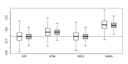
(i) FT

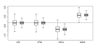
(ii) TF

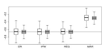
(iii) TT

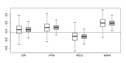
(iv) FF

Figure 2: Boxplots of estimators of the outcome mean.

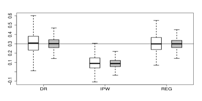
(i) FT

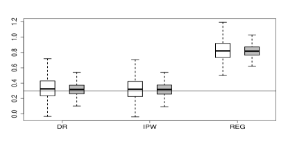
(ii) TF

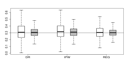
(iii) TT

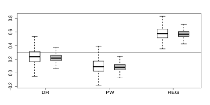
(iv) FF

Figure 3: Boxplots of estimators of the odds ratio parameter.

Note for Fig 3 and 3: Data are analyzed with four methods: doubly robust estimation (DR), regression based estimation (REG), inverse probability weighting (IPW), and the standard regression estimator (marREG) assuming MAR. In each boxplot, white boxes are for sample size 500, and gray ones for 1500. The horizontal line marks the true value of the parameter. FT stands for incorrect baseline propensity score and correct baseline outcome model, and the other three situations are similarly defined.

5.2 A Home Pricing example

We apply the proposed methods to a home pricing dataset extracted from the China Family Panel Studies. The dataset was collected from $3126$ households in China. The outcome of interest is log of current home price (in $10^{4}$ RMB yuan), of which $596$ $(21.8\%)$ values are missing, because the house owner does not respond in the survey, nor is the price available from the real estate market. Completely available covariates include log of construction price, province, urban ($1$ for urban household, $0$ rural), travel time to the nearest business center, house building area, family size, house story height, log of family income, and refurbish status.

The construction price of a house is related to the current price, however, we expect that it is independent of nonresponse conditional on the current price and fully observed covariates. Therefore, we use log of construction price as a shadow variable $Z$. Let $X$ denote the vector of all other covariates including the intercept, we assume the following models,

$$\text{\rm OR}(X,Y)=\exp(-\gamma Y),$$

$$\text{logit }f(R=1\mid X,Y=0)=X^{\rm T}\alpha,$$

$$E(Y\mid R=1,X,Z)=(X^{\rm T},Z)\beta_{1},$$

$$E(Z\mid R=1,X)=X^{\rm T}\beta_{2}.$$

We summarize estimates of the outcome mean and the odds ratio model in Table 2, and results for baseline models in Table S.1 in the Supplementary Material. Estimates for the odds ratio parameter produced by the proposed methods depart significantly from zero, providing empirical evidence of selection bias due to missingness and showing potential bias of standard estimation methods that assume MAR. The proposed methods result in slightly lower estimates of home price on the log scale than those obtained by standard methods assuming MAR; however, the deviation is more notable on the original scale and amount to significant bias equal to $1.26\times 10^{4}$ RMB yuan.

Table 2: The Home Pricing example.

		Outcome mean ($\psi$)							Odds ratio parameter ($\gamma$)
DR		2.604			(2.539, 2.669)				0.438			(0.270, 0.606)
REG		2.586			(2.518, 2.655)				0.745			(0.432, 1.064)
IPW		2.599			(2.534, 2.665)				0.413			(0.240, 0.585)
marREG		2.693			(2.637, 2.749)
marIPW		2.694			(2.638, 2.751)

Note: Point estimates and $95\%$ confidence intervals of the outcome mean and odds ratio parameter: marREG and marIPW respectively stand for standard regression estimation and inverse probability weighted estimation that assume MAR.

6 Semiparametric efficiency theory

6.1 The space of all influence functions

Asymptotic variances of the proposed estimators depend on the choice of the various user-specified functions $h(X,Z)$ indexing estimating equations. In this section, we study the efficiency of the estimators and derive the efficient influence function of the odds ratio parameter $\gamma$ and of the functional $\psi$, under the semiparametric model where the odds ratio model is correctly specified.

Let $f(Y,R\mid X,Z;\theta)$ denote a semiparametric or nonparametric model for the joint distribution of $(Y,R)$ conditional on $(X,Z)$, indexed by a possibly infinite-dimensional parameter $\theta$, which consists of two variation-independent components: $\theta=(\gamma,\eta)$, $\gamma$ for the odds ratio model $\text{\rm OR}(X,Y;\gamma)$ and $\eta$ for the baseline regression and the baseline propensity score. Although semiparametric efficiency is well studied under MAR, it is more challenging for MNAR data. In previous work, Robins, Rotnitzky and Scharfstein (2000); Rotnitzky and Robins (1997), and Vansteelandt, Rotnitzky and Robins (2007) have studied semiparametric efficiency for MNAR data assuming that

1. the odds ratio $\text{\rm OR}(X,Y,Z)$ is a completely known function.

Model (i) does not impose the shadow variable assumption as the odds ratio and the baseline propensity score may depend on $Z$. The approach of Robins, Rotnitzky and Scharfstein (2000) can be adapted by considering a shadow variable, that is,

1. the shadow variable Assumption 1 and the completeness Condition 1 hold; and the odds ratio function is completely known, i.e., $\text{\rm OR}(X,Y,Z)$ equals a given function $\text{\rm OR}(X,Y)$ for all $(X,Y,Z)$;

however, this model is not entirely of interest because the exact odds ratio function is seldom known in practice.

In contrast, we consider a more general model which allows for uncertainty of the odds ratio function:

1. the shadow variable Assumption 1 and the completeness Condition 1 hold; and the odds ratio function follows a parametric model, i.e., $\text{\rm OR}(X,Y,Z)=\text{\rm OR}(X,Y;\gamma)$ with an unknown and finite dimensional parameter $\gamma$.

Model (ii) is a generalization of (i*) by allowing for unknown selection bias. In (ii), the baseline regression and the baseline propensity score remain nonparametric, and thus (ii) in fact contains a large class of semiparametric models for the joint distribution. Model (ii) is different from the semiparametric models of Zhao and Ma (2019) who requires a fully parametric model for $f(Y\mid X,Z)$ and leaves the propensity score $f(R=1\mid X,Y)$ nonparametric; model (ii) is more general than the model of Morikawa and Kim (2016) who considers a fully parametric propensity score model that in fact specifies parametric forms for both the odds ratio function $\text{\rm OR}(X,Y)$ and the baseline propensity score $f(R=1\mid X,Y=0)$.

Consider a full data functional $\psi$ that solves a given estimating equation $E\{U(X,Y,Z;\psi)\}=0$, we wish to derive the set of influence functions for all regular and asymptotically linear (RAL) estimators of $\psi$ assuming (ii), and to characterize the semiparametric efficiency bound for model (ii). We let ${\rm NIF}(\psi,\theta)$ denote the full data influence function for $\psi$ in the nonparametric model of $f(Y,R\mid X,Z)$, for example, ${\rm NIF}(\psi,\theta)=Y-\psi$ for $\psi=E(Y)$. For notational simplicity, we use $w=w(X,Y)=1/f(R=1\mid X,Y)$ to denote the inverse probability weight. Let $\mathcal{H}^{(X,Z)}$ denotes a generic Hilbert space consisting of all measurable vector functions $h(X,Z)$ of $(X,Z)$ with finite variance equipped with the covariance inner product. The dimension of the vector function $h$ is conformable to the parameter appearing in the corresponding estimating equation. We denote

$${\rm IF}_{0}(\psi,\theta)=wR\cdot{\rm NIF}(\psi,\theta)+(1-wR)E\{{\rm NIF}(\psi,\theta)\mid R=0,X\},$$

and for arbitrary $h\in\mathcal{H}^{(X,Z)}$, we denote

$$T(h;\theta)=(1-wR)\{h-E(h\mid R=0,X)\},$$

$${\rm IF}_{1}(h;\psi,\theta)={\rm IF}_{0}(\psi,\theta)+T(h;\theta).$$

One can verify that ${\rm IF}_{0}(\psi,\theta)$ is in fact an observed data influence function for $\psi$ under model (i*), i.e., when $\gamma$ is known; and in the Supplementary Material, we show that the orthogonal complement to the observed data tangent space under (i*), denoted by $\mathcal{T}^{\bot}$, is

$$\mathcal{T}^{\bot}=\{T(h;\theta)\text{ for all }h\in\mathcal{H}^{(X,Z)}\};$$

and the space of all observed data influence functions for $\psi$ under (i*) is

$$\{{\rm IF}_{1}(h;\psi,\theta)\text{ for all }h\in\mathcal{H}^{(X,Z)}\}.$$

However, results derived under (i*) do not account for the uncertainty about the unknown odds ratio model. Under model (ii) allowing for a parametric odds ratio model with unknown parameters, we have the following results.

Theorem 3.

Under model (ii) and the regularity conditions described by Bickel et al. (1993), we have that

• the observed data score function of $\gamma$ is

  $$S_{\gamma}=\{f(R=1\mid X,Z)-R\}E\{\nabla_{\gamma}\log\text{\rm OR}(X,Y;\gamma)\mid R=0,X,Z\};$$

  and the set of influence functions for all RAL estimators of $\gamma$ is

  $$\{{\rm IF}_{\gamma}(g;\theta)=[E\{T(g;\theta)S_{\gamma}^{\rm T}\}]^{-1}\cdot T(g;\theta):T(g;\theta)\in\mathcal{T}^{\bot}\};$$

• the set of influence functions for all RAL estimators of $\psi$ is

  $$\left\{\begin{array}[]{c}{\rm IF}_{2}(g,h;\psi,\theta)={\rm IF}_{1}(h;\psi,\theta)+E\{\nabla_{\gamma}{\rm IF}_{1}(h;\psi,\theta)\}\cdot{\rm IF}_{\gamma}(g;\theta),\\ \text{for all $g,h$}\in\mathcal{H}^{(X,Z)}\end{array}\right\}.$$

Theorem 3 shows the impact of the odds ratio model on the influence functions of $\psi$. As a special case, when the odds ratio function is completely known as in (i) or (i*), we have ${\rm IF}_{2}(g,h;\psi,\theta)={\rm IF}_{1}(h;\psi,\theta)$; if further the missingness is at random, i.e., $\text{\rm OR}(X,Y)=1$ for all $(X,Y)$, then ${\rm IF}_{1}(h;\psi,\theta)$ becomes an influence function under MAR.

6.2 The efficient influence function

We let $\Pi(\cdot\mid\mathcal{T}^{\bot})$ denote the orthogonal projection onto $\mathcal{T}^{\bot}$, the orthogonal complement to the observed data tangent space in model (i*). The following result gives the efficient influence function.

Theorem 4.

Under model (ii), we have that

1. the efficient influence function for $\gamma$ is

   $${\rm EIF}_{\gamma}(\theta)=\{E(S^{\rm eff}_{\gamma}(S^{\rm eff}_{\gamma})^{\rm T})\}^{-1}S_{\gamma}^{\rm eff},$$

   with $S_{\gamma}^{\rm eff}=\Pi(S_{\gamma}\mid\mathcal{T}^{\bot})$ the efficient score of $\gamma$;

2. the efficient influence function for $\psi$ is

   $${\rm EIF}_{\psi}(\psi,\theta)={\rm IF}_{1}^{\rm eff}(\psi,\theta)+E\{\nabla_{\gamma}{\rm IF}_{1}^{\rm eff}(\psi,\theta)\}\cdot{\rm EIF}_{\gamma}(\theta),$$

   with

   $${\rm IF}_{1}^{\rm eff}(\psi,\theta)={\rm IF}_{0}(\psi,\theta)-\Pi\{{\rm IF}_{0}(\psi,\theta)\mid\mathcal{T}^{\bot}\}.$$

As shown in (b), ${\rm IF}_{1}^{\rm eff}(\psi,\theta)$ is in fact the efficient influence function of $\psi$ in model (i*) where the odds ratio parameter $\gamma$ is known; by taking account of the impact of estimating $\gamma$, which is captured by $E\{\nabla_{\gamma}{\rm IF}_{1}^{\rm eff}(\psi,\theta)\}\cdot{\rm EIF}_{\gamma}(\theta)$, we obtain the efficient influence function of $\psi$ in model (ii). The efficient influence function involves the projection $\Pi(\cdot\mid\mathcal{T}^{\bot})$, which is in general complicated. Nonetheless, we show that this is available in closed form as summarized below.

Theorem 5.

Under model (ii), any function of the observed data can be written as $m(RY,R,X,Z)=(1-R)m_{0}(X,Z)+R\cdot m_{1}(X,Y,Z)$, and we have that

$$\Pi(m\mid\mathcal{T}^{\bot})=(1-wR)\left\{K-\frac{Q\cdot E(K\mid R=0,X)}{E(Q\mid R=0,X)}\right\},$$

with

$$Q = 1/E\{w\mid R=0,X,Z\},$$

$$K = Q\cdot E(m_{0}-m_{1}\mid R=0,X,Z).$$

For illustration, in the Supplementary Material we derive the efficient influence function when both $Y$ and $Z$ are binary.

Corollary 1.

Consider binary $Y$ and $Z$, then under model (ii), we have that

$$S_{\gamma}^{\rm eff}=(1-wR)\{Z-E(Z\mid R=0,X)\}\frac{(G_{1}-G_{0})\nabla_{\gamma}\log\text{\rm OR}(X,Y=1;\gamma)}{E(w\mid R=0,X)},$$

with $G_{z}=E(Y\mid R=0,X,Z=z)$ for $z=0,1$, and that

$$\Pi({\rm IF}_{0}\mid\mathcal{T}^{\bot})=(1-wR)\{Z-E(Z\mid R=0,X)\}\frac{H_{1}-H_{0}}{E(w\mid R=0,X)},$$

with $H_{z}=E[w\{E({\rm NIF}\mid R=0,X)-{\rm NIF}\}\mid R=0,X,Z=z]$ for $z=0,1$.

Theorems 4–5 provide a theoretical efficiency bound for all RAL estimators of $\psi$ in model (ii), and offer a closed form for the efficient influence function. Consider the union model $M_{1}$$\cup$$M_{2}$ that assumes either ($M_{1}$) $f(Y,Z\mid R=1,X;\beta)$ and $\text{\rm OR}(X,Y;\gamma)$ are correctly specified, or ($M_{2}$) $f(R=1\mid Y=0,X;\alpha)$ and $\text{\rm OR}(X,Y;\gamma)$ are correctly specified. General results of Robins and Rotnitzky (2001) imply that in the aforementioned union model $M_{1}$$\cup$$M_{2}$, ${\rm EIF}_{\psi}$ and ${\rm EIF}_{\gamma}$ are also the efficient influence functions for $\psi$ and $\gamma$, respectively. It follows that $\hat{\gamma}^{\rm eff}$, the solution to $\hat{E}\{{\rm EIF}_{\gamma}(\gamma,\hat{\alpha},\hat{\beta})\}=0$ and $\hat{\psi}^{\rm eff}$ the solution to $\hat{E}\{{\rm EIF}(\psi,\hat{\alpha},\hat{\beta},\hat{\gamma})\}=0$ with $\hat{\alpha},\hat{\beta},\hat{\gamma}$ estimates of the nuisance parameters, are locally semiparametric efficient in the union model $M_{1}\cup M_{2}$ at the intersection submodel $M_{1}\cap M_{2}$; that is, $\hat{\gamma}^{\rm eff}$ and $\hat{\psi}^{\rm eff}$ attain the semiparametric efficiency bound for the union model when both baseline models happen to hold.

Under the union model, the efficient estimator can also be obtained based on an initial doubly robust $\sqrt{n}$-consistent estimator $(\hat{\psi},\hat{\gamma})$ by a one-step construction following Bickel et al. (1993),

$$\hat{\gamma}^{\rm eff}=\hat{\gamma}+\hat{E}\{{\rm EIF}_{\gamma}(\hat{\alpha},\hat{\beta},\hat{\gamma})\},$$

$$\hat{\psi}^{\rm eff}=\hat{\psi}+\hat{E}\{{\rm EIF}(\hat{\psi},\hat{\alpha},\hat{\beta},\hat{\gamma})\}.$$

7 Discussion

We have developed a general semiparametric framework for identification and inference about any functional of the full data law in the presence of nonignorable missing outcome data with the aid of a shadow variable. Under certain completeness condition, we describe the largest class of nonoparametric models that are identifiable by the approach. Our approach reveals the central role of the odds ratio function and the shadow variable in identification of full data distribution. The identification conditions we propose only involve the observed data, and thus can be justified empirically. Our identification results establish the basis for statistical inference in both this paper and a recently published companion paper (Miao and Tchetgen Tchetgen, 2016), which builds directly on a prior draft of the current manuscript. When the shadow variable Assumption 1 does not hold, the odds ratio function is in general not identified, and one can conduct sensitivity analysis to check how results would change according to the impact of the shadow variable. We refer to Robins, Rotnitzky and Scharfstein (2000) for details for sensitivity analysis. The proposed identification, estimation, and semiparametric efficiency theory readily extends to missing covariate problems considered by Miao and Tchetgen Tchetgen (2018) and Yang, Wang and Ding (2019), who employ a shadow variable identifying condition, however do not provide a framework for semiparametric inference. The proposed methods can also be extended to longitudinal data analysis, which is often subject to dropout or missing data. Their potential use for such complicated settings will be studied elsewhere.

Appendix

Proof of Theorem 1.

Under the shadow variable Assumption 1, from Proposition 1 we have

$$E\{\widetilde{\text{\rm OR}}(X,Y)\mid R=1,X,Z\}=\frac{f(Z\mid R=0,X)}{f(Z\mid R=1,X)},$$ (A.1)

$$\widetilde{\text{\rm OR}}(X,Y)=\frac{\text{\rm OR}(X,Y)}{E\{\text{\rm OR}(X,Y)\mid R=1,X\}}.$$

Based on these two equalities, we prove identification of $\text{\rm OR}(X,Y)$ under Assumption 1. Because $f(Y\mid R=1,X,Z)$ and $f(Z\mid R=1,X)$ can be obtained from the observed data, for any candidate of $\text{\rm OR}(X,Y)$, $E\{\widetilde{\text{\rm OR}}(X,Y)\mid R=1,X,Z\}$ can be computed from the observed data. Suppose $\text{\rm OR}^{*}(X,Y)$ is the truth and $\text{\rm OR}^{\prime}(X,Y)$ is a candidate that

$$E\{\widetilde{\text{\rm OR}}^{\prime}(X,Y)\mid R=1,X,Z\}=\frac{f(Z\mid R=0,X)}{f(Z\mid R=1,X)}.$$

We have

$$E\{\widetilde{\text{\rm OR}}^{\prime}(X,Y)-\widetilde{\text{\rm OR}}^{*}(X,Y)\mid R=1,X,Z\}=0,$$

which together with Condition 1 implies that $\widetilde{\text{\rm OR}}^{\prime}(X,Y)=\widetilde{\text{\rm OR}}^{*}(X,Y)$. Therefore, (A.1) must have a unique solution, that is, $\widetilde{\text{\rm OR}}(X,Y)$ is identified and hence $\text{\rm OR}(X,Y)$ is identified by $\text{\rm OR}(X,Y)=\widetilde{\text{\rm OR}}(X,Y)/\widetilde{\text{\rm OR}}(X,Y=0)$. ∎

Proof of Theorem 2 rests on the following lemma.

Lemma A.1.

Under Assumptions 1, for any square integrable function $g(X,Y,Z)$, we have

$$E[\{w(X,Y)R-1\}g(X,Y,Z)]=0,$$ (A.2)

$$E[R\cdot\text{\rm OR}(X,Y)\{g(X,Y,Z)-E(g(X,Y,Z)\mid R=0,X)\}]=0,$$ (A.3)

$$E[R\cdot\text{\rm OR}(X,Y)\{g(X,Y,Z)-E(g(X,Y,Z)\mid R=0,X,Z)\}]=0.$$ (A.4)

Proof.

From Assumption 1, $Z\begin{picture}(9.0,8.0)\put(0.0,0.0){\line(1,0){9.0}} \put(3.0,0.0){\line(0,1){8.0}} \put(6.0,0.0){\line(0,1){8.0}} \end{picture}R\mid(X,Y)$ implies that for any function $g(X,Y,Z)$,

$${E}\{[w(X,Y)R-1]g(X,Y,Z)\mid X,Y\}$$

$$= E\{w(X,Y)f(R=1\mid X,Y)-1\}{E}\{g(X,Y,Z)\mid X,Y\}$$

$$= 0.$$

and thus $E[\{w(X,Y)R-1\}g(X,Y,Z)]=0$.

From (6) and (7), we have

$$f(Y,Z\mid R=0,X)=\frac{\text{\rm OR}(X,Y)f(Y,Z\mid R=1,X)}{E[\text{\rm OR}(X,Y)\mid R=1,X]},$$

and thus for any function $g(X,Y,Z)$,

$${E}\{g(X,Y,Z)\mid R=0,X\} = \frac{E\{R\cdot\text{\rm OR}(X,Y)\cdot g(X,Y,Z)\mid X\}}{E\{R\cdot\text{\rm OR}(X,Y)\mid X\}}.$$

So we have

$$E[R\cdot\text{\rm OR}(X,Y)\{g(X,Y,Z)-E(g(X,Y,Z)\mid R=0,X)\}\mid X]=0,$$

and thus,

$$E[R\cdot\text{\rm OR}(X,Y)\{g(X,Y,Z)-E(g(X,Y,Z)\mid R=0,X)\}]=0.$$

Therefore, (A.3) holds, and (A.4) holds because (A.3) implies that for any $g(X,Y,Z)$,

$$E[R\cdot\text{\rm OR}(X,Y)\{E(g(X,Y,Z)\mid R=0,X,Z)-E(g(X,Y,Z)\mid R=0,X)\}]=0.$$

∎

Proof of Theorem 2.

We only need to show unbiasedness of the estimating equations, and then following from the general theory of estimating equations, consistency and asymptotic normality of the estimators hold under the regularity conditions described by Newey and McFadden (1994).

(a). Applying Lemma A.1 with $g(X,Y,Z)=h(X,Z)$ and $g(X,Y,Z)=U(\psi)=U(X,Y,Z;\psi)$, respectively, we obtain that under the true values of $(\alpha,\gamma,\psi)$,

$$E[\{w(X,Y;\alpha,\gamma)R-1\}h(X,Z)]=0,$$

and

$$E[\{w(X,Y;\alpha,\gamma)R-1\}U(\psi)]=0,$$

which imply that (11) and (12) are unbiased estimating equations for $(\alpha,\gamma)$ and $\psi$, respectively.

(b). Under a correct baseline regression model $f(Y,Z\mid R=1,X;\beta)$, it is obvious that the complete-case score equation is unbiased at the true value of $\beta$, i.e.,

$$E\{R\cdot S(X,Y,Z;\beta)\}=0.$$

Further given correctly specified odds ratio model $\text{\rm OR}(X,Y;\gamma)$, we have that for any function $g(X,Y,Z)$,

$${E}\{(1-R)g(X,Y,Z)\mid X\}={E}[(1-R){E}\{g(X,Y,Z)\mid R=0,X;\beta,\gamma\}\mid X],$$

thus,

$$E[(1-R)\{g(X,Y,Z)-E(g(X,Y,Z)\mid R=0,X;\beta,\gamma)\}]=0.$$

As special cases, the above equation holds for $g(X,Y,Z)=h(X,Z)$ and $g(X,Y,Z)=U(\psi)$, that is, (9) and (10) are unbiased estimating equations for $\gamma$ and $\psi$, respectively.

(c). We show that if either model ($M_{1}$) or ($M_{2}$) holds, (13) and (14) are unbiased estimating equations for $\gamma$ and $\psi$, respectively.

(c1). Suppose $\text{\rm OR}(X,Y;\gamma)$ and $f(R=1\mid X,Y=0;\alpha)$ are correctly specified, but $f(Y,Z\mid R=1,X;\beta)$ may not be. We let $\beta^{*}$ denote the probability limit of $\hat{\beta}$. Applying Lemma A.1 with $g(X,Y,Z)=h(X,Z)-\tilde{E}(h(X,Z)\mid R=0,X;\beta^{*},\gamma)$, we have that at $\beta^{*}$ and the true value of $(\alpha,\gamma)$,

$$E[\{w(X,Y;\alpha,\gamma)R-1\}\{h(X,Z)-\tilde{E}(h(X,Z)\mid R=0,X;\beta^{*},\gamma)\}]=0.$$

Thus, (13) is an unbiased estimating equation for $(\alpha,\gamma)$. Applying Lemma A.1 with $g(X,Y,Z)=U(\psi)-\tilde{E}\{U(\psi)\mid R=0,X,Z;\beta^{*},\gamma\}$, we have that at $\beta^{*}$ and the true value of $(\alpha,\gamma,\psi)$,

$$E[\{w(X,Y;\alpha,\gamma)R-1\}\{U(\psi)-\tilde{E}[U(\psi)\mid R=0,X,Z;\beta^{*},\gamma]\}]=0.$$

and thus, (14) is an unbiased estimating equation for $\psi$.

(c2). Suppose $\text{\rm OR}(X,Y;\gamma)$ and $f(Y,Z\mid R=1,X;\beta)$ are correctly specified, but $f(R=1\mid X,Y=0;\alpha)$ may not be. We let $\alpha^{*}$ denote the probability limit of $\hat{\alpha}$. Under a correct baseline regression model $f(Y,Z\mid R=1,X;\beta)$, (8) is an unbiased estimating equation for $\beta$. Note that at $\alpha^{*}$ and the true value of $(\beta,\gamma)$,

$$E[\{w(X,Y;\alpha^{*},\gamma)R-1\}\{h(X,Z)-E[h(X,Z)\mid R=0,X;\beta,\gamma]\}]$$

$$= E[R\{w(X,Y;\alpha^{*},\gamma)-1\}\{h(X,Z)-{E}[h(X,Z)\mid R=0,X;\beta,\gamma]\}]$$

$$-{E}[(1-R)\{h(X,Z)-{E}[h(X,Z)\mid R=0,X;\beta,\gamma]\}].$$

As we have proved in Theorem 2 (b), the second term of the right hand side equals zero. We only need to show that the first term also equals zero. Note that

$$R\{w(X,Y;\alpha^{*},\gamma)-1\}=R\times\text{\rm OR}(X,Y;\gamma)\frac{f(R=0\mid X,Y=0;\alpha^{*})}{f(R=1\mid X,Y=0;\alpha^{*})},$$

applying Lemma A.1 with

$$g(X,Y,Z)=\frac{f(R=0\mid X,Y=0;\alpha^{*})}{f(R=1\mid X,Y=0;\alpha^{*})}\biggl{.}\biggl{.}\{h(X,Z)-E[h(X,Z)\mid R=0,X;\beta,\gamma]\},$$

(A.3) implies that the first term on the right hand side of (Proof of Theorem 2.) also equals zero. As a result, (Proof of Theorem 2.) must equal zero at the true values of $(\beta,\gamma)$. In addition, letting $g(X,Y,Z)=U(\psi)$, (A.4) implies that at $\alpha^{*}$ and the true values of $(\beta,\gamma,\psi)$,

$${E}[\{w(X,Y;\alpha^{*},\gamma)R-1\}\{U(\psi)-E[U(\psi)\mid R=0,X,Z;\beta,\gamma]\}]=0,$$

Therefore, (8), (13), and (14) are unbiased estimating equations for $(\beta,\gamma,\psi)$.

In summary, if either model ($M_{1}$) or ($M_{2}$) is correct, (13) and (14) are unbiased estimating equations for $(\gamma,\psi)$.

∎

We need the following lemma to prove Theorem 3.

Lemma A.2.

Under model (i*), the ortho-complement to the observed data tangent space is

$$\mathcal{T}^{\bot}=\left\{\begin{array}[]{c}T(h;\theta)\text{ for any }h=h(X,Z)\in\mathcal{H}^{(X,Z)}\end{array}\right\},$$ (A.6)

with

$$T(h;\theta)=\{1-wR\}\{h-E(h\mid R=0,X)\}.$$

We prove this lemma in the Supplementary Material. Let ${\rm NIF}(\psi,\theta)$ denote the full data influence function of $\psi$ in the nonparametric model $f(X,Y,Z;\theta)$. One can verify that

$${\rm IF}_{0}(\psi,\theta)=wR\cdot{\rm NIF}(\psi,\theta)+(1-wR)E\{{\rm NIF}(\psi,\theta)\mid R=0,X\},$$

is an observed data influence function for $\psi$ in model (i*), then according to Newey (1994) we have the set of all observed data influence functions under (i*), which is ${\rm IF}_{0}(\psi,\theta)+\mathcal{T}^{\bot}$.

Corollary 2.

In model (i*), the set of influence functions for all RAL estimators of $\psi$ is ${\rm IF}_{0}(\psi,\theta)+\mathcal{T}^{\bot}$, i.e.,

$$\left\{\begin{array}[]{c}{\rm IF}_{1}(h;\psi,\theta)={\rm IF}_{0}(\psi,\theta)+T(h;\theta)\text{ for arbitrary }h=h(X,Z)\in\mathcal{H}^{(X,Z)}.\\ \end{array}\right\}$$

Proof of Theorem 3.

We prove that the results hold within all parametric submodels of the semiparametric model, and then the results hold for the semiparametric model by aggregating all submodels. Consider a one-dimensional parametric submodel $f(Y,R\mid X,Z;\theta_{t})$ indexed by $t$, i.e., a path in the semiparametric model (ii), with $\theta_{t}=(\gamma_{t},\eta_{t})$ and $\theta_{0}$ equal to the true value $\theta$. We let $S_{t}$ denote the observed data score function in the submodel; we use $\Pi(\cdot\mid\mathcal{T}^{\bot})$ to denote the projection onto $\mathcal{T}^{\bot}$.

1. We first derive the observed data score function $S_{\gamma}$. The full data likelihood $f(Y,R\mid X,Z;\gamma)$ can be written as

   $$\frac{f(R\mid X,Y=0)f(Y\mid R=1,X,Z)\text{\rm OR}(X,Y;\gamma)^{1-R}}{\int f(R\mid X,Y=0)f(Y\mid R=1,X,Z)\text{\rm OR}(X,Y;\gamma)^{1-R}dRdY},$$

   and the observed data likelihood is

   $$\{f(Y,R=1\mid X,Z;\gamma)\}^{R}\{f(R=0\mid X,Z;\gamma)\}^{1-R};$$

   then the full data score function of $\gamma$ is

   $$S_{\gamma}^{\rm F}=(1-R)\nabla_{\gamma}\log\text{\rm OR}(X,Y;\gamma)-E\{(1-R)\nabla_{\gamma}\log\text{\rm OR}(X,Y;\gamma)\mid X,Z\},$$

   and the observed data score function of $\gamma$ is

   $$S_{\gamma}=R\cdot S_{\gamma}^{\rm F}+(1-R)E\{S_{\gamma}^{\rm F}\mid R=0,X,Z\}.$$

   After some algebra, we can verify that

   $$S_{\gamma}=\{f(R=1\mid X,Z)-R\}E\{\nabla_{\gamma}\log\text{\rm OR}(X,Y;\gamma)\mid R=0,X,Z\}.$$

   Next, following from the fact that the orthogonal complement to the nuisance tangent space under model (ii) is exactly the space $\mathcal{T}^{\bot}$, and therefore from Tsiatis (2006, Theorem 4.2), the space of influence functions for all RAL estimator for $\gamma$ is

   $$\{{\rm IF}_{\gamma}(g;\theta)=[E\{T(g;\theta)S_{\gamma}^{\rm T}\}]^{-1}T(g;\theta):T(g;\theta)\in\mathcal{T}^{\bot}\}.$$ (A.8)

2. For any $t$ and $h=h(X,Z)$, we let $\psi_{t}$ denote the solution to

   $$E_{t}\{{\rm IF}_{1}(h;\psi_{t},\theta_{t})\}=0,$$

   where $E_{t}$ denotes expectation with respect to $f(Y,R\mid X,Z;\theta_{t})$. Therefore, we have that

   $$0 =\nabla_{t}E_{t}\{{\rm IF}_{1}(h;\psi_{t},\theta_{t})\}$$ (A.9)

   $$=E\{{\rm IF}_{1}(h;\psi,\theta)S_{t}\}+E\{\nabla_{t}{\rm IF}_{1}(h;\psi_{t},\theta_{t})\}$$

   $$=E\{{\rm IF}_{1}(h;\psi,\theta)S_{t}\}+E\{\nabla_{\psi}{\rm IF}_{1}(h;\psi,\theta)\}\nabla_{t}\psi_{t}$$

   $$\quad+E\{\nabla_{\gamma}{\rm IF}_{1}(h;\psi,\theta)\}\nabla_{t}\gamma_{t}+E\{\nabla_{\eta}{\rm IF}_{1}(h;\psi,\theta)\}\nabla_{t}\eta_{t}.$$

   In order to derive the form of influence functions for $\psi$ under model (ii), we prove that $E\{\nabla_{\eta}{\rm IF}_{1}(h;\psi,\theta)\}=0$ by separately showing that $E\{\nabla_{\eta}{\rm IF}_{0}(h,\psi,\theta)\}=0$ and that $E\{\nabla_{\eta}T(h;\theta)\}=0$ for all $h=h(X,Z)$. Let $\eta_{i}$ denote the $i$th component of $\eta$ and $\eta_{-i}$ the others. A similar argument to the proof of Theorem 2 (c) indicates double robustness of ${\rm IF}_{0}(h;\psi,\theta)$ against misspecification of the baseline model parameters $\eta$, that is, for all $\eta_{i}+\delta_{i}$ in an open neighborhood of $\eta_{i}$, $E\{{\rm IF}_{0}(h;\psi,\gamma,\eta_{i}+\delta_{i},\eta_{-i})\}=0$. We thus have

   $$E\{\nabla_{\eta_{i}}{\rm IF}_{0}(h;\psi,\theta)\}$$

   $$=E_{\theta}\left\{\lim_{\delta_{i}\rightarrow 0}\frac{{\rm IF}_{0}(h;\psi,\gamma,\eta_{i}+\delta_{i},\eta_{-i})-{\rm IF}_{0}(h;\psi,\gamma,\eta_{i},\eta_{-i})}{\delta_{i}}\right\}$$

   $$=\lim_{\delta_{i}\rightarrow 0}E\left\{\frac{{\rm IF}_{0}(h;\psi,\gamma,\eta_{i}+\delta_{i},\eta_{-i})-{\rm IF}_{0}(h;\psi,\gamma,\eta_{i},\eta_{-i})}{\delta_{i}}\right\}=0.$$

   Therefore, we have $E\{\nabla_{\eta}{\rm IF}_{0}(h;\psi,\theta)\}=0$.

   Given $\gamma$, Lemma A.2 implies that $E\{T(h;\theta)S_{\eta}\}=0$ for any $T(h;\theta)\in\mathcal{T}^{\bot}$. Thus, $E\{\nabla_{\eta}T(h;\theta)\}=-E\{T(h;\theta)S_{\eta}\}=0$, and as a result,

   $$E\{\nabla_{\eta}{\rm IF}_{1}(h;\psi,\theta)\}=0.$$ (A.10)

   In addition, because for any $h$, ${\rm IF}_{1}(h;\psi,\theta)$ is an influence function for $\psi$ when $\gamma$ is known, we have that

   $$E\{\nabla_{\psi}{\rm IF}_{1}(h;\psi,\theta)\}=-1.$$ (A.11)

   Newey (1994) shows that for any influence function ${\rm IF}_{\gamma}$ of $\gamma$,

   $$\nabla_{t}\gamma_{t}=E({\rm IF}_{\gamma}S_{t}).$$ (A.12)

   From (A.9)–(A.12), we have

   $$\nabla_{t}\psi_{t}=E[\{{\rm IF}_{1}(h;\psi,\theta)+E(\nabla_{\gamma}{\rm IF}_{1}(h;\psi,\theta))\cdot{\rm IF}_{\gamma}(g;\theta)\}S_{t}],$$

   which implies from Newey (1994) that for any $h$ and $g\in\mathcal{H}^{(X,Z)}$,

   $${\rm IF}_{2}(h,g;\psi,\theta)={\rm IF}_{1}(h;\psi,\theta)+E\{\nabla_{\gamma}{\rm IF}_{1}(h;\psi,\theta)\}\cdot{\rm IF}_{\gamma}(g;\theta)$$ (A.13)

   is an influence function for $\psi$ in model (ii).

   In fact, (A.13) represents all influence functions for $\psi$ in model (ii) as we demonstrate below. Given any $h_{0}(X,Z),g_{0}(X,Z)$, Newey (1994) implies that the following linear variety is the set of all influence functions for $\psi$ assuming (ii),

   $${\rm IF}_{2}(h_{0},g_{0};\psi,\theta)+\text{ ortho-complement to the tangent space assuming (ii)}.$$

   Moreover, the ortho-complement to the tangent space under model (ii) can be represented as $\{T(h;\theta)\in\mathcal{T}:E\{T(h;\theta)\cdot S_{\gamma}\}=0\}$, which is equivalent to

   $$\{T(h;\theta)\in\mathcal{T}:E\{\nabla_{\gamma}T(h;\theta)\}=0\},$$

   by noting that $E\{\nabla_{\gamma}T(h;\theta)\}=-E\{T(h;\theta)\cdot S_{\gamma}\}$. Therefore, the space of all influence functions for $\psi$ assuming (ii) is

   $$\{{\rm IF}_{2}(h_{0},g_{0};\psi,\theta)+T(h;\theta)\}\text{ for all $T(h;\theta)\in\mathcal{T}$ and }E\{\nabla_{\gamma}T(h;\theta)\}=0,$$

   that is,

   $${\rm IF}_{2}(h_{0},g_{0};\psi,\theta)+T(h;\theta)$$

   $$= {\rm IF}_{1}(h_{0};\psi,\theta)+E\{\nabla_{\gamma}{\rm IF}_{1}(h_{0};\psi,\theta)\}\cdot{\rm IF}_{\gamma}(g_{0};\theta)+T(h;\theta)$$

   $$= {\rm IF}_{1}(h_{0}+h;\psi,\theta)+E\{\nabla_{\gamma}{\rm IF}_{1}(h_{0};\psi,\theta)\}\cdot{\rm IF}_{\gamma}(g_{0};\theta)$$

   $$= {\rm IF}_{1}(h_{0}+h;\psi,\theta)+E\{\nabla_{\gamma}{\rm IF}_{1}(h_{0}+h;\psi,\theta)\}\cdot{\rm IF}_{\gamma}(g_{0};\theta)$$

   $$= {\rm IF}_{2}(h_{0}+h,g_{0};\psi,\theta).$$

   As a result, any influence function for $\psi$ assuming (ii) can be represented in the form of (A.13).

∎

Proof of Theorem 4.

• This is implied from the result of Tsiatis (2006, Theorem 4.2) that ${\rm EIF}_{\gamma}(\theta)=\{E(S^{\rm eff}_{\gamma}(S^{\rm eff}_{\gamma})^{\rm T})\}^{-1}S_{\gamma}^{\rm eff}$, with $S_{\gamma}^{\rm eff}=\Pi(S_{\gamma}\mid\mathcal{T}^{\bot})$.

• To derive the efficient influence function for $\psi$, we choose $g$ and $h$ such that ${\rm IF}_{2}(g,h;\psi,\theta)$ falls in the observed data tangent space under model (ii). Because $\Pi({\rm IF}_{0}\mid\mathcal{T}^{\bot})\in\mathcal{T}^{\bot}$, there exists $h^{\rm eff}(X,Z)$ such that $T(h^{\rm eff})=-\Pi({\rm IF}_{0}\mid\mathcal{T}^{\bot})$, and we let ${\rm IF}_{1}^{\rm eff}={\rm IF}_{0}+T(h^{\rm eff})=\Pi({\rm IF}_{0}\mid\mathcal{T})$. We further choose $g^{\rm eff}(X,Z)$ such that ${\rm EIF}_{\gamma}=T(g^{\rm eff})$ is the efficient influence function for $\gamma$. Then we have that

  $${\rm EIF}_{\psi} = {\rm IF}_{1}^{\rm eff}(\psi,\theta)+E\{\nabla_{\gamma}{\rm IF}_{1}^{\rm eff}(\psi,\theta)\}\cdot{\rm EIF}_{\gamma}$$

  $$= \Pi({\rm IF}_{0}\mid\mathcal{T})+E\{\nabla_{\gamma}\Pi({\rm IF}_{0}\mid\mathcal{T})\}\cdot T(g^{\rm eff}).$$

  Note that $\mathcal{T}$ is the observed data tangent space assuming (i*), and it is contained in the observed data tangent space assuming (ii). Hence, $T(g^{\rm eff})$ and $\Pi({\rm IF}_{0}\mid\mathcal{T})$ belong to the latter space and so does ${\rm EIF}_{\psi}$. Therefore, ${\rm EIF}_{\psi}$ is the efficient influence function for $\psi$.

∎

Proof of Theorem 5.

Consider the space $\mathcal{T}^{\bot}=\{T(h):h=h(X,Z)\in\mathcal{H}^{(X,Z)}\}$, with

$$T(h) = \{1-wR\}\{h-E[h\mid R=0,X]\}$$

$$= \{(1-R)-R(w-1)\}\{h-E(h\mid R=0,X)\}.$$

We show how to project onto the space $\mathcal{T}^{\bot}$, that is, we wish to find $T(h^{*})=\Pi(m\mid\mathcal{T}^{\bot})$ for any function $m=m(RY,R,X,Z)$ of the observed data. First note that for any $m,$ there exist a function $m_{0}$ of $(X,Z)$ and $m_{1}$ of $(X,Y,Z)$, such that $m(RY,R,X,Z)=(1-R)m_{0}(X,Z)+Rm_{1}(X,Y,Z).$ We therefore wish to find $h^{*}=h^{*}(X,Z)$ that solves

$$E[\{m-T(h^{*})\}T(h)]=0\text{ for all $h=h(X,Z)\in\mathcal{H}^{X,Z}$}.$$ (A.15)

For any $h=h(X,Z)$, letting $\Delta(h)=h-E(h\mid X,R=0)$, we have that

$$0 = E[\{m-T(h^{*})\}T(h)]$$

$$= E\left[\begin{array}[]{c}\{(1-R)m_{0}+Rm_{1}-((1-R)-R(w-1))\Delta(h^{*})\}\\ \cdot\{(1-R)-R(w-1)\}\Delta(h)\end{array}\right]$$

$$= E\left\{\begin{array}[]{c}(1-R)m_{0}\Delta(h)-m_{1}R(w-1)\cdot\Delta(h)-(1-R)\Delta(h)\Delta(h^{*})\\ -R(w-1)^{2}\Delta(h^{*})\Delta(h)\end{array}\right\}$$

note that $$R(w-1)=1-R-(1-wR)$$, applying (A.2) we have

$$= E\left\{\begin{array}[]{c}(1-R)m_{0}\Delta(h)-(1-R)m_{1}\Delta(h)-(1-R)\Delta(h^{*})\Delta(h)\\ -(1-R)(w-1)\cdot\Delta(h^{*})\Delta(h)\end{array}\right\}$$

$$= E[\{m_{0}-m_{1}-w\Delta(h^{*})\}\cdot\{(1-R)\Delta(h)\}]$$

$$= E\left[E\{m_{0}-m_{1}-w\Delta(h^{*})\mid R=0,X,Z\}\cdot\{(1-R)\Delta(h)\}\right]$$

$$= E\left[\Delta(E\{m_{0}-m_{1}-w\Delta(h^{*})\mid R=0,X,Z\})\cdot\{(1-R)\Delta(h)\}\right],$$

and by letting $h=E\{m_{0}-m_{1}-w\Delta(h^{*})\mid R=0,X,Z\}$, we conclude that

$$0 = \Delta(E\{m_{0}-m_{1}-w\Delta(h^{*})\mid R=0,X,Z\})$$

$$= \Delta(E(m_{0}-m_{1}\mid R=0,X,Z))-\Delta(h^{*})E(w\mid R=0,X,Z)$$

$$+E\{\Delta(h^{*})E(w\mid R=0,X,Z)\mid R=0,X\}.$$

Letting

$$Q = Q(X,Z)=1/E\{w(X,Y)\mid R=0,X,Z\},$$

$$K = K(X,Z)=Q\cdot E(m_{0}-m_{1}\mid R=0,X,Z),$$

then the above equation can be written as

$$0 = \Delta(K/Q)-\Delta(h^{*})/Q+E\{\Delta(h^{*})/Q\mid R=0,X\}$$

$$\Leftrightarrow 0 = Q\Delta(K/Q)-\Delta(h^{*})+Q\cdot E\{\Delta(h^{*})/Q\mid R=0,X\}$$

$$\Rightarrow 0 = E\{Q\Delta(K/Q)\mid R=0,X\}+E(Q\mid R=0,X)\cdot E\{\Delta(h^{*})/Q\mid R=0,X\}.$$

This implies that

$$E\{\Delta(h^{*})/Q\mid R=0,X\}=-\frac{E\{Q\Delta(K/Q)\mid R=0,X\}}{E(Q\mid R=0,X)},$$

and thus

$$\Delta(h^{*}) = Q\Delta(K/Q)+Q\cdot E\{\Delta(h^{*})/Q\mid R=0,X\}$$

$$= Q\Delta(K/Q)-\frac{Q\cdot E\{Q\Delta(K/Q)\mid R=0,X\}}{E(Q\mid R=0,X)}.$$

$$= K-\frac{Q\cdot E(K\mid R=0,X)}{E(Q\mid R=0,X)}.$$

As a result, the projection of any function $m=(1-R)m_{0}(X,Z)+Rm_{1}(X,Y,Z)$ of the observed data onto the space $\mathcal{T}^{\bot}$ is

$$\Pi(m\mid\mathcal{T}^{\bot}) = T(h^{*})=(1-wR)\Delta(h^{*}),$$ (A.19)

$$= (1-wR)\left\{K-\frac{Q\cdot E(K\mid R=0,X)}{E(Q\mid R=0,X)}\right\},$$

completing the proof. ∎

Supplementary Material

The supplementary material contains additional details on inference and the real data example, and proof of Lemma A.2 and Corollary 1.

References

- Bang and Robins (2005) {barticle}[author] \bauthor\bsnmBang, \bfnmHeejung\binitsH. and \bauthor\bsnmRobins, \bfnmJames\binitsJ. (\byear2005). \btitleDoubly robust estimation in missing data and causal inference models. \bjournalBiometrics \bvolume61 \bpages962-973. \endbibitem
- Bickel et al. (1993) {bbook}[author] \bauthor\bsnmBickel, \bfnmPeter J\binitsP. J., \bauthor\bsnmKlaassen, \bfnmChris A J\binitsC. A. J., \bauthor\bsnmRitov, \bfnmYA’Acov\binitsY. and \bauthor\bsnmWellner, \bfnmJon A\binitsJ. A. (\byear1993). \btitleEfficient and Adaptive Estimation for Semiparametric Models. \bpublisherBaltimore: Johns Hopkins University Press. \endbibitem
- Chen (2003) {barticle}[author] \bauthor\bsnmChen, \bfnmHua Yun\binitsH. Y. (\byear2003). \btitleA note on the prospective analysis of outcome-dependent samples. \bjournalJournal of the Royal Statistical Society: Series B (Statistical Methodology) \bvolume65 \bpages575–584. \endbibitem
- Chen (2004) {barticle}[author] \bauthor\bsnmChen, \bfnmHua Yun\binitsH. Y. (\byear2004). \btitleNonparametric and semiparametric models for missing covariates in parametric regression. \bjournalJournal of the American Statistical Association \bvolume99 \bpages1176–1189. \endbibitem
- Chen (2007) {barticle}[author] \bauthor\bsnmChen, \bfnmHua Yun\binitsH. Y. (\byear2007). \btitleA semiparametric odds ratio model for measuring association. \bjournalBiometrics \bvolume63 \bpages413-421. \endbibitem
- Das, Newey and Vella (2003) {barticle}[author] \bauthor\bsnmDas, \bfnmMitali\binitsM., \bauthor\bsnmNewey, \bfnmWhitney K\binitsW. K. and \bauthor\bsnmVella, \bfnmFrancis\binitsF. (\byear2003). \btitleNonparametric estimation of sample selection models. \bjournalThe Review of Economic Studies \bvolume70 \bpages33-58. \endbibitem
- Dempster, Laird and Rubin (1977) {barticle}[author] \bauthor\bsnmDempster, \bfnmArthur P\binitsA. P., \bauthor\bsnmLaird, \bfnmNan M\binitsN. M. and \bauthor\bsnmRubin, \bfnmDonald B\binitsD. B. (\byear1977). \btitleMaximum likelihood from incomplete data via the EM algorithm. \bjournalJournal of the Royal Statistical Society. Series B (Methodological) \bvolume39 \bpages1-38. \endbibitem
- D’Haultfœuille (2010) {barticle}[author] \bauthor\bsnmD’Haultfœuille, \bfnmXavier\binitsX. (\byear2010). \btitleA new instrumental method for dealing with endogenous selection. \bjournalJournal of Econometrics \bvolume154 \bpages1-15. \endbibitem
- D’Haultfœuille (2011) {barticle}[author] \bauthor\bsnmD’Haultfœuille, \bfnmXavier\binitsX. (\byear2011). \btitleOn the completeness condition in nonparametric instrumental problems. \bjournalEconometric Theory \bvolume27 \bpages460–471. \endbibitem
- Fang, Zhao and Shao (2018) {barticle}[author] \bauthor\bsnmFang, \bfnmFang\binitsF., \bauthor\bsnmZhao, \bfnmJiwei\binitsJ. and \bauthor\bsnmShao, \bfnmJun\binitsJ. (\byear2018). \btitleImputation-based adjusted score equations in generalized linear models with nonignorable missing covariate values. \bjournalStatistica Sinica \bvolume28 \bpages1677–1701. \endbibitem
- Fay (1986) {barticle}[author] \bauthor\bsnmFay, \bfnmRobert E\binitsR. E. (\byear1986). \btitleCausal models for patterns of nonresponse. \bjournalJournal of the American Statistical Association \bvolume81 \bpages354-365. \endbibitem
- Greenlees, Reece and Zieschang (1982) {barticle}[author] \bauthor\bsnmGreenlees, \bfnmJohn S\binitsJ. S., \bauthor\bsnmReece, \bfnmWilliam S\binitsW. S. and \bauthor\bsnmZieschang, \bfnmKimberly D\binitsK. D. (\byear1982). \btitleImputation of missing values when the probability of response depends on the variable being imputed. \bjournalJournal of the American Statistical Association \bvolume77 \bpages251-261. \endbibitem
- Heckman (1979) {barticle}[author] \bauthor\bsnmHeckman, \bfnmJames J\binitsJ. J. (\byear1979). \btitleSample selection bias as a specification error. \bjournalEconometrica \bvolume47 \bpages153-161. \endbibitem
- Horvitz and Thompson (1952) {barticle}[author] \bauthor\bsnmHorvitz, \bfnmDaniel G\binitsD. G. and \bauthor\bsnmThompson, \bfnmDonovan J\binitsD. J. (\byear1952). \btitleA generalization of sampling without replacement from a finite universe. \bjournalJournal of the American Statistical Association \bvolume47 \bpages663-685. \endbibitem
- Hu and Shiu (2018) {barticle}[author] \bauthor\bsnmHu, \bfnmYingyao\binitsY. and \bauthor\bsnmShiu, \bfnmJi-Liang\binitsJ.-L. (\byear2018). \btitleNonparametric identification using instrumental variables: Sufficient conditions for completeness. \bjournalEconometric Theory \bvolume34 \bpages659-693. \endbibitem
- Ibrahim, Lipsitz and Horton (2001) {barticle}[author] \bauthor\bsnmIbrahim, \bfnmJoseph G\binitsJ. G., \bauthor\bsnmLipsitz, \bfnmStuart R\binitsS. R. and \bauthor\bsnmHorton, \bfnmNick\binitsN. (\byear2001). \btitleUsing auxiliary data for parameter estimation with non-ignorably missing outcomes. \bjournalJournal of the Royal Statistical Society: Series C (Applied Statistics) \bvolume50 \bpages361-373. \endbibitem
- Kang and Schafer (2007) {barticle}[author] \bauthor\bsnmKang, \bfnmJoseph DY\binitsJ. D. and \bauthor\bsnmSchafer, \bfnmJoseph L\binitsJ. L. (\byear2007). \btitleDemystifying double robustness: A comparison of alternative strategies for estimating a population mean from incomplete data. \bjournalStatistical Science \bvolume22 \bpages523-539. \endbibitem
- Kim and Yu (2011) {barticle}[author] \bauthor\bsnmKim, \bfnmJae Kwang\binitsJ. K. and \bauthor\bsnmYu, \bfnmCindy Long\binitsC. L. (\byear2011). \btitleA semiparametric estimation of mean functionals with nonignorable missing data. \bjournalJournal of the American Statistical Association \bvolume106 \bpages157–165. \endbibitem
- Kott (2014) {bincollection}[author] \bauthor\bsnmKott, \bfnmPhillip S.\binitsP. S. (\byear2014). \btitleCalibration Weighting When Model and Calibration Variables Can Differ. In \bbooktitleContributions to Sampling Statistics (\beditor\bfnmFulvia\binitsF. \bsnmMecatti, \beditor\bfnmLuigi Pier\binitsL. P. \bsnmConti and \beditor\bfnmGiovanna Maria\binitsG. M. \bsnmRanalli, eds.) \bpages1-18. \bpublisherSpringer, \baddressCham. \endbibitem
- Little (1993) {barticle}[author] \bauthor\bsnmLittle, \bfnmRoderick JA\binitsR. J. (\byear1993). \btitlePattern-mixture models for multivariate incomplete data. \bjournalJournal of the American Statistical Association \bvolume88 \bpages125-134. \endbibitem
- Little (1994) {barticle}[author] \bauthor\bsnmLittle, \bfnmRoderick JA\binitsR. J. (\byear1994). \btitleA class of pattern-mixture models for normal incomplete data. \bjournalBiometrika \bvolume81 \bpages471-483. \endbibitem
- Liu et al. (2019) {barticle}[author] \bauthor\bsnmLiu, \bfnmLan\binitsL., \bauthor\bsnmMiao, \bfnmWang\binitsW., \bauthor\bsnmSun, \bfnmBaoluo\binitsB., \bauthor\bsnmRobins, \bfnmJames\binitsJ. and \bauthor\bsnmTchetgen Tchetgen, \bfnmEric\binitsE. (\byear2019). \btitleIdentification and inference for marginal average treatment effect on the treated with an instrumental variable. \bjournalStatistica Sinica \bpagesin press. \endbibitem
- Ma, Geng and Hu (2003) {barticle}[author] \bauthor\bsnmMa, \bfnmWen Qing\binitsW. Q., \bauthor\bsnmGeng, \bfnmZhi\binitsZ. and \bauthor\bsnmHu, \bfnmYong Hua\binitsY. H. (\byear2003). \btitleIdentification of graphical models for nonignorable nonresponse of binary outcomes in longitudinal studies. \bjournalJournal of Multivariate Analysis \bvolume87 \bpages24-45. \endbibitem
- Miao, Ding and Geng (2017) {barticle}[author] \bauthor\bsnmMiao, \bfnmWang\binitsW., \bauthor\bsnmDing, \bfnmPeng\binitsP. and \bauthor\bsnmGeng, \bfnmZhi\binitsZ. (\byear2017). \btitleIdentifiability of normal and normal mixture models with nonignorable missing data. \bjournalJournal of the American Statistical Association \bvolume111 \bpages1673–1683. \endbibitem
- Miao and Tchetgen Tchetgen (2016) {barticle}[author] \bauthor\bsnmMiao, \bfnmWang\binitsW. and \bauthor\bsnmTchetgen Tchetgen, \bfnmEric\binitsE. (\byear2016). \btitleOn varieties of doubly robust estimators under missingness not at random with a shadow variable. \bjournalBiometrika \bvolume103 \bpages475–482. \endbibitem
- Miao and Tchetgen Tchetgen (2018) {barticle}[author] \bauthor\bsnmMiao, \bfnmWang\binitsW. and \bauthor\bsnmTchetgen Tchetgen, \bfnmEric\binitsE. (\byear2018). \btitleIdentification and inference with nonignorable missing covariate data. \bjournalStatistica Sinica \bvolume28 \bpages2049–2067. \endbibitem
- Morikawa and Kim (2016) {barticle}[author] \bauthor\bsnmMorikawa, \bfnmKosuke\binitsK. and \bauthor\bsnmKim, \bfnmJae Kwang\binitsJ. K. (\byear2016). \btitleSemiparametric optimal estimation with nonignorable nonresponse data. \endbibitem
- Newey (1994) {barticle}[author] \bauthor\bsnmNewey, \bfnmWhitney K\binitsW. K. (\byear1994). \btitleThe asymptotic variance of semiparametric estimators. \bjournalEconometrica \bpages1349–1382. \endbibitem
- Newey and McFadden (1994) {bincollection}[author] \bauthor\bsnmNewey, \bfnmWhitney K\binitsW. K. and \bauthor\bsnmMcFadden, \bfnmDaniel\binitsD. (\byear1994). \btitleLarge sample estimation and hypothesis testing. In \bbooktitleHandbook of Econometrics, (\beditor\bfnmR. F.\binitsR. F. \bsnmEngle and \beditor\bfnmD. L.\binitsD. L. \bsnmMcFadden, eds.) \bvolume4 \bpages2111–2245. \bpublisherElsevier, \baddressAmsterdam. \endbibitem
- Newey and Powell (2003) {barticle}[author] \bauthor\bsnmNewey, \bfnmWhitney K\binitsW. K. and \bauthor\bsnmPowell, \bfnmJames L\binitsJ. L. (\byear2003). \btitleInstrumental variable estimation of nonparametric models. \bjournalEconometrica \bvolume71 \bpages1565–1578. \endbibitem
- Osius (2004) {barticle}[author] \bauthor\bsnmOsius, \bfnmGerhard\binitsG. (\byear2004). \btitleThe association between two random elements: A complete characterization and odds ratio models. \bjournalMetrika \bvolume60 \bpages261–277. \endbibitem
- Robins, Rotnitzky and Scharfstein (2000) {bincollection}[author] \bauthor\bsnmRobins, \bfnmJames\binitsJ., \bauthor\bsnmRotnitzky, \bfnmAndrea\binitsA. and \bauthor\bsnmScharfstein, \bfnmDaniel O\binitsD. O. (\byear2000). \btitleSensitivity analysis for selection bias and unmeasured confounding in missing data and causal inference models. In \bbooktitleStatistical Models in Epidemiology, the Environment, and Clinical Trials \bpages1-94. \bpublisherSpringer. \endbibitem
- Robins and Rotnitzky (2001) {barticle}[author] \bauthor\bsnmRobins, \bfnmJames\binitsJ. and \bauthor\bsnmRotnitzky, \bfnmAndrea\binitsA. (\byear2001). \btitleComment on the Bickel and Kwon article, ”On double robustness”. \bjournalStatistica Sinica \bpages920–936. \endbibitem
- Rothenberg (1971) {barticle}[author] \bauthor\bsnmRothenberg, \bfnmThomas J\binitsT. J. (\byear1971). \btitleIdentification in parametric models. \bjournalEconometrica: Journal of the Econometric Society \bpages577–591. \endbibitem
- Rotnitzky and Robins (1997) {barticle}[author] \bauthor\bsnmRotnitzky, \bfnmA\binitsA. and \bauthor\bsnmRobins, \bfnmJM\binitsJ. (\byear1997). \btitleAnalysis of semi-parametric regression models with non-ignorable non-response. \bjournalStatistics in Medicine \bvolume16 \bpages81–102. \endbibitem
- Rotnitzky, Robins and Scharfstein (1998) {barticle}[author] \bauthor\bsnmRotnitzky, \bfnmAndrea\binitsA., \bauthor\bsnmRobins, \bfnmJames\binitsJ. and \bauthor\bsnmScharfstein, \bfnmDaniel O\binitsD. O. (\byear1998). \btitleSemiparametric regression for repeated outcomes with nonignorable nonresponse. \bjournalJournal of the American Statistical Association \bvolume93 \bpages1321-1339. \endbibitem
- Rubin (1976) {barticle}[author] \bauthor\bsnmRubin, \bfnmDonald B\binitsD. B. (\byear1976). \btitleInference and missing data (with discussion). \bjournalBiometrika \bvolume63 \bpages581-592. \endbibitem
- Rubin (1987) {bbook}[author] \bauthor\bsnmRubin, \bfnmDonald B\binitsD. B. (\byear1987). \btitleMultiple Imputation for Nonresponse in Surveys. \bpublisherWiley, \baddressNew York. \endbibitem
- Scharfstein and Irizarry (2003) {barticle}[author] \bauthor\bsnmScharfstein, \bfnmDaniel O\binitsD. O. and \bauthor\bsnmIrizarry, \bfnmRafael A\binitsR. A. (\byear2003). \btitleGeneralized additive selection models for the analysis of studies with potentially nonignorable missing outcome data. \bjournalBiometrics \bvolume59 \bpages601-613. \endbibitem
- Scharfstein, Rotnitzky and Robins (1999) {barticle}[author] \bauthor\bsnmScharfstein, \bfnmDaniel O\binitsD. O., \bauthor\bsnmRotnitzky, \bfnmAndrea\binitsA. and \bauthor\bsnmRobins, \bfnmJames\binitsJ. (\byear1999). \btitleAdjusting for nonignorable drop-out using semiparametric nonresponse models. \bjournalJournal of the American Statistical Association \bvolume94 \bpages1096-1120. \endbibitem
- Schenker and Welsh (1988) {barticle}[author] \bauthor\bsnmSchenker, \bfnmNathaniel\binitsN. and \bauthor\bsnmWelsh, \bfnmAH\binitsA. (\byear1988). \btitleAsymptotic results for multiple imputation. \bjournalThe Annals of Statistics \bpages1550-1566. \endbibitem
- Sun et al. (2018) {barticle}[author] \bauthor\bsnmSun, \bfnmBaoLuo\binitsB., \bauthor\bsnmLiu, \bfnmLan\binitsL., \bauthor\bsnmMiao, \bfnmWang\binitsW., \bauthor\bsnmWirth, \bfnmKathleen\binitsK., \bauthor\bsnmRobins, \bfnmJames\binitsJ. and \bauthor\bsnmTchetgen Tchetgen, \bfnmEric\binitsE. (\byear2018). \btitleSemiparametric Estimation With Data Missing Not at Random Using an Instrumental Variable. \bjournalStatistica Sinica \bvolume28 \bpages1965–1983. \endbibitem
- Tang, Zhao and Zhu (2014) {barticle}[author] \bauthor\bsnmTang, \bfnmNiansheng\binitsN., \bauthor\bsnmZhao, \bfnmPuying\binitsP. and \bauthor\bsnmZhu, \bfnmHongtu\binitsH. (\byear2014). \btitleEmpirical likelihood for estimating equations with nonignorably missing data. \bjournalStatistica Sinica \bvolume24 \bpages723–747. \endbibitem
- Tchetgen Tchetgen and Wirth (2017) {barticle}[author] \bauthor\bsnmTchetgen Tchetgen, \bfnmEric\binitsE. and \bauthor\bsnmWirth, \bfnmKathleen E\binitsK. E. (\byear2017). \btitleA general instrumental variable framework for regression analysis with outcome missing not at random. \bjournalBiometrics \bvolume73 \bpages1123–1131. \endbibitem
- Tsiatis (2006) {bbook}[author] \bauthor\bsnmTsiatis, \bfnmAnastasios\binitsA. (\byear2006). \btitleSemiparametric Theory and Missing Data. \bpublisherSpringer, \baddressNew York. \endbibitem
- Van der Laan and Robins (2003) {bbook}[author] \bauthor\bparticleVan der \bsnmLaan, \bfnmMark J\binitsM. J. and \bauthor\bsnmRobins, \bfnmJames\binitsJ. (\byear2003). \btitleUnified Methods for Censored Longitudinal Data and Causality. \bpublisherSpringer, \baddressNew York. \endbibitem
- Vansteelandt, Rotnitzky and Robins (2007) {barticle}[author] \bauthor\bsnmVansteelandt, \bfnmStijn\binitsS., \bauthor\bsnmRotnitzky, \bfnmAndrea\binitsA. and \bauthor\bsnmRobins, \bfnmJames\binitsJ. (\byear2007). \btitleEstimation of regression models for the mean of repeated outcomes under nonignorable nonmonotone nonresponse. \bjournalBiometrika \bvolume94 \bpages841-860. \endbibitem
- Wang, Shao and Kim (2014) {barticle}[author] \bauthor\bsnmWang, \bfnmSheng\binitsS., \bauthor\bsnmShao, \bfnmJun\binitsJ. and \bauthor\bsnmKim, \bfnmJae Kwang\binitsJ. K. (\byear2014). \btitleAn instrumental variable approach for identification and estimation with nonignorable nonresponse. \bjournalStatistica Sinica \bvolume24 \bpages1097-1116. \endbibitem
- Yang, Wang and Ding (2019) {barticle}[author] \bauthor\bsnmYang, \bfnmS.\binitsS., \bauthor\bsnmWang, \bfnmL.\binitsL. and \bauthor\bsnmDing, \bfnmP.\binitsP. (\byear2019). \btitleCausal inference with confounders missing not at random. \bjournalBiometrika \bpagesin press. \endbibitem
- Zahner et al. (1992) {barticle}[author] \bauthor\bsnmZahner, \bfnmGwendolyn EP\binitsG. E., \bauthor\bsnmPawelkiewicz, \bfnmWalter\binitsW., \bauthor\bsnmDeFrancesco, \bfnmJohn J\binitsJ. J. and \bauthor\bsnmAdnopoz, \bfnmJean\binitsJ. (\byear1992). \btitleChildren’s mental health service needs and utilization patterns in an urban community: an epidemiological assessment. \bjournalJournal of the American Academy of Child & Adolescent Psychiatry \bvolume31 \bpages951-960. \endbibitem
- Zhao and Ma (2018) {barticle}[author] \bauthor\bsnmZhao, \bfnmJiwei\binitsJ. and \bauthor\bsnmMa, \bfnmYanyuan\binitsY. (\byear2018). \btitleOptimal pseudolikelihood estimation in the analysis of multivariate missing data with nonignorable nonresponse. \bjournalBiometrika \bvolume105 \bpages479–486. \endbibitem
- Zhao and Ma (2019) {barticle}[author] \bauthor\bsnmZhao, \bfnmJiwei\binitsJ. and \bauthor\bsnmMa, \bfnmYanyuan\binitsY. (\byear2019). \btitleA versatile estimation procedure without estimating the nonignorable missingness mechanism. \endbibitem
- Zhao and Shao (2015) {barticle}[author] \bauthor\bsnmZhao, \bfnmJiwei\binitsJ. and \bauthor\bsnmShao, \bfnmJun\binitsJ. (\byear2015). \btitleSemiparametric pseudo-likelihoods in generalized linear models with nonignorable missing data. \bjournalJournal of the American Statistical Association \bvolume110 \bpages1577-1590. \endbibitem