Initial Analysis of a Simple Numerical Model that Exhibits Antifragile Behavior

Abstract

I present a simple numerical model based on iteratively updating subgroups of a population, individually modeled by nonnegative real numbers, by a constant decay factor; however, at each iteration, one group is selected to instead be updated by a constant growth factor. I discover a relationship between these variables and their respective probabilities for a given subgroup, summarized as the variable $c$. When $c>1$, the subgroup is found to tend towards behaviors reminiscent of antifragility; when at least one subgroup of the population has $c\geq 1$, the population as a whole tends towards significantly higher probabilities of “living forever,” although it may first suffer a drop in population size as less robust, fragile subgroups “die off.”

In concluding, I discuss the limitations and ethics of such a model, notably the implications of when an upper limit is placed on the growth constant, requiring a population to facilitate an increase in the decay factor to lessen the impact of periods of failure.

1 Introduction

Antifragilty is a growing area of research in complex systems, and classical examples such as the hydra–who is strengthen by stress, up to a point, simply by growing two new heads each time an old one is cut off–pervade the literature. My aim in this work is to provide as simple a numerical model as possible that exhibits the nonlinear overcompensations expected of an antifragile system.

The concept is straightforward: a population, say of rabbits, is composed of several subgroups, say of different colors. At each time step, such as generations, the population as a whole is exposed to a stressor from a set of possible stressors, such as a potential predator. Each subgroup will decrease in number except for at most one–this subgroup may be well adapted to this stressor and actually benefit from its presence, increasing in number.

As time goes on, the population size as a whole will decrease until, if any such subgroups exist, the growth of the more often well adapted subgroups will offset the loss of the less adapted subgroups; eventually, it is hoped, the growth of these well adapted groups will overcompensate for the others, leading the population size to again grow as a whole. This is not unlike the self-healing material considered in [2], specifically those that “borrow from areas of less stress to fortify areas under more stress.”

2 Model

I define a population $P$ as a set of positive real numbers $H$. By $H_{i}$ I denote the $i$th subgroup of the population, and by the population size I refer to the sum of the elements of $H$. I define a stressor $S$ as a set of random variables such that $S_{t}$ is a random group label $i$ at discrete time step $t$. Relatedly, I define a set of random variables $X$ such that $X_{it}=\beta$ iff $S_{t}=i$; otherwise, $X_{it}=\alpha$. By $\alpha$ and $\beta$ I denote, respectively, a decay factor constant in $(0,1)$ and a growth factor constant in $(1,\infty)$.

The model proceeds as follows: at each time step, one subgroup is selected of the population at random (via $S_{t}$); the selected subgroup grows by the factor $\beta$, and the other groups each decay by the factor $\alpha$; if a subgroup ever goes below $1.0$, it is considered to have “died off” and it is set to $0.0$; if the population size goes below $1.0$, then all subgroups must have died off, and the model halts; otherwise, it continues until a predetermined number of time steps.

Note that no assumptions are made about the probability distributions of $S_{t}$ and, subsequently, $X_{it}$, other than that all $S_{t}$ are assumed to follow the same distribution. This means that some subgroups may be selected more often than others.

With this model, I am interested in the longterm behavior of the population size with respects to a given stressor: iff the population is fragile to that stressor, then it will tend to die off; iff robust, it will tend to an equilibrium; and iff antifragile, it will tend to grow infinitely, where an antifragile system is loosely defined as “a system that becomes stronger when stressed” [2], and in this particular application, a group exhibiting a nonlinear increase in group size over time in response to a stressor, i.e., set of random group labels.

3 Analysis

Let $H_{i}(t)$ denote $H_{i}$ at time step $t$, that is, after $t$ iterations of the model; similarly, let $P(t)$ denote the population size at time step $t$. Then, by $(1)$-$(4)$, the expected value of $H_{i}(t)$ is found to be an exponential growth or decay function, dependant on whether the geometric mean of $X_{i}$ is, respectively, in $(1,\infty)$ or $(0,1)$. The expected value of $P(t)$, by $(5)$, is simply a sum of such functions.

$$H_{i}(t) =\alpha^{n}\beta^{m}H_{i}(0),n+m=t$$ Definition (1)

$$=(\alpha^{n/t}\beta^{m/t})^{t}H_{i}(0)$$ (2)

$$\lim_{t\to\infty}H_{i}(t) =(\alpha^{Pr[X_{i}=\alpha]}\beta^{Pr[X_{i}=\beta]})^{t}H_{i}(0)$$ Law of Large Numbers (3)

$$E[H_{i}(t)] =G[X_{i}]^{t}H_{i}(0),G[\cdot]=\text{geo. mean}$$ Expected Value (4)

$$E[P(t)] =\Sigma_{i}E[H_{i}(t)]$$ (5)

Let $\beta$ be chosen to be a function of $\alpha$, the distribution of $X_{i}$, and a constant $c$ such that $\beta=\alpha^{-cPr[X_{i}=\alpha]/Pr[X_{i}=\beta]}$ and $c>0$. It is found by $(6)$-$(9)$ that the fragility of a subgroup can be determined solely by its value for $c$ in this function for $\beta$.

$$H_{i}(t) =(\alpha^{n/t}\alpha^{-cn/t})^{t}H_{i}(0)=\alpha^{n-cn}H_{i}(0)$$ Substitution from (2) (6)

$$c<1 \implies H_{i}(t)<H_{i}(0)\implies G[X_{i}]<1$$ Fragile (7)

$$c=1 \implies H_{i}(t)=H_{i}(0)\implies G[X_{i}]=1$$ Robust (8)

$$c>1 \implies H_{i}(t)>H_{i}(0)\implies G[X_{i}]>1$$ Antifragile (9)

This implies that $E[H_{i}(t)]$ for each fragile subgroup $i$ is a decay function and will tend towards zero, eventually dying off as it crosses below $1.0$; and that $E[H_{i}(t)]$ for each antifragile subgroup $i$ is a growth function and will tend towards $\infty$. By this approach though, $E[H_{i}(t)]$ for each robust subgroup $i$ is a straight line, implying that both robust and antifragile configurations will “live forever.” However, due to the model’s high variance, any subgroup can experience a long sequence of $\alpha$s, the population dying off as a whole out of “bad luck.”

So, let $L[\cdot]$ denote the lifespan of a variable, equivalently, the expected number of time steps before the variable first falls below $1.0$. Next, for a given subgroup $i$, consider the sequence of $\alpha$s and $\beta$s in $X_{it}$, ordered by $t$. If we define $X_{it}$ for time steps only during which $i$ has not yet died off, then obviously not all possible orderings of $\alpha$s and $\beta$s are possible; for example, a sequence of $n$ $\alpha$s followed by a single $\beta$ is not possible when $\alpha^{n}H_{i}(0)<1.0$ because the subgroup would have already died off before reaching the $\beta$.

Let $K$ be the random variable of the number of $\beta$s in $X_{it}$ for a given subgroup $i$. Let the initial health constant $w=\log_{\alpha}(H_{i}^{-1})+1$ represent the initial number of $\alpha$s needed for subgroup $i$ to die off and let the compensatory health constant $w^{\prime}=\log_{\alpha}(\beta^{-1})$ represent the number of extra $\alpha$s needed for that subgroup to die off after that subgroup “sees” one $\beta$.

Therefore, $L[H_{i}]=w+E[K]w^{\prime}+E[K]$, that is, the sum of the initial health, compensatory health for each $\beta$ seen, and the number of $\beta$s seen themselves. By $(10)$-$(15)$, the probability mass function of $K$ is found in a manner similar to that of the binomial distribution.

$$L[H_{i}] \in\{w+kw^{\prime}|k=0,1,...\}$$ (10)

$$\text{Let }K =(L[H_{i}]-w)/w^{\prime}=k$$ (11)

$$Pr[K=0] =Pr[X_{i}=\alpha]^{w}$$ (12)

$$Pr[K=k] =Pr[X_{i}=\alpha]^{w+kw^{\prime}}Pr[X_{i}=\beta]^{k}C(k)$$ (13)

$$\text{Where }C(k) =\text{valid orderings of $w+kw^{\prime}$ $\alpha$s and $k$ $\beta$s}$$ (14)

$$={\textstyle\binom{w+(k-1)w^{\prime}+(k-1)}{k}-\Sigma_{i=0}^{k-2}C(i)\binom{(k-1-i)w^{\prime}+(k-1-i)}{k-i}}$$ (15)

Figure 1 examines the commulative distribution function (CDF) of $K$ under several different configurations, illustrating that the behavior of the distribution is heavily influenced by $c$: when $c>1$, that is the subgroup is antifragile, the CDF quickly converges to a value less than $1.0$; and when $c<1$, that is the subgroup is fragile, the CDF quickly converges to $1.0$. This general behavior is irrespective of $Pr[X_{i}=\alpha]$ and $w$.

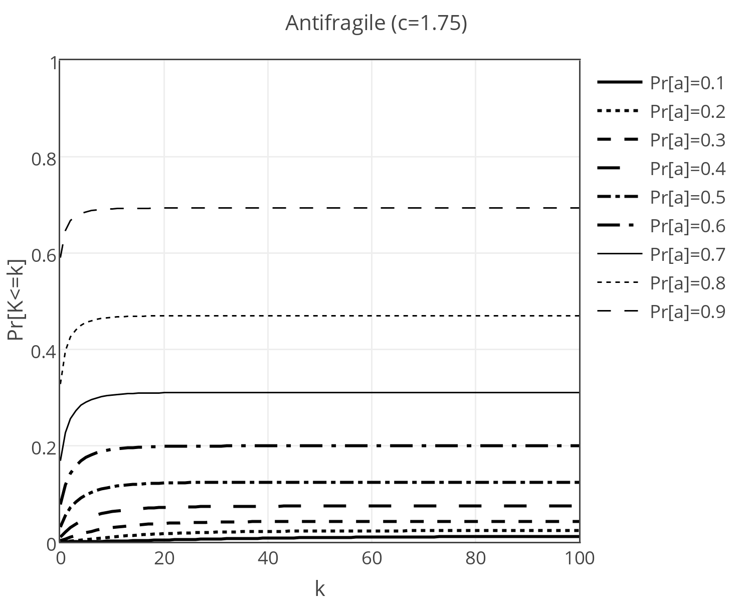
(a)

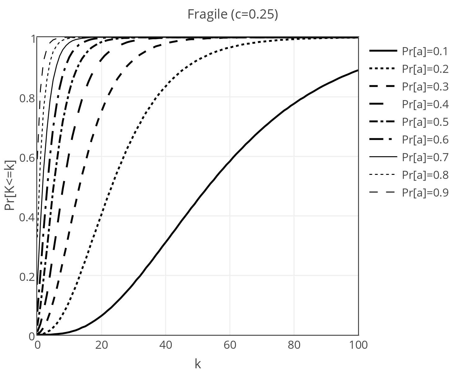
(b)

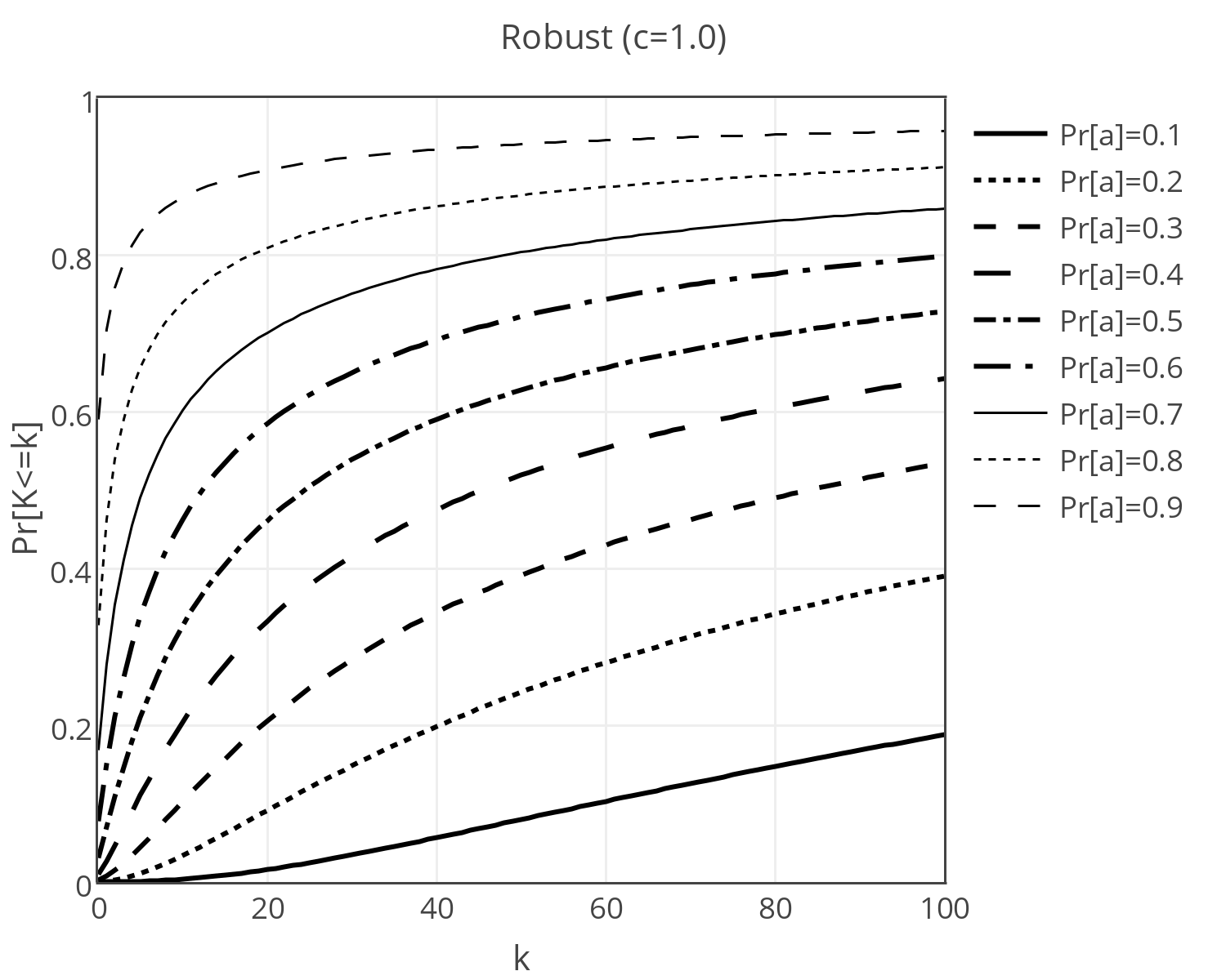
(c)

Figure 1: CDFs of several $K$s: antifragile (top left), fragile (top right), and robust (bottom), with $Pr[X_{i}=\alpha]$ from $10\%$ to $90\%$, $k$ from $0$ to $100$, $w=5$, and $w^{\prime}=1$ for each.

Because $Pr[K=k]$ represents the probability that subgroup $i$ will see exactly $k$ $\beta$s and then die off and $Pr[K<\infty]$ represents the probability that the subgroup will die off at all, the behavior of the CDF implies that an antifragile subgroup has a significant probability of “living forever,” whereas fragile subgroups have almost none and robust subgroups are not as straightforward to predict.

4 Verification

To verify the predictive power of the model, 5,000 simulations were run for each $k$ from 0 to 100 where $\beta=2$, subgroups were labeled $1..5$, subgroup $i$ was selected for growth $\frac{i}{15}$ times, and $H_{i}(0)=10$ for each subgroup. The remaining parameters are found in $(16)$ - $(24)$ such that subgroup 3 is expected to be robust, subgroups 1 and 2 are expected to be fragile, and subgroups 4 and 5 are expected to be antifragile. Figure 2 illustrates the results, comparing calculated (predicted) CDFs for each subgroup and observed (simulated) survival rates. Predictions were made in a bignumber implementation of Julia 0.3.5 and simulations were run on a 64-bit floating point implementation in Python 2.7.8.

$$\beta =\alpha^{-Pr[X_{i}=\alpha]/Pr[X_{i}=\beta]}$$ Robust (16)

$$\beta =2,Pr[X_{i}=\beta]=i/15,i=3$$ Given (17)

$$2 =\alpha^{-4}$$ (18)

$$\implies\alpha=2^{-1/4}\approx 0.84089$$ (19)

$$w =log_{\alpha}(H_{i}(0)^{-1})+1$$ Definition (20)

$$H_{i}(0) =10$$ Given (21)

$$w =log_{2^{-1/4}}(10^{-1})+1\approx 14.2877123$$ (22)

$$w^{\prime} =log_{\alpha}(\beta^{-1})$$ Definition (23)

$$w^{\prime} =log_{2^{-1/4}}(2^{-1})=4$$ (24)

Figure 2 also illustrates the behavior of a population size over time for a model configuration with 100 subgroups, $H_{i}(0)=10$ for each subgroup, $\beta=1.5$, $\alpha=0.995$, and $t\leq 200$. I compared two methods for implementing $S_{t}$: an iterative method where $S_{t}=(t\mod 51)+(\left\lfloor\frac{t}{51}\right\rfloor\mod 51)$; and a random method where $S_{t}=\text{uniform}(0,50)+\text{uniform}(0,49)$. Note the clear global convexity of the population size over time–a requirement of antifragility–, although this convexity is composed of several local periods of concavity in the iterative example. In the random examples similar patterns can be noted, although they are not as pronounced.

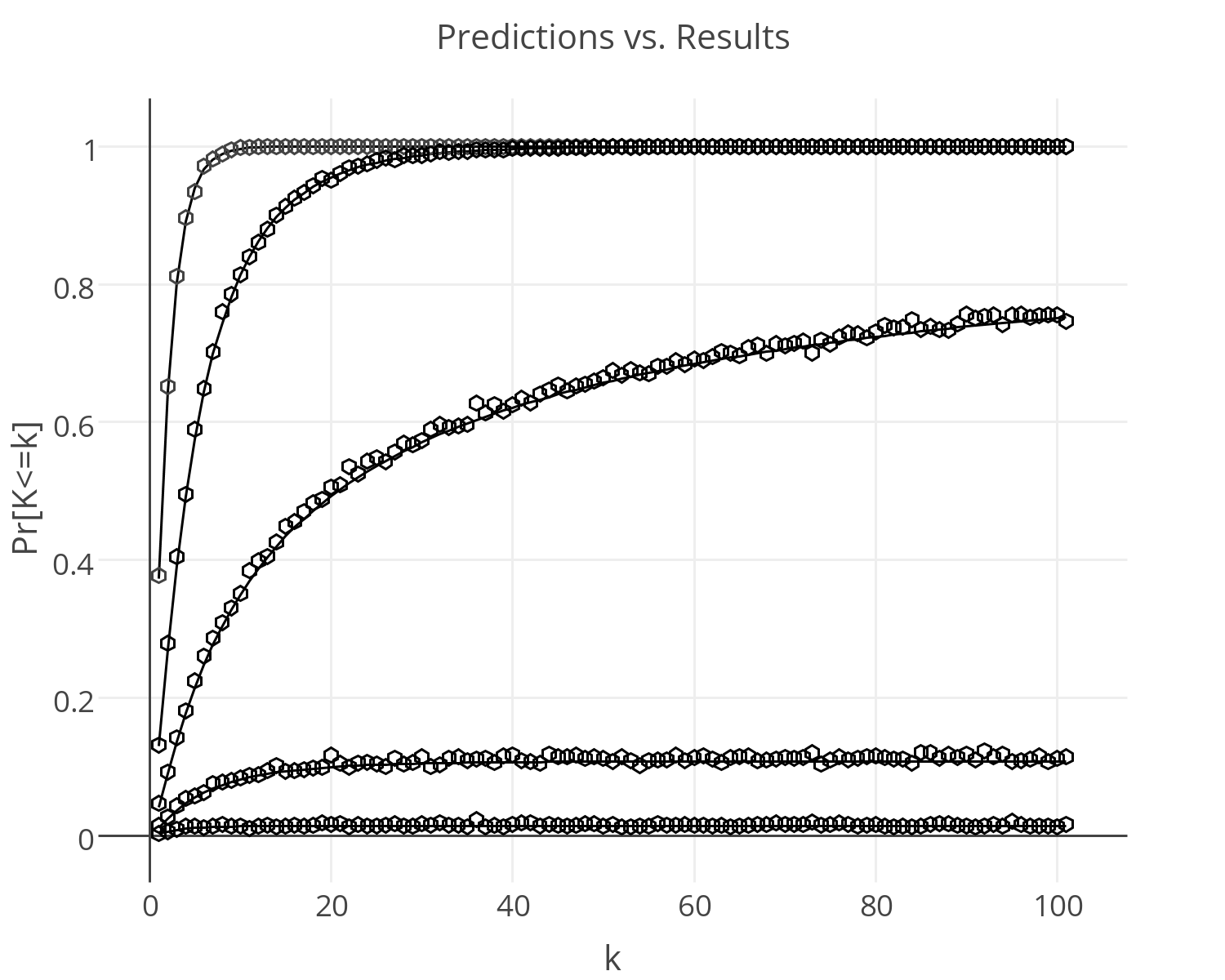
(a)

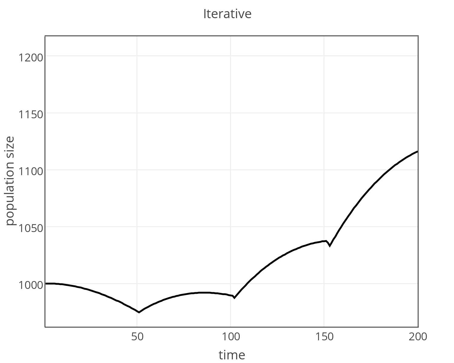
(b)

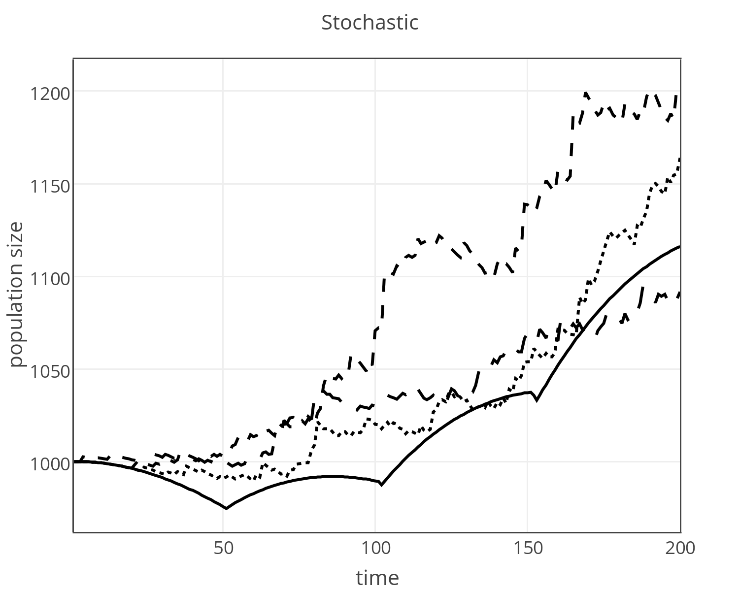
(c)

Figure 2: Comparison (top) of predicted CDFs (lines) and observed survival rates (points) for subgroups 1 (top line) through 5 (bottom line). Also, population sizes over time using an iterative method to select subgroups (bottom left) and a random method (bottom right). The iterative data is shown on the right alongside three random runs’ data for quick comparison.

5 Conclusion

I have presented and analyzed a simple model that exhibits antifragility. In this model, the population as a whole is exposed to a stressor, represented by a set of random variables. At each time step, exactly one subgroup of the population benefits from this stressor, growing in size as the others shrink. In the long run behavior of the model, the weaker (fragile) subgroups of the population die off, represented as an exponential decay function while the stronger (robust or antifragile) subgroups either maintain an approximate equilibrium or grow infinitely in size.

The model either contains no or masks with its simplicity any feedback loops, posited in [1] as necessary to produce a stable system: “positive feedback alone pushes the system beyond its limits and, eventually out of control, while negative feedback alone prevents the system from reaching its optimal behavior,” a behavior echoed here in the tendancy of fragile groups to die off, antifragile groups to grow “infinitely,” and robust groups to rest somewhere in between. Without loops of any kind, then, the proposed model is instead little more than a set of functions with tendancies to grow or decay in response to a set of random variables.

Yet does this model still suggest brute survival of the fittest? Yes, but only in cases where it is directly applicable, and these applications presuppose a static longterm stress environment and complete independence of population subgroups, neither of which are typical givens in complex systems such as social networks and biological ecosystems. This is, as it has been characterized here, the model does not support a stressor that changes suddenly, presenting an opportunity for the model to suffer the “turkey fallacy” [3], where the system is fragile to abrupt environmental changes. Furthermore, because of the aforementioned limitations on the model, a general measure of antifragility cannot be given, albeit a general sense of the term is.

However, it does demonstrate a relationship between periods of failure, represented by the decay constant $\alpha$, and periods of overcompensation, representated by the growth constant $\beta$. If an upper limit is placed on the ability of a population to overcompensate from a stressor, as one would expect is often the case in natural systems, then once that limit has been reached the population’s only choice to improve its robustness is to raise the decay factor–that is, increase $\alpha$ through some facility such that during periods of failure when overcompensation is not possible the impact of the stressor is not as severe.

References

- [1] M. Bakhouya and J. Gaber. Bio-inspired approaches for engineering adaptive systems. Procedia Computer Science, 32, 2014.
- [2] Kennie H. Jones. Engineering antifragile systems: A change in design philosophy. Procedia Computer Science, 32, 2014.
- [3] Nassim Nicholas Taleb. Antifragile: Things that gain from disorder. 2014.