An introduction to geometric complexity theory

Abstract

I survey methods from differential geometry, algebraic geometry and representation theory relevant for the permanent v. determinant problem from computer science, an algebraic analog of the ${\mathbb{P}}$ v. ${\mathbb{N}\mathbb{P}}$ problem.

1 Introduction

The purpose of this article is to introduce mathematicians to uses of geometry in complexity theory. I focus on a central question: the Geometric Complexity Theory version of L. Valiant’s conjecture comparing the complexity of the permanent and determinant polynomials, which is an algebraic variant of the ${\mathbb{P}}\neq{\mathbb{N}\mathbb{P}}$ conjecture. Other problems in complexity such as matrix rigidity (see [KLPSMN09, GHIL, Alu]) and the complexity of matrix multiplication (see, e.g., [Lan08]) have been treated with similar geometric methods.

2 History

2.1 1950’s Soviet Union

A traveling saleswoman needs to visit 20 cities; Moscow, Leningrad, Stalingrad,… Is there a route that can be taken traveling less than 10,000km?

Essentially the only known method to determine the answer is a brute force search through all possible paths. The number of paths to check grows exponentially with the number of cities to visit. Researchers in the Soviet Union asked: Is this brute force search avoidable? I.e., are there any algorithms that are significantly better than the naïve one?

A possible cause for hope is that if someone proposes a route, it is very easy to check if it is less than 10,000km (even pre-Google).

2.2 1950’s Princeton NJ

In a letter to von Neumann (see [Sip92, Appendix]) Gödel attempted to quantify the apparent difference between intuition and systematic problem solving. For example, is it really significantly easier to verify a proof than to write one?

2.3 1970’s: Precise versions of these questions

These ideas evolved to a precise conjecture posed by Cook (preceded by work of Cobham, Edmonds, Levin, Rabin, Yablonski, and the above-mentioned question of Gödel):

Let ${\mathbb{P}}$ denote the class of problems that are “easy”  to solve.

Let ${\mathbb{N}\mathbb{P}}$ denote the class of problems that are “easy”  to verify (like the traveling saleswoman problem).

Conjecture 1.

[Coo71, Kar72] ${\mathbb{P}}\neq{\mathbb{N}\mathbb{P}}$.

2.4 Late 1970’s: L. Valiant, algebraic variant

A bipartite graph is a graph with two sets of vertices and edges joining vertices from one set to the other. A perfect matching is a subset of the edges such that each vertex shares an edge from the subset with exactly one other vertex.

A standard problem in graph theory, for which the only known algorithms are exponential in the size of the graph, is to count the number of perfect matchings of a bipartite graph.

Figure 1: A bipartite graph, Vertex sets are $\{A,B,C\}$ and $\{\alpha,\beta,\gamma\}$.

Figure 2: Two perfect matchings of the graph from Figure 1.

This count can be computed by evaluating a polynomial as follows: To a bipartite graph $\Gamma$ one associates an incidence matrix $X_{\Gamma}=(x^{i}_{j})$, where $x^{i}_{j}=1$ if an edge joins the vertex $i$ above to the vertex $j$ below and is zero otherwise. For example the graph of Fig. 1 has incidence matrix

$$X_{\Gamma}=\begin{pmatrix}1&1&0\\ 0&1&1\\ 0&1&1\end{pmatrix}.$$

A perfect matching corresponds to a set of entries $\{x^{1}_{j_{1}},\ldots,x^{n}_{j_{n}}\}$ with all $x^{i}_{j_{i}}=1$ and $(j_{1},\ldots,j_{n})$ is a permutation of $(1,\ldots,n)$. Let $\mathfrak{S}_{n}$ denote the group of permutations of the elements $(1,\ldots,n)$.

Define the permanent of an $n\times n$ matrix $X=(x^{i}_{j})$ by

$$perm_{n}(X):=\sum_{\sigma\in\mathfrak{S}_{n}}x^{1}_{\sigma(1)}x^{2}_{\sigma(2)}\cdots x^{n}_{\sigma(n)}.$$ (1)

Then $\operatorname{perm}(X_{\Gamma})$ equals the number of perfect matchings of $\Gamma$.

For example, $\operatorname{perm}_{3}\begin{pmatrix}1&1&0\\ 0&1&1\\ 0&1&1\end{pmatrix}=2.$

A fast algorithm to compute the permanent would give a fast algorithm to count the number of perfect matchings of a bipartite graph.

While it may not be easy to evaluate, the polynomial $\operatorname{perm}_{n}$ is relatively easy to write down compared with a random polynomial of degree $n$ in $n^{2}$ variables in the following sense:

Let ${\mathbb{V}\mathbb{N}\mathbb{P}}$ be the set of sequences of polynomials that are “easy” to write down. Valiant showed [Val79] that the permanent is complete for the class ${\mathbb{V}\mathbb{N}\mathbb{P}}$, in the sense that ${\mathbb{V}\mathbb{N}\mathbb{P}}$ is the class of all polynomial sequences $(p_{m})$, where $p_{m}$ has degree $m$ and involves a number of variables polynomial in $m$, such that there is a polynomial $n(m)$ and $p_{m}$ is an affine linear projection of $\operatorname{perm}_{n(m)}$ as defined below. Many problems from graph theory, combinatorics, and statistical physics (partition functions) are in ${\mathbb{V}\mathbb{N}\mathbb{P}}$. A good way to think of ${\mathbb{V}\mathbb{N}\mathbb{P}}$ is as the class of sequences of polynomials that can be written down explicitly.

Let ${\mathbb{V}\mathbb{P}}$ be the set of sequences of polynomials that are “easy” to compute. For example, one can compute the determinant of an $n\times n$ matrix quickly, e.g., using Gaussian elimination, so the sequence $(\operatorname{det}_{n})\in{\mathbb{V}\mathbb{P}}$. Most problems from linear algebra (e.g., inverting a matrix, computing its determinant, multiplying matrices) are in ${\mathbb{V}\mathbb{P}}$.

The standard formula for the easy to compute determinant polynomial is

$$det_{n}(X):=\sum_{\sigma\in\mathfrak{S}_{n}}{\rm{sgn}}(\sigma)x^{1}_{\sigma(1)}x^{2}_{\sigma(2)}\cdots x^{n}_{\sigma(n)}.$$ (2)

Here ${\rm{sgn}}(\sigma)$ denotes the sign of the permutation $\sigma$.

Note that

$$\operatorname{perm}_{2}\begin{pmatrix}y^{1}_{1}&y^{1}_{2}\\ y^{2}_{1}&y^{2}_{2}\end{pmatrix} =y^{1}_{1}y^{2}_{2}+y^{1}_{2}y^{2}_{1}$$

$$=\operatorname{det}_{2}\begin{pmatrix}y^{1}_{1}&-y^{1}_{2}\\ y^{2}_{1}&y^{2}_{2}\end{pmatrix}.$$

On the other hand, Marcus and Minc [MM61], building on work of Pólya and Szegö (see [Gat87]), proved that one could not express $\operatorname{perm}_{m}(Y)$ as a size $m$ determinant of a matrix whose entries are affine linear functions of the variables $y^{i}_{j}$ when $m>2$. This raised the question that perhaps the permanent of an $m\times m$ matrix could be expressed as a slightly larger determinant. More precisely, we say $p(y^{1},\ldots,y^{M})$ is an affine linear projection of $q(x^{1},\ldots,x^{N})$, if there exist affine linear functions $x^{\alpha}(Y)=x^{\alpha}(y^{1},\ldots,y^{M})$ such that $p(Y)=q(X(Y))$. For example, B. Grenet [Gre14] observed that

$$\operatorname{perm}_{3}(Y)=\operatorname{det}_{7}\begin{pmatrix}0&y^{1}_{1}&y^{2}_{1}&y^{3}_{1}&0&0&0\\ 0&1&0&0&y^{3}_{3}&y^{2}_{3}&0\\ 0&0&1&0&0&y^{1}_{3}&y^{3}_{3}\\ 0&0&0&1&y^{1}_{3}&0&y^{2}_{3}\\ y^{2}_{2}&0&0&0&1&0&0\\ y^{3}_{2}&0&0&0&0&1&0\\ y^{1}_{2}&0&0&0&0&0&1\end{pmatrix}.$$ (3)

Recently [ABV15] it was shown that $\operatorname{perm}_{3}$ cannot be realized as an affine linear projection of $\operatorname{det}_{n}$ for $n\leq 6$, so (3) is optimal.

Valiant showed that if $n(m)$ grows exponentially with respect to $m$, then there exist affine linear functions $x^{i}_{j}(y^{s}_{t})$ such that $\operatorname{det}_{n}(X(Y))=\operatorname{perm}_{m}(Y)$. (Grenet strengthened this to show explicit expressions when $n=2^{m}-1$ [Gre14]. See [LR15] for a discussion of the geometry of these algorithms and a proof of their optimality among algorithms with symmetry.) Valiant also conjectured that one cannot do too much better:

Conjecture 2 (Valiant [Val79]).

Let $n(m)$ be a polynomial of $m$. Then there exists an $m_{0}$ such that for all $m>m_{0}$, there do not exist affine linear functions $x^{i}_{j}(y^{s}_{t})$ such that $\operatorname{perm}_{m}(Y)=\operatorname{det}_{n}(X(Y))$.

Remark 3.

The original ${\mathbb{P}}\neq{\mathbb{N}\mathbb{P}}$ is viewed as completely out of reach. Conjecture 2, which would be implied by ${\mathbb{P}}\neq{\mathbb{N}\mathbb{P}}$ is viewed as a more tractable substitute.

To keep track of progress on the conjecture, for a polynomial $p=p(Y)$, let $dc(p)$ denote the smallest $n$ such that there exists an affine linear map $X(Y)$ satisfying $p(Y)=\operatorname{det}_{n}(X(Y))$. Then Conjecture 2 says that $dc(\operatorname{perm}_{m})$ grows faster than any polynomial. Since the conjecture is expected to be quite difficult, one could try to prove any lower bound on $dc(\operatorname{perm}_{m})$. Several linear bounds on $dc(\operatorname{perm}_{m})$ were shown [MM61, vzG87, Cai90] with the current world record the quadratic bound $dc(\operatorname{perm}_{m})\geq\frac{m^{2}}{2}$ [MR04]. (Over finite fields one has the same bound by [Cai90]. Over $\mathbb{R}$, one has $dc_{\mathbb{R}}(\operatorname{perm}_{m})\geq m^{2}-2m+2$ [Yab15].) The state of the art was obtained with local differential geometry, as described in §3.

Remark 4.

There is nothing special about the permanent for this conjecture: it would be sufficient to show any explicit (in the sense of ${\mathbb{V}\mathbb{N}\mathbb{P}}$ mentioned above) sequence of polynomials $p_{m}$ has $dc(p_{m})$ growing faster than any polynomial. The dimension of the set of affine linear projections of $\operatorname{det}_{n}$ is roughly $n^{4}$, but the dimension of the space of homogeneous polynomials of degree $m$ in $m^{2}$ variables grows almost like $m^{m}$, so a random sequence will have exponential $dc(p_{m})$. Problems in computer science to find an explicit object satisfying a property that a random one satisfies are called trying to find hay in a haystack.

2.5 Coordinate free version

To facilitate the use of geometry, we get rid of coordinates. Let $\operatorname{End}(\mathbb{C}^{n^{2}})$ denote the space of linear maps $\mathbb{C}^{n^{2}}\rightarrow\mathbb{C}^{n^{2}}$, which acts on the space of homogeneous polynomials of degree $n$ on $\mathbb{C}^{n^{2}}$, denoted $S^{n}\mathbb{C}^{n^{2}*}$ (where the $*$ is used to indicate the dual vector space to $\mathbb{C}^{n^{2}}$), as follows: for $g\in\operatorname{End}(\mathbb{C}^{n^{2}})$ and $P\in S^{n}\mathbb{C}^{n^{2}*}$, the polynomial $g\cdot P$ is defined by

$$(g\cdot P)(x):=P(g^{T}x).$$ (4)

Here $g^{T}$ denotes the transpose of $g$. (One takes the transpose matrix in order that $g_{1}\cdot(g_{2}\cdot P)=(g_{1}g_{2})\cdot P$.)

In [MS01] they introduced padding; adding a homogenizing variable so all objects live in the same ambient space, in order to deal with linear functions instead of affine linear functions. Let $\ell$ be a new variable, so $\ell^{n-m}\operatorname{perm}_{m}(y)\in S^{n}\mathbb{C}^{(m^{2}+1)*}$. Then $\operatorname{perm}_{m}(y)$ is expressible as an $n\times n$ determinant whose entries are affine linear combinations of the $y^{i}_{j}$ if and only if $\ell^{n-m}\operatorname{perm}_{m}$ is expressible as an $n\times n$ determinant whose entries are linear combinations of the variables $y^{i}_{j},\ell$.

Consider any linear inclusion $\mathbb{C}^{(m^{2}+1)*}\rightarrow\mathbb{C}^{n^{2}*}$, so in particular $\ell^{n-m}\operatorname{perm}_{m}\in S^{n}\mathbb{C}^{n^{2}*}$. Then

$$dc(\operatorname{perm}_{m})\leq n\Leftrightarrow\ell^{n-m}\operatorname{perm}_{m}\in\operatorname{End}(\mathbb{C}^{n^{2}})\cdot\operatorname{det}_{n}.$$ (5)

Conjecture 2 in this language is:

Conjecture 5 (Valiant [Val79]).

Let $n(m)$ be a polynomial of $m$. Then there exists an $m_{0}$ such that for all $m>m_{0}$, $\ell^{n-m}\operatorname{perm}_{m}\not\in\operatorname{End}(\mathbb{C}^{n^{2}})\cdot\operatorname{det}_{n}$, equivalently

$$\operatorname{End}(\mathbb{C}^{n^{2}})\cdot\ell^{n-m}\operatorname{perm}_{m}\not\subset\operatorname{End}(\mathbb{C}^{n^{2}})\cdot\operatorname{det}_{n}.$$

3 Differential geometry and the state of the art regarding Conjecture 2

The best result pertaining to Conjecture 2 comes from local differential geometry: the study of Gauss maps.

3.1 Gauss maps

Given a surface in $3$-space, form its Gauss map by mapping a point of the surface to its unit normal vector on the unit sphere as in Figure 3.

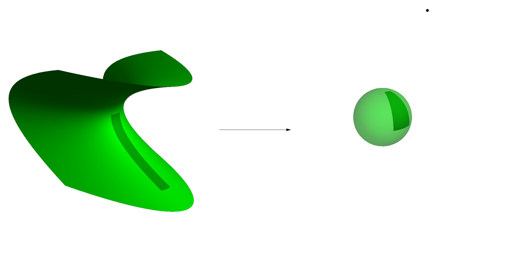
Figure 3: The shaded area of the surface maps to the shaded area of the sphere.

A normal vector to a surface $X$ at $x$ is one perpendicular to the tangent space $T_{x}X\subset\mathbb{R}^{3}$. This Gauss image can be defined without the use of an inner product if one instead takes the union of all conormal lines, where a conormal vector to $X\subset\mathbb{R}^{3}$ is one in the dual space $\mathbb{R}^{3*}$ that annhilates the tangent space $T_{x}X$. One loses qualitiative information, however one still has the information of the dimension of the Gauss image.

This dimension will drop if through all points of the surface there is a curve along which the tangent plane is constant. For example, if $M$ is a cylinder, i.e., the union of lines in three space perpendicular to a plane curve, the Gauss image is a curve:

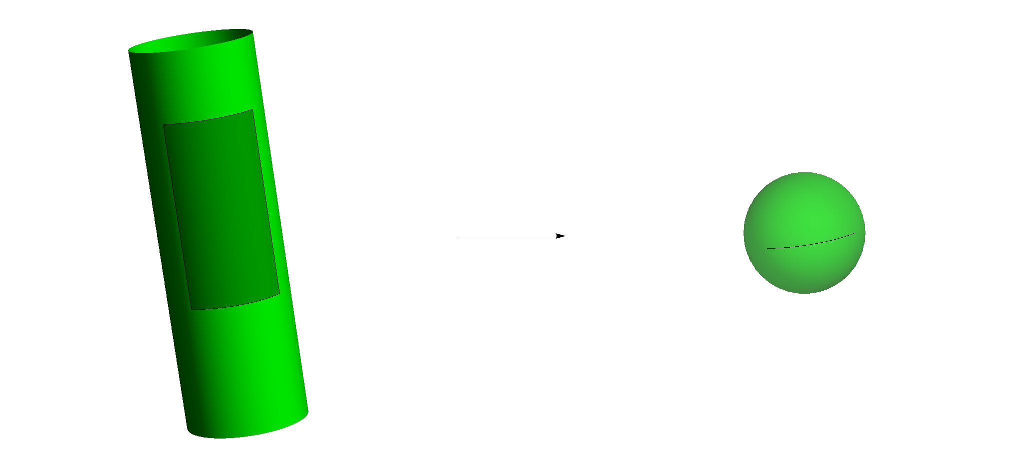
Figure 4: Lines on the cylinder are collapsed to a point.

The extreme case is when the surface is a plane, then its Gauss image is just a point.

A classical theorem in the geometry of surfaces in three-space classifies surfaces with degenerate Gauss image. I state it in the algebraic category for what comes next (for $C^{\infty}$ versions see, e.g., [Spi79, vol. III, chap. 5]). One may view projective space $\mathbb{P}^{3}$ as affine space with a plane added at infinity. From this perspective a cylinder is a cone with vertex at infinity.

Theorem 6 (C. Segre [Seg10]).

If $X^{2}\subset\mathbb{P}^{3}$ is an algebraic surface whose Gauss image is not two-dimensional, then $X$ is one of:

• The closure of the union of points on tangent lines to a space curve.

• A generalized cone, i.e., the points on the union of lines connecting a fixed point to a plane curve.

Notice that in the first picture, the tangent plane along a ray of the curve is constant, and in the second case the tangent plane is constant along the lines through the vertex.

One can extend the notion of Gauss map to hypersurfaces of arbitrary dimension, and to hypersurfaces defined over the complex numbers. The union of tangent rays to a curve generalizes to the case of osculating varieties. One can also take cones with vertices larger than a point.

3.2 What does this have to do with complexity theory?

The hypersurface $\{\operatorname{det}_{n}(X)=0\}\subset\mathbb{C}^{n^{2}}$ has a very degenerate Gauss map. To see this, consider the matrix

$$z=\begin{pmatrix}1&&&\\ &\ddots&&\\ &&1&\\ &&&0\end{pmatrix}\in\{\operatorname{det}_{n}=0\}.$$

The tangent space to $\{\operatorname{det}_{n}=0\}$ at $z$, and the conormal space (in the dual space of matrices) are respectively

$$T_{z}\{\operatorname{det}_{n}=0\}=\begin{pmatrix}*&*&*&*\\ \vdots&\ddots&\vdots&\vdots\\ *&*&*&*\\ *&*&*&0\end{pmatrix},\ \ \ \ \ \ \ N^{*}_{z}\{\operatorname{det}_{n}=0\}=\begin{pmatrix}0&0&0&0\\ \vdots&\ddots&\vdots&\vdots\\ 0&0&0&0\\ 0&0&0&*\end{pmatrix}.$$

But any rank $n-1$ matrix whose non-zero entries all lie in the upper left $(n-1)\times(n-1)$ submatrix will have the same tangent space! Since any smooth point of $\{\operatorname{det}_{n}=0\}$ can be moved to $z$ by a change of basis, we conclude that the tangent hyperplanes to $\{\operatorname{det}_{n}=0\}$ are parametrized by the rank one matrices, the space of which has dimension $2n-1$ (or $2n-2$ in projective space), because they are obtained by multiplying a column vector by a row vector. In fact, $\{\operatorname{det}_{n}=0\}$ may be thought of as an osculating variety of the variety of rank one matrices (e.g., the union of tangent lines to the union of tangent lines… to the variety of rank one matrices).

On the other hand, a direct calculation shows that the permanent hypersurface $\{\operatorname{perm}_{m}=0\}\subset\mathbb{P}^{m^{2}-1}$ has a non-degenerate Gauss map (see §5.3), so when one includes $\mathbb{C}^{m^{2}}\subset\mathbb{C}^{n^{2}}$, the equation $\{\operatorname{perm}_{m}=0\}$ becomes an equation in a space of $n^{2}$ variables that only uses $m^{2}$ of the variables, one gets a cone with vertex $\mathbb{P}^{n^{2}-m^{2}-1}$ corresponding to the unused variables, in particular, the Gauss image will have dimension $m^{2}-2$.

If one makes an affine linear substitution $X=X(Y)$, the Gauss map of $\{\operatorname{det}(X(Y))=0\}$ will be at least as degenerate as the Gauss map of $\{\operatorname{det}(X)=0\}$. Using this, one obtains:

Theorem 7 (Mignon-Ressayre [MR04]).

If $n(m)<\frac{m^{2}}{2}$, then there do not exist affine linear functions $x^{i}_{j}(y^{s}_{t})$ such that $\operatorname{perm}_{m}(Y)=\operatorname{det}_{n}(X(Y))$. I.e., $dc(\operatorname{perm}_{m})\geq\frac{m^{2}}{2}$.

4 Algebraic geometry and Valiant’s conjecture

A possible path to show $\operatorname{perm}_{m}(Y)\neq\operatorname{det}_{n}(X(Y))$ is to look for a polynomial whose zero set contains all polynomials of the form $\operatorname{det}_{n}(X(Y))$, and show that $\operatorname{perm}_{m}$ is not in the zero set.

4.1 Polynomials

Algebraic geometry is the study of zero sets of polynomials. In our situation, we need polynomials on spaces of polynomials. More precisely, if

$$P(x_{1},\ldots,x_{N})=\sum_{1\leq i_{1}\leq\cdots\leq i_{d}\leq N}c_{i_{1},\ldots,i_{d}}x_{i_{1}}\cdots x_{i_{d}}$$

is a homogeneous polynomial of degree $d$ in $N$ variables, we work with polynomials in the coefficients $c_{i_{1},\ldots,i_{d}}$, where these coefficients provide coordinates on the vector space $S^{d}\mathbb{C}^{N}$ of all homogeneous polynomials of degree $d$ in $N$ variables.

The starting point of Geometric Complexity Theory is the plan to prove Valiant’s conjecture by finding a sequence of polynomials $P_{m}$ vanishing on all affine-linear projections of $\operatorname{det}_{n(m)}$ when $n$ is a polynomial in $m$ such that $P_{m}$ does not vanish on $\operatorname{perm}_{m}$.

4.2 Disadvantage of algebraic geometry?

The zero set of all polynomials vanishing on

$$S:=\{(z,w)\mid w=0,\ z\neq 0\}\subset\mathbb{C}^{2},$$

is the line

$$\{(z,w)\mid w=0\}\subset\mathbb{C}^{2}.$$

That is, if we want to use polynomials, we may need to prove a more difficult conjecture, in the sense that we will need to prove non-membership in a larger set.

Given a subset $Z$ of a vector space $U$, the ideal of $Z$, denoted $I(Z)$, is the set of all polynomials vanishing at all points of $Z$. The Zariski closure of $Z$, denoted $\overline{Z}$, is the set of $u\in U$ such that $P(u)=0$ for all $P\in I(Z)$. The common zero set of a collection of polynomials (such as $\overline{Z}$) is called an algebraic variety.

Conjecture 8 (Mulmuley-Sohoni [MS01]).

Let $n(m)$ be a polynomial of $m$. Then there exists an $m_{0}$ such that for all $m>m_{0}$, $\ell^{n-m}\operatorname{perm}_{m}\not\in\overline{\operatorname{End}(\mathbb{C}^{n^{2}})\cdot\operatorname{det}_{n}}$.

How serious a problem is the issue of Zariski closure? Does it really change Valiant’s conjecture?

Mulmuley conjectures [MN] that indeed it does. Namely, he conjectures that there are sequences in the closure of the sequences of spaces $\operatorname{End}(\mathbb{C}^{n^{2}})\cdot\operatorname{det}_{n}$ that are not in ${\mathbb{V}\mathbb{P}}$.

Example 9.

Let $P=x_{1}^{3}+x_{2}^{2}x_{3}+x_{2}x_{4}^{2}\in S^{3}\mathbb{C}^{4}$. Then $P\not\in\operatorname{End}(\mathbb{C}^{n^{2}})\cdot\operatorname{det}_{n}$ for $n<5$ [ABV15]. However, $\overline{\operatorname{End}(\mathbb{C}^{9})\cdot\operatorname{det}_{3}}\supset S^{3}\mathbb{C}^{4}$, i.e., every homogeneous polynomial of degree $3$ in $4$ variables is in the Zariski closure of degenerations of $\operatorname{det}_{3}$, see e.g., [Bea00].

However, Mulmuley also conjectures [MN] that any path to resolving Valiant’s conjecture will have to address “wild” sequences in the closure, so that the stronger conjecture is the more natural one. Moreover Grochow makes the case [Joshunify] that essentially all lower bounds in algebraic complexity theory have come from algebraic geometry.

4.3 Advantage of the stronger conjecture: representation theory

Representation theory is the systematic study of symmetry in linear algebra.

The variety $\overline{\operatorname{End}(\mathbb{C}^{n^{2}})\cdot\operatorname{det}_{n}}$ may be realized as an orbit closure as follows: Let $GL_{N}$ denote the group of invertible $N\times N$ matrices. It acts on the space of polynomials $S^{d}\mathbb{C}^{N}$ by (4). Any element of $\operatorname{End}(\mathbb{C}^{N})$ my be described as a limit of elements of $GL_{N}$, so the Euclidean closure of $\operatorname{End}(\mathbb{C}^{N})\cdot\operatorname{det}_{n}$ equals the Euclidean closure of $GL_{N}\cdot\operatorname{det}_{n}$. In general Euclidean and Zariski closure can be quite different (e.g. the Zariski closure of $\{(z,w)\mid z=0,\ w\in\mathbb{Z}\}\subset\mathbb{C}^{2}$ is the line but this set is already Euclidean closed). However, in this situation Euclidean closure equals Zariski closure (see [Mum95, Thm. 2.33]), so we have the following equality of Zariski closures:

$$\overline{GL_{n^{2}}\cdot\operatorname{det}_{n}}=\overline{\operatorname{End}(\mathbb{C}^{n^{2}})\cdot\operatorname{det}_{n}}.$$

Substantial techniques have been developed to study orbits and their closures.

Let

$${\mathcal{\hat{D}}et}_{n}:=\overline{GL_{n^{2}}\cdot\operatorname{det}_{n}}$$

and let

$${\mathcal{\hat{P}}erm}^{m}_{n}:=\overline{GL_{n^{2}}\cdot\ell^{n-m}\operatorname{perm}_{m}}.$$

Conjecture 10.

[MS01] Let $n=m^{c}$ for any constant $c$. Then for all sufficiently large $m$,

$${\mathcal{\hat{P}}erm}^{m}_{n}\not\subset{\mathcal{\hat{D}}et}_{n}.$$

Conjecture 10 would imply Conjecture 2. In §7, I describe the program to use representation theory to prove Conjecture 10.

5 State of the art for conjecture 10: classical algebraic geometry

5.1 Classical algebraic geometry detour: B. Segre’s dimension formula

In algebraic geometry it is more convenient to work in projective space. (From a complexity perspective it is also natural, as changing a function by a scalar will not change its complexity.) If $W$ is a vector space then $\mathbb{P}W$ is the associated projective space of lines through the origin: $\mathbb{P}W=(W\backslash 0)/\sim$ where $w_{1}\sim w_{2}$ if $w_{1}=\lambda w_{2}$ for some nonzero complex number $\lambda$. Write $[w]\in\mathbb{P}W$ for the equivalence class of $w\in W\backslash 0$ and if $X\subset\mathbb{P}W$, let $\hat{X}\subset W$ denote the corresponding cone in $W$. Define $\overline{X}=\pi(\overline{\hat{X}})$, the Zariski closure of $X$.

If $X\subset\mathbb{P}W$ is a hypersurface, let $X{{}^{\vee}}\subset\mathbb{P}W^{*}$ denote its Gauss image, which is called its dual variety. If $X$ is an irreducible algebraic variety, $X{{}^{\vee}}$ will be too. More precisely, $X{{}^{\vee}}$ is the Zariski closure of the set of conormal lines to smooth points of $X$. Here, if $\hat{T}_{x}X\subset W$ denotes the tangent space to the cone over $X$, the conormal space is $N^{*}_{x}X=(\hat{T}_{x}X){}^{\perp}\subset W^{*}$.

Proposition 11 (B. Segre [Seg51]).

Let $P\in S^{d}W^{*}$ be irreducible and let $d\geq 2$. Then for a Zariski open subset of points $[x]\in{\rm Zeros}(P)$,

$${\rm dim}\;{\rm Zeros}(P){{}^{\vee}}={\mathrm{rank}}(Hess(P)(x^{d-2}))-2.$$

Here $(Hess(P)(x^{d-2}))\in S^{2}W^{*}$ is the Hessian matrix of second partial derivatives of $P$ evaluated at $x$. Note that the right hand side involves second derivative information, and the left hand side involves the dual variety (which is first derivative information from ${\rm Zeros}(P)$), and its dimension, which is a first derivative computation on the dual variety, and therefore a second derivative computation on ${\rm Zeros}(P)$.

Proof.

For a homogeneous polynomial $P\in S^{d}W^{*}$, write $\overline{P}$ when we consider $P$ as a $d$-multi-linear form. Let $x\in{{\hat{Z}}eros}(P)\subset W$ be a smooth point, so $P(x)=\overline{P}(x,\ldots,x)=0$ and $dP_{x}=\overline{P}(x,\ldots,x,\cdot)\neq 0$. Take $h=dP_{x}\in W^{*}$, so $[h]\in{\rm Zeros}(P){{}^{\vee}}$. Consider a curve $h_{t}\subset{{\hat{Z}}eros}(P){{}^{\vee}}$ with $h_{0}=h$. There must be a corresponding curve $x_{t}\in{{\hat{Z}}eros}(P)$ such that $h_{t}=\overline{P}(x_{t},\ldots,x_{t},\cdot)$ and thus its derivative is $h_{0}^{\prime}=\overline{P}(x^{d-2},x_{0}^{\prime},\cdot)$. The dimension of $\hat{T}_{h}{\rm Zeros}(P){{}^{\vee}}$ is then the rank of $Hess(P)(x^{d-2})=\overline{P}(x^{d-2},\cdot,\cdot)$ minus one (we subtract one because $x_{0}^{\prime}=x$ is in the kernel of $Hess(P)(x^{d-2})$). Finally $\operatorname{dim}X=\operatorname{dim}\hat{T}_{x}X-1$. ∎

5.2 First steps towards equations

Segre’s formula implies, for $P\in S^{d}W^{*}$, that $\operatorname{dim}{\rm Zeros}(P){{}^{\vee}}\leq k$ if and only if, for all $w\in W$, letting $G(q,W)$ denote the Grassmannian of $q$-planes through the origin in $W$,

$$P(w)=0\ \ \Rrightarrow\ \ \operatorname{det}_{k+3}(Hess(P)(w^{d-2})|_{F})=0\ \forall F\in G(k+3,W).$$

Equivalently (assuming $P$ is irreducible), for any $F\in G(k+3,W)$, the polynomial $P$ must divide $\det_{k+3}(Hess(P)|_{F})\in S^{(k+3)(d-2)}W^{*}$.

Thus to find polynomials on $S^{d}W^{*}$ characterizing hypersurfaces with degenerate duals, we need polynomials that detect if a polynomial $P\in S^{d}W^{*}$ divides a polynomial $Q\in S^{e}W^{*}$. Now $P$ divides $Q$ if and only if $Q\in P\cdot S^{e-d}W^{*}$, i.e., letting $x^{I_{j}}$ be a basis of $S^{e-d}W^{*}$ and let $\wedge$ denote exterior (wedge) product,

$$x^{I_{1}}P\wedge\cdots\wedge x^{I_{D}}P\wedge Q=0.$$ (6)

Let $\operatorname{dim}W=N$ and let ${\mathcal{D}}_{k,d,N}\subset\mathbb{P}S^{d}W^{*}$ denote the zero set of the equations (6) in the coefficients of $P$ taking $Q=\det_{k+3}(Hess(P)|_{F})$. By our previous discussion $[\operatorname{det}_{n}]\in{\mathcal{D}}_{2n-2,n,n^{2}}$.

5.3 The lower bound on $\overline{dc}(\operatorname{perm}_{m})$

When

$$x=\begin{pmatrix}1-m&1&\cdots&1\\ 1&1&\cdots&1\\ \vdots&\vdots&\cdots&\vdots\\ 1&1&\cdots&1\end{pmatrix},$$ (7)

a short calculation shows that $Hess(\operatorname{perm}_{m})(x^{m-2})$ is of maximal rank. This fills in the missing step of the proof of Theorem 7. Moreover, if one works over $\mathbb{R}$, then the Hessian has a signature. For $\operatorname{det}_{n}$, this signature is $(n-1,n-1)$, but for the permanent the signature on an open subset is at least $(m^{2}-2m+1,2m-3)$, thus:

Theorem 12 (Yabe [Yab15]).

$dc_{\mathbb{R}}(\operatorname{perm}_{m})\geq m^{2}-2m+2$.

Were we to just consider $\operatorname{perm}_{m}$ as a polynomial in more variables, the rank of the Hessian would not change. However, we are also adding padding, which could a priori have a negative effect on the rank of the Hessian. Fortunately, as was shown in [LMR13] it does not, and we conclude:

Theorem 13.

[LMR13] ${\mathcal{P}erm}^{m}_{n}\not\subset{\mathcal{D}}_{2n-2,n,n^{2}}$ when $m<\frac{n^{2}}{2}$. In particular, when $m<\frac{n^{2}}{2}$, ${\mathcal{P}erm}^{m}_{n}\not\subset{\mathcal{D}et}_{n}$.

On the other hand, since cones have degenerate duals, $\ell^{n-m}\operatorname{perm}_{m}\in{\mathcal{D}}_{2n-2,n,n^{2}}$ whenever $m\geq\frac{n^{2}}{2}$.

In [LMR13] it was also shown that ${\mathcal{D}}_{k,d,N}$ intersected with the set of irreducible hypersurfaces is exactly the set (in $\mathbb{P}S^{d}W^{*}$) of irreducible hypersurfaces of degree $d$ in $\mathbb{P}W$ with dual varieties of dimension $k$, which solved a classical question in algebraic geometry.

6 Necessary conditions for modules of polynomials to be useful for GCT

Fixing a linear inclusion $\mathbb{C}^{m^{2}+1}\subset\mathbb{C}^{n^{2}}$, the polynomial $\ell^{n-m}\operatorname{perm}_{m}\in S^{n}\mathbb{C}^{n^{2}}$ has evident pathologies: it is padded, that is divisible by a large power of a linear form, and its zero set is a cone with a $n^{2}-m^{2}-1$ dimensional vertex, that is, it only uses $m^{2}+1$ of the $n^{2}$ variables in an expression in good coordinates. To separate $\ell^{n-m}\operatorname{perm}_{m}$ from $\operatorname{det}_{n}$, one must look for modules in $I({\mathcal{D}et}_{n})$ that do not vanish automatically on equations of hypersurfaces with these pathologies. It is easy to determine such modules with representation theory. Before doing so, I first review the irreducible representations of the general linear group.

6.1 $GL(V)$-modules

Let $V$ be a complex vector space of dimension $\mathbb{v}$. The irreducible representations of $GL(V)$ are indexed by sequences of integers $\pi=(p_{1},\ldots,p_{\mathbb{v}})$ with $p_{1}\geq\cdots\geq p_{\mathbb{v}}$ and the corresponding module is denoted $S_{\pi}V$. The representations occurring in the tensor algebra of $V$ are those with $p_{\mathbb{v}}\geq 0$, i.e., by partitions. For a partition $\pi$, let $\ell(\pi)$ denote its length, the smallest $s$ such that $p_{s+1}=0$. In particular $S_{(d)}V=S^{d}V$, and $S_{(1,\ldots,1)}=:S_{(1^{d})}V=\Lambda^{d}V\subset V^{{\mathord{\otimes}}d}$, the skew-symmetric tensors.

One way to construct $S_{\pi}V$, where $\pi=(p_{1},\ldots,p_{\mathbb{v}})$ and its conjugate partition is $\pi^{\prime}=(q_{1},\ldots,q_{p_{1}})$, is to form a projection operator from $V^{{\mathord{\otimes}}|\pi|}$ by first projecting to $\Lambda^{q_{1}}V{\mathord{\otimes\cdots\otimes}\;}\Lambda^{q_{p_{1}}}V$ by skew-symmetrizing and then re-ordering and projecting the image to $S^{p_{1}}V{\mathord{\otimes\cdots\otimes}\;}S^{p_{\mathbb{v}}}V$. In particular if an element of $V^{{\mathord{\otimes}}|\pi|}$ lies in some $W^{{\mathord{\otimes}}|\pi|}$ for some $W\subset V$ with $\operatorname{dim}W<q_{1}$, then it will map to zero.

6.2 Polynomials useful for GCT

To be useful for GCT, a module of polynomials should not vanish identically on cones or on polynomials that are divisible by a large power of a linear form. The equations for the variety of polynomials whose zero sets are cones are well known – they are all modules where the length of the partition is longer than the number of variables needed to define the polynomial.

Proposition 14.

[KL14] Necessary conditions for a module $S_{{\pi}}\mathbb{C}^{n^{2}}\subset I_{d}({\mathcal{D}et}_{n})$ to not vanish identically on polynomials in $m^{2}$ variables padded by $\ell^{n-m}$ are

1. $\ell(\pi)\leq m^{2}+1$,

2. If $\pi=(p_{1},\ldots,p_{t})$, then $p_{1}\geq d(n-m)$.

Moreover, if $p_{1}\geq\operatorname{min}\{d(n-1),dn-m\}$, then the necessary conditions are also sufficient. In particular, for $p_{1}$ sufficiently large, these conditions depend only on the partition $\pi$, not how the module $S_{\pi}\mathbb{C}^{n^{2}}$ is realized as a space of polynomials.

7 The program to find modules in $I[{\mathcal{D}et}_{n}]$ via representation theory

In this section I present the program initiated in [MS01] and developed in [BLMW11, MS08] to find modules in the ideal of ${\mathcal{D}et}_{n}$.

7.1 Preliminaries

Let $W=\mathbb{C}^{n^{2}}$ and consider $\operatorname{det}_{n}\in S^{n}W^{*}$. Define $\mathbb{C}[{\mathcal{D}et}_{n}]:=Sym(S^{n}W)/I({\mathcal{D}et}_{n})$, the homogeneous coordinate ring of ${\mathcal{\hat{D}}et}_{n}$. This is the space of polynomial functions on ${\mathcal{\hat{D}}et}_{n}$ inherited from polynomials on the ambient space $S^{n}W$.

Since $Sym(S^{n}W)$ and $I({\mathcal{D}et}_{n})$ are $GL(W)$-modules, so is $\mathbb{C}[{\mathcal{D}et}_{n}]$, and since $GL(W)$ is reductive (a complex algebraic group $G$ is reductive if $U\subset V$ is a $G$-submodule of a $G$-module $V$, there exists a complementary $G$-submodule $U^{c}$ such that $V=U\oplus U^{c}$) we obtain the splitting as a $GL(W)$-module:

$$Sym(S^{n}W)=I({\mathcal{D}et}_{n})\oplus\mathbb{C}[{\mathcal{D}et}_{n}].$$

In particular, if a module $S_{\pi}W$ appears in $Sym(S^{n}W)$ and it does not appear in $\mathbb{C}[{\mathcal{D}et}_{n}]$, it must appear in $I({\mathcal{D}et}_{n})$.

For those not familiar with the ring of regular functions on an affine algebraic variety, consider $GL(W)\subset\mathbb{C}^{n^{2}+1}$ as the subvariety of $\mathbb{C}^{n^{2}+1}$, with coordinates $(x^{i}_{j},t)$ given by the equation $t\operatorname{det}(x)=1$, and $\mathbb{C}[GL(W)]$ can be defined to be the restriction of polynomial functions on $\mathbb{C}^{n^{2}+1}$ to this subvariety. Then $\mathbb{C}[GL(W)\cdot\operatorname{det}_{n}]=\mathbb{C}[GL(W)/G_{\operatorname{det}_{n}}]$ can be defined as the subring of $G_{\operatorname{det}_{n}}$-invariant functions $\mathbb{C}[GL(W)]^{G_{\operatorname{det}_{n}}}$. Here $G_{\operatorname{det}_{n}}:=\{g\in GL(W)\mid g\cdot\operatorname{det}_{n}=\operatorname{det}_{n}\}\simeq SL_{n}\times SL_{n}\ltimes\mathbb{Z}_{2}$. A nice proof of this result (originally due to Frobenius [Fro97]) is due to Dieudonné [Die49] (see [Lan15] for an exposition). It relies on the fact that, in analogy with a smooth quadric hypersurface, there are two families of maximal linear spaces on the Grassmannian $G(n^{2}-n,\mathbb{C}^{n}{\mathord{\otimes}}\mathbb{C}^{n})$ with prescribed dimensions of their intersections. One then uses that the group action must preserve these intersection properties.

There is an injective map

$$\mathbb{C}[{\mathcal{D}et}_{n}]\rightarrow\mathbb{C}[GL(W)\cdot\operatorname{det}_{n}]$$

given by restriction of functions. The map is an injection because any function identically zero on a Zariski open subset of an irreducible variety is identically zero on the variety. The algebraic Peter-Weyl theorem below gives a description of the $G$-module structure of $\mathbb{C}[G/H]$ when $G$ is a reductive algebraic group and $H$ is a subgroup.

Plan of [MS01, MS08]: Find a module $S_{\pi}W$ not appearing in $\mathbb{C}[GL(W)/G_{\operatorname{det}_{n}}]$ that does appear in $Sym(S^{n}W)$.

By the above discussion such a module must appear in $I({\mathcal{D}et}_{n})$.

One might object that the coordinate rings of different orbits could coincide, or at least be very close. Indeed this is the case for generic polynomials, but in GCT one generally restricts to polynomials whose symmetry groups are not only “large”, but they characterize the orbit as follows:

Definition 15.

Let $V$ be a $G$-module. A point $P\in V$ is characterized by its stabilizer $G_{P}$ if any $Q\in V$ with $G_{Q}\supseteq G_{P}$ is of the form $Q=cP$ for some constant $c$.

One can think of polynomial sequences that are complete for their complexity classes and are characterized by their stabilizers as “best”  representatives of their class. Corollary 17 will imply that if $P\in S^{d}V$ is characterized by its stabilizer, the coordinate ring of its $G$-orbit is unique as a module among orbits of points in $V$.

7.2 The algebraic Peter-Weyl theorem

Let $G$ be a complex reductive algebraic group (e.g. $G=GL(W)$), and let $V$ be an irreducible $G$-module. Given $v\in V$ and $\alpha\in V^{*}$, define a function $f_{v,\alpha}:G\rightarrow\mathbb{C}$ by $f_{v,\alpha}(g)=\alpha(g\cdot v)$. These are regular functions and it is not hard to see one obtains an inclusion $V{\mathord{\otimes}}V^{*}\subset\mathbb{C}[G]$. Such functions are called matrix coefficients as if one takes bases, these functions are spanned by the elements of the matrix $\rho(g)$, where $\rho:G\rightarrow GL(V)$ is the representation. In fact the matrix coefficients span $\mathbb{C}[G]$:

Theorem 16.

[Algebraic Peter-Weyl theorem] Let $G$ be a reductive algebraic group. Then there are only countably many non-isomorphic irreducible finite dimensional $G$-modules. Let $\Lambda_{G}^{+}$ denote a set indexing the irreducible $G$-modules, and let $V_{\lambda}$ denote the irreducible module associated to $\lambda\in\Lambda_{G}^{+}$. Then, as a $G\times G$-module

$$\mathbb{C}[G]=\bigoplus_{\lambda\in\Lambda_{G}^{+}}V_{\lambda}{\mathord{\otimes}}V_{\lambda}^{*}.$$

For a proof and discussion, see e.g. [Pro07].

Corollary 17.

Let $H\subset G$ be a closed subgroup. Then, as a $G$-module,

$$\mathbb{C}[G/H]=\mathbb{C}[G]^{H}=\bigoplus_{\lambda\in\Lambda_{G}^{+}}V_{\lambda}{\mathord{\otimes}}(V_{\lambda}^{*})^{H}=\bigoplus_{\lambda\in\Lambda_{G}^{+}}V_{\lambda}^{\oplus\operatorname{dim}(V_{\lambda}^{*})^{H}}.$$

Here $G$ acts on the $V_{\lambda}$ and $(V_{\lambda}^{*})^{H}$ is just a vector space whose dimension records the multiplicity of $V_{\lambda}$ in $\mathbb{C}[G/H]$.

Corollary 17 motivates the study of polynomials characterized by their stabilizers: if $P\in V$ is characterized by its stabilizer, then $G\cdot P$ is the unique orbit in $V$ with coordinate ring isomorphic to $\mathbb{C}[G\cdot P]$ as a $G$-module. Moreover, for any $Q\in V$ that is not a multiple of $P$, $\mathbb{C}[G\cdot Q]\not\subset\mathbb{C}[G\cdot P]$.

7.3 Schur-Weyl duality

The space $V^{{\mathord{\otimes}}d}$ is acted on by $GL(V)$ and $\mathfrak{S}_{d}$ (permuting the factors), and these actions commute so we may decompose it as $GL(V)\times\mathfrak{S}_{d}$-module. The decomposition is

$$V^{{\mathord{\otimes}}d}=\bigoplus_{\pi\mid|\pi|=d}S_{\pi}V{\mathord{\otimes}}[\pi]$$

where $[\pi]$ is the irreducible $\mathfrak{S}_{d}$-module associated to the partition $\pi$, see e.g. [Mac95]. This gives us a second definition of $S_{\pi}V$ when $\pi$ is a partition: $S_{\pi}V=\operatorname{Hom}_{\mathfrak{S}_{d}}([\pi],V^{{\mathord{\otimes}}d})$.

7.4 The coordinate ring of $GL(W)\cdot\operatorname{det}_{n}$

Let $E,F\simeq\mathbb{C}^{n}$. We first compute the $SL(E)\times SL(F)$-invariants in $S_{\pi}(E{\mathord{\otimes}}F)$ where $|\pi|=d$. As a $GL(E)\times GL(F)$-module, since $(E{\mathord{\otimes}}F)^{{\mathord{\otimes}}d}=E^{{\mathord{\otimes}}d}{\mathord{\otimes}}F^{{\mathord{\otimes}}d}$,

$$S_{\pi}(E{\mathord{\otimes}}F) =\operatorname{Hom}_{\mathfrak{S}_{d}}([\pi],E^{{\mathord{\otimes}}d}{\mathord{\otimes}}F^{{\mathord{\otimes}}d})$$

$$=\operatorname{Hom}_{\mathfrak{S}_{d}}([\pi],(\bigoplus_{|\mu|=d}[\mu]{\mathord{\otimes}}S_{\mu}E){\mathord{\otimes}}(\bigoplus_{|\nu|=d}[\nu]{\mathord{\otimes}}S_{\nu}F))$$

$$=\bigoplus_{|\mu|=|\nu|=d}\operatorname{Hom}_{\mathfrak{S}_{d}}([\pi],[\mu]{\mathord{\otimes}}[\nu]){\mathord{\otimes}}S_{\mu}E{\mathord{\otimes}}S_{\nu}F$$

The vector space $\operatorname{Hom}_{\mathfrak{S}_{d}}([\pi],[\mu]{\mathord{\otimes}}[\nu])$ simply records the multiplicity of $S_{\mu}E{\mathord{\otimes}}S_{\nu}F$ in $S_{\pi}(E{\mathord{\otimes}}F)$. The integers $k_{\pi\mu\nu}=\operatorname{dim}\operatorname{Hom}_{\mathfrak{S}_{d}}([\pi],[\mu]{\mathord{\otimes}}[\nu])$ are called Kronecker coefficients.

Now $S_{\mu}E$ is a trivial $SL(E)$ module if and only if $\mu=(\delta^{n})$ for some $\delta\in\mathbb{Z}$. Thus so far, we are reduced to studying the Kronecker coefficients $k_{\pi\delta^{n}\delta^{n}}$. Now take the $\mathbb{Z}_{2}$ action given by exchanging $E$ and $F$ into account. Write $[\mu]{\mathord{\otimes}}[\mu]=S^{2}[\mu]\oplus\Lambda^{2}[\mu]$. The first module will be invariant under $\mathbb{Z}_{2}=\mathfrak{S}_{2}$, and the second will transform its sign under the transposition. So define the symmetric Kronecker coefficients $sk^{\pi}_{\mu\mu}:=\operatorname{dim}(\operatorname{Hom}_{\mathfrak{S}_{d}}([\pi],S^{2}[\mu]))$. For a $GL(V)$-module $M$, write $M_{poly}$ for the submodule consisting of isotypic components of modules $S_{\pi}V$ where $\pi$ is a partition.

We conclude:

Proposition 18.

[BLMW11] Let $W=\mathbb{C}^{n^{2}}$. The polynomial part of the coordinate ring of the $GL(W)$-orbit of $\operatorname{det}_{n}\in S^{n}W$ is

$$\mathbb{C}[GL(W)\cdot\operatorname{det}_{n}]_{poly}=\bigoplus_{d\in\mathbb{Z}_{+}}\bigoplus_{\pi\,\mid\,|\pi|=nd}(S_{\pi}W^{*})^{\oplus sk^{\pi}_{d^{n}d^{n}}}.$$

8 Asymptotics of plethysm and Kronecker coefficients via geometry

The above discussion can be summarized as:

Goal: Find partitions $\pi$ satisfying ${\rm mult}(S_{\pi}W,S^{d}(S^{n}W))\neq 0$, $sk^{\pi}_{d^{n}d^{n}}=0$, have few parts, and first part large.

Kronecker coefficients and the plethysm coefficients ${\rm mult}(S_{\pi}W,S^{d}(S^{n}W))$ have been well-studied in both the geometry and combinatorics literature. I briefly discuss a geometric method of L. Manivel and J. Wahl [Wah91, Man97, Man98, Man14] based on the Borel-Weil theorem that realizes modules as spaces of sections of vector bundles on homogeneous varieties. Advantages of the method are: (i) the vector bundles come with filtrations that allow one to organize information, (ii) the sections of the associated graded bundles can be computed explicitly, giving one upper bounds for the coefficients, and (iii) Serre’s theorem on the vanishing of sheaf cohomology tells one that the upper bounds are achieved asymptotically.

A basic, if not the basic problem in representation theory is: given a group $G$, an irreducible $G$-module $U$, and a subgroup $H\subset G$, decompose $U$ as an $H$-module. The determination of Kronecker coefficients can be phrased this way with $G=GL(V{\mathord{\otimes}}W)$, $U=S_{\lambda}(V{\mathord{\otimes}}W)$ and $H=GL(V)\times GL(W)$. The determination of plethysm coefficients may be phrased as the case $G=GL(S^{n}V)$, $U=S^{d}(S^{n}V)$ and $H=GL(V)$.

I focus on plethysm coefficients. We want to decompose $S^{d}(S^{n}V)$ as a $GL(V)$-module, or more precisely, to obtain qualitative asymptotic information about this decomposition. Note that $S^{dn}V\subset S^{d}(S^{n}V)$ with multiplicity one. Let $x_{1},\ldots,x_{\mathbb{v}}$ be a basis of $V$, so $((x_{1})^{n})^{d}$ is the highest highest weight vector in $S^{d}(S^{n}V)$. (A vector $v\in V$ is a highest weight vector for $GL(W)$ if $B[v]=[v]$ where $B\subset GL(W)$ is the subgroup of upper triangular matrices. There is a partial order on the set of highest weights.) Say $S_{\pi}V\subset S^{d}(S^{n}V)$ is realized with highest weight vector

$$\sum_{I}c^{I}(x_{i_{11}}\cdots x_{i_{1n}})\cdots(x_{i_{d1}}\cdots x_{i_{dn}})$$

for some coefficients $c^{I}$, where $I=\{i_{s,\alpha}\}$. Then

$$\sum_{I}c^{I}(x_{1})^{n}(x_{i_{11}}\cdots x_{i_{1n}})\cdots(x_{i_{d1}}\cdots x_{i_{dn}})\in S^{d+1}(S^{n}V)$$

is a vector of weight $(n)+\pi$, and is a highest weight vector. Similarly

$$\sum_{I}c^{I}(x_{1}x_{i_{11}}\cdots x_{i_{1n}})\cdots(x_{1}x_{i_{d1}}\cdots x_{i_{dn}})\in S^{d}(S^{n+1}V)$$

is a vector of weight $(d)+\pi$, and is a highest weight vector. This already shows qualitative behavior if we allow the first part of a partition to grow:

Proposition 19.

[Man97] Let $\mu$ be a fixed partition. Then ${\rm mult}(S_{(dn-|\mu|,\mu)},S^{d}(S^{n}V))$ is a non-decreasing function of both $d$ and $n$.

One way to view what we just did was to write $V=x_{1}\oplus T$, so

$$S^{n}(x_{1}\oplus T)=\bigoplus_{j=0}^{n}x_{1}^{n-j}{\mathord{\otimes}}S^{j}T.$$ (8)

Then decompose the $d$-th symmetric power of $S^{n}(x_{1}\oplus T)$ and examine the stable behaviour as we increase $d$ and $n$. One could think of the decomposition (8) as the osculating sequence of the $n$-th Veronese embedding of $\mathbb{P}V$ at $[x_{1}^{n}]$ and the further decomposition as the osculating sequence of the $d$-th Veronese re-embedding of the ambient space refined by (8).

For Kronecker coefficients and more general decomposition problems the situation is more complicated in that the ambient space is no longer be projective space, but a homogeneous variety, and instead of an osculating sequence, one examines jets of sections of a vector bundle. As mentioned above, in this situation one gets the bonus of vanishing theorems. For example, with the use of vector bundles, Proposition 19 can be strengthened to say that the multiplicity is eventually constant and state for which $d,n$ this constant multiplicity is achieved.

Acknowledgements

I thank Jesko Hüttenhain for drawing the pictures of surfaces, and H. Boas and J. Grochow for extensive suggestions for improving the exposition.

Notes

1. 1 Can be solved on a Turing machine in time polynomial with respect to the size of the input data.
2. 2 A proposed solution can be verified in polynomial time.
3. 3 Such sequences are obtained from sequences in ${\mathbb{V}\mathbb{P}}$ (defined in the following paragraph) by “projection” or “integration over the fiber” where one averages the polynomial over a subset of its variables specialized to $0$ and $1$.
4. 4 Here one must take a narrow view of explicit- e.g. restrict to integer coefficients that are not “too large”.
5. 5 Admit a polynomial size arithmetic circuit, and polynomially bounded degree see e.g. [BCS97, §21.1]

Joseph (J.M.) Landsberg [jml@math.tamu.edu] is a professor of mathematics at Texas A&M University. He has broad research interests, most recently applying geometry and representation theory to questions in theoretical computer science. He is co-author (with T. Ivey) of Cartan for Beginners (AMS GSM 61) and author of Tensors: Geometry and Applications (AMS GSM 128). In the fall of 2014, Landsberg served as Chancellor’s Professor at the Simons Institute for the Theory of Computing, UC Berkeley.

References

- [ABV15] J. Alper, T. Bogart, and M. Velasco, A lower bound for the determinantal complexity of a hypersurface, ArXiv e-prints (2015).
- [Alu] Paolo Aluffi, Degrees of projections of rank loci, preprint arXiv:1408.1702.
- [BCS97] Peter Bürgisser, Michael Clausen, and M. Amin Shokrollahi, Algebraic complexity theory, Grundlehren der Mathematischen Wissenschaften [Fundamental Principles of Mathematical Sciences], vol. 315, Springer-Verlag, Berlin, 1997, With the collaboration of Thomas Lickteig. MR 99c:68002
- [Bea00] Arnaud Beauville, Determinantal hypersurfaces, Michigan Math. J. 48 (2000), 39–64, Dedicated to William Fulton on the occasion of his 60th birthday. MR 1786479 (2002b:14060)
- [BLMW11] Peter Bürgisser, J. M. Landsberg, Laurent Manivel, and Jerzy Weyman, An overview of mathematical issues arising in the geometric complexity theory approach to , SIAM J. Comput. 40 (2011), no. 4, 1179–1209. MR 2861717
- [Cai90] Jin-Yi Cai, A note on the determinant and permanent problem, Inform. and Comput. 84 (1990), no. 1, 119–127. MR MR1032157 (91d:68028)
- [Coo71] Stephen A Cook, The complexity of theorem-proving procedures, Proceedings of the third annual ACM symposium on Theory of computing, ACM, 1971, pp. 151–158.
- [Die49] Jean Dieudonné, Sur une généralisation du groupe orthogonal à quatre variables, Arch. Math. 1 (1949), 282–287. MR 0029360 (10,586l)
- [Fro97] G. Frobenius, Über die Darstellung der endlichen Gruppen durch lineare Substitutionen, Sitzungsber Deutsch. Akad. Wiss. Berlin (1897), 994–1015.
- [Gat87] Joachim von zur Gathen, Feasible arithmetic computations: Valiant’s hypothesis, J. Symbolic Comput. 4 (1987), no. 2, 137–172. MR MR922386 (89f:68021)
- [GHIL] Fulvio Gesmundo, Jonathan Hauenstein, Christian Ikenmeyer, and J. M. Landsberg, Geometry and matrix rigidity, to appear in FOCM, arXiv:1310.1362.
- [Gre14] Bruno Grenet, An Upper Bound for the Permanent versus Determinant Problem, Theory of Computing (2014), Accepted.
- [Kar72] Richard M Karp, Reducibility among combinatorial problems, Springer, 1972.
- [KL14] Harlan Kadish and J. M. Landsberg, Padded polynomials, their cousins, and geometric complexity theory, Comm. Algebra 42 (2014), no. 5, 2171–2180. MR 3169697
- [KLPSMN09] Abhinav Kumar, Satyanarayana V. Lokam, Vijay M. Patankar, and Jayalal Sarma M. N., Using elimination theory to construct rigid matrices, Foundations of software technology and theoretical computer science—FSTTCS 2009, LIPIcs. Leibniz Int. Proc. Inform., vol. 4, Schloss Dagstuhl. Leibniz-Zent. Inform., Wadern, 2009, pp. 299–310. MR 2870721
- [Lan08] J. M. Landsberg, Geometry and the complexity of matrix multiplication, Bull. Amer. Math. Soc. (N.S.) 45 (2008), no. 2, 247–284. MR MR2383305 (2009b:68055)
- [Lan15] , Geometric complexity theory: an introduction for geometers, Ann. Univ. Ferrara Sez. VII Sci. Mat. 61 (2015), no. 1, 65–117. MR 3343444
- [LMR13] Joseph M. Landsberg, Laurent Manivel, and Nicolas Ressayre, Hypersurfaces with degenerate duals and the geometric complexity theory program, Comment. Math. Helv. 88 (2013), no. 2, 469–484. MR 3048194
- [LR15] J.M. Landsberg and Nicolas Ressayre, Permanent v. determinant: an exponential lower bound assuming symmetry and a potential path towards valiant’s conjecture, preprint (2015).
- [Mac95] I. G. Macdonald, Symmetric functions and Hall polynomials, second ed., Oxford Mathematical Monographs, The Clarendon Press Oxford University Press, New York, 1995, With contributions by A. Zelevinsky, Oxford Science Publications. MR 1354144 (96h:05207)
- [Man97] Laurent Manivel, Applications de Gauss et pléthysme, Ann. Inst. Fourier (Grenoble) 47 (1997), no. 3, 715–773. MR MR1465785 (98h:20078)
- [Man98] , Gaussian maps and plethysm, Algebraic geometry (Catania, 1993/Barcelona, 1994), Lecture Notes in Pure and Appl. Math., vol. 200, Dekker, New York, 1998, pp. 91–117. MR MR1651092 (99h:20070)
- [Man14] L. Manivel, On the asymptotics of Kronecker coefficients, ArXiv e-prints (2014).
- [MM61] Marvin Marcus and Henryk Minc, On the relation between the determinant and the permanent, Illinois J. Math. 5 (1961), 376–381. MR 0147488 (26 #5004)
- [MN] Ketan D. Mulmuley and H. Narayaran, Geometric complexity theory V: On deciding nonvanishing of a generalized Littlewood-Richardson coefficient, Technical Report TR-2007-05, computer science department, The University of Chicago, May, 2007.
- [MR04] Thierry Mignon and Nicolas Ressayre, A quadratic bound for the determinant and permanent problem, Int. Math. Res. Not. (2004), no. 79, 4241–4253. MR MR2126826 (2006b:15015)
- [MS01] Ketan D. Mulmuley and Milind Sohoni, Geometric complexity theory. I. An approach to the P vs. NP and related problems, SIAM J. Comput. 31 (2001), no. 2, 496–526 (electronic). MR MR1861288 (2003a:68047)
- [MS08] , Geometric complexity theory. II. Towards explicit obstructions for embeddings among class varieties, SIAM J. Comput. 38 (2008), no. 3, 1175–1206. MR MR2421083
- [Mum95] David Mumford, Algebraic geometry. I, Classics in Mathematics, Springer-Verlag, Berlin, 1995, Complex projective varieties, Reprint of the 1976 edition. MR 1344216 (96d:14001)
- [Pro07] Claudio Procesi, Lie groups, Universitext, Springer, New York, 2007, An approach through invariants and representations. MR MR2265844 (2007j:22016)
- [Seg10] C. Segre, Preliminari di una teoria delle varietà luoghi di spazi, Rend. Circ. Mat. Palermo (1910), no. XXX, 87–121.
- [Seg51] Beniamino Segre, Bertini forms and Hessian matrices, J. London Math. Soc. 26 (1951), 164–176. MR 0041481 (12,852g)
- [Sip92] Michael Sipser, The history and status of the p versus np question, STOC ’92 Proceedings of the twenty-fourth annual ACM symposium on Theory of computing (1992), 603–618.
- [Spi79] Michael Spivak, A comprehensive introduction to differential geometry. Vol. III, second ed., Publish or Perish Inc., Wilmington, Del., 1979. MR MR532832 (82g:53003c)
- [Val79] L. G. Valiant, The complexity of computing the permanent, Theoret. Comput. Sci. 8 (1979), no. 2, 189–201. MR MR526203 (80f:68054)
- [vzG87] Joachim von zur Gathen, Permanent and determinant, Linear Algebra Appl. 96 (1987), 87–100. MR MR910987 (89a:15005)
- [Wah91] Jonathan Wahl, Gaussian maps and tensor products of irreducible representations, Manuscripta Math. 73 (1991), no. 3, 229–259. MR 1132139 (92m:14066a)
- [Yab15] Akihiro Yabe, Bi-polynomial rank and determinantal complexity, CoRR abs/1504.00151 (2015).