Theory of reflectivity properties of graphene-coated material plates

Abstract

The theoretical description for the reflectivity properties of dielectric, metal and semiconductor plates coated with graphene is developed in the framework of the Dirac model. Graphene is described by the polarization tensor allowing the analytic continuation to the real frequency axis. The plate materials are described by the frequency-dependent dielectric permittivities. The general formulas for the reflection coefficients and reflectivities of the graphene-coated plates, as well as their asymptotic expressions at high and low frequencies, are derived. The developed theory is applied to the graphene-coated dielectric (fused silica), metal (Au and Ni), and semiconductor (Si with various charge carrier concentrations) plates. In all these cases the impact of graphene coating on the plate reflectivity properties is calculated over the wide frequency ranges. The obtained results can be used in many applications exploiting the graphene coatings, such as the optical detectors, transparent conductors, anti-reflection surfaces etc.

I Introduction

During the last few years, graphene has attracted a lot of experimental and theoretical attention in both fundamental physics and technological applications c01 . Being a two-dimensional sheet of carbon atoms, graphene possesses unique electrical, mechanical and optical properties. At energies below a few eV these properties are well described by the Dirac model, which assumes the linear dispersion relation for massless quasiparticles moving with a Fermi velocity rather than with the speed of light c01 ; c02 . New important physics was already revealed in the interaction of graphene with strong magnetic field c03 , with the field of an electrostatic potential barrier c04 , and with space homogeneous constant and time-dependent electric fields c05 ; c06 ; c07 . Considerable attention has been given to the study of van der Waals and Casimir forces between two graphene sheets and between a graphene sheet and a plate made of some ordinary material c08 ; c09 ; c10 ; c11 ; c12 ; c13 . These investigations are closely related to the subject of the present paper because the Lifshitz theory expresses the force value via the reflection coefficients of interacting surfaces c13a (through calculated along the imaginary rather than the real frequency axis).

The most fundamental formalism for calculation of the van der Waals and Casimir interaction in layer systems including graphene exploits the polarization tensor in $(2+1)$-dimensional space-time c14 ; c15 ; c16 ; c17 ; c18 . This formalism was shown c19 to be equivalent to the formalisms which use the spatially nonlocal electric susceptibilities (polarizabilities) of graphene and the density-density correlation functions in the random-phase approximation. The latter are directly connected with the in-plane and out-of-plane conductivities of graphene. The Lifshitz theory with reflection coefficients expressed via the polarization tensor was compared c20 ; c21 with the measurement data for the gradient of the Casimir force between an Au-coated sphere and a graphene-coated plate c22 , and demonstrated a very good agreement. It should be mentioned that the previously used hydrodynamic model of graphene was shown to be excluded by the data c23 .

The reflectivity properties of graphene at real frequencies were investigated using the local model for the in-plane (longitudinal) graphene conductivity c24 ; c25 . As a result, the reflectivity of transverse magnetic (TM), i.e., p-polarized, electromagnetic waves on graphene was found at both low c24 and high c25 frequencies. Reference c26 attempted to apply the polarization tensor of Refs. c14 ; c15 to calculate the reflectivities for both the TM and TE (i.e., transverse electric or s-polarized) electromagnetic waves on graphene in the framework of the Dirac model at any nonzero temperature. However, only the partial results were obtained limited to the case of sufficiently high frequencies, where one can omit the temperature-dependent part of the polarization tensor. The reason is that the latter part found in Ref. c15 turned out to be correct only at the pure imaginary Matsubara frequencies and it does not allow analytic continuation to the whole plane of complex frequencies including the real frequency axis.

The complete theory for the reflectivity of graphene over the entire real frequency axis was developed in Ref. c27 . For this purpose another representation for the polarization tensor of graphene was derived, which takes the same values as that of Ref. c15 at the imaginary Matsubara frequencies, but can be analytically continued to the whole frequency axis complying with all physical requirements. Using this representation, the analytic asymptotic expressions for the reflection coefficients and reflectivities of graphene at low and high frequencies were obtained for both TM and TE polarizations of the electromagnetic field c27 . The new representation was also used to investigate the origin of large thermal effect arising in the Casimir interaction between two graphene sheets c28 .

In the present paper, we develop the complete theory allowing calculation of the reflection coefficients and reflectivities of graphene-coated material plates. This theory exploits the polarization tensor of graphene derived in Ref. c27 and, thus, is based on first principles of quantum electrodynamics. In addition to great fundamental interest, such kind theory is much needed in numerous technological applications of graphene. Graphene coatings are already used to increase the efficiency of light absorption on optical metal surfaces c29 . This is important for the optical detectors. Graphene-coated substrates have potential applications as transparent electrodes (see Ref. c30 where graphene-silica thin films are used as transparent conductors). Deposition of graphene on silicon substrates provides an excellent anti-reflection, which is important for solar-cells c31 . One could also mention that graphene coating on metal surfaces is employed for corrosion protection c32 . In all these cases, the developed theory can be used to calculate the effect of graphene coating.

The paper is organized as follows. In Sec. II we derive the exact formulas for the reflection coefficients and reflectivities of the material plate coated with graphene and their asymptotic expressions in the cases of low and high frequencies. In Sec. III the developed formalism is applied to the case of graphene-coated amorphous Si$\textrm{O}_{2}$ (silica) plate. We show that at high frequencies the graphene coating slightly increases the reflectivity of silica (which is small in any case). It leads, however, to some increase of the Brewster angle. At low (microwave) frequencies graphene coating significantly increases the reflectivities of a silica plate. Section IV is devoted to the study of reflectivities of graphene-coated metals (Au and Ni). According to our results, for each metal there exists a frequency range where the graphene coating leads to some decrease of the reflectivities. In Sec. V the reflectivities of graphene-coated Si with different concentrations of charge carriers are considered. It is shown that at high and moderate concentrations the graphene coating does not influence the reflectivities of Si at high frequencies. At low frequencies and moderate or small concentrations it is always possible to find the range of frequencies, where the presence of graphene coating increases the reflectivities. Note also that the graphene coating increases the value of the incidence angle such that the polarization of incident light reaches its maximum value. This increase is larger for Si plates with smaller concentrations of charge carriers. Finally, Sec. VI contains our conclusions and discussion.

II Analytic expressions for the reflection coefficients of graphene-coated plates

In this section, we present general theoretical results for the reflectivity properties of thick material plate (semispace) coated with the layer of graphene. We assume that the material of the plate is nonmagnetic and is described by the frequency-dependent dielectric permittivity $\epsilon(\omega)$. Graphene is considered as a pristine (gapless) one (the generalization for the case of a nonzero gap is straightforward). It is described by the polarization tensor $\Pi_{ik}(\omega,k_{\perp})$ with $i,k=0,1,2$ derived in Ref. c27 , where $k_{\perp}$ is the magnitude of the wave vector projection on the plane of graphene.

The reflection coefficients on a graphene-coated plate, where graphene is described by the polarization tensor and plate material by the dielectric permittivity, were obtained in Ref. c20 at the imaginary Matsubara frequencies. Taking into account that the polarization tensor of Ref. c27 is valid also at the real frequencies, one can leave the same derivation unchanged. We only take into account that at real frequencies the mass-shell equation for photons is satisfied resulting in the equation

$$k_{\perp}=\frac{\omega}{c}\sin{\theta_{i}},$$ (1)

where $\theta_{i}$ is the angle of incidence. This allows to express the reflection coefficients in Eqs. (9) and (19) of Ref. c20 and the polarization tensor in terms of $\theta_{i}$ rather than $k_{\perp}$. As a result, the reflection coefficients of graphene-coated plates for TM and TE polarizations of graphene-coated plates for TM and TE polarizations of the electromagnetic field take the form

$$\begin{split}&R^{(g,p)}_{\textrm{TM}}(\omega,\theta_{i})=\frac{\epsilon(\omega)\cos{\theta_{i}}-\sqrt{\epsilon(\omega)-\sin^{2}{\theta_{i}}}\left[1-\Pi_{00}^{*}(\omega,\theta_{i})\right]}{\epsilon(\omega)\cos{\theta_{i}}+\sqrt{\epsilon(\omega)-\sin^{2}{\theta_{i}}}\left[1+\Pi_{00}^{*}(\omega,\theta_{i})\right]},\\ &R^{(g,p)}_{\textrm{TE}}(\omega,\theta_{i})=\frac{\cos{\theta_{i}}-\sqrt{\epsilon(\omega)-\sin^{2}{\theta_{i}}}-\Pi^{*}(\omega,\theta_{i})}{\cos{\theta_{i}}+\sqrt{\epsilon(\omega)-\sin^{2}{\theta_{i}}}+\Pi^{*}(\omega,\theta_{i})}.\end{split}$$ (2)

Here the following notations are introduced:

$$\begin{split}&\Pi_{00}^{*}(\omega,\theta_{i})=-\frac{ic}{\hbar\omega}\frac{\cos\theta_{i}}{\sin^{2}\theta_{i}}\Pi_{00}(\omega,\theta_{i}),\\ &\Pi^{*}(\omega,\theta_{i})=\frac{ic^{3}}{\hbar\omega^{3}}\frac{1}{\sin^{2}\theta_{i}}\Pi(\omega,\theta_{i}),\end{split}$$ (3)

where

$$\Pi(\omega,0)=\frac{\omega^{2}}{c^{2}}\left[\sin^{2}\theta_{i}\Pi_{\mathrm{tr}}(\omega,\theta_{i})+(1-\sin^{2}\theta_{i})\Pi_{00}(\omega,\theta_{i})\right]$$ (4)

and $\Pi_{\mathrm{tr}}(\omega,\theta_{i})=\Pi_{k}^{k}(\omega,\theta_{i})$ is the trace of the polarization tensor.

It is convenient to represent the quantities $\Pi_{00}(\omega,\theta_{i})$ and $\Pi_{tr}(\omega,\theta_{i})$ in the form

$$\begin{split}&\Pi_{00}(\omega,\theta_{i})=\Pi_{00}^{(0)}(\omega,\theta_{i})+\Delta_{T}\Pi_{00}(\omega,\theta_{i})\\ &\Pi(\omega,\theta_{i})=\Pi^{(0)}(\omega,\theta_{i})+\Delta_{T}\Pi(\omega,\theta_{i}),\end{split}$$ (5)

where $\Pi_{00}^{(0)}$, $\Pi^{(0)}$ are the respective quantities at zero temperature and $\Delta_{T}\Pi_{00}$, $\Delta_{T}\Pi$ are the thermal corrections to them. The polarization tensor of graphene at $T=0$ was found in Ref. c14 . Along the frequency axis it takes the form

$$\begin{split}&\Pi_{00}^{(0)}(\omega,\theta_{i})=i\pi\alpha\hbar\frac{\omega}{c}\frac{\sin^{2}\theta_{i}}{u(\theta_{i})},\\ &\Pi^{(0)}(\omega,\theta_{i})=-i\pi\alpha\hbar\frac{\omega^{3}}{c^{3}}\sin^{2}\theta_{i}u(\theta_{i}),\end{split}$$ (6)

where

$$u(\theta_{i})=\sqrt{1-\widetilde{v}_{\textrm{F}}^{2}\sin^{2}\theta_{i}}$$ (7)

and $\widetilde{v}_{\textrm{F}}=v_{\textrm{F}}/c$ is the dimensionless Fermi velocity. Note that for graphene $\widetilde{v}_{\textrm{F}}\approx 1/300$, so that the quantity $u$ is approximately equal to unity for all $\theta_{i}$.

The explicit expressions for the temperature corrections in Eq. (5) valid along the real frequency axis are obtained in Ref. c27 [see Eqs. (45) and (60) in that paper]. Here it is convenient to rewrite them as the functions of $\omega$ and $\theta_{i}$ in the form of integrals over the dimensionless variable $y$:

$$\begin{split}&\Delta_{T}\Pi_{00}(\omega,\theta_{i})=\frac{8\alpha\hbar\omega}{\widetilde{v}_{\textrm{F}}^{2}c}\int_{0}^{\infty}\frac{dy}{e^{\beta y}+1}\left[1+\sum_{\lambda=\pm 1}\frac{X_{\lambda}(\theta_{i},y)}{2u(\theta_{i})}\right],\\ &\Delta_{T}\Pi(\omega,\theta_{i})=\frac{8\alpha\hbar\omega^{3}}{\widetilde{v}_{\textrm{F}}^{2}c^{3}}\int_{0}^{\infty}\frac{dy}{e^{\beta y}+1}\left\{1+\frac{u(\theta_{i})}{2}\sum_{\lambda=\pm 1}\left[X_{\lambda}(\theta_{i},y)+\tilde{v}_{F}^{2}\frac{\sin^{2}\theta_{i}}{X_{\lambda}(\theta_{i},y)}\right]\right\},\end{split}$$ (8)

where $\beta\equiv\omega/(2\omega_{T})$, the thermal frequency is defined as $\omega_{T}=k_{B}T/\hbar$, and $k_{B}$ is the Boltzmann constant. The quantity $X_{\lambda}$ is defined diffrently at $\lambda=1$ and $\lambda=-1$. Thus, at $\lambda=1$ we have c27

$$X_{1}(\theta_{i},y)=-\left[u^{2}(\theta_{i})+2y+y^{2}\right]^{1/2}$$ (9)

and at $\lambda=-1$ the result is more complicated c27

$$X_{-1}(\theta_{i},y)=\begin{cases}-\left[u^{2}(\theta_{i})-2y+y^{2}\right]^{1/2},&y\leq 1-\widetilde{v}_{\textrm{F}}\sin\theta_{i},\\ -i\left[-u^{2}(\theta_{i})+2y-y^{2}\right]^{1/2},&1-\widetilde{v}_{\textrm{F}}\sin\theta_{i}<y<1+\widetilde{v}_{\textrm{F}}\sin\theta_{i},\\ \left[u^{2}(\theta_{i})-2y+y^{2}\right]^{1/2},&y\geq 1+\widetilde{v}_{\textrm{F}}\sin\theta_{i}.\end{cases}$$ (10)

We now consider the asymptotic expressions for the polarization tensor and reflectivities of graphene at high and low frequencies with respect to the thermal frequency $\omega_{T}$. At room temperature $T=300$ K the thermal frequency $\omega_{T}=3.9\times 10^{13}$ rad/s $\approx$ 0.026 eV. The high-frequency asymptotic expression is applicable under the condition

$$\omega\gg\omega_{T}.$$ (11)

This condition is satisfied for all frequencies $\omega>0.26$ eV leading to $\beta\gg 1$ and to the smallness of the temperature corrections (8) relative to the zero-temperature contribution (6). Taking into account also that $\widetilde{v}_{\textrm{F}}\ll 1$, one obtains

$$\begin{split}&\Pi_{00}(\omega,\theta_{i})\approx\Pi_{00}^{(0)}(\omega,\theta_{i})\approx i\pi\alpha\hbar\frac{\omega}{c}\sin^{2}\theta_{i},\\ &\Pi(\omega,\theta_{i})\approx\Pi^{(0)}(\omega,\theta_{i})\approx-i\pi\alpha\hbar\frac{\omega^{3}}{c^{3}}\sin^{2}\theta_{i}.\end{split}$$ (12)

Then, the quantities (3) entering the reflection coefficients (2) take the form

$$\begin{split}&\Pi_{00}^{*}(\omega,\theta_{i})\approx\pi\alpha\cos\theta_{i},\\ &\Pi^{*}(\omega,\theta_{i})\approx\pi\alpha.\end{split}$$ (13)

Note that the first of these quantities does not depend on $\omega$ and the second one does not depend also on $\theta_{i}$. Because of this, at high frequencies the frequency dependence of the reflection coefficients (2) is completely determined by the dielectric permittivity of a plate.

At the normal incidence ($\theta_{i}=0$) from Eqs. (2) and (13) one obtains

$$R^{(g,p)}_{\mathrm{TM}}(\omega,0)=-R^{(g,p)}_{\mathrm{TE}}(\omega,0)=\frac{n_{1}(\omega)-1+\pi\alpha+in_{2}(\omega)}{n_{1}(\omega)+1+\pi\alpha+in_{2}(\omega)}.$$ (14)

where $n_{1}(\omega)$ and $n_{2}(\omega)$ are the real and imaginary parts, respectively, of the complex index of refraction of plate material

$$n(\omega)=n_{1}(\omega)+in_{2}(\omega).$$ (15)

From Eq. (14) for the reflectivity of graphene-coated plate in the region of high frequencies at the normal incidence we have

$$\mathcal{R}^{(g,p)}(\omega,0)=\left|R^{(g,p)}_{\mathrm{TM}}(\omega,0)\right|^{2}=\left|R^{(g,p)}_{\mathrm{TE}}(\omega,0)\right|^{2}\approx\frac{[n_{1}(\omega)-1+\pi\alpha]^{2}+n_{2}^{2}(\omega)}{[n_{1}(\omega)+1+\pi\alpha]^{2}+n_{2}^{2}(\omega)}.$$ (16)

This should be compared with the reflectivity of an uncoated plate at the normal incidence

$$\mathcal{R}^{(p)}(\omega,0)=\frac{[n_{1}(\omega)-1]^{2}+n_{2}^{2}(\omega)}{[n_{1}(\omega)+1]^{2}+n_{2}^{2}(\omega)}.$$ (17)

Let us consider now the asymptotic expressions for the polarization tensor and reflectivity of graphene at low frequencies satisfying the condition

$$\omega\ll\omega_{T}.$$ (18)

In this case, the polarization tensor can be obtained from Eqs. (89) and (95) of Ref. c27 taking into account Eq. (1) and the smallness of dimensionless Fermi velocity. The results are

$$\begin{split}&\Pi_{00}(\omega,\theta_{i})\approx-8\alpha\ln{2}\frac{k_{B}T}{c}\sin^{2}\theta_{i},\\ &\Pi(\omega,\theta_{i})\approx 8\alpha\ln{2}\frac{k_{B}T\omega^{2}}{c^{3}}\sin^{2}\theta_{i}.\end{split}$$ (19)

Substituting Eq. (9) in Eq. (3), we find

$$\begin{split}&\Pi_{00}^{*}(\omega,\theta_{i})\approx 8i\alpha\ln{2}\frac{\omega_{T}}{\omega}\cos\theta_{i},\\ &\Pi^{*}(\omega,\theta_{i})\approx 8i\alpha\ln{2}\frac{\omega_{T}}{\omega}.\end{split}$$ (20)

Then, from Eq. (2) one obtains the reflection coefficients for a graphene-coated plate at low frequencies. At the normal incidence from Eqs. (2) and (20) one arrives at

$$R^{(g,p)}_{\mathrm{TM}}(\omega,0)=-R^{(g,p)}_{\mathrm{TE}}(\omega,0)\approx\frac{n_{1}(\omega)-1+i\left[n_{2}(\omega)+8\alpha\frac{\omega_{\tau}}{\omega}\ln{2}\right]}{n_{1}(\omega)+1+i\left[n_{2}(\omega)+8\alpha\frac{\omega_{\tau}}{\omega}\ln{2}\right]}.$$ (21)

Then, the reflectivity at the normal incidence is given by

$$\mathcal{R}^{(g,p)}(\omega,0)\approx\frac{[n_{1}(\omega)-1]^{2}+\left[n_{2}(\omega)+8\alpha\frac{\omega_{\tau}}{\omega}\ln{2}\right]^{2}}{[n_{1}(\omega)+1]^{2}+\left[n_{2}(\omega)+8\alpha\frac{\omega_{\tau}}{\omega}\ln{2}\right]^{2}}.$$ (22)

Note that in contrast to Eq. (16) at low frequencies the reflectivity depends on the temperature. In the absence of graphene coating one returns back to Eq. (17).

III Reflectivity of graphene-coated silica

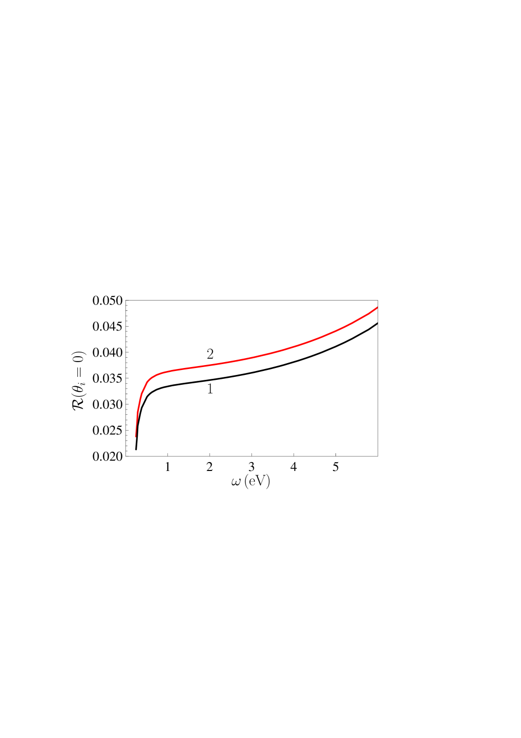
Figure 1: The reflectivities of the graphene-coated and uncoated silica plates (the lines 2 and 1, respectively) at the normal incidence are shown as functions of frequency at high frequencies.

Now we apply the developed formalism to the case of amorphous Si$\textrm{O}_{2}$ (silica) plate coated with graphene film. In all computations we use the optical data for the complex index of refraction of silica c33 tabulated in the frequency region 0.00248 eV $\leq\omega\leq$ 2000 eV. At smaller frequencies $\omega<$ 0.00248 eV it holds $n_{1}=1.956=$const, $n_{2}=0$. We start from the case of high frequencies (11). According to the results of Sec. II, this case includes the experimentally interesting regions of optical and ultraviolet frequencies. The reflectivity of the graphene-coated silica at the normal incidence as a function of frequency is computed by Eq. (16). The computational results are presented in Fig. 1 by the line 2. In the same figure line 1 shows the reflectivity of an uncoated silica plate at the normal incidence computed by Eq. (17). As can be seen in Fig. 1, in the regions of optical and ultraviolet frequencies the graphene coating slightly (from 6% to 9%) increases the reflectivity of a silica plate at the normal incidence.

Next, we consider the dependence of reflectivities on the angle of incidence at high frequencies. For this purpose, we calculate the quantities

$$\mathcal{R}^{(g,p)}_{\textrm{TM}(\textrm{TE})}(\omega,\theta_{i})=\left|R^{(g,p)}_{\textrm{TM}(\textrm{TE})}(\omega,\theta_{i})\right|^{2},$$ (23)

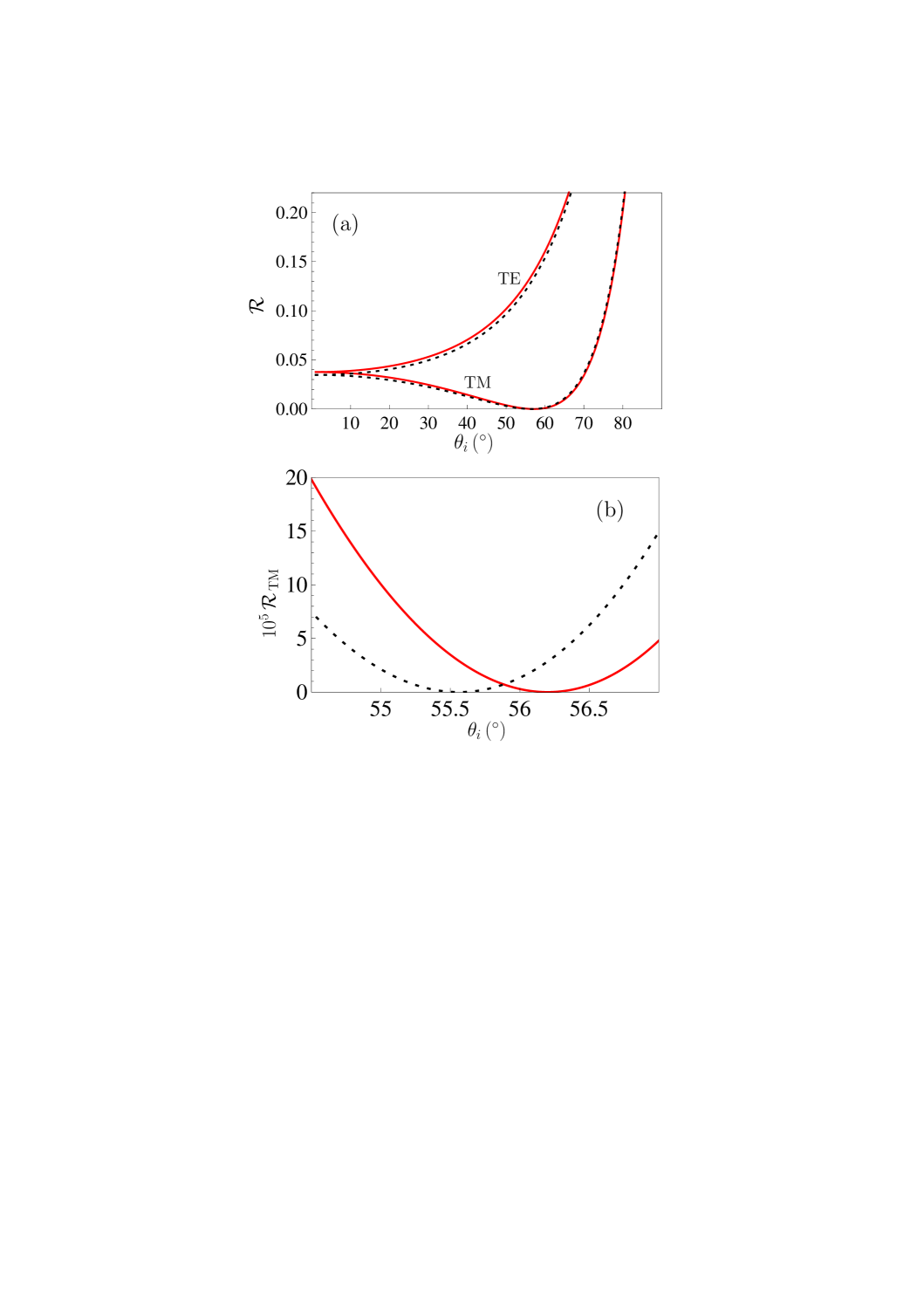
Figure 2: (a) The TM and TE reflectivities of the graphene-coated silica plate at $\omega=3\times 10^{15}$ rad/s are shown as functions of the incidence angle by the lower and upper solid lines, respectively. The dashed lines show similar results for an uncoated silica plate. (b) The TM reflectivities of graphene-coated and uncoated silica plates at $\omega=3\times 10^{15}$ rad/s are shown by the solid and dashed lines, respectively, in the vicinity of the Brewster angle.

where $R^{(g,p)}_{\textrm{TM}(\textrm{TE})}(\omega,\theta_{i})$ are given by Eqs. (2) and (13). The computational results at $\omega=2$ eV$=3\times 10^{15}$ rad/s (visible light) are presented in Fig. 2(a) as a function of $\theta_{i}$ by the lower and upper solid lines (for the TM and TE polarizations, respectively). In the same figure, the dashed lines show the computational results in the absence of graphene coating. As is seen in Fig. 2(a), the Brewster angle, at which the reflected light is fully (TE) polarized, is slightly different for the uncoated and graphene-coated silica plates. To make this effect more quantitative, in Fig. 2(b) we plot the reflectivities $\mathcal{R}_{\textrm{TM}}$ on a larger scale in the vicinity of the Brewster angle (the dashed and solid lines are for an uncoated and for a graphene-coated silica plates, respectively). As is seen in Fig. 2(b), graphene coating leads to the increase of the Brewster angle from $\theta_{\textrm{B}}=55.5^{\circ}$ to $\theta_{\textrm{B}}=56.2^{\circ}$.

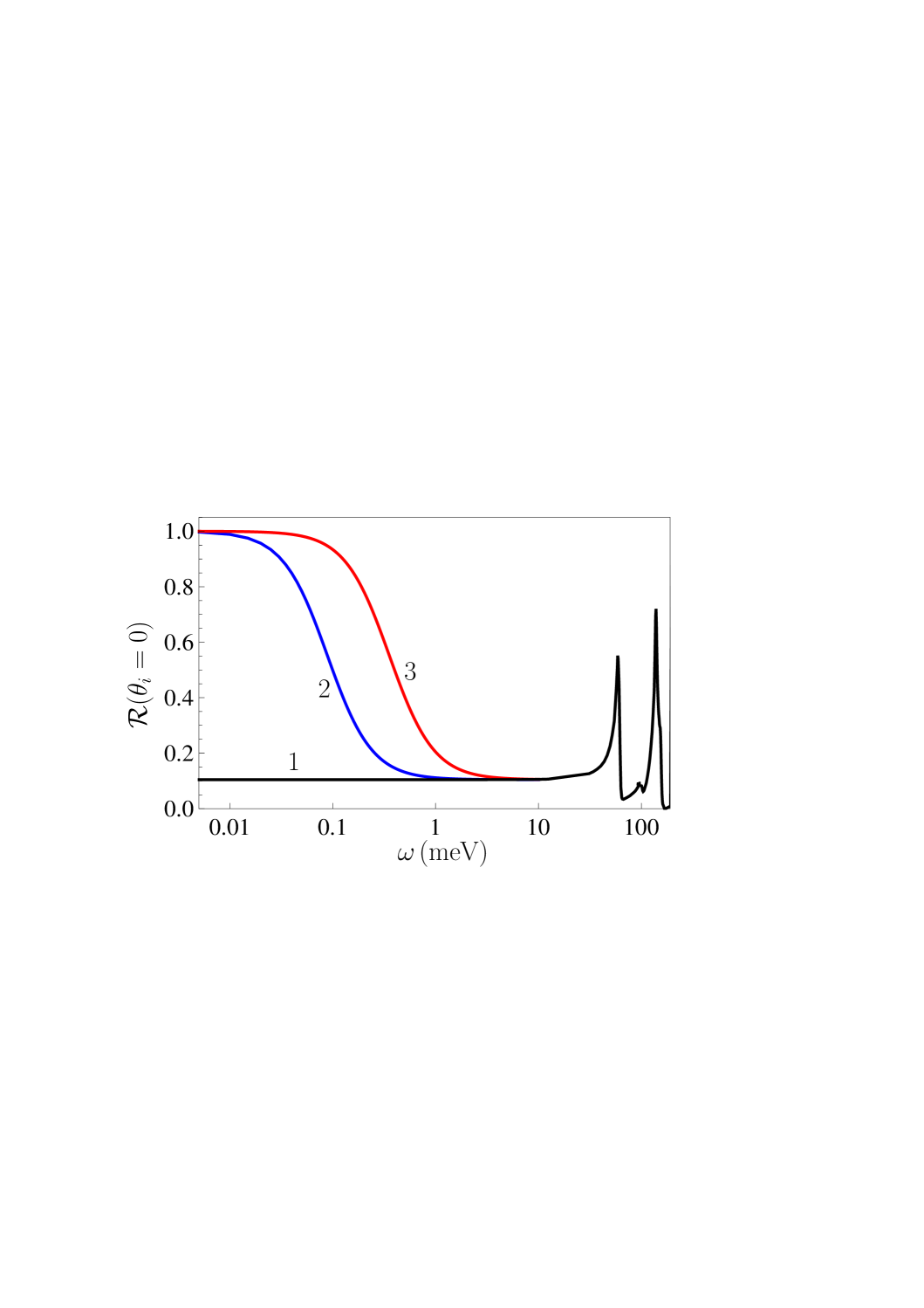
Figure 3: The reflectivities of the graphene-coated and uncoated silica plates (the lines 2, 3 and 1, respectively) at the normal incidence are shown as functions of frequency at low frequencies. The lines 2 and 3 are plotted for the graphene-coated silica at $T=75$ K and $T=300$ K, respectively.

We are coming now to the asymptotic region of low frequencies (18). In this case the reflectivity of the graphene-coated silica plate at the normal incidence is computed by Eq. (22). The computational results as a function of frequency are shown in Fig. 3 by the lines 2 and 3 at $T=75$ K and $T=300$ K, respectively. The line 1 shows the reflectivity of an uncoated silica plate at the normal incidence computed by Eq. (17). As is seen in Fig. 3, at low frequencies the graphene coating leads to significant (up to an order of magnitude) increase of the reflectivity of silica at the normal incidence. It is seen also that, unlike the case of high frequencies, there is strong dependence of the reflectivity on temperature. Thus, at $\omega=0.1,0.5$, and 1 eV the reflectivity at $T=300$ K is larger than that at $T=75$ K by the factors of 1.88, 2.91, and 1.76, respectively.

The dependence of the TM and TE reflectivities on the angle of incidence is easily obtainable by using Eqs. (2), (20) and (23). In the range of low frequencies, however, the full polarization of an incident light is not achieved at any angle.

IV Reflectivity of graphene-coated metal surfaces

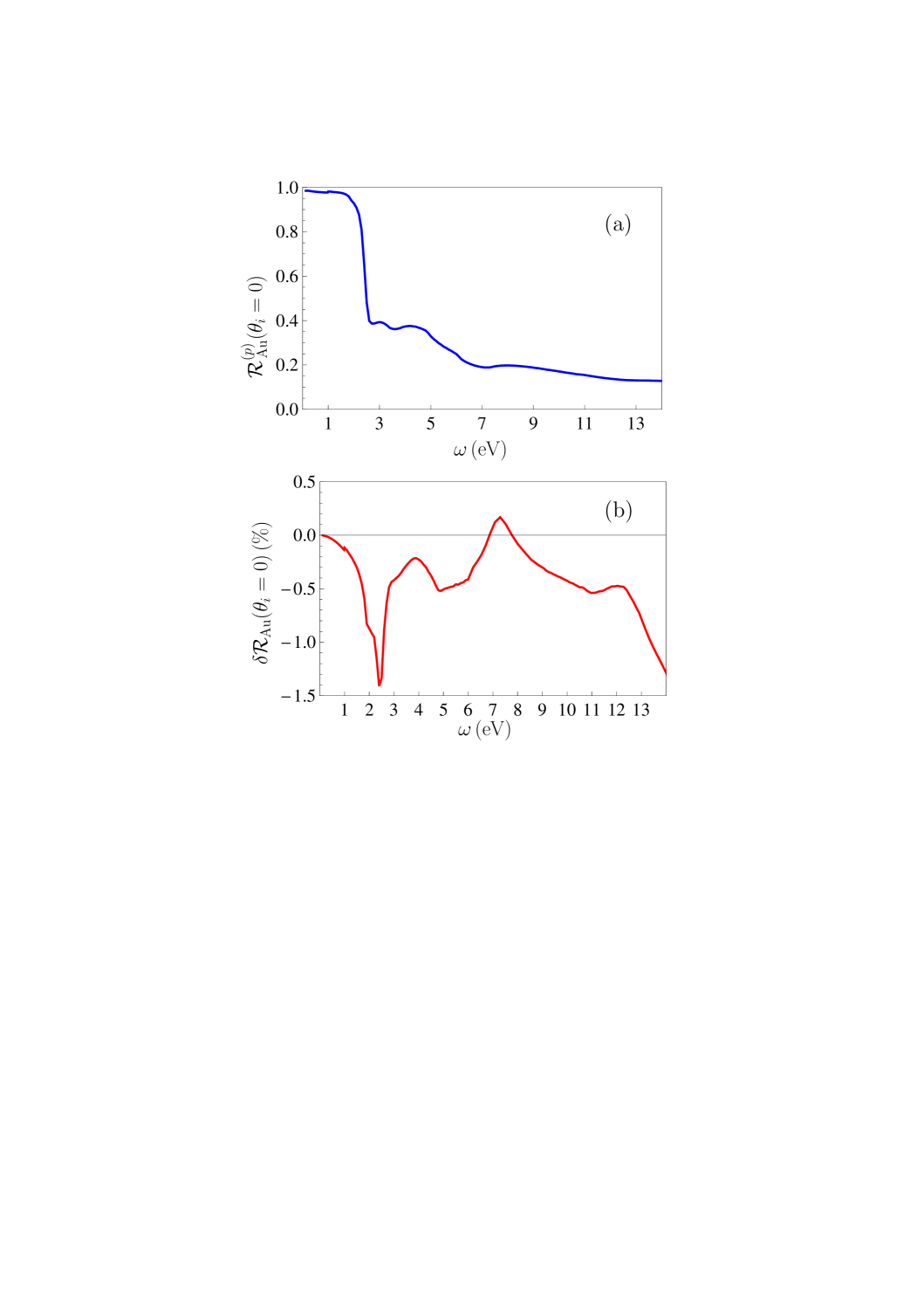
Figure 4: (a) The reflectivities of the uncoated Au plate and (b) the relative change of reflectivity of the graphene-coated Au plate at the normal incidence are shown as functions of frequency.

In this section, we consider the reflectivity properties of metal plates coated with graphene layer. We start with the case of Au plate. The complex index of refraction of Au is tabulated in Ref. c33 in the frequency region 0.125 eV $<\omega<$ 9919 eV. In the most part of this region (specifically, at $\omega>0.26$ eV) one can use the asymptotic expression at high frequencies to calculate the reflectivities of the graphene-coated Au plate. The reflectivity of an uncoated Au plate at the normal incidence is shown in Fig. 4(a) as a function of frequency. Computations were performed by using Eq. (17).

Note that the influence of graphene coating on metal surfaces is smaller than that on dielectric ones. Because of this it is not convenient to show the reflectivity of the graphene-coated Au plate in the same figure as the uncoated one. Instead, we calculate the relative quantity

$$\delta\mathcal{R}_{\textrm{Au}}(\omega,\theta_{i}=0)=\frac{\mathcal{R}^{(g,p)}_{\textrm{Au}}(\omega,0)-\mathcal{R}^{(p)}_{\textrm{Au}}(\omega,0)}{\mathcal{R}^{(p)}_{\textrm{Au}}(\omega,0)},$$ (24)

where $\mathcal{R}^{(g,p)}_{\textrm{Au}}(\omega,0)$ in the high-frequency region $\omega>0.26$ eV was computed using Eqs. (16) and (23). At lower frequencies the exact expressions (5), (6) and (8) for the polarization tensor have been used. At $\omega<0.125$ eV the optical data were extrapolated by means of the Drude model c34 . The computational results for the quantity (24) versus frequency are presented in Fig. 4(b) in the frequency range from 0.125 eV to 14 eV.

As is seen in Fig. 4(b), for an Au plate the reflectivity at the normal incidence becomes smaller due to the presence of graphene coating (this is opposite to the case of silica considered in Sec. III). The single exception from this observation is the frequency interval 6.7 eV $<\omega<$ 7.5 eV, where $\delta\mathcal{R}_{\textrm{Au}}(\omega,\theta_{i}=0)>0$. The largest in magnitude influence of graphene coating $|\delta\mathcal{R}_{\textrm{Au}}(\omega,\theta_{i}=0)|=1.4\%$ takes place at $\omega=2.4$ eV $=3.65\times 10^{15}$ rad/s. It should be stressed also that in the whole region $\omega<0.26$ eV (the moderate and low frequencies) $\delta\mathcal{R}_{\textrm{Au}}(\omega,\theta_{i}=0)=0$ with high accuracy, i.e., the graphene coating does not influence the reflectivity properties. As a result, the reflectivity of the graphene-coated Au plate does not depend on temperature. These observations are in agreement with the fact that graphene coatings do not influence the van der Waals and Casimir forces between metal plates c21 .

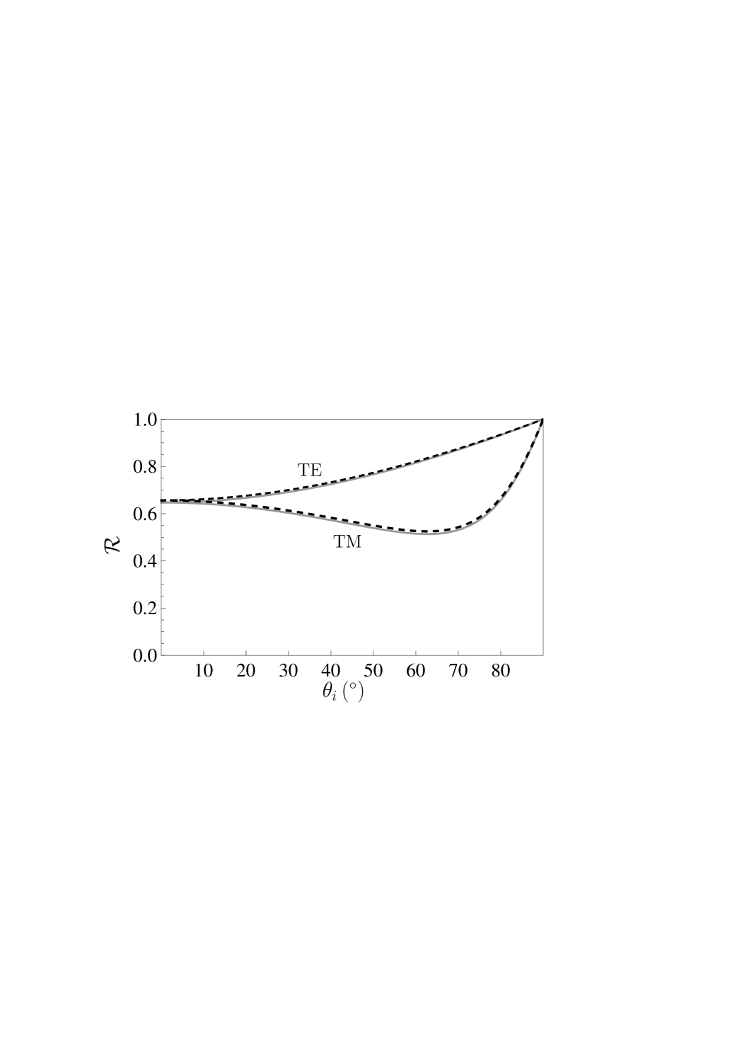
Figure 5: The TM and TE reflectivities of the graphene-coated Au plate at $\omega=3.65\times 10^{15}$ rad/s are shown as functions of the incidence angle by the lower and upper solid lines, respectively. The dashed lines show similar results for an uncoated Au plate.

It is instructive also to consider the dependences of the TM and TE reflectivities of a graphene-coated Au plate on the angle of incidence. The computational results obtained by Eqs. (2), (13) and (23) at $\omega=2.4$ eV $=3.65\times 10^{15}$ rad/s are shown in Fig. 5 (the lower and upper solid lines are for the TM and TE polarizations, respectively). The dashed lines show the computational results for an uncoated Au plate. As is seen in Fig. 5, graphene coating only slightly influences the angle dependences of the reflectivities. The full polarization of an incident light is not achieved at any frequency.

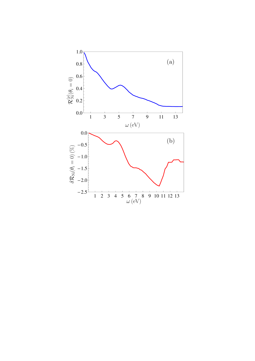
Figure 6: (a) The reflectivity of the uncoated Ni plate and (b) the relative change of reflectivity of the graphene-coated Ni plate at the normal incidence are shown as functions of frequency.

The results for the reflectivity of graphene-coated magnetic metals are somewhat different from the case of nonmagnetic ones. As an example, here we consider Ni. The optical data for the complex index of refraction of Ni in the frequency region 0.1 eV $<\omega<$ 9919 eV are also contained in Ref. c33 . The reflectivity of an uncoated Ni plate at the normal incidence is calculated by Eq. (14) and the results are presented in Fig. 6(a) in the frequency region from $0.1$ eV to $14$ eV. The comparison with Fig. 4(a) shows that at low frequencies the reflectivity of Ni decreases faster than for Au, but has no an abrupt fall in the region above 2 eV.

The relative change of reflectivity of the graphene-coated Ni is defined in the same way as that for Au in Eq. (24). It was computed as described above for Au, and the computational results versus frequency are shown in Fig. 6(b). As can be seen in this figure, for a Ni plate the reflectivity at the normal incidence becomes smaller due to presence of graphene. This is qualitatively similar to the case of Au plate. Here, however, the maximum in magnitude influence $|\delta\mathcal{R}_{\textrm{Au}}(\omega,\theta_{i}=0)|=2.5\%$ takes place not for a visible light (as it holds for Au), but at $\omega=10.4$ eV $=1.58\times 10^{16}$ rad/s, i.e., in the ultraviolet region. Similar to the case of Au, at moderate and low frequencies the graphene coating does not influence the reflectivity of Ni plate (at $\omega<0.1$ eV the optical data for Ni were extrapolated using Drude model c35 ). As a result, it does not depend on the temperature.

V Reflectivity of graphene-coated Si with different concentrations of charge carriers

Now we turn out attention to the graphene-coated Si plates, where Si may have different concentrations of charge carriers due to different dopings. We start from the case of high-resistivity dielectric Si. In this case, the optical data for the complex index of refraction are again contained in Ref. c33 over the frequency region from 0.004959 eV to 2000 eV. In the region $\omega<0.004959$ eV one has $n_{1}=3.416$, $n_{2}=0$.

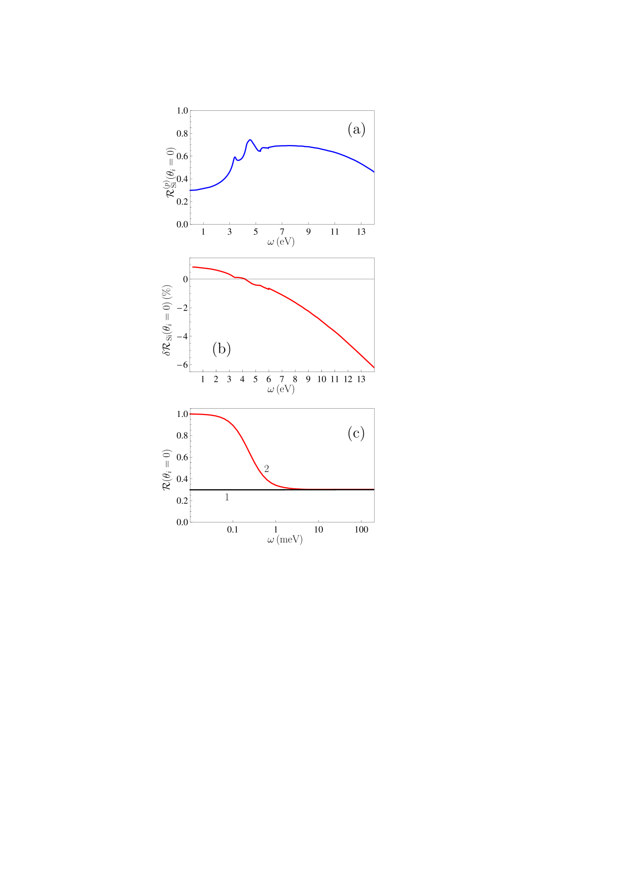
Figure 7: (a) The reflectivity of the uncoated high-resistivity Si plate, (b) the relative change of reflectivity of the high-resistivity graphene-coated Si plate, and (c) the reflectivities of the high-resistivity graphene-coated Si plate at $T=300$ K and $T=0$ K (the lines 2 and 1, respectively) at the normal incidence are shown as functions of frequency.

In Fig. 7(a) we plot the reflectivity of an uncoated dielectric Si at the normal incidence as a function of frequency computed by Eq. (17) over the entire frequency region. Computations show that in the region of high frequencies defined in Eq. (11) the impact of graphene coating achieves several percent only starting from a few eV. Because of this, for the characterization of this impact, it is convenient to use the relative change in the reflectivity of graphene-coated Si plate defined like that for Au in Eq. (24). In Fig. 7(b) the quantity $\delta\mathcal{R}_{\textrm{Si}}(\theta_{i}=0)$ is shown as a function of frequency in the region of high frequencies from 0.26 eV to 14 eV. Computations were performed by Eq. (16). As is seen in Fig. 7(b), the relative change in the reflectivity of a graphene-coated Si plate is a monotonously decreasing function of frequency. Its magnitude achieves the largest value $|\delta\mathcal{R}_{\textrm{Si}}(\omega,\theta_{i}=0)|=6\%$ at $\omega=14$ eV. It is notable that the graphene coating increases the reflectivity of a high resistivity Si plate at optical frequencies, but decreases it at ultraviolet frequencies.

We consider now the region of moderate and low frequencies $\omega<0.26$ eV = 260 meV. In this region, the asymptotic case of low frequencies (18) holds for $\omega\leq 2.6$ meV. Here, computations can be performed by Eq. (22). In the region from 2.6 meV to 0.26 eV the exact equations (2)–(8) should be used. The computational results for the reflectivity of graphene-coated high-resistivity Si plate at the normal incidence at $T=300$ K is shown in Fig. 7(c) by the line 2 as a function of frequency. In the same figure, the line 1 shows the reflectivity of an uncoated high-resistivity Si plate at the normal incidence. The line 1 to within 1% represents also the reflectivity of the graphene-coated Si plate at zero temperature. As is seen in Fig. 7(c), the role of graphene coating increases with decreasing frequency. At $\omega=0.01$ meV the reflectivity of the graphene-coated Si is larger than for the uncoated one by the factor of 3.33. Another conclusion is that for high-resistivity Si the total role of graphene coating is provided by the thermal effect. At $\omega>4$ meV both the relative impact of graphene coating on the reflectivity at the normal incidence and, correspondingly, the thermal effect are in the limits of 1%. The impact of the graphene coating again becomes larger in magnitude only in the region of high frequencies [see Fig. 7(b)], where it does not depend on the temperature.

Next, we consider the case of doped low-resistivity Si plates with some concentrations of charge carriers. In this case the dielectric permittivity of the plate material can be presented in the form

$$\epsilon(\omega)=[n_{1}(\omega)+in_{2}(\omega)]^{2}=\epsilon_{d}(\omega)-\frac{\omega_{p}^{2}}{\omega(\omega+i\gamma)},$$ (25)

where $\epsilon_{d}(\omega)=[n_{1d}(\omega)+in_{2d}(\omega)]^{2}$ is the dielectric permittivity of high-resistivity Si and $n_{1d}(\omega)$, $n_{2d}(\omega)$ are the used above tabulated optical data for its complex index of refraction c33 . The free charge carriers are taken into account by means of the Drude-like term, where $\omega_{p}$ is the plasma frequency and $\gamma$ is the relaxation parameter. As a result, the real and imaginary parts $n_{1}(\omega)$ and $n_{2}(\omega)$ of the complex refraction index of the low-resistivity Si are calculated from the following system of equations:

$$\begin{split}&n_{1}^{2}(\omega)-n_{2}^{2}(\omega)=n_{1d}^{2}(\omega)-n_{2d}^{2}(\omega)-\frac{\omega_{p}^{2}}{\omega^{2}+\gamma^{2}},\\ &n_{1}(\omega)n_{2}(\omega)=n_{1d}(\omega)n_{2d}(\omega)+\frac{\omega_{p}^{2}\gamma}{2\omega(\omega^{2}+\gamma^{2})}.\end{split}$$ (26)

Calculations using Eq. (26) show that in the asymptotic region of high frequencies the presence of free charge carriers leads to only a negligibly small change of the complex index of refraction, as compared to the case of dielectric Si. Because of this, in the region of high frequencies the influence of graphene coating on the reflectivity of low-resistivity Si plate is again shown by Fig. 7(b).

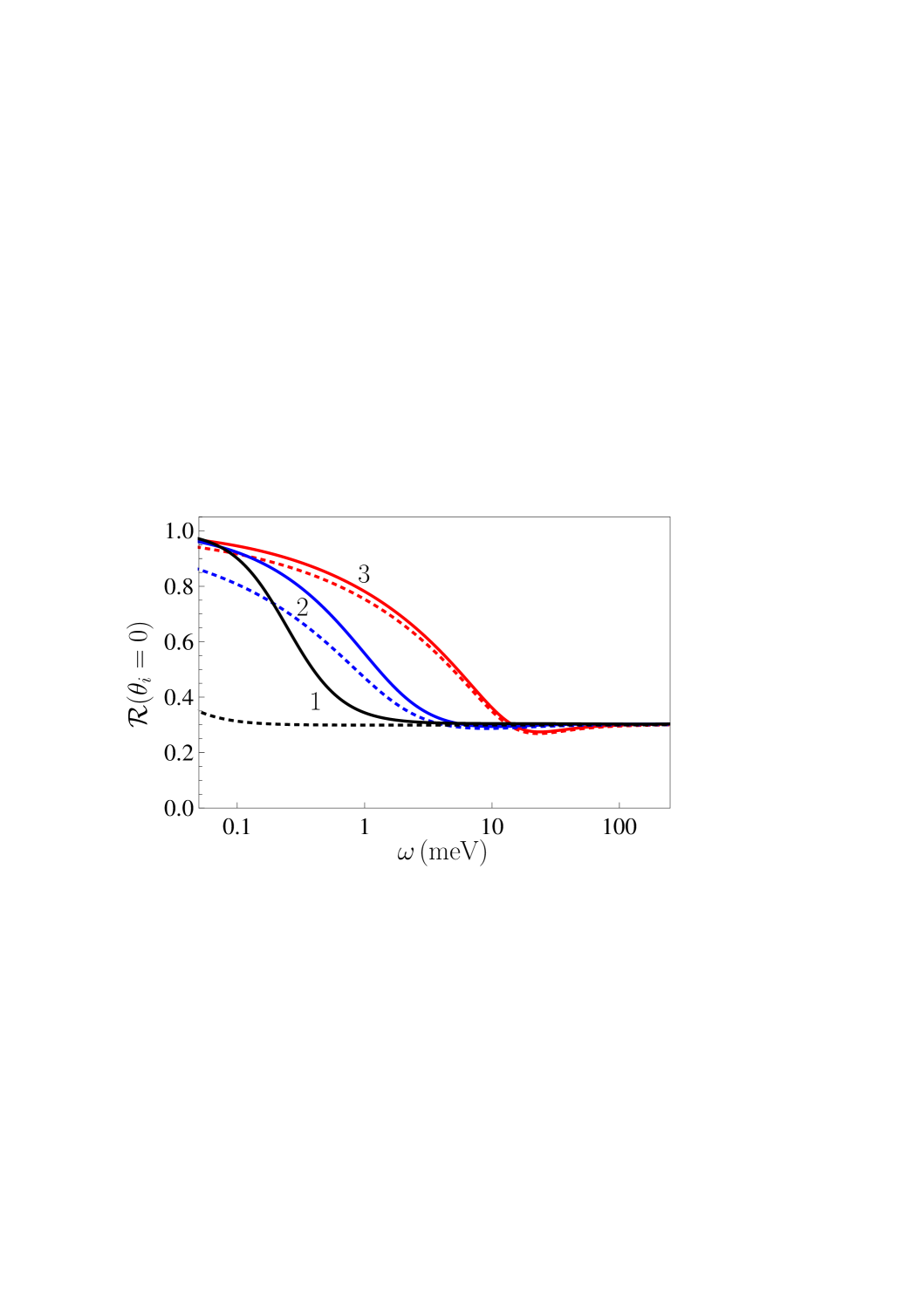
Figure 8: The reflectivities of the low-resistivity graphene-coated Si plates are shown at $T=300$ K by the solid lines 1, 2, and 3 as functions of frequency for the concentrations of free charge carriers equal to $5\times 10^{14}$, $5\times 10^{16}$, and $5\times 10^{17}\text{cm}^{-3}$, respectively. The respective quantities for the uncoated plates are shown by the dashed lines 1, 2, and 3.

Now we perform computations of the reflectivity of low-resistivity P-doped Si at the normal incidence in the region of moderate and low frequencies $\omega<0.26$ eV. As above, for $\omega\leq 2.6$ meV the asymptotic equation (18) was used. In the frequency interval 2.6 meV$<$0.26 eV computations were performed by the exact equations (2)–(8). The computational results at $T=300$ K as a function of frequency are shown in Fig. 8 by the solid lines 1, 2, and 3 for the concentrations of charge carriers $N_{1}=5\times 10^{14}\text{cm}^{-3}$, $N_{2}=5\times 10^{16}\text{cm}^{-3}$, and $N_{3}=5\times 10^{17}\text{cm}^{-3}$. At these concentrations, the respective resistivities $\rho_{i}$ were obtained from Ref. c36 and the Drude parameters were found from the equations c37

$$\omega_{p,i}=\frac{e\sqrt{4\pi N_{i}}}{\sqrt{m^{*}}},\qquad\gamma_{i}=\frac{\rho_{i}\omega_{p,i}^{2}}{4\pi},$$ (27)

where $m^{*}=0.26m_{e}$ is the effective mass, $m_{e}$ is the electron mass, with the results $\omega_{p,1}=2.5\times 10^{12}$ rad/s, $\omega_{p,2}=2.5\times 10^{13}$ rad/s, $\omega_{p,3}=7.8\times 10^{13}$ rad/s; $\gamma_{1}=1.1\times 10^{13}$ rad/s, $\gamma_{2}=2.2\times 10^{13}$ rad/s, and $\gamma_{3}=3.8\times 10^{13}$ rad/s. The dashed lines 1, 2, and 3 show the reflectivities at the normal incidence of the respective uncoated low-resistivity Si plates. As is seen in Fig. 8, the impact of graphene coating on the reflectivity quickly decreases with increasing concentration of charge carriers and increasing frequency.

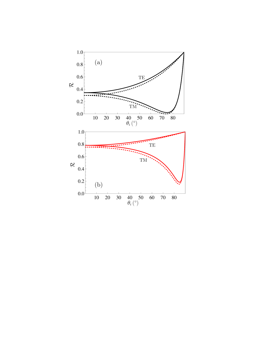
Figure 9: The TM and TE reflectivities of the graphene-coated low-resistivity Si plate at $\omega=1.5\times 10^{12}$ rad/s are shown at $T=300$ K as functions of the incidence angle by the lower and upper solid lines, respectively, for the doping concentrations (a) $N=5\times 10^{14}\text{cm}^{-3}$ and (b) $N=5\times 10^{17}\text{cm}^{-3}$. The dashed lines show similar results for an uncoated Si.

The dependences of the TM and TE reflectivities of the graphene-coated plate made of low-resistivity Si on the angle of incidence at low frequencies can be calculated by Eqs. (2), (20), and (23). The computational results at $\omega=1$ meV$=1.5\times 10^{12}$ rad/s, $T=300$K are shown in Fig. 9 by the lower and upper solid lines for the TM and TE polarizations, respectively (the dashed lines demonstrate the respective results for an uncoated low-resistivity Si plate). In Figs. 9(a) and 9(b) the concentrations of charge carriers were chosen to be $N=5\times 10^{14}$ and $5\times 10^{17}\text{cm}^{-3}$, respectively. As is seen in Fig. 9(a), for a lower conductivity uncoated Si plate the Brewster angle is equal to $\theta_{i}\approx 73.5^{\circ}$. For the graphene-coated plate, however, the full polarization of the reflected light does not happen at any incidence angle (the minimum value $\mathcal{R}_{\mathrm{TM}}\approx 0.022$ is achieved at $\theta_{i}\approx 74.3^{\circ}$). For a higher conductivity Si [Fig. 9(b)] the full polarization does not happen either for an uncoated or for a graphene-coated plate. The minimum values $\mathcal{R}_{\mathrm{TM}}\approx 0.15$ and 0.18 are achieved at $\theta_{i}=84^{\circ}$ and $84.8^{\circ}$ for an uncoated and graphene-coated plates, respectively.

At the end of this section, we note that for Si plates with the highest doping concentrations ($\sim 10^{20}\;\text{cm}^{-3}$) there is no influence of graphene coating on the reflectivity properties. In the region of high frequencies this fact was already discussed above, and at low frequencies the situation is the same as for metals considered in Sec. IV.

VI Conclusions and Discussion

In the foregoing, we have developed theoretical description for the reflectivity properties of the graphene-coated plates made of different materials (dielectric, metal and semiconductor). This theory is based on the Dirac model of graphene, which is described by the recently found polarization tensor in (2+1)-dimensional space-time, allowing the analytic continuation to the real frequency axis c27 . The materials of the plate are described by the frequency-dependent complex index of refraction. In the framework of this theory, the general formulas are obtained for the reflection coefficients and reflectivities of graphene-coated plates, and their analytic asymptotic expressions at both high and low frequencies.

The developed theory is applied to the cases of graphene-coated dielectric, metal, and semiconductor plates. It is shown that for a dielectric material (fused silica) in the region of optical and ultraviolet frequencies the reflectivity of the graphene-coated plate at the normal incidence is by several percent larger than of an uncoated one. In this frequency region, the graphene coating also results in some increase of the Brewster angle. In the asymptotic region of low frequencies, graphene coating is shown to significantly (up to an order of magnitude) increase the reflectivity of silica at the normal incidence. This effect is completely determined by the thermal corrections at room temperature.

For metals, the developed theory is illustrated by the examples of Au and Ni plates. In the case of high and moderate frequencies, we have shown that the graphene coating decreases the plate reflectivity at the normal incidence. For low frequencies the graphene coating does not influence the reflectivities of Au and Ni plates.

We have also applied the developed theory to graphene-coated semiconductor plates (Si with various concentrations of charge carriers). For the high-resistivity Si plate, the influence of graphene coating at high frequencies achieves several percent similar to the case of a silica plate. In the region of moderate and low frequencies, the graphene coating can significantly increase the reflectivity of Si plate at the normal incidence. For the low-resistivity Si the effect of graphene coating was investigated at different concentrations of charge carriers. It is shown that at high frequencies the graphene coating does not influence the reflecting properties. In the region of low frequencies the impact of graphene coating on the reflectivity of Si plate at the normal incidence quickly decreases with increasing concentration of charge carriers and increasing frequency. The dependences of the reflectivities on the angle of incidence were also computed. According to our results, the graphene coating increases the reflectivities of low-resistivity Si at low frequencies. The full polarization of the reflected light is not achieved at any angle of incidence.

As was noted in Sec. I, the theory of reflectivity properties of graphene-coated material plates is of interest in many technological applications using graphene coatings, such as the optical detectors, transparent conductors, anti-reflection surfaces in solar-cells etc. In the future, it is planed to generalize the developed formalism to the case of graphene with nonzero mass-gap parameter and chemical potential. It would be useful also to apply it to thin material plates (films) coated with graphene.

References

- (1) M. I. Katsnelson, Graphene: Carbon in two Dimensions (Cambridge University Press, Cambridge, 2012).
- (2) A. H. Castro Neto, F. Guinea, N. M. R. Peres, K. S. Novoselov, and A. K. Geim, Rev. Mod. Phys. 81, 109 (2009).
- (3) M. O. Goerbig, Rev. Mod. Phys. 83, 1193 (2011).
- (4) M. I. Katsnelson, K. S. Novoselov, and. A. K. Geim, Nat. Phys. 2, 620 (2006).
- (5) D. Allor, T. D. Cohen, and D. A. McGady, Phys. Rev. D 78, 096009 (2008).
- (6) C. G. Beneventano, P. Giacconi, E. M. Santangelo, and R. Soldati, J. Phys A: Math. Theor. 42, 275401 (2009).
- (7) G. L. Klimchitskaya and V. M. Mostepanenko, Phys. Rev. D 87, 215011 (2013).
- (8) G. Gómez-Santos, Phys. Rev. B 80, 245424 (2009).
- (9) D. Drosdoff and L. M. Woods, Phys. Rev. B 82, 155459 (2010).
- (10) D. Drosdoff and L. M. Woods, Phys. Rev. A 84, 062501 (2011).
- (11) Bo E. Sernelius, Europhys. Lett. 95, 57003 (2011).
- (12) Bo E. Sernelius, Phys. Rev. B 85, 195427 (2012).
- (13) A. D. Phan, L. M. Woods, D. Drosdoff, I. V. Bondarev, and N. A. Viet, Appl. Phys. Lett. 101, 113118 (2012).
- (14) M. Bordag, G. L. Klimchitskaya, U. Mohideen, and V. M. Mostepanenko, Advances in the Casimir Effect (Oxford University Press, Oxford, 2015).
- (15) M. Bordag, I. V. Fialkovsky, D. M. Gitman, and D. V. Vassilevich, Phys. Rev. D 80, 245406 (2009).
- (16) I. V. Fialkovsky, V. N. Marachevsky, and D. V. Vassilevich, Phys. Rev. B 84, 035446 (2011).
- (17) M. Bordag, G. L. Klimchitskaya, and V. M. Mostepanenko, Phys. Rev. B 86, 165429 (2012).
- (18) M. Chaichian, G. L. Klimchitskaya, V. M. Mostepanenko, and A. Tureanu, Phys. Rev. A 86, 012515 (2012).
- (19) G. L. Klimchitskaya and V. M. Mostepanenko, Phys. Rev. B 87, 075439 (2013).
- (20) G. L. Klimchitskaya, V. M. Mostepanenko, and Bo E. Sernelius, Phys. Rev. B 89, 125407 (2014).
- (21) G. L. Klimchitskaya, U. Mohideen, and V. M. Mostepanenko, Phys. Rev B 89, 115419 (2014).
- (22) G. L. Klimchitskaya and V. M. Mostepanenko, Phys. Rev A 89, 052512 (2014).
- (23) A. A. Banishev, H. Wen, J. Xu, R. K. Kawakami, G. L. Klimchitskaya, V. M. Mostepanenko, and U. Mohideen, Phys. Rev. B 87, 205433 (2013).
- (24) G. L. Klimchitskaya and V. M. Mostepanenko, Phys. Rev. B 91, 045412 (2015).
- (25) L. A. Falkovsky and S. S. Pershoguba, Phys. Rev. B 76, 153410 (2007).
- (26) T. Stauber, N. M. R. Peres, and A. K. Geim, Phys. Rev. B 78, 085432 (2008).
- (27) G. L. Klimchitskaya, V. M. Mostepanenko, and V. M. Petrov, in Internet of Things, Smart Spaces, and Next Generation Networks and Systems, edited by S. Balandin, S. Andreev, and Y. Koucheryavy (Springer, New York, 2014), p 451.
- (28) M. Bordag, G. L. Klimchitskaya, V. M. Mostepanenko, and V. M. Petrov, Phys. Rev. D 91, 045037 (2015).
- (29) G. L. Klimchitskaya and V. M. Mostepanenko, Phys. Rev B 91, 174501 (2015).
- (30) X. Jiang, Y. Cao, K. Wang, J. Wei, D. Wu, H. Zhu, Surf, Coatings Technology 261, 327 (2015).
- (31) S. Watcharotone, D. A. Dikin, S. Stankovich et al., Nano Lett. 7, 1888 (2007).
- (32) Springer Handbook of Nanomaterials, edited by R. Vajtai (Springer, Berlin, 2013).
- (33) L. F. Dumée, L. He, Z. Wang et al., Carbon 87, 395 (2015).
- (34) Handbook of Optical Constants of Solids, edited by E.D. Palik (Academic, New York, 1985).
- (35) C.-C. Chang, A. A. Banishev, R. Castillo-Garza, G. L. Klimchitskaya, V. M. Mostepanenko and U. Mohideen, Phys. Rev. B 85, 165443 (2012).
- (36) A. A. Banishev, G. L. Klimchitslaya, V. M. Mostepanenko, and U. Mohideen, Phys. Rev. B 88, 155410 (2013).
- (37) http://www.ioffe.rssi.ru/SVA/NSM/Semicond/Si/electric.html.
- (38) N. W. Ashcroft and N. D. Mermin, Solid State Physics (Saunders College, Philadelphia, 1976).