Edge-enhancing Filters with Negative Weights

Abstract

In [doi:10.1109/ICMEW.2014.6890711], a graph-based denoising is performed by projecting the noisy image to a lower dimensional Krylov subspace of the graph Laplacian, constructed using nonnegative weights determined by distances between image data corresponding to image pixels. We extend the construction of the graph Laplacian to the case, where some graph weights can be negative. Removing the positivity constraint provides a more accurate inference of a graph model behind the data, and thus can improve quality of filters for graph-based signal processing, e.g., denoising, compared to the standard construction, without affecting the costs.

I Introduction

Constructing efficient signal filters is a fundamental problem in signal processing with a vast literature; see, e.g., recent papers [1, 2, 3, 4, 5, 6] and references there. A filter can be described by a transformation $F$, often non-linear, of an input signal, represented by a vector $x$, into a filtered signal, represented by a vector $F(x)$. We revisit some classical constructions of filters aimed at signal noise reduction, with the emphasis on bilateral filter, popular in image denoising [7, 8, 9, 10]. The goal of the filter is signal smoothing, reducing a high oscillatory additive noise. The smoothing can be achieved by averaging, which can be typically interpreted as a low-pass filter, minimizing the contribution in the filtered signal of highly oscillatory modes, treated as eigevectors of a graph Laplacian; see, e.g., [11].

It is desirable to preserve edges in the ideal noise-free signal, even at the costs of an increased PSNR. Edge-conscious filters detect, often implicitly, the locations of the edges and attempt using less aggressive or anisotropic averaging at these locations. Fully automatic edge detection in a noisy signal is difficult, typically resulting in non-linear filters, i.e. where the filtered vector $F(x)$ depends non-linearly on the input vector $x.$ However, it can be assisted by a guiding signal, having the edges in the same locations as in the ideal signal; see, e.g., [3, 12, 13].

Graph signal processing, introducing eigenvectors of the graph Laplacian as natural extensions of the Fourier bases, sheds new light at image processing; see, e.g., [14, 15, 16, 17]. In [18], graph-based filtering of noisy images is performed by directly computing a projection of the image to be filtered onto a lower dimensional Krylov subspace of the normalized graph Laplacian, constructed using nonnegative graph weights determined by distances between image data corresponding to image pixels. We extend the construction of the graph Laplacian to the case, where some weights can be negative, radically departing from the traditional assumption.

II Preliminaries

Let us for simplicity first assume that the guiding signal, denoted by $y$, is available and can be used to reliably detect the locations of the edges and, most importantly, to determine the edge-conscious linear transformation (matrix) $F_{y}$ such that the action of the filter $F(x)$ is given by the following matrix-vector product $F_{y}x=F(x).$ Having a specific construction of the guided filter matrix $F_{y}$ as a function of $y$, one can define a self-guided non-linear filter, e.g., as $F_{x}x$, which can be applied iteratively, starting with the input signal vector $x_{0}$ as follows, $x_{i+1}=F(x_{i}),\,i=0,1,\ldots,m$; cf., e.g., [19].

Similarly, an iterative application of the linear guided filter can be used, mathematically equivalent to applying the powers of the square matrix $F_{y}$, i.e. $x_{m}=\left(F_{y}\right)^{m}x_{0}$, thus naturally called the power method, which is an iterative form of PCA; see, e.g.,[20, 21]. To avoid a re-normalization of the filtered signal, it is convenient to construct the matrix $F_{y}$ in the form $F_{y}=D_{y}^{-1}W_{y}$, where entries of the square matrix $W_{y}$ are called weighs. The matrix $D_{y}$ is diagonal, made of row-sums of the matrix $W_{y}$, which are assumed to be non-zero. Thus, $D_{y}^{-1}W_{y}$ multiplied by a column-vector of ones, gives again the column-vector of ones.

Let us further assume that the matrix $W_{y}$ is symmetric and that all the entries (weighs) in $W_{y}$ are nonnegative. For signal denoising, the following observations are the most important. The right eigenvector $v_{1}$ of the matrix $D_{y}^{-1}W_{y}$ with the eigenvalue $\mu_{1}=1$ is trivial, just made of ones, only affecting the signal offset. Since the iterative matrix $F_{y}=D_{y}^{-1}W_{y}$ is diagonalizable, the power method gives

$$x_{m}=\left(F_{y}\right)^{m}x_{0}=\Sigma_{j}\;\mu_{j}^{m}\left(v_{j}^{T}Dx_{0}\right)v_{j},$$ (1)

where $1=|\mu_{1}|\geq|\mu_{2}|\geq\ldots$ are the eigenvalues of the matrix $D_{y}^{-1}W_{y}$ corresponding to the eigenvectors $v_{j}$ scaled such that $v_{i}^{T}Dv_{j}=\delta_{ij}$. The power method, according to (1), suppresses contributions of the eigenvectors corresponding to the smallest eigenvalues. Thus, the matrix $W_{y}$ needs to be constructed in such a way that these eigenvectors represent the noisy part of the input signal, while the other eigenvectors are edge-conscious; cf. anisotropic diffusion [22, 23, 24].

Let us introduce the guiding Laplacian $L_{y}=D_{y}-W_{y}$ and normalized Laplacian $D_{y}^{-1}L_{y}=I-D_{y}^{-1}W_{y}$ matrices. In [18], the power method (1) is replaced with a projection of the image vector $x$ to be denoised onto a lower dimensional Krylov subspace of the guiding normalized graph Laplacian $D_{y}^{-1}L_{y}$ and implemented, e.g., using the Conjugate Gradient (CG) method; see, e.g., [25, 26, 27].

III Motivation

One of the most popular edge-preserving denoising filters is the bilateral filter (BF), see, e.g., [28, 29] and references there, which takes the weighted average of the nearby pixels. The weights $w_{ij}$ may depend on spatial distances and signal data similarity, e.g.,

$$w_{ij}=\exp\left(-\frac{\left\|p_{i}-p_{j}\right\|^{2}}{2\sigma_{d}^{2}}\right)\exp\left(-\frac{\left\|y[i]-y[j]\right\|^{2}}{2\sigma_{r}^{2}}\right),$$ (2)

where $p_{i}$ denotes the position of the pixel $i$, the value $y[i]$ is the signal intensity, and $\sigma_{d}$ and $\sigma_{r}$ are filter parameters. To simplify the presentation and our arguments, we further assume that the signal is scalar on a one-dimensional uniform grid, setting without loss of generality the first multiplier in (2) to be $1$, and that the weights $w_{ij}$ are computed only for the nearest neighbors and set to zero otherwise.

Let us start with a constant signal, where $y[i]-y[j]=0$. Then, $w_{i-1\,i}=w_{i\,i}=w_{i\,i+1}=1$ and the graph Laplacian $L_{y}=D_{y}-W_{y}$ is a tridiagonal matrix that has nonzero entries $1$ and $-1$ in the first row, $-1$ and $1$ in the last row, and $[-1\,\;2\,-1]$ in every other row. This is a standard three-point-stencil finite-difference approximation of the negative second derivative of functions with homogeneous Neumann boundary conditions, i.e., vanishing first derivatives at the end points of the interval. Its eigenvectors are the basis vectors of the discrete cosine transform; see the first five low frequency eigenmodes (the eigenvectors corresponding to the smallest eigenvalues) of $L_{y}$ in Figure 1.

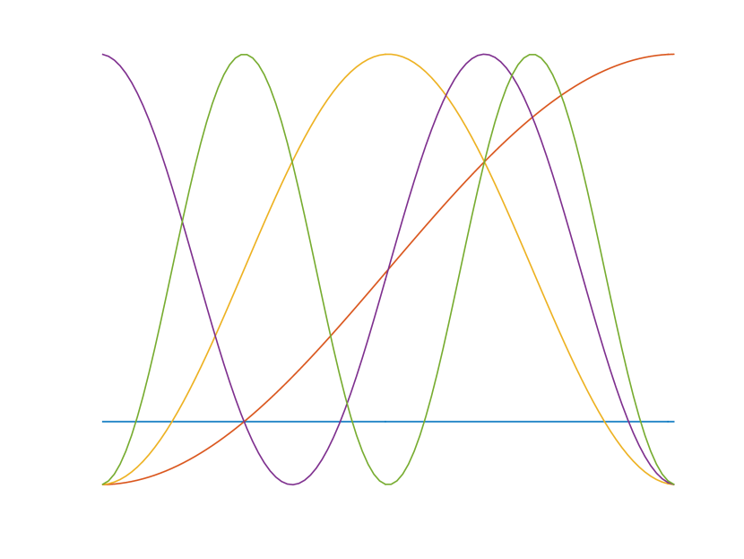
Figure 1: Discrete cosine transform low frequency modes.

As can be seen in Figure 1, all smooth low frequency eigenmodes turn flat at the end points of the interval, due to the Neumann conditions.

The key observation is that the Laplacian row sums in the first and last rows vanish for any signal, according to the standard construction of the graph Laplacian, no matter what formulas for the weights are being used! Thus, any low pass filter based on low frequency eigenmodes of the graph Laplacian flattens the signal at the end points.

Let us now use formula (2) for a piece-wise constant guiding signal $y$ with the jump large enough to result in a small value $w_{i\,i+1}=w_{i+1\,i}$ for some index $i$. The first five vectors of the corresponding Laplacian are shown in Figure 2.

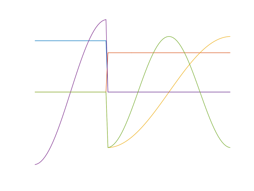
Figure 2: Edge-preserving low frequency eigenmodes.

All the plotted in Figure 2 vectors are aware of the jump, representing an edge in our one-dimensional signal $y$, but they are also all flat on both sides of the edge! Such a flatness is expected to appear for any guiding signal $y$ giving a small value $w_{i\,i+1}=w_{i+1\,i}$.

The presence of the flatness in the low frequency modes of the graph Laplacian $L_{y}$ on both sides of the edge in the guiding signal $y$ is easy to explain. When the value $w_{i\,i+1}=w_{i+1\,i}$ is small relative to other entries, the matrix $L_{y}$ becomes nearly block diagonal, with two blocks, which approximate graph Laplacian matrices of the signal $y$ restricted to sub-intervals of the signal domain to the left and to the right of the edge.

The low frequency eigenmodes of the graph Laplacian $L_{y}$ approximate combinations of the low frequency eigenmodes of the graph Laplacians on the sub-intervals. But each of the low frequency eigenmodes of the graph Laplacian on the sub-interval suffers from the flattening effect on both ends of the sub-interval, as explained above. Combined, it results in the flatness in the low frequency modes of the graph Laplacian $L_{y}$ on both sides of the edge. For denoising, the flatness of the vectors determining the low-pass filter may have a negative effect for self-guided denoising even of piece-wise constant signals, if the noise is large enough relative to the jump in the signal, as shown in Section V.

The attentive reader notices that method (1) is based on $D_{y}^{-1}W_{y}$, related to the normalized graph Laplacian $D_{y}^{-1}L_{y}$, not the Laplacian $L_{y}$ used in our arguments above. Although the diagonal matrix $D_{y}$ is not a scalar identity, and so the eigenvectors of $D_{y}^{-1}L_{y}$, not plotted here, and of $L_{y}$ are different, the difference is not qualitative enough to noticeably change the figures and invalidate our explanation.

IV Negative weights in spectral graph partitioning and for signal edge enhancing

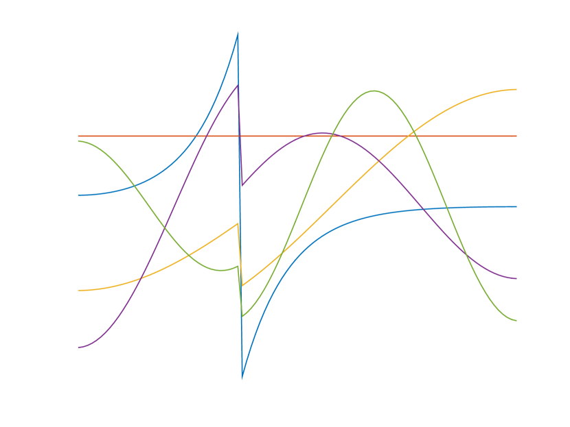
Figure 3: Edge-enhancing low frequency eigenmodes, small negative.

The low frequency eigenmodes of the graph Laplacian play a fundamental role in spectral graph partitioning, which is one of the most popular tools for data clustering; see, e.g., [30, 31, 32]. A limitation of the conventional spectral clustering approach is embedded in its definition based on the weights of graph, which must be nonnegative, e.g., based on a distance measuring relative similarities of each pair of points in the dataset. For the dataset representing values of a signal, e.g., pixel values of an image, formula (2) is a typical example of determining the nonnegative weights, leading to the graph adjacency matrix $W_{y}$ with nonnegative entries, as assumed in Section II and in all existing literature.

In applications, data points may represent feature vectors or functions, allowing the use of correlation for their pairwise comparison. The correlation can be negative, or, more generally, points in the dataset can be dissimilar, contrasting each other. In conventional spectral clustering, the only available possibility to handle such a case is to replace the anticorrelation, i.e. negative correlation, of the data points with the uncorrelation, i.e. zero correlation. The replacement changes the corresponding negative entry in the graph adjacency matrix to zero, to enable the conventional spectral clustering to proceed, but nullifies a valid comparison.

A common motivation of spectral clustering comes from analyzing a mechanical vibration model in a spring-mass system, where the masses that are tightly connected have a tendency to move synchronically in low-frequency free vibrations; e.g., [33]. Analyzing the signs of the components corresponding to different masses of the low-frequency vibration modes of the system allows one to determine the clusters. The mechanical vibration model may describe conventional clustering when all the springs are pre-tensed to create an attracting force between the masses. However, one can pre-tense some of the springs to create repulsive forces!

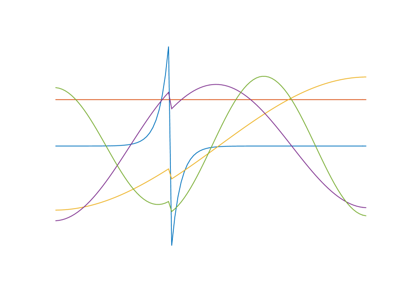
Figure 4: Edge-enhancing low frequency eigenmodes, more negative.

In the context of data clustering formulated as graph partitioning, that corresponds to negative entries in the adjacency matrix. The negative entries in the adjacency matrix are not allowed in conventional graph spectral clustering. Nevertheless, the model of mechanical vibrations of the spring-mass system with repulsive springs remains valid, motivating us to consider the effects of negative graph weights.

In the spring-mass system, the masses, which are attracted, would move together synchronically in the same direction in low-frequency free vibrations, while the masses, which are repulsed, have the tendency to move synchronically in the opposite direction. Using negative, rather than zero, weights at the edge of the guiding signal $y$ for the purposes of the low-pass filters thus is expected to repulse the flatness of low frequency eigenmodes of the graph Laplacian $L_{y}$ on the opposite sides of the edge of the signal $y$, making the low frequency eigenmodes to be edge-enhancing, rather than just edge-preserving; cf. [34] on sharpening.

Figures 3 and 4 demonstrate the effect of edge-enhancing, as a proof of concept. Both Figures 3 and 4 display the five eigenvectors for the five smallest eigenvalues of the same tridiagonal graph Laplacian as that corresponding to Figure 2 except that the small positive entry of the weights $w_{i\,i+1}=w_{i+1\,i}$ for the same $i$ is substituted by $-0.05$ in Figure 3 and by $-0.2$ in Figure 4. The previously flat around the edge eigenmodes in Figure 2 are repelled in opposite directions on the opposite sides of the edge in Figures 3 and 4.

Negative weights require caution, since even small changes dramatically alter the behaviors of the low frequency eigenmodes around the edge, as seen in Figures 3 and 4. Making the negative value more negative, we observe by comparing Figure 3 to Figure 4 that the leading eigenmode, displayed using the blue color in both figures, corresponding to the smallest nonzero eigenvalue forms a narrowing layer around the signal edge, while other eigenmodes become less affected by the change in the negative value.

V Edge-enhancing filters

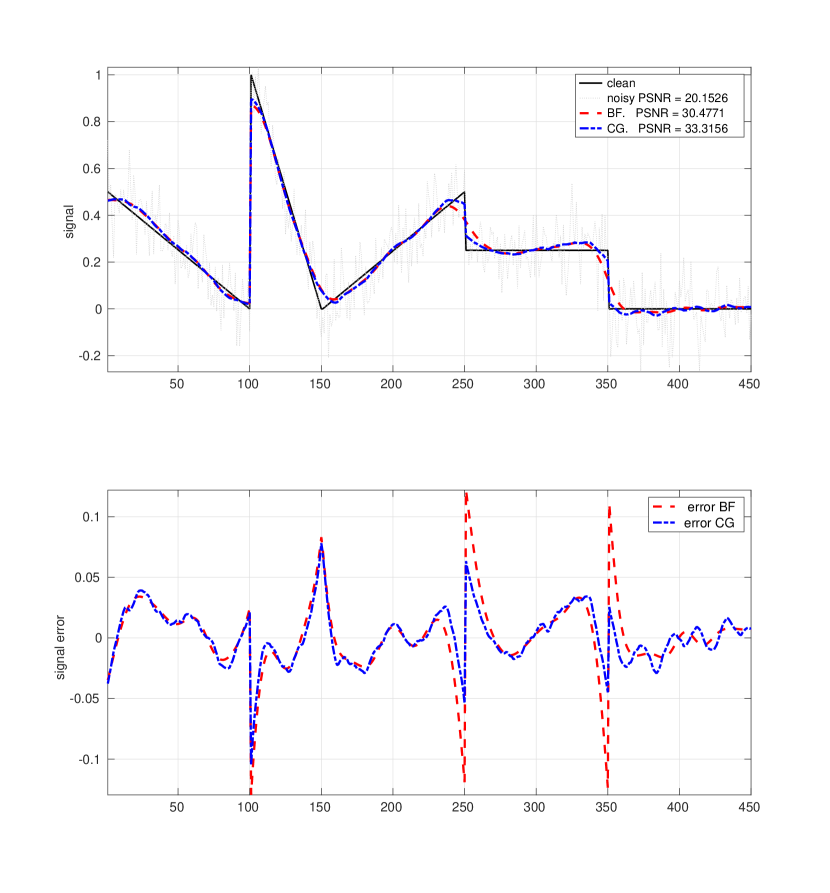
Figure 5: Edge-preserving filtering.

In this section, as a proof of concept, we numerically test the proposed edge-enhancing filters on a toy one-dimensional example using the classical nonlinear self-guiding BF and a guided (by a noiseless signal) BF accelerated with a conjugate gradient (CG-BF) method, as suggested in [18]. The specific CG algorithm used in our tests is as described in Algorithm 1.

Input: signal vector to be filtered $x_{0}$, matrices $D_{y}$ and $L_{y}$

$r_{0}=-L_{y}x_{0}$

for $k=0,1,\ldots,m-1$ do

       $s_{k}=D_{y}^{-1}r_{k}$

       if $k=0$ then

             $p_{0}=s_{0}$

            

      else

             $p_{k}=s_{k}+\beta_{k}p_{k-1}$, where

             $\displaystyle\beta_{k}=\frac{(s_{k},r_{k})}{(s_{k-1},r_{k-1})}$

       end if

      $q_{k}=L_{y}p_{k}$

       $\displaystyle\alpha_{k}=\frac{(s_{k},r_{k})}{(p_{k},q_{k})}$

       $x_{k+1}=x_{k}+\alpha_{k}p_{k}$

       $r_{k+1}=r_{k}-\alpha_{k}q_{k}$

      

end for

Output: filtered vector $x_{m}$

Algorithm 1 Conjugate Gradient Guided Filter

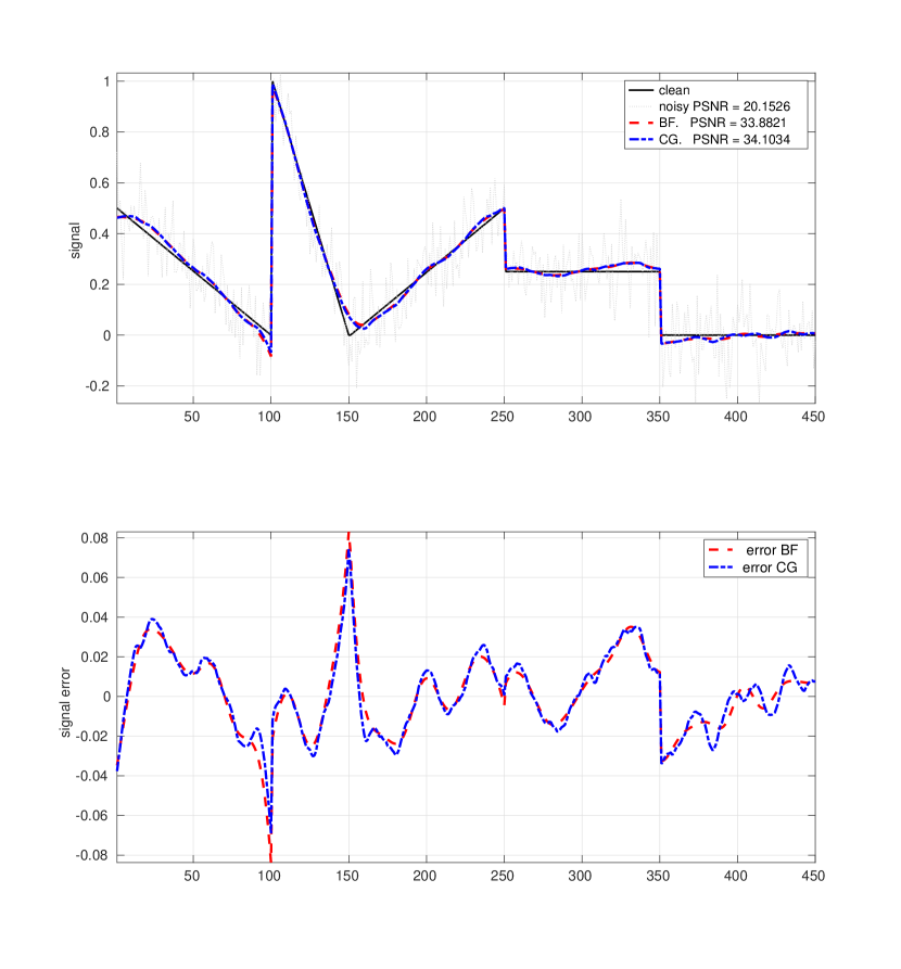
Figure 6: Edge-enhancing filtering.

The noise is additive Gaussian, and the noisy signal is displayed using grey dots. The nonzero weights are computed by (2) with $\sigma_{d}=0.5$ and $\sigma_{1}=0.1$ only for $j=i-1,\,i,\,i+1$, resulting in tridiagonal matrices $W$ and $L$. BF is self-guided, with $W$ and $L$ recomputed on every iteration using the current approximation $x_{k}$ to the final filtered signal $x_{m}$. CG-BF uses the fixed nonzero weights computed also by (2), but for the noiseless signal $y$ resulting in the fixed tridiagonal matrices $W_{y}$ and $L_{y}$. The number of iterations in BF, 100, and CG-BF, 15, is tuned to match the errors. Formula (2) puts ones on the main diagonal of $W$, thus for small positive or negative $w_{i\,i+1}=w_{i+1\,i}$ the matrix $D$ is well-conditioned.

Figure 5 demonstrates the traditional approach with nonnegative weighs. We observe, as discussed in Section III, flattening at the end points. Moreover, there is noticeable edge smoothing in all corners, due to a large noise and relatively small number of signal samples, despite of the use of the edge-preserving formula (2). We set tuned negative graph weights $-2\times 10^{-3}$, $-10^{-3}$, $-10^{-8}$ for $i=100,\,250$, and $350$ correspondingly, to obtain Figure 6, which shows dramatic improvements both in terms of PSNR and edge matching, compared to Figure 5.

VI Conclusion

The proposed novel technology of negative graph weights allows designing edge enhancing filters, as explained theoretically and shown numerically for a synthetic example. Our future work concerns determining the optimal negative weights, testing the concept for image filtering, and exploring its advantages in spectral data clustering using correlations.

References

- [1] CuongCao Pham, SynhVietUyen Ha, and JaeWook Jeon, “Adaptive guided image filtering for sharpness enhancement and noise reduction,” in Advances in Image and Video Technology, Yo-Sung Ho, Ed., vol. 7087 of Lecture Notes in Computer Science, pp. 323–334. Springer Berlin Heidelberg, 2012.
- [2] Haoxing Wang, Longquan Dai, and Xiaopeng Zhang, “Edge guided high order image smoothing,” in Pattern Recognition (ACPR), 2013 2nd IAPR Asian Conference on, Nov 2013, pp. 682–686.
- [3] Kaiming He, Jian Sun, and Xiaoou Tang, “Guided image filtering,” Pattern Analysis and Machine Intelligence, IEEE Transactions on, vol. 35, no. 6, pp. 1397–1409, June 2013.
- [4] Serena Morigi, Lothar Reichel, and Fiorella Sgallari, “An edge-preserving multilevel method for deblurring, denoising, and segmentation,” in Scale Space and Variational Methods in Computer Vision, Xue-Cheng Tai, Knut Mørken, Marius Lysaker, and Knut-Andreas Lie, Eds., vol. 5567 of Lecture Notes in Computer Science, pp. 426–438. Springer Berlin Heidelberg, 2009.
- [5] Donghui Chen, Misha E. Kilmer, and Per Christian Hansen, ““Plug-and-Play” edge-preserving regularization,” Electronic Transactions on Numerical Analysis (ETNA), vol. 41, no. 2, pp. 465–477, 2014.
- [6] Zhengguo Li, Jinghong Zheng, Zijian Zhu, Wei Yao, and Shiqian Wu, “Weighted guided image filtering,” Image Processing, IEEE Transactions on, vol. 24, no. 1, pp. 120–129, Jan 2015.
- [7] M. Elad, “On the origin of the bilateral filter and ways to improve it,” Image Processing, IEEE Transactions on, vol. 11, no. 10, pp. 1141–1151, Oct 2002.
- [8] F. Porikli, “Constant time o(1) bilateral filtering,” in Computer Vision and Pattern Recognition, 2008. CVPR 2008. IEEE Conference on, June 2008, pp. 1–8.
- [9] Yinxue Zhang, Xuemin Tian, and Peng Ren, “An adaptive bilateral filter based framework for image denoising,” Neurocomputing, vol. 140, no. 0, pp. 299 – 316, 2014.
- [10] P. Milanfar, “A tour of modern image filtering: new insights and methods, both practical and theoretical,” IEEE Signal Processing Magazine, vol. 30, no. 1, pp. 106–128, 2013, doi: 10.1109/MSP.2011.2179329.
- [11] Fan R. K. Chung, Spectral Graph Theory, American Mathematical Society, 1997.
- [12] A. Levin, D. Lischinski, and Y. Weiss, “A closed-form solution to natural image matting,” Pattern Analysis and Machine Intelligence, IEEE Transactions on, vol. 30, no. 2, pp. 228–242, Feb 2008.
- [13] Kaiming He, Jian Sun, and Xiaoou Tang, “Fast matting using large kernel matting Laplacian matrices,” in Computer Vision and Pattern Recognition (CVPR), 2010 IEEE Conference on, June 2010, pp. 2165–2172.
- [14] D. K. Hammond, L. Jacques, and P. Vandergheynst, “Image denoising with nonlocal spectral graph wavelets,” in Image Processing and Analysis with Graphs, O. Lezoray and L. Grady, Eds., pp. 207–236. CRC Press, 2012.
- [15] D.I. Shuman, S.K. Narang, P. Frossard, A. Ortega, and P. Vandergheynst, “The emerging field of signal processing on graphs: Extending high-dimensional data analysis to networks and other irregular domains,” Signal Processing Magazine, IEEE, vol. 30, no. 3, pp. 83–98, 2013.
- [16] S. K. Narang, A. Gadde, E. Sanou, and A. Ortega, “Localized iterative methods for interpolation in graph structured data,” in Signal and Information Processing (GlobalSip), 1st IEEE Global Conf., Dec. 2013.
- [17] A. Gadde, S. K. Narang, and A. Ortega, “Bilateral filter: Graph spectral interpretation and extensions,” ICIP 2013, October 2013.
- [18] D. Tian, A. Knyazev, H. Mansour, , and A. Vetro, “Chebyshev and conjugate gradient filters for graph image denoising,” in Proceedings of IEEE International Conference on Multimedia and Expo Workshops (ICMEW), Chengdu, 2014, pp. 1–6.
- [19] Jaakko Särelä and Harri Valpola, “Denoising source separation,” J. Mach. Learn. Res., vol. 6, pp. 233–272, Dec. 2005.
- [20] Sebastian Mika, Bernhard Schölkopf, Alex J. Smola, Klaus-Robert Müller, Matthias Scholz, and Gunnar Rätsch, “Kernel pca and de-noising in feature spaces,” in Advances in Neural Information Processing Systems 11, M.J. Kearns, S.A. Solla, and D.A. Cohn, Eds., pp. 536–542. MIT Press, 1999.
- [21] Luca Rossi, Andrea Torsello, and Edwin R. Hancock, “Unfolding kernel embeddings of graphs: Enhancing class separation through manifold learning,” Pattern Recognition, , no. 0, pp. –, 2015.
- [22] P. Perona and J. Malik, “Scale-space and edge detection using anisotropic diffusion,” in Proceedings of IEEE Computer Society Workshop on Computer Vision, Miami, FL, 1987, pp. 16–27.
- [23] P. Perona and J. Malik, “Scale-space and edge detection using anisotropic diffusion,” IEEE Transactions on Pattern Analysis and Machine Intelligence, vol. 12, no. 7, pp. 629–639, 1990, doi: 10.1109/34.56205.
- [24] F. Zhang and E. R. Hancock, “Graph spectral image smoothing using the heat kernel,” Pattern Recogn., vol. 41, no. 11, pp. 3328–3342, Nov. 2008.
- [25] M. R. Hestenes and E. Stiefel, “Methods of conjugate gradients for solving linear systems,” Journal of research of the National Bureau of Standards, vol. 49, pp. 409–436, 1952.
- [26] A. Greenbaum, Iterative Methods for Solving Linear Systems, SIAM, Philadelphia, PA, 1997, doi: 10.1137/1.9781611970937.
- [27] Pi Sheng Chang and Jr. Willson, A.N., “Analysis of conjugate gradient algorithms for adaptive filtering,” Signal Processing, IEEE Transactions on, vol. 48, no. 2, pp. 409–418, Feb 2000.
- [28] C. Tomasi and R. Manduchi, “Bilateral filtering for gray and color images,” in Proceeedings of IEEE International Conference on Computer Vision, Bombay, 1998, pp. 839–846, doi: 10.1109/ICCV.1998.710815.
- [29] S. Paris, P. Kornprobst, J. Tumblin, and F. Durand, “Bilateral filtering: Theory and applications,” Foundations and Trends in Computer Graphics, vol. 4, no. 1, pp. 1–73, 2009, doi: 10.1561/0600000020.
- [30] Jianbo Shi and Jitendra Malik, “Normalized cuts and image segmentation,” IEEE Trans. Pattern Anal. Mach. Intell., vol. 22, no. 8, pp. 888–905, Aug. 2000.
- [31] Andrew Y Ng, Michael I Jordan, Yair Weiss, et al., “On spectral clustering: Analysis and an algorithm,” Advances in neural information processing systems, vol. 2, pp. 849–856, 2002.
- [32] A. V. Knyazev, “Modern preconditioned eigensolvers for spectral image segmentation and graph bisection,” in Proceedings of the workshop Clustering Large Data Sets; Third IEEE International Conference on Data Mining (ICDM 2003), Boley, Dhillon, Ghosh, and Kogan, Eds., Melbourne, Florida, 2003, pp. 59–62, IEEE Computer Society.
- [33] Jinho Park, Moongu Jeon, and Witold Pedrycz, “Spectral clustering with physical intuition on spring–mass dynamics,” Journal of the Franklin Institute, vol. 351, no. 6, pp. 3245 – 3268, 2014.
- [34] Frédo Durand and Julie Dorsey, “Fast bilateral filtering for the display of high-dynamic-range images,” ACM Trans. Graph., vol. 21, no. 3, pp. 257–266, July 2002.