Prospects for Measuring the Positron Excess with the Cherenkov Telescope Array
Abstract:
The excess of positrons in cosmic rays above 10 GeV has been a puzzle since it was discovered. Possible interpretations of the excess have been suggested, including acceleration in a local supernova remnant or annihilation of dark matter particles. To discriminate between these scenarios, the positron fraction must be measured at higher energies. One technique to perform this measurement is using the Earth-Moon spectrometer: observing the deflection of positron and electron moon shadows by the Earth’s magnetic field. The measurement has been attempted by previous imaging atmospheric Cherenkov telescopes without success. The Cherenkov Telescope Array (CTA) will have unprecedented sensitivity and background rejection that could make this measurement successful for the first time. In addition, the possibility of using silicon photomultipliers in some of the CTA telescopes could greatly increase the feasibility of making observations near the moon. Estimates of the capabilities of CTA to measure the positron fraction using simulated observations of the moon shadow will be presented.
1 Introduction
Positrons can be created by interactions between cosmic rays and the insterstellar medium. Our knowledge of the cosmic ray spectrum and the interstellar environment allows us to predict the spectrum of positrons incident upon the Earth due to this secondary production of positrons. Since the 1970s there have been experimental hints in the measured positron fraction and the total electron and positron flux that the spectrum of positrons at Earth deviates from that expected from secondary production, indicating additional production of positrons [1]. The first definitive measurement showing that the positron fraction is rising at energies ¿1 GeV came from the PAMELA experiment in 2009 [2]. More recently, this result has been confirmed by the Fermi-LAT [3] and extended up to 500 GeV by the AMS-02 experiment [4].
There are several interpretations of the rising positron fraction at high energies which correspond to different sources of the positrons [5]. One example is the production of secondary positrons inside supernova remnants [6]. Such positrons would have a harder spectrum than those produced through interactions with the interstellar medium, and therefore could produce the anomaly in the positron fraction. Another possibility is the presence of a nearby object that is accelerating positrons such as a pulsar or microquasar. A third possibility is the production of electrons and positrons due to the annihilation or decay of dark matter particles. This is a very exciting idea but there are many models of dark matter. There is quite a bit of uncertainty in both the parameter space of dark matter and the astrophysical models but some distinguishing characteristics have been predicted. For example, an important clue is the exact shape of the positron fraction at high energies. If the positrons are due to dark matter, the positron spectrum should have a sharp cutoff at an energy determined by the dark matter mass, which is then smoothed by propagation effects. There must be a high energy limit for secondary positron acceleration in astrophysical sources as well, but the cutoff should be less sharp. To address this question, a measurement of the positron fraction beyond the energy reach of AMS-02 could be crucial (current publications report the electron flux up to 700 GeV and the positron flux up to 500 GeV).
The positron fraction can be measured at high energies using what is known as the Earth-Moon spectrometer. A fraction of cosmic rays that would have arrived at Earth are blocked by the moon creating a deficit in the distribution of cosmic-rays as observed from the Earth (a moon shadow). The subsequent deflection of the cosmic rays by Earth’s magnetic field as they travel from the moon to Earth causes the moon shadow to shift in different directions for positively and negatively charged particles. In a certain energy range, which depends somewhat on the local magnetic field, the particles are bent enough that the two shadows are fully separated but not so much that the shadows are smeared out over a large section of the sky so that the shadows are observable. By binning the events in energy, it should be possible to resolve the moon shadows of particles at different energies and therefore measure the spectrum of electrons and positrons. Imaging atmospheric Cherenkov telescopes (IACTs) are well suited for this measurement because of their good angular and energy resolution. The use of this technique to measure the positron fraction was first attempted with the ARTEMIS experiment, but the background conditions proved too challenging [7]. More recently, this measurement has been attempted with the MAGIC observatory which is an ongoing effort [8].
The measurement of the positron fraction using the Earth-Moon spectrometer is challenging for several reasons. IACTs are designed to be operated in low moonlight conditions because photomultiplier tubes (PMTs) are damaged by ambient light. This severely limits the ability to point the telescope to a location near the moon (as close as possible for the highest energy measurements). Observing during low moon phase is favorable, but observing is also only possible when the source is relatively high in the sky, which for the moon tends to be at high phase. This typically means that a few tens of hours are available for this observation per year. The ARTEMIS measurements were made using special filters designed to attenuate moonlight while allowing the Cherenkov light through, but the background light conditions were nonetheless challenging. The other principal background that complicates this measurement is protons. Generally, even after standard gamma-hadron separation cuts have been applied, the number of residual protons will still outnumber positrons of the same energy by an order of magnitude. Since protons and positrons have the same charge, they will be deflected nearly identically at ultrarelativistic energies, and therefore the positron moon shadow at a given energy will be hidden in a proton shadow at that same energy. Additional work must be done in data analysis to extract the positron signal from an observation of the positive shadow. Observation of the negative shadow, where electrons have a deficit and protons and positrons are distributed uniformly will give another handle on the proton contribution.
The Cherenkov Telescope Array (CTA) is a next-generation IACT which is currently in the planning and prototyping stage and scheduled to finish construction in 2020 [9]. CTA will have an array in both the North and South hemispheres and each array will consist of many tens of telescopes instead of two to five as in the current generation. Current plans for the southern array could feature over 100 telescopes spread over an area 3 km in diameter. By using three different telescope sizes, it will be able to cover a wide energy range, from a few tens of GeV to a few hundreds of TeV with an order of magnitude improvement in sensitivity over current IACTs. CTA will have a better chance of successfully measuring the positron fraction than any previously conceived IACT for several reasons beyond the overall increase in area and sensitivity. First, CTA will have a wide field of view, around for the medium-sized telescopes. This is critical for this study because observing the shadow at different angular separations away from the moon is equivalent to measuring different energies. A wider field of view means the flux can be determined in more energy bins in one pointing. More than one pointing may not be possible because as stated above, there will not be many hours available for the measurement (especially with the competition of many other exciting observing targets). Another reason CTA will be superior to previous IACTs for this measurement is that some of the camera designs feature silicon photomultipliers (SiPMs) rather than the traditional PMTs. All of the small-sized telescopes and some of the medium-sized telescopes are proposed to be instrumented with SiPMs, which are much more robust than PMTs and will not be damaged by the high moonlight conditions. The large number of telescopes in CTA makes it impractical to temporarily install filters, but the SiPMs will allow those telescopes to be pointed at or near the moon. There will be an increase in energy threshold for such observations, but no threat to the photodetectors. This has been proven by the FACT telescope, which has observed showers while tracking the full moon using a SiPM camera [10]. Finally, improvements in camera technology and a greater telescope multiplicity will allow for improved gamma-hadron separation, which will make the task of rejecting the large proton background easier. The remainder of this paper will describe the results of a proof-of-concept study to show the capabilities of CTA to measure the electron and positron spectra using simulations, with a focus on a method for the rejection of the proton background.
2 Models, Simulations, and Assumptions
To evaluate the capabilities of CTA to detect electrons and positrons, a model for the spectra of electrons and positrons at high energies was needed. In a recent paper by Mertsch and Sarkar, they present calculations based on the supernova remnant hypothesis of secondary positron acceleration [6]. They use recent data from AMS-02 to fix some of the free parameters of their model and extrapolate the spectra to high energies (as well as make predictions about other cosmic ray species). Within the remaining allowed variations in model parameters, there is the possibility that the positron fraction could rise to nearly 50% at a few TeV, making this model useful for studying the performance of our analysis method.
Next, it is necessary to simulate the response of CTA to particles with the above spectra. The number of each type of telescope has not been finalized, nor has the exact layout, but simulations of various array configurations have been carried out and the results published [11]. For this project, the array configuration designated as ‘2A’ from the second round of Monte Carlo production (i.e. Prod-2) was used, which consists of 4 Large-Sized Telescopes (LSTs), 24 Medium-Sized Telescopes (MSTs), and 37 Small-Sized Telescopes (SSTs). It is worth noting that the number of SSTs is likely to be considerably more than what is simulated here, while not all the MSTs will be instrumented with SiPMs. In addition, the level of night sky background in these simulations was fairly low, corresponding to the brightness of an extragalactic field with an integral intensity of 0.22/ns/sr/cm2 between 300 and 650 nm. Nevertheless, the simulation yields sufficiently reasonable quantities to begin this study. Using the resulting simulated effective area and residual protons as a function of energy, the expected rate of electrons, positrons, and protons in chosen energy bins can be calculated for any input spectrum.
To produce a simulated observation of the positive and negative moon shadows, we needed to model the deflection of the particles by the Earth’s magnetic field. The deflection will depend on the local magnetic field at the location of the array, which is still not known as of this writing. In the interest of comparing to existing studies, it was decided to create our simulations using an approximation previously used by the MAGIC collaboration for their site on La Palma, i.e. the deflection is ). This means the highest energy accessible with this measurement is 3 TeV, where the shadows would be displaced by , or 1 moon diameter. In this simulation a coordinate system is chosen such that the true moon location is at the origin and the magnetic deflection is along the x-axis. Then for each energy bin, the shadow covers a range of x-coordinates. There is also spread in both the x and y directions by factoring in the point spread function, which is larger for the residual protons than for the leptons (also obtained from simulation).
In our simulation, there are 9 energy bins extending from 100 GeV up to about 3 TeV (6 bins per decade). Each energy bin and shadow (one to the left of the moon and one to the right) is treated as a separate 100 hour observation with spatial boundaries corresponding to a rectangle which is 5 times the proton PSF away from the location of the moon shadows at either end of the energy bin. These simplifications were chosen to give a clear and complete image of the shadows to the analysis so it could be tested without worrying about edge effects, but plans for a more realistic simulation are outlined at the end of these proceedings. The expected number of electrons, positrons, and protons for the 100 hour duration and appropriate solid angle are thrown uniformly over the area. It is determined whether or not each one would have been blocked by the moon based on its deflection, and the PSF smearing is applied. In this way a simulated observation of the moon shadows in each bin is generated consisting of a uniform flux with a deficit of the appropriate shape, location, and depth. It is assumed that the measurement is done on an area of the sky that is not near any source of gamma rays. The diffuse gamma ray background is at least two orders of magnitude lower than the flux of cosmic rays, so only electrons, positrons, and protons are simulated.
3 Template Method
As stated above, a significant challenge of this measurement is removing the residual protons. Most protons can be removed from the data by analysis of the shape of the shower in the image. CTA will have a higher efficiency in this process than any previous IACT. However, some proton showers are more difficult to reject due to the stochastic nature of the shower development. For example, a proton shower can create an electromagnetic subshower far from the rest of the shower which would then be indistinguishable from a shower resulting from a gamma ray, electron, or positron. Due to the overwhelming prevalence of protons in cosmic rays, these residual protons will still outnumber positrons by an order of magnitude in CTA data, according to our simulations.
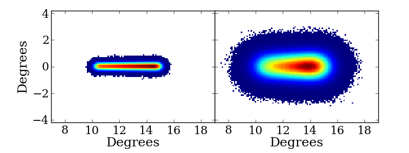
At ultrarelativistic energies, the deflection of positrons and protons is nearly identical so the shadows for both particles lie on top of each other. However, the proton shadow is much wider because the PSF for protons is larger. The template method is a technique which exploits this fact to remove the protons. Two-dimensional templates for the shapes of the shadows of different particles are simulated by assuming the spectra can be approximated as power laws within an energy bin. Then particles are thrown from that power law, deflected, and smeared with the appropriate PSF as above. The templates are broken up into small pixels () so that the shapes of the shadows can be accurately distinguished. Different power law indices can be simulated and fit as hypotheses. The normalizations of the three components are fit to the data using a minimization which gives as output the fluxes of each particle and associated errors. The two shadows are fit simultaneously with the appropriate templates used for each shadow. For example, for the ”positive” shadow, the electrons are fit using a flat template, the protons are fit using the wider deficit template, and the positrons are fit using the narrower deficit template. The template used for the positron deficit on one side of the moon and the electron deficit, while similar in shape, must be different because the two species will generally have different power law indices in a given bin, which changes the depth of the deficit. Some examples of templates are shown in Figs. 1 and 2.

To improve the fit, the total electron-positron spectrum can be used as a prior. The prior could be based on the spectrum derived from CTA or a previous measurement. For example, the H.E.S.S. experiment reported a measurement of the total spectrum with 30% systematic errors [12]. Since the systematic errors are mostly due to uncertainties of hadronic interaction models, it is unclear how much these will be reduced by the time CTA makes a measurement. For this simulation, the prior is a ”measurement” of the sum of the electron and positron input spectra with a 30% error.
Let , , and be the normalizations of the electron, positron, and proton components, respectively. Let be the value in the th pixel of the flat template corresponding to a uniform intensity for each particle over the field of view, and let , , and be the value in the th pixel of the templates for the positron, proton, and electron deficits, respectively. Then the model for the positive shadow is:
| (1) |
and the model for the negative shadow is:
| (2) |
If and are the values of the th pixels in the data (or in this case simulation) for the two shadows, is a prior measurement of the total electron and positron spectrum converted into the appropriate units, and is the error of that measurement, then the quantity to be minimized is:
| (3) |
which can be done with a simple matrix inversion.
4 Results
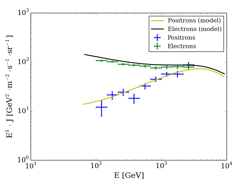
The results of this simulation can be seen in Fig. 3. From this plot it is evident that there seems to be a systematic shift in the reconstructed electron spectrum. The cause of this shift is under investigation. However, the method generally seems to be successful for reconstructing the input spectra. The input spectra are ”optimistic” in the sense that the positron fraction is high at TeV energies, but nonetheless the good performance particularly in the region beyond the current reach of AMS-02 is encouraging.
5 Future Work
There are several ways to improve upon the work done so far. First, the choice of the field of view for the above work was quite artificial. A round 8∘ field of view which is fixed on the sky for all energy bins would be more realistic and would reveal more about the range of energies that could actually be measured by a CTA observation. Fortunately, the most interesting energy bins are the highest energies, for which it will be easier to fit both shadows in a single field of view. More study is needed to determine whether it might be more optimal to divide the observations between two pointings to capture both shadows over a wider energy range. As can be seen from the example templates, it may be unreasonable to extend the measurement down to 100 GeV, as the shadows could extend to 15∘ from the moon. However, at that energy, the positron fraction has already been measured well by AMS-02.
In fact, there is another reason why low energies may not be accessible which is the high night sky background. Although the SiPM cameras will not be damaged by pointing the telescope close to the moon, the increase in the night sky background rate within the field of view will degrade the reconstruction performance somewhat and increase the trigger energy threshold. Detailed simulations have not yet been done with such high background light conditions. Future studies with more background light and an updated estimation of the baseline array layout will help to more accurately characterize the performance, but again, losing the lowest energies will not be so important.
Finally, the next pass of this study will contain a more accurate treatment of the proton energy. It is true that protons and positrons of the same true energy are deflected by the same amount in the magnetic field, but the events will be binned in reconstructed energy. In particular, the proton showers which are misreconstructed as electromagnetic showers tend to be due to images of a subshower, and therefore the reconstructed energy is on average about a third of the true proton energy (with significant spread, again due to the stochastic nature of the shower development). This offset has not been taken into account in this study so far. Doing this properly could significantly improve the ability to distinguish protons from positrons because now the deficits in a reconstructed energy bin will no longer be on top of each other. In fact, after taking these effects into account, the protons may be better modeled with a flat distribution rather than with a wide deficit.
With all of the above improvements, this proof-of-concept study will be developed into an improved estimate of the sensitivity of CTA to the positron fraction.
We gratefully acknowledge support from the agencies and organizations listed in this page: http://www.cta-observatory.org/?q=node/22.
References
-
[1]
B. Agrinier et al., Lett. Nuovo Cimiento 1 (1969) 1.
A. Buffington et al., Ap. J. 199 (1975) 669.
D. Müller and K. Tang, Ap. J. 312 (1987) 183.
R. L. Golden et al., Astron. and Astrophys. 188 (1987) 145.
R. L. Golden et al., Ap. J. 436 (1994) 769.
S. Barwick et al., Phys. Rev. Lett. 75 (1995).
J. Chang et al., Nature 456 (2008) 362.
A. Abdo et al., Phys. Rev. Lett. 102, 181101 (2009). - [2] O. Adriani et al., Nature 458 (2009).
- [3] M. Ackermann et al., Phys. Rev. Lett. 108, 011103 (2012).
- [4] L. Accardo et al., Phys Rev. Lett. 113, 121101 (2014).
-
[5]
P. Serpico, Astropart. Phys. 39 (2012).
Y. Fan, B. Zhang, and J. Chang, Int. Jour. of Mod. Phys. D 19 (2010) 13. - [6] P. Mertsch and S. Sarkar, Phys. Rev. D 90, 061301(R) (2014).
- [7] D. Pomarede et al., Astropart. Phys. 14 (2001) 287.
- [8] P. Colin et al., Proc. of 32nd ICRC (2011).
- [9] B. Acharya et al., Astropart. Phys. 43 (2013).
- [10] M. Knoetig et al., Proceedings of 33rd ICRC (2013) astro-ph:1307.6116.
- [11] K. Bernlöhr et al., Astropart. Phys. 43 (2013).
- [12] F. Aharonian et al., Astronomy and Astrophysics 508 (2009).