A Jacobian generalization of the pseudo Nambu–Goldstone boson potential

Abstract

We enlarge the classes of inflaton and quintessence fields by generalizing the pseudo Nambu–Goldstone boson potential by means of elliptic Jacobian functions, which are characterized by a parameter $k$. We use such a generalization to implement an inflationary era and a late acceleration of the universe. As an inflationary model the Jacobian generalization leads us to a number of e-foldings and a primordial spectrum of perturbations compatible with the Planck collaboration 2015. As a quintessence model, a study of the evolution of its equation of state (EoS) and its $w^{\prime}$–$w$ plane helps us to classify it as a thawing model. This allows us to consider analytical approximations for the EoS recently discovered for thawing quintessence. By using JLA Supernovae Ia and Hubble parameter $H(z)$ data sets, we perform an observational analysis of the viability of the model as quintessence.

PACS numbers:

1 Introduction

Scalar fields are widely used to endeavor to explain some aspects of the modern cosmology, in particular, the inflationary epoch in early times and the recent acceleration of the universe. Mechanisms for inflation and recent acceleration are not so different. The main difference is that non-relativistic matter cannot be ignored in recent times. Moreover, the energy scale of the quintessence potentials needs to be much smaller than the inflationary ones.

Inflation is a period preceding the standard cosmology where the evolution of the universe can be described by a scalar field, the inflaton. It was proposed to solve the horizon and the flatness problems of the standard model, as well as provide the mechanism to generate the seeds for the formation of structures and anisotropies of the cosmic microwave background (CMB). During the inflationary period, the universe accelerates its expansion to an almost exponential rate, cooling and smoothing the spatial structure. Furthermore, inflation predicts fluctuations with an almost scale invariant spectrum which has been confirmed by recent CMB data [1, 2]. To connect with the standard cosmological periods dominated by radiation and matter, it is necessary to add a period of reheating. The usual mechanism can also be preceded by a more efficient phase known as preheating [3, 4, 5, 6].

On the other hand, several cosmological experiments have demostrated the existence of a phase of accelerated expansion in current times [1, 2, 7, 8, 9]. This leads us to one of the most challenging problems in cosmology: the nature of dark energy. So far, the most sucessful dark energy candidate is the cosmological constant $\Lambda$. However, this model apparently has shortcomings such as discrepancy between the value of the vacuum energy obtained through observations and its estimated theoretical value, or even the coincidence problem [10, 11, 12]. Thus, in recent years, alternatives to solve these problems have been sought. Alternatives to the $\Lambda$CDM model can be divided into two groups. In the first group, general relativity is modified to obtain late acceleration without exotic components (see for example Refs. modifies-modifies3). The second group is related to the existence of an exotic fluid with negative pressure such as Chaplygin gas, $k$-essence, quintessence and others [16, 17, 18, 19, 20, 21, 22, 23]. In all these alternatives the dark energy equation of state (EoS) changes dynamically with time differently from the $\Lambda$CDM, the EoS of which is constant and equals $-1$. In the context of quintessence, a canonical scalar field $\phi$ minimally coupled to gravity is used as a dark energy model. The field $\phi$ varying slowly along a potential $V(\phi)$ can lead to observational results very similar to the cosmological constant (for a review see for example Refs.  Copeland2006,Tsujikawa2013).

One of the most interesting models for inflation and dark energy is an ultra-light pseudo Nambu–Goldstone boson (pNGB) which is still relaxing to its vacuum state. From the viewpoint of quantum field theory, pNGB models are the simplest way to have a naturally ultra-low mass, spin-0 particles and hence, perhaps the most natural candidate for a minimally coupled scalar field presently existing. The pNGB effective potential is given by

$$V(\phi)=\mu^{4}\,\left[1\pm\cos\left(\frac{\phi}{f}\right)\right],$$ (1)

where $f\sim m_{p}\simeq 10^{19}\,\textrm{GeV}$ is the Planck scale representing the spontaneous breaking scale, and $\mu$ is related to the explicit global symmetry breaking scale. Note that $f\rightarrow\infty$ corresponds to the exact shift symmetric constant potential. pNGBs were first proposed in the context of natural inflation [26], and then they were subsequently extended for the case of dark energy [27]. Also, a semiclassical calculation of particle production by a Nambu–Goldstone boson is performed in Ref. Dolgov.

On the other hand, analytical integration of the motion equations, in context of both inflation and quintessence, admits as solutions potentials related to hyperbolic functions [31, 32, 30, 29, 33]. In fact, some of these potentials can be considered as hyperbolic extensions of (1). Additionally, elliptic functions have been considered to study some inflationary aspects [34] and it was recently shown, in context of Hamilton-Jacobi method, that solutions related to the inflationary potential can be expressed in terms of elliptic functions [35, 36]. Furthermore, in recent times, Friedman–Robertson–Walker universe (FRW) containing a mixture of perfect fluids and a quintessence escalar field, admits as solutions for the potential, some especial cases of elliptic functions [33]. Within this context and keeping in mind that trigonometric and hyperbolic functions are particular cases of Jacobi’s elliptic functions, we propose, in some sense, a unified treatment of all of these potentials. For this reason we generalize Eq. (1) in an elliptic version by means of Jacobi functions, and we use it to implement an inflationary era and a late acceleration of the universe. Such a generalization owns a shift symmetry, like the pNGB potential, important to solve the two reasons that render challenging to find a natural candidate for quintessence field in particle physics. The first reason is related to the violation of the flatness condition (see for example Ref. Kolda1998), while the second is related to the fact that an ultra-light field would carry a fifth force, typically of gravitational strength (see for example Refs. Carroll1998,Chiba1999). In this work we shall limit ourselves to the case of the FRW homogeneous and isotropic metric with null curvature.

This paper is organized as follows: in Section 2 we present the generalized potential which can be expressed in terms of elliptic functions. In Section 3 an inflationary model based on the generalized potential is presented. We provide the general solutions and the expressions for the relevant cosmological parameters and then we study the viability of the model in the context of recent data from the Planck collaboration 2015 [2]. In Section 4 we study the generalized potential as a dark energy model, i.e., as a quintessence model. We perform the study of the evolution of its EoS and of the phase space $w^{\prime}-w$ . Finally, we perform observational tests to investigate the viability of quintessence models based on the Jacobian generalization. In section 5 we present our conclusions and final remarks.

2 Jacobian pseudo Nambu–Goldstone boson

Recalling that trigonometric functions are special cases of elliptic functions, we proceed to generalize the effective potential (1) in a simple way:

$$V(\phi,\,k)=\mu^{4}\,\left[1+\textrm{cn}\left(\frac{\phi}{f}\right)\right],$$ (2)

where $\textrm{cn}(x)\equiv\textrm{cn}(x|\,k)$ is the Jacobi’s elliptic cosine function, and $k$ is the modulus of the elliptic function. Note that the original pNGB potential is recovered by making $k=0$. We will refer to potential (2) as Jacobian pseudo Nambu–Goldstone boson (JpNGB) effective potential. In FIG. 1 the effective potential (2) is plotted for different values of the modulus $k$ and in the Appendix some properties of the Jacobi’s elliptic function are presented. Without loss of generality, we will consider that $\mu$ and $f$ possess the same physical meaning as in the pNGB scheme.

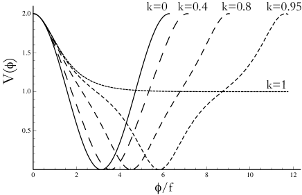
Figure 1: Plot of the Jacobian pseudo Nambu–Goldstone boson effective potential $V$ as a function of the dimensionless scalar field $\varphi=\phi/f$ for different values of the modulus $k$. Clearly, the hyperbolic limit $k=1$ does not allow inflation to end because the inflaton rolls eternally.

Alternatively, we mention that Higaki & Takahashi [34] have recently studied the case with a minus sign in the potential (2) calling this model the Cnoidal inflation. Specifically, they have shown that this model predicts values of the spectral index and the tensor–to–scalar ratio that interpolates from natural inflation to exponential inflation such as $R^{2}$–or Higgs inflation and brane inflation. In the next section we will use potential (2) to implement an inflationary epoch in the early universe and we will study its concordance with observational data of the Planck satellite.

3 JpNGB as a inflaton field

In the inflationary regime, the dynamical evolution of the JpNGB field is described by the Klein–Gordon equation

$$\ddot{\phi}+(3H+\Gamma)\dot{\phi}+V_{,\phi}=0,$$ (3)

where $\Gamma$ is the decay width of the inflation, the dot indicates the derivative with respect to time, $H=\dot{a}/a$ and $V_{,\phi}$ represents the derivative of the potential with respect to $\phi$. Note that in the temperature range $\mu\lesssim T\lesssim f$, the JpNGB potential is dynamically irrelevant because the term $V_{,\phi}$ is negligible when compared to the Hubble damping term. Therefore, in this temperature range, aside from the smoothing of spatial gradients in $\phi$, the field does not evolve. For temperatures $T\lesssim f$, the global symmetry is spontaneously broken, and the field $\phi$ describes the phase degree of freedom around the bottom of the potential. Since $\phi$ thermally decouples at a temperature $T\sim f^{2}/m_{p}\sim f$ we assume it is initially laid down at random between 0 and $Pf$ in different causally connected regions, where $P$ is the period of the elliptic function.

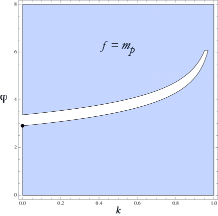
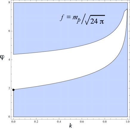
Figure 2: Plots for the condition (7) in the $\varphi$–$k$ plane for two values of $f$. The validity of inequality (7) is represented by the grey region of each graph and the boundary corresponds to the value of dimensionless scalar field $\varphi$ at the end of inflation, $\varphi_{e}$. Also, the value reported by Freese et al. [26] for $k=0$, $\varphi_{e}^{0}$, is represented by a dot. Top panel: $f=m_{p}$ and $\varphi_{e}^{0}=2.98$; Bottom panel: $f=m_{p}/\sqrt{24\pi}$ and $\varphi_{e}^{0}=1.9$.

Finally, at temperatures $T\lesssim\mu$, in regions of the universe with $\phi$ initially near the top of the potential, the field starts to roll slowly down the hill toward the minimum. In those regions, the energy density of the universe is quickly dominated by the vacuum contribution $[V(\phi)\simeq 2\mu^{4}\gtrsim p_{rad}\sim T]$, and the universe expands exponentially. The slow-roll (SR) regime occurs when the motion of the field is overdamped, so $\ddot{\phi}\ll 3H\dot{\phi}$ and $\Gamma\ll H$, and therefore two conditions are met:

$$|V_{,\phi\phi}(\phi|)|\lesssim 9H^{2},$$ (4)

and

$$\left|\frac{V_{,\phi}(\phi)}{V(\phi)}\right|\lesssim\frac{\sqrt{48\pi}}{m_{p}},$$ (5)

which, using Eq. (2) and defining the dimensionless scalar field $\varphi=\phi/f$, leads to

$$\sqrt{\frac{2\,\textrm{cn}\,\varphi\,|\textrm{dn}^{2}\,\varphi-k^{2}\textrm{sn}^{2}\,\varphi|}{1+\textrm{cn}\,\varphi}}\lesssim\frac{\sqrt{48\pi}f}{m_{p}},$$ (6)

and

$$\frac{|\textrm{dn}\,\varphi\,\textrm{sn}\,\varphi|}{1+\textrm{cn}\,\varphi}\lesssim\frac{\sqrt{48\pi}f}{m_{p}},$$ (7)

respectively (see definitions and relations of Jacobi’s elliptic functions in the Appendix). Obviously, the SR regime ends when one of inequalities (6) or (7) is violated. This fact occurs when $\phi$ reaches a value $\phi_{e}$ which is evaluated for $f=m_{p}$ and $f=m_{p}/\sqrt{24\pi}$ in FIG. 2. Note the consistency between our results and those found previously by Freese, Frieman & Olinto [26] using k=0, i. e. $\varphi_{e}^{0}=2.98$ for $f=m_{p}$ and $\varphi_{e}^{0}=1.9$ for $f=m_{p}/\sqrt{24\pi}$.

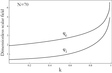
Figure 3: Numerical solution for the initial value $\varphi_{i}$ and final value $\varphi_{e}$ of the inflaton as a function of the modulus $k$ using $N=70$ and $f=m_{p}/\sqrt{24\pi}$.

Now let us calculate the values of the inflaton related to the number of e-folds required to generate the seeds for the creation of the large scale structures. As is well known, the number of e-folds of physical expansion that occur in the inflationary stage is given by

$$N(\phi) = -\frac{8\pi}{m_{p}^{2}}\int_{\phi}^{\phi_{e}}\frac{V}{V_{,\phi}}d\phi$$ (8)

$$= \frac{8\pi f^{2}}{m_{p}^{2}}\ln\left(\frac{\textrm{ds}\,\varphi}{\textrm{ds}\,\varphi_{e}}\sqrt{\frac{1-\textrm{cn}\,\varphi_{e}}{1+\textrm{cn}\,\varphi_{e}}\frac{1+\textrm{cn}\,\varphi}{1-\textrm{cn}\,\varphi}}\,e^{\Phi-\Phi_{e}}\right),$$

where

$$\Phi\equiv\sqrt{\frac{k}{k^{\prime}}}\,\arctan\left(\sqrt{\frac{k}{k^{\prime}}}\,\textrm{cn}\,\varphi\right),$$ (9)

and $k^{\prime}=1-k$ is the complementary modulus. Therefore, knowing the value of $\phi_{e}$ from Eq. (7) the initial value of the inflaton $\phi_{i}$ can be calculated, imposing a value on $N$, for example, $N(\phi_{i})=70$. In FIG. 3 we show the initial $\varphi_{i}$ and final $\varphi_{e}$ values of inflaton calculated using Eq. (8) and $f=m_{p}/\sqrt{24\pi}$ as a function of the modulus $k$. Our results indicate that for any value of $k$, the inflaton with a JpNGB effective potential is compatible with 70 e-folds. We have checked for values of $N(\phi_{i})$ between 60 and 70 and have found that the compatibility is maintained.

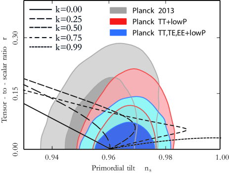
Figure 4: Plot of the tensor–to–scalar parameter $r$ as a function of the scalar spectral index $n_{s}$ for the Jacobian pseudo Nambu–Goldstone Bosons potential for $f=m_{p}/\sqrt{24\pi}$. The marginalized joint $68\%$ and $95\%$ confidence level regions using Planck TT + low P, Planck TT, TE, EE + low P and Planck 2013 data release with $\widehat{\rm{k}}=0.05h$ Mpc^-1 are shown [2].

In the inflationary scenario, the quantum fluctuations are relevant because they generate two important types of perturbations: density perturbations (arising from quantum fluctuations in the scalar field, together with the corresponding scalar metric perturbation), and relic gravitational waves (which are tensor metric fluctuations). The former is sensitive to gravitational instability and leads to structures formation, while the latter predicts a stochastic background of relic gravitational waves. Scalar perturbations produce a power spectrum characterized by the scalar spectral index $n_{s}$ while tensorial perturbations produce a power spectrum characterized by the gravitational wave spectral index $n_{T}$. In inflationary models it is common to define the tensor–to–scalar amplitude $r=\frac{P_{T}}{P_{R}}$, where $P_{T}$ and $P_{R}$ are amplitudes of the tensor and scalar power spectrum respectively.

The spectral index $n_{s}$ and the tensor–to–scalar amplitude ratio $r$ are written in terms of the slow–roll parameters,

$$\epsilon_{V} = \frac{m_{p}^{2}}{16\pi}\left(\frac{V_{,\phi}}{V}\right)^{2}=\frac{m_{p}^{2}}{16\pi f^{2}}\,\frac{\textrm{dn}^{2}\,\varphi\,\textrm{sn}^{2}\,\varphi}{(1+\textrm{cn}\,\varphi)^{2}}$$ (10)

$$\eta_{V} = \frac{m_{p}^{2}}{8\pi}\left(\frac{V_{,\phi\phi}}{V}\right)=\frac{m_{p}^{2}}{16\pi f^{2}}\,\frac{\textrm{cn}\,\varphi\,(2\,k\,\textrm{sn}^{2}\,\varphi-1)}{1+\textrm{cn}\,\varphi},$$ (11)

the spectral index and the tensor–to–scalar ratio are given by

$$n_{s} \simeq 1+2\,\eta_{V}-6\,\epsilon_{V}$$ (12)

$$= 1-\frac{3m_{p}^{2}}{8\pi f^{2}}\,\frac{\textrm{dn}^{2}\,\varphi\,\textrm{sn}^{2}\,\varphi}{(1+\textrm{cn}\,\varphi)^{2}}+\frac{m_{p}^{2}}{4\pi f^{2}}\,\frac{\textrm{cn}\,\varphi\,(2\,k\,\textrm{sn}^{2}\,\varphi-1)}{1+\textrm{cn}\,\varphi},$$

$$r \simeq 16\,\epsilon_{V}=\frac{m_{p}^{2}}{\pi f^{2}}\,\frac{\textrm{dn}^{2}\,\varphi\,\textrm{sn}^{2}\,\varphi}{(1+\textrm{cn}\,\varphi)^{2}}.$$ (13)

Therefore, using $n_{s}$ and $r$, it is possible to obtain a direct comparison of our results with the Planck collaboration data sets, which is shown in Figure 4. Based on such comparisons, we may say that a description of the inflationary universe model in terms of a JpNGB effective potential could quite well accommodate the data recently released by the Planck mission [2]. However, potentials with $k\sim 1$ are not viable because the inflaton rolls eternally.

4 JpNGB as dark energy

It is well known that a canonical scalar field $\phi$, called quintessence, varying slowly along one potential $V(\phi)$ can lead to observational results very similar to the cosmological constant and would explain the late acceleration of the universe (for a review see for example Ref. Tsujikawa2013). However, two reasons render it challenging to find a natural candidate for $\phi$ in particle physics. The first is related to the violation of the flatness condition [45], while the second is related to the fact that an ultra-light field would carry a fifth force, typically of gravitational strength [46, 47]. These problems can be solved by means of a potential which has a shift symmetry, as the pNGB potential [27].

The fact that potential (2), which is a generalization of pNGB, is a periodic function and therefore has a shift symmetry motivates us regarding the possibility of using it in order to construct a viable quintessence model. Thus we exploit its dynamic behavior when it is used to explain accelerated expansion in late times.

We start by considering the general motion equations in the case where the universe is dominated by a pressureless matter and a quintessence field. In the context of a homogeneous and isotropic Friedmann-Robertson-Walker universe, with null curvature and in the case where non-relativistic matter is not interacting with the quintessence field we have

$$\ddot{\phi}+3H\dot{\phi}+V_{,\phi}=0$$ (14)

$$\dot{\rho}_{m}+3H\rho_{m}=0$$ (15)

$$\dot{\rho}_{\phi}+3H(\rho_{\phi}+p_{\phi})=0$$ (16)

$$3H^{2}m_{P}^{2}=\rho_{m}+\rho_{\phi}\,.$$ (17)

where $\rho_{\phi}=\frac{1}{2}\dot{\phi}+V(\phi)$ and $p_{\phi}=\frac{1}{2}\dot{\phi}-V(\phi)$ are the density and pressure of the quintessence field respectively, and $w=p_{\phi}/\rho_{\phi}$ is the EoS of dark energy and subindex $m$ indicates matter. From (14)-(17) equations for $w$ and $\Omega_{\phi}=\rho_{\phi}/\rho_{crit}$, where $\rho_{crit}=3H_{0}^{2}m^{2}_{p}$ can be written (see for example Refs.  Dutta2008,Scherrer2008)

$$w^{\prime}=(1-w)\left[-3(1+w)+\lambda\sqrt{3(1+w)\Omega_{\phi}}\right]$$ (18)

$$\Omega^{\prime}_{\phi}=-3w\Omega_{\phi}(1-\Omega_{\phi})\,.$$ (19)

Additionally, one equation for the auxiliary variable $\lambda=-m_{p}V_{,\phi}/V$ is found

$$\lambda^{\prime}=-\sqrt{3(1+w)\Omega_{\phi}}\lambda^{2}(\widetilde{\Gamma}-1)\,,$$ (20)

where $\widetilde{\Gamma}=V_{,\phi\phi}\,V/V_{,\phi}^{2}$ and ^′ indicates derivative with respect to $\ln a$. Thus, given a potential $V$, $\widetilde{\Gamma}$ is known and the system (18)-(20) is completely determined. For example, for the exponential potential $\widetilde{\Gamma}=1$ and $\lambda$ is a constant and for pNGB potential $\tilde{\Gamma}=(\lambda^{2}-1)/2\lambda^{2}$. For our case $\tilde{\Gamma}$ has a more general dependence of $\lambda$ and we will find it numerically.

Recently, it was shown that quintessence models can be approximately separated into two classes, depending on the acceleration or deceleration of the field as it evolves down its potential towards to a zero minimum [44]. Such groups are called thawing and freezing quintessence and they behave quite differently. Models where the field is nearly frozen away from the minimum of the potential due to large Hubble dumping during the early cosmological era and starts to evolve towards the minimum recently are called thawing. Models where the field initially rolls towards its potential minimum and has only recently gradually slow down are called freezing [44]. Examples of the first group are the exponential and pNBG potentials [27, 49, 50, 51, 52, 53] and examples of the second group are the inverse power law potentials [54, 55, 56, 57]. In the next subsection we will show that our generalization belongs to the thawing group.

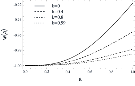
Figure 5: Evolution of EoS $w$ as a function of scale factor $a$ for different values of the parameter $k$ but same initial conditions. The case $k=0$ represents pNGB potential.

4.1 JpNGB as a thawing quintessence

As noted above, in thawing quintessence models, the field is initially frozen in early times and then as $H$ increases the field rolls down the potential. This means that at early times the EoS is $w\approx-1$ but grows less negative with time where $w^{\prime}>0$. Since we are generalizing the quintessence potential by means of (2), we are interested in knowing if such thawing behavior appears in this particular case.

In order to search the thawing characteristic we solve numerically the system (18)-(20) with same initial conditions and for different values of $k$-parameter. Results are shown in Figures (5) and (6). In FIG. (5) the evolution of the EoS as a function of scale factor $a$ is presented. For all cases we have used the same conditions: $f/m_{p}=0.9$ and $\phi_{i}/f=1.5$. As we can see, the same initial conditions lead us to different evolutions of EoS for each $k$. This opens the possibility of discriminating between different members of the family potentials (2) using observational data. In all cases $w$ is close to $-1$ for early times but begins to evolve for late times. Of course $k=0$ represents pNGB potential. We can note also that in the past, models with potential (2) are indistinguishable from the pNGB model and differences between them appear only recently. Additionally, it can be seen that the evolution of $w$ is slower for higher values of $k$.

In FIG. (6) we plot the behavior of the model on the dynamical phase space $w^{\prime}-w$ for different values of $k$ and for the same initial conditions. The upper shadowed area represents the thawing region $1+w\lesssim w^{\prime}<3(1+w)$ and the lower shadowed area represents the freezing region $0.2w(1+w)\lesssim w^{\prime}<3w(1+w)$ [44]. The values used in FIG.(6) are $f/m_{p}=1.1$ and $\phi_{i}/f=1.5$. Note that in all cases, curves are inside the thawing region and we can thus infer that JpNGB has thawing quintessence features. We have checked for a wide range of initial conditions ($0.6<\phi_{i}/f<2.5$) and $k$-parameters ($0<k<1$) and such thawing features are maintained. Thus we would expect that thawing features are always maintained.

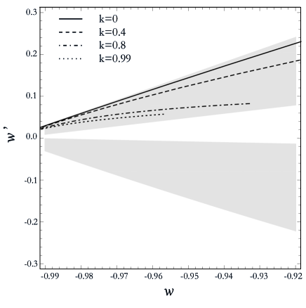
Figure 6: Plane representing the dynamical space phase $w^{\prime}-w$ and curves for JpNGB effective potential for different values of the modulus $k$. The upper shadowed area is the thawing region $1+w\lesssim w^{\prime}<3(1+w)$ and the lower shadowed area represents freezing region $0.2w(1+w)\lesssim w^{\prime}<3w(1+w)$.

Interestingly, for models having freezing and thawing properties an approximation of $w$ can be known analytically. In Refs.  Dutta2008,Chiba2009b the equations of motion (14) were solved in the limit when $w$ is close to $-1$ and an approximated EoS as a function of the scale factor was found when $|w+1|\ll 1$. The former condition is ensured if conditions of slow roll thawing quintessence $\frac{V^{\prime 2}}{6H^{2}V}\ll 1$ and $\frac{V^{\prime\prime}}{3H^{2}}\ll 1$ [58], in the case where both matter and a scalar field contribute to the density are satisfied. Such approximation gives us (see Refs. Dutta2008,Chiba2009b for details)

$$w(a)=-1+(1+w_{0})a^{3(K-1)}\times$$

$$\left(\frac{(K-F(a))(F(a)+1)^{K}+(K+F(a))(F(a)-1)^{K}}{(K-\Omega^{-1/2}_{\phi 0})(\Omega^{-1/2}_{\phi 0}+1)^{K}+(K+\Omega^{-1/2}_{\phi 0})(\Omega^{-1/2}_{\phi 0}-1)^{K}}\right)^{2}$$ (21)

where $w_{0}$ is the EoS in the current time and $K$ measures the potential curvature and it is

$$K=\sqrt{1-\frac{4M^{2}_{p}}{3}\frac{V_{,\phi\phi}(\phi_{i})}{V(\phi_{i})}}\,,$$ (22)

with $\phi_{i}$ being the initial value for $\phi$ and function $F(a)$ has the form

$$F(a)=\sqrt{1-(\Omega^{-1}_{\phi 0}-1)a^{-3}}\,.$$ (23)

Such approximation was found by means of a Taylor expansion around $\phi_{i}$ [58] and comparisons with other approximations like Chevallier-Polarski-Linde [63] and Crittenden [64] were performed in Ref. Chiba2009b. As shown in Refs. Dutta2008,Chiba2009b, numerical solutions are in excellent agreement with the approximate $w$ for several quintessence models including pNGB. We made the same comparison between exact and approximated EoS for JpNGB quintessence models. Results are presented in FIG.7 for different values of $k$. We have used the following values (i) $k=0.4$ $f/m_{p}=2$, $\phi_{i}/f=3$ ($K=1.6$); (ii) $k=0.8$, $f/m_{p}=2$ and $\phi_{i}/f=4$ ($K=1.6$) and (iii) $k=0.99$, $f/m_{p}=2$ and $\phi_{i}/f=6.6$ ($K=1.1$). In all figures, continuous curves correspond to an approximate solution (Eq,(4.1)) and dashed curves represent exact numerical solutions of the system (18)–(20).

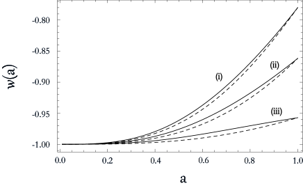
Figure 7: Evolution of the EoS as a function of $a$ using exact and approximate solutions. Dashed curves represent exact numerical solutions while continuous curves represent approximate solutions.

In order to evaluate the relative difference between exact and approximate solutions, the relative error ($|\delta w/w|$) was constructed for the curves in FIG.(7). Results are presented in FIG. (8). Note that in all cases the error is $\lesssim 0.9\%$, which is in agreement with relative errors for other quintessence models [58]. We have examined several cases by varying initial conditions, $k$ parameter, etc. and in all of them the highest relative error was $\sim 1\%$. As a conclusion, Eq. (4.1) gives a good approximate solution of EoS for our generalized model. Parametrization (4.1) lead us to $\Omega_{\phi 0}$, $w_{0}$ and $K$ as free parameters for EoS. In the next section we will use (4.1) to study observational viability of JpNGB quintessence models and constrain free parameters by using recent observational data. Additionally we will put constraints on the $k$-parameter.

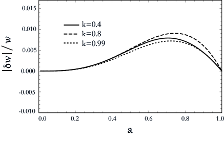
Figure 8: Curves with relative error as a function of scale parameter $a$ for curves (i), (ii) and (iii) of FIG.(7). Note that relative error is at most $\lesssim 0.9\%$.

4.2 Observational viability

Analysis considering Eq. (4.1) for thawing models have already been carried out in Refs.  Dutta2008,Chiba2009c,Chiba2013. For example in Ref. Chiba2009c the likelihood analysis with the SNIa and BAO data was performed. In Ref.  Chiba2013 these analyses were updated by using the Union 2.1 data set [67], the CMB shift parameter measured by WMPA7 [68] and the BAO data of the BOSS experiment [69].

In this subsection we present an updated observational analysis by using the latest SNIa data (JLA sample [66]) and $H(z)$ data [72]. Also, a first attempt to apply Eq. (4.1) to study JpNGB models is developed. Our tests are based on $\chi^{2}$-statistics, which will allow us to explore the space of parameters and constrain the free parameters $\theta$.

Function $\chi^{2}$ is given by

$$\chi^{2}(\theta)=\Delta y^{T}(\theta)\mathbf{C}^{-1}\Delta y(\theta)\,,$$ (24)

where $\Delta y(\theta)=y_{i}-y(x_{i};\theta)$, $\mathbf{C}$ is the covariance matrix of data points $y_{i}$ and $y(x_{i}|\theta)$ represents theoretical predictions for a given set of parameters. The best fit is found by minimizing the $\chi^{2}$-function and the minimum of $\chi^{2}$ gives us an indication of the quality of the fit.

First, we considered tests involving the distance modulus of type Ia Supernovae, which is defined by

$$\mu(z,\theta)=5\,log_{10}(d_{L}(z,\theta))+42.38-5\,log_{10}h\,,$$ (25)

where the luminosity distance is given by

$$d_{L}(z,\theta)=(1+z)H_{0}\int^{z}_{0}\frac{dz^{\prime}}{H(z^{\prime},\theta)}\,.$$ (26)

For our observational treatment with SNIa we used the JLA sample [66] which has 740 data points. This updates a previous analysis performed in [59] based on the Union2.1 data set [67]. Observational data points of the luminosity-distance modulus were calculated using relation [66]

$$\mu_{obs}=m^{*}_{B}-(M_{B}-\alpha X_{1}+\beta C)\,,$$ (27)

where $m^{*}_{B}$ corresponds to the observed peak magnitude in the rest frame $B$ band and $\alpha$, $\beta$ and $M_{B}$ are nuisance parameters, $X_{1}$ is related to the time stretching of the light curves, and $C$ corrects the color at maximum brightness. In order to calculate completely $\mu_{obs}$ and its covariance matrix we have followed the steps suggested in Ref. Betoule2014.

After that, we performed an analysis by using the compilation of observational points for $H(z)$ parameter, which were derived using the differential evolution of passively evolving galaxies as cosmic chronometers [70, 71]. We used the recently updated $H(z)$ data [72] and finally we performed an joint analysis using $\chi^{2}_{total}=\chi^{2}_{SNIa}+\chi^{2}_{H(z)}$.

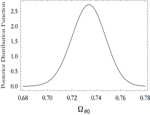
(a)

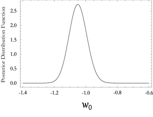
(b)

(c)

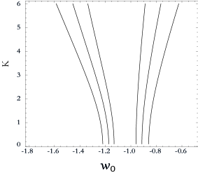
(d)

Figure 9: (a) PDF function for parameter $\Omega_{\phi 0}$ after marginalization on $w_{0}$ and $K$, (b) PDF function for parameter $w_{0}$ after marginalization on $\Omega_{\phi 0}$ and $K$, (c) PDF function of parameter $K$ after marginalization on $\Omega_{\phi 0}$ and $w_{0}$ and (d) $w_{0}$ - $K$ plane with contour lines at 1$\sigma$, 2$\sigma$ and 3$\sigma$ CL.

Considering Eq (4.1) in an observational context of $\mu(z,\theta)$ and $H(z)$ leads us having 4 free parameters ($h$, $\Omega_{\phi 0}$, $w_{0}$ and $K$). However, we have marginalized over parameter $h$ with the prior $50km\,s^{-1}Mpc^{-1}\leq H_{0}\leq 80km\,s^{-1}Mpc^{-1}$ in all of our analyses. Thus, we leave all other three parameters free. As discussed in [59] and for reasons related to approximation limits of Eq. (4.1), we used a prior $0<K<10$. Using SNIa alone, our results give us the constraint of $\Omega_{\phi 0}=0.73^{+0.06}_{-0.07}$, $w_{0}=-1.13^{+0.15}_{-0.17}$ and $K=0.99^{+8}_{-0.99}$ ($2\sigma$ CL). Using $H(z)$ alone our results give us the constraints for $\Omega_{\phi 0}=0.72^{+0.05}_{-0.05}$, $w_{0}=-0.80^{-0.30}_{+0.35}$ and $K=0.1^{+8.5}_{-0.1}$ ($2\sigma$ CL), while the joint analysis gives us $\Omega_{\phi 0}=0.73^{+0.04}_{-0.05}$, $w_{0}=-1.05^{+0.13}_{-0.17}$ and $K=0.99^{+8.2}_{-0.99}$ ($2\sigma$ CL) with a $\chi^{2}_{\nu}\sim 1.1$. Results of the joint analysis are presented in FIG. (9). FIG. 9 (a) shows us the PDF function of the parameter $\Omega_{\phi 0}$ after marginalization over $w_{0}$ and $K$. FIG. 9 (b) shows us the PDF function for parameter $w_{0}$ after marginalization on $\Omega_{\phi 0}$ and $K$. FIG. 9 (c) shows us the PDF function for parameter $K$ after marginalization on $\Omega_{\phi 0}$ and $w_{0}$. Finally FIG. 9 (d) visualizes the $w_{0}$ - $K$ plane with contour lines at 1$\sigma$, 2$\sigma$ and 3$\sigma$ confidence levels. Our results here are in agreement with results in [59]. It can be seen that there is a very high degeneration for parameter $K$.

So far, we have considered the parameter $K$. However, in general, this parameter is not adequate to discriminate between different thawing models through the data. Since we are interested in knowing if JpNGB models are preferred or ruled out by the observations, it is necessary to consider $K$ as a function of parameter $k$. Actually, $K$ is dependent on of $\phi_{i}/f$ also. However, since $\phi_{i}/f$ and $k$ are poorly constrained by data considered here, we will fix the value of $\phi_{i}/f$ and vary the other three parameters. This will allow us to have information about the remaining parameters, particularly of the $k$ parameter.

Thus, considering Eqs. (4.1), (22) and (2) we have performed a new analysis where free parameters are now $\Omega_{\phi 0}$, $w_{0}$ and $k$ where we have fixed $\phi_{i}/f=1.9$. Using SNIa alone our results give us constraints for $\Omega_{\phi 0}=0.76^{+0.06}_{-0.05}$, $w_{0}=-1.16^{-0.14}_{+0.14}$ and $k=0.62^{+0.8}_{-0.62}$ ($2\sigma$ CL). By using $H(z)$ alone our results give us constraints for $\Omega_{\phi 0}=0.72^{+0.05}_{-0.05}$, $w_{0}=-0.83^{-0.30}_{+0.32}$ and $k=0.8^{+0.5}_{-0.8}$ ($2\sigma$ CL), while the joint analyses gives us $\Omega_{\phi 0}=0.73^{+0.04}_{-0.04}$, $w_{0}=-1.06^{+0.11}_{-0.11}$ and $k=0.25^{+0.9}_{-0.25}$ ($2\sigma$ CL) with $\chi^{2}_{\nu}\sim 1.14$. Results of the joint analyses are presented in FIG.(10). FIG. 10 (a) shows us the PDF function for parameter $w_{0}$ after marginalization over $\Omega_{\phi 0}$ and $k$ FIG. 10 (b) shows us the PDF function for parameter $k$ after marginalization over $\Omega_{\phi 0}$ and $w_{0}$ . FIG. 10 (c) shows us the $w_{0}$ - $k$ plane with contour lines at 1$\sigma$, 2$\sigma$ and 3$\sigma$ confidence levels. FIG.10 (d) visualizes the $\Omega_{\phi 0}$ - $w_{0}$ plane with contour lines at 1$\sigma$, 2$\sigma$ and 3$\sigma$ confidence levels. Note that there is a high degeneration in $k$-parameter.

In order to see how our results are affected by $\phi_{i}/f$, we have varied such a parameter in the range $0.6<\phi_{i}/f<2.5$ and we redone the analysis. Results indicate that best-fit values for $\Omega_{\phi_{0}}$ and $w_{0}$ vary in $\sim 5\%$ as maximum. However, best-fit value for $k$ varies $\sim 40\%$. Such high variation is related to the strong degeneration in $k$.

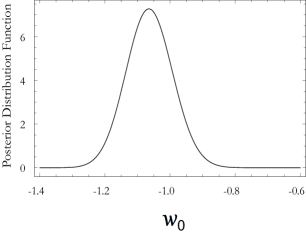
(a)

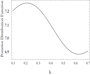
(b)

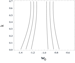
(c)

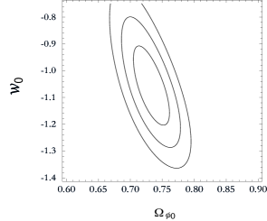
(d)

Figure 10: (a) PDF function for parameter $w_{0}$ after marginalization over $\Omega_{\phi 0}$ and $k$. (b) PDF function for parameter $k$ after marginalization over $\Omega_{\phi 0}$ and $\omega_{0}$. (c) $w_{0}$ -$k$ plane and (d) $\Omega_{\phi 0}$ - $w_{0}$ plane. In (c) and (d) contour lines at 1$\sigma$, 2$\sigma$ and 3$\sigma$ CL are presented.

5 Conclusions

In this work an elliptic generalization of the classical pseudo Nambu–Goldstone potential is studied. We have denominated such a generalization the Jacobian pseudo Nambu–Goldstone (JpNGB) potential. The JpNGB is used as an inflationary potential and we discuss the general conditions of the parameters to describe an inflationary stage. Additionally, we have calculated the values to the inflaton necessary to obtain the number of e–folds of physical expansion required to generate the seeds for the creation of the large structures in the iniverse. Also, the relevant quantities for scalar and tensor perturbations, i.e., the scalar spectral index $n_{s}$ and the scalar–to–tensor ratio $r$, have been calculated explicitly and then contrasted with recent observational data from the Planck collaboration, where marginalized joint $68\%$ and $95\%$ confident level regions for Planck plus WMAP data for the model $\Lambda$CDM plus $r$ were used. These analyses predict that our generalization is able to describe the inflationary stage with exception of potentials with $k\sim 1$.

Afterward, we have used the JpNGB potential and the construction of a family of quintessence models parametrized by parameter $k$ was implemented, where pNGB quintessence is the particular case $k=0$. We solved equations for generalized potential in order to study the evolution of the dynamical EoS and its evolution with the scale factor. It was found that the same initial conditions lead us to a different evolution of EoS for each different $k$, opening the possibility of discriminating between them by using observational data.

As is well known, pGNB is a typical thawing quintessence model. In order to see if similar behavior appears for the family of generalized models, we performed a study of dynamical phase space $w^{\prime}-w$. It was confirmed that such a generalization maintains the thawing features of the pNGB for all the possible values of $k$. This behavior allows us to use an analytical approximation of the dynamical $w(a)$ recently discovered for thawing models.

In order to ascertain whether the generalization is compatible with the observations, we performed an observational analyses using SNIa and $H(z)$ data and the analytical solution for $w(a)$ (Eq. (4.1)). After marginalization over $h$, the space of parameters in this case is $(\Omega_{\phi 0},w_{0},K)$. The best-fit values using SNIa and $H(z)$ joint analyses are $\Omega_{\phi 0}=0.73^{+0.04}_{-0.05}$, $w_{0}=-1.05^{+0.13}_{-0.17}$ and $K=0.99^{+8.2}_{-0.99}$ ($2\sigma$ CL) with a $\chi^{2}_{\nu}\sim 1.1$. These results are in agreement with previous analyses. However, in general, the $K$-parameter is not adequate to discriminate between different thawing models through the data. Since we have been interested in knowing if some generalized model is preferred or ruled out by the observations, it is necessary to consider $K$ as a function of $k$. Thus, after marginalization over $h$ and using a joint analyses with SNIa and $H(z)$, we have as best-fit values $\Omega_{\phi 0}=0.73^{+0.04}_{-0.04}$, $w_{0}=-1.06^{-0.11}_{+0.11}$ and $k=0.25^{+0.9}_{-0.25}$ ($2\sigma$ CL) with a $\chi^{2}_{\nu}\sim 1.14$. These results show us that at 2$\sigma$ CL, JpNGB models with $0\leq k\leq 1$ are not ruled out by SNIa and $H(z)$ data,i.e., quintessence fields with potential (2) with the $\sim 70\%$ of the content of the dark energy and with $w\sim-1$ are compatible with SNIa and $H(z)$ data. Nevertheless it seems to exist a strong degeneration in the $k$-parameter which needs to be broken using another data sets and with a detailed study at perturbative level.

Finally, we can conclude that the generalization considered here is a viable model and it works well overall for the inflationary era and for the acceleration era in late times. Of course a better and a more detailed study is needed that considers the limits of approximation for (4.1) and exact numerical solutions as well as other data sets like CMB or matter power spectrum. Such points are still under investigation.

Appendix A A brief review of Jacobian elliptic functions

The Jacobi elliptic functions are set of elliptic functions whose three basic functions are called the Jacobi elliptic cosine cn $(u,k)$, Jacobi elliptic delta dn $(u,k)$, and Jacobi elliptic sine sn $(u,k)$, where $k$ is known as the elliptic modulus. They arise from the inversion of the elliptic integral of the first kind [74, 76, 75, 73, 77]

$$u(y,k)\equiv u = \int_{0}^{y}\frac{dt}{\sqrt{(1-t^{2})(1-k\,t^{2})}}$$ (28)

$$= \int_{0}^{\varphi}\frac{d\theta}{\sqrt{1-k\sin^{2}\theta}}=F(\varphi,k),$$

which was studied and solved by Abel and Jacobi. The trigonometric and hyperbolic limit are

$$\textrm{sn}(u,0)=\sin u,\quad\textrm{sn}(u,1)=\tanh u,$$ (29)

$$\textrm{cn}(u,0)=\cos u,\quad\textrm{cn}(u,1)=\textrm{sech}\,u,$$ (30)

$$\textrm{dn}(u,0)=1,\,\qquad\,\,\textrm{dn}(u,1)=\textrm{sech}\,u.$$ (31)

The quotients and reciprocal of $\{\textrm{sn}\,u,\,\textrm{cn}\,u,\,\textrm{dn}\,u\}$ are designated in Glaisher’s notation by

$$\textrm{ns}\,u=\frac{1}{\textrm{sn}\,u},\quad\textrm{cs}\,u=\frac{\textrm{cn}\,u}{\textrm{sn}\,u},\quad\textrm{ds}\,u=\frac{\textrm{dn}\,u}{\textrm{sn}\,u},$$ (32)

$$\textrm{nc}\,u=\frac{1}{\textrm{cn}\,u},\quad\textrm{sc}\,u=\frac{\textrm{sn}\,u}{\textrm{cn}\,u},\quad\textrm{dc}\,u=\frac{\textrm{dn}\,u}{\textrm{cn}\,u},$$ (33)

$$\textrm{nd}\,u=\frac{1}{\textrm{dn}\,u},\quad\textrm{sd}\,u=\frac{\textrm{sn}\,u}{\textrm{dn}\,u},\quad\textrm{cd}\,u=\frac{\textrm{cn}\,u}{\textrm{dn}\,u}.$$ (34)

Therefore, in all, we have twelve Jacobian elliptic functions. Finally, some useful fundamental relations between Jacobian elliptic functions are

$$\textrm{sn}^{2}u+\textrm{cn}^{2}u=1,$$ (35)

$$\textrm{dn}^{2}u+k\,\textrm{sn}^{2}u=1,$$ (36)

$$\textrm{dn}^{2}u-k\,\textrm{cn}^{2}u=k^{\prime},$$ (37)

$$\textrm{cn}^{2}u+k^{\prime}\,\textrm{sn}^{2}u=\textrm{dn}^{2}u.$$ (38)

References

- [1] Planck Collaboration (P.A.R. Ade et. al.), Astron. Astrophys. 571 (2014) A16.
- [2] Planck Collaboration (P.A.R. Ade et. al.), arXiv:1502.02114.
- [3] L. Kofman, A. Linde, and A.A. Starobinsky, Phys. Rev. Lett. 73 (1994) 3195.
- [4] L. Kofman, A. Linde, and A.A. Starobinsky, Phys. Rev. D 56 (1997) 3258.
- [5] G. Palma and V.H. Cárdenas, Class. Quant. Grav. 18 (2001) 2233.
- [6] S.E. Joras and V.H. Cárdenas, Phys. Rev. D 67 (2003) 043501.
- [7] A.G. Reiss et al., Astron. J. 116 (1998) 1009.
- [8] S. Perlmutter et al., Astrophys. J. 517 (1999) 565.
- [9] D.N. Spergel et al., Astrophys. J. Suppl. 148 (2003) 175.
- [10] V. Sahni and A. Starobinsky, Int. J. Mod. Phy. D 9 (2000) 373.
- [11] P.J.E. Peebles and B. Ratra, Rev. Mod. Phys. 75 (2003) 559 .
- [12] T.M. Nieuwenhuizen, P.D. Keefe and V. Spicka, J. Cos. 15 6326 (2011).
- [13] L. Amendola et al., Phys. Rev. D 75 (2007) 083504.
- [14] T.P. Sotiriou and V. Faraoni, Rev. Mod. Phys. 82 (2010) 451.
- [15] S. Nojiri and S.D. Odintsov, Phys. Rep. 505 (2011) 59.
- [16] R.F. vom Marttens, W.S. Hipólito-Ricaldi, W. Zimdahl, J. Cosmol. Astropart. Phys. 1408 (2014) 004.
- [17] A. Romero Funo, W.S. Hipólito-Ricaldi, W. Zimdahl, MNRAS 487 (2016) 2958.
- [18] A.Y. Kamenshchik, U. Moschella and V. Pasquier, Phys. Lett. B 511 (2001) 265.
- [19] C. Armendariz–Picon, V.F. Mukhanov and P.J. Steinhardt, Phys. Rev. Lett. 85 (2000) 4438.
- [20] T. Chiba, T. Okabe and M. Yamaguchi, Phys. Rev. D 62 (2000) 023511.
- [21] L.H. Ford, Phys. Rev. D 35 (1987) 2339.
- [22] C. Wetterich, Nucl. Phys. B 302 (1988) 668.
- [23] W.S. Hipólito-Ricaldi, H.E.S. Velten, W. Zimdahl, Phys. Rev. D 82 (2010) 063507.
- [24] E.J. Copeland, M. Sami and S. Tsujikawa, Int. J. Mod. Phys. D 15 (2006) 1753.
- [25] S. Tsujikawa, Class. Quant. Grav. 30 (2013) 214003.
- [26] K. Freese, J.A. Frieman, and A. V. Olinto, Phys. Rev. Lett. 65 (1990) 3233.
- [27] J.A. Frieman, C.T. Hill, A. Stebbins, and I. Waga, Phys. Rev. Lett. 75 (1995) 2077.
- [28] A. Dolgov and K. Freese, Phys. Rev. D 51 (1995) 2693.
- [29] J.A. Espichan-Carillo, J.M.Silva and J.A.S. Lima, arXiv: 0806.3299.
- [30] T.Harko, F.S.N.Lobo, M.K.Mak, Eur. Phys. J. C 74, (2014) 2784.
- [31] A.A. Chaadaev and S.V. Chervon, Russ. Phys. J. 56 , 7, (2013) 725.
- [32] H.-C Kim, Mod. Phys. Lett. A 28, (2013) 1350089.
- [33] P.F. González–Díaz, Phys. Rev. D 62 (2000) 023513.
- [34] T. Higaki and F. Takahashi, J. High Energy Phys. 1503 (2015) 129.
- [35] J.R. Villanueva, J. Cosmol. Astropart. Phys. 07 (2015) 045.
- [36] J.R. Villanueva and E. Gallo, Eur. Phys. J. C 75 (2015) 256.
- [37] T.E. Baker and A. Bill, Am. J. Phys. 80 (2012) 506.
- [38] J.C. Bronski, L.D. Carr, B. Deconinck and N. Kutz, Phys. Rev. Lett. 86 (2001) 1402.
- [39] V.M. Kenkre and M.N. Kuperman, Phys. Rev. E 67 (2003) 051921.
- [40] K. Kajiwara, A. Nobe and T. Tsuda, J. of Physics A 41 (2008) 395202.
- [41] P. Mosconi, G. Mussardo and V. Riva, Nucl. Phys. B 621 (2002) 571.
- [42] B. Bagchi, S. Das and A. Ganguly, Phys. Scr. 82 (2010) 025003.
- [43] A.M. Grundland and S. Post, S J. of Physics A 45 (2012) 015204.
- [44] R.R. Caldwell and E.V. Linder, Phys. Rev. Lett. 95 (2005) 141301.
- [45] C. Kolda and D.H. Lyth, Phys.Lett. B 458 (1999) 197.
- [46] S. M. Carroll, Phys.Rev.Lett. 81, (1998) 3067 .
- [47] T. Chiba, Phys.Rev. D60, (1999) 083508, .
- [48] S. Dutta and R.J. Scherrer, Phys. Rev. D 78 (2008) 123525.
- [49] E.J. Copeland, A.R. Liddle and D. Wands, Phys. Rev. D 57 (1998) 4686.
- [50] R.J. Scherrer and A.A. Sen, Phys. Rev. D 77 (2008) 083515 .
- [51] T.G. Clemson and A.R. Liddle, MNRAS 395 (2009) 1585.
- [52] S.Sen, A.A.Sen and M.Sami, Phys.Lett. B 686 (2010) 1.
- [53] J.García-Bellido, J.Rubio, M.Shaposhnikov and D.Zenhausern, Phys.Rev. D 84 (2011) 123504.
- [54] S. Dutta and R.J.Scherrer, Phys. Lett. B 704 (2011) 265.
- [55] B. Ratra and P.J.E. Peebles, Phys. Rev. D 37 (1988) 3406.
- [56] P.J. Steinhardt, L. Wang, and I. Zlatev, Phys. Rev. D 59 (1999) 123504 .
- [57] P.G. Ferreira and M. Joyce, Phys. Rev. Lett. 79 (1997) 4740.
- [58] T. Chiba, Phys. Rev. D 79 (2009) 083517 .
- [59] T. Chiba, A. De Felice and S. Tsujikawa, Phys. Rev. D 87 (2013) 083505 .
- [60] T. Chiba, Phys. Rev. D 81 (2010) 023515.
- [61] T. Chiba, S. Dutta and R.J. Scherrer, Phys. Rev. D 80 (2009) 043517.
- [62] V. Smer–Barreto and A.R. Liddle, arXiv:1503.06100.
- [63] M. Chevallier, D. Polarski Int. J. Mod. Phys. D10, 213 (2001).
- [64] R. Crittenden, E. Majerotto and F. Piazza, Phys. Rev. Lett. 98 (2007) 25130.
- [65] E. Komatsu et al., Astrophys. J. Suppl. 180 (2009) 330.
- [66] M. Betoule et. al., Astron. Astrophys. 568, (2014) A22.
- [67] N. Suzuki et al., Astrophys. J. 746 (2012) 85 .
- [68] E. Komatsu et al., Astrophys. J. Suppl. 192 (2011) 18.
- [69] L. Anderson et al., Mon. Not. R. Astron. Soc. 427 (2012) 3435.
- [70] J. Simon, L. Verde and R. Jimenez, Phys. Rev. D 71 (2005) 123001.
- [71] D. Stern, R. Jimenez, L. Verde, M. Kamionkowski and S.A. Stanford,
- [72] 0. Farooq and B. Ratra, Astrophys. J. 766 (2013) L7.
- [73] J. Cosmol. Astropart. Phys. 02 (2010) 008 .
- [74] P.F. Byrd and M.D. Friedman, Handbook of elliptic integrals for engineers and scientists, 2nd edn., (Springer–Verlag, Berlin, 1971).
- [75] J.V. Armitage and W.F. Eberlein, Elliptic functions, London Mathematical Society Student Texts (No. 67), (Cambridge University Press, Cambridge, 2006). K. Meyer, Amer. Math. Monthly 108 (2001) 729.
- [76] H. Hancock, Theory of elliptic functions, (Dover publications Inc., New York.,1958).
- [77] I.S. Gradshteyn and I.M. Ryzhik, Table of integrals, series and products, (Academic Press,2007).