Unraveling Quantum Brownian Motion: Pointer States and their Classical Trajectories

Abstract

We characterize the pointer states generated by the master equation of quantum Brownian motion and derive stochastic equations for the dynamics of their trajectories in phase space. Our method is based on a Poissonian unraveling of the master equation whose deterministic part exhibits soliton-like solutions that can be identified with the pointer states. In the semiclassical limit, their phase space trajectories turn into those of classical diffusion, yielding a clear picture of the induced quantum-classical transition.

I Introduction

Decoherence through environmental coupling is a crucial ingredient for understanding the quantum-to-classical transition Joos et al. (2003); Zurek (2003); Schlosshauer (2007). As a prototypical problem, one may consider the motion of a quantum particle interacting with an ideal gas environment. The interaction with the environment selects a preferred set of states, the so-called pointer states Zurek (1981); Zurek et al. (1993); Diósi and Kiefer (2000). These special states of the particle remain pure for a relatively long time, whereas their superpositions decohere very fast into a mixture. For simple master equations the pointer states are known Zurek et al. (1993); Diósi and Kiefer (2000); Eisert (2004); Busse and Hornberger (2009, 2010) to be localized wave packets moving in phase space. In the semiclassical limit they turn into arbitrarily sharp peaks moving along classical phase space trajectories. As such, pointer states are ideally suited to explain the emergence of classicality within a quantum framework.

The name pointer states derives from the fact that their characteristics matches the behavior of a pointer of a measuring apparatus. Namely, if a quantum system is in an eigenstate of the observable we measure with an apparatus its pointer will turn to a specific value on the dial and stay there. On the other hand, if the system is in a superposition of two nondegenerate eigenstates one will not find the pointer of the apparatus to be in a superposition of the two corresponding values, as prescribed by unitarity, but pointing to either one or the other position with probabilities determined by Born’s rule.

In this article, we identify the pointer states of the master equation of quantum Brownian motion (QBM) and derive their equations of motion. Specifically, we understand as QBM the dissipative dynamics of a free particle resulting from many small environmental collisions as described by a Lindblad type master equation Lindblad (1976); Gorini et al. (1976). One possibility to obtain this master equation is to consider a particle linearly coupled to a bath of harmonic oscillators Caldeira and Leggett (1983); Unruh and Zurek (1989); Strunz et al. (2003); Hänggi and Ingold (2005) and to take the high-temperature limit of the reduced particle dynamics; one arrives at the master equation of the Caldeira-Leggett model Caldeira and Leggett (1983); Zurek et al. (1993); Strunz et al. (1999). To get a Lindblad master equation an additional term has to be appended Diósi (1993); Petruccione and Vacchini (2005); Vacchini and Hornberger (2007) making the equation completely positive. Alternatively, the Lindblad master equation of QBM can be obtained by considering a dissipative limit of the general particle motion in a gaseous environment as governed by the so-called quantum linear Boltzmann equation Vacchini (2000); Hornberger (2006); Vacchini and Hornberger (2007, 2009).

By considering quantum trajectories using a particular stochastic process in Hilbert space, the so-called pointer state unraveling, we find the pointer states of QBM to be rotated Gaussians in phase space, in line with the encounter of Gaussian pointer states in other models of linear environmental coupling Eisert (2004); Diósi and Kiefer (2000). Moreover, we show how superpositions of separated wave packets decohere into mixtures of pointer states with weights given by the absolute value of the initial amplitude in the superposition (i.e. Born’s rule). Finally, we derive the stochastic equations of motion for the location of the pointer states in phase space and we show that they turn into the equation of classical diffusion in the semiclassical limit, thus providing a comprehensive picture of the quantum-to-classical transition for the important dissipative process of QBM. For times of evolution much greater than the characteristic decoherence time, it is then justified to approximate the dynamics by a mixture of pointer states moving on trajectories in phase space, instead of calculating the whole evolution of the density matrix.

Our method of using the pointer-state unraveling to identify the pointer basis and to provide a perspective on the quantum-to-classical transition for particle motion has already been demonstrated for the non-dissipative case of pure collisional decoherence Gallis and Fleming (1990); Hornberger and Sipe (2003); Busse and Hornberger (2010). In that case, the pointer states are exponentially localized, rather than Gaussian, and the emerging classical equations of motion are Newton’s equations. In the present case of dissipative dynamics we derive a stochastic equation of motion for the pointer states in order to get the Langevin equation corresponding to classical diffusion. This requires a subtle analysis of the dynamics of the quantum trajectories.

The paper is organized as follows: At first, in section II, we give a general definition of pointer states. In the following section III we introduce and briefly discuss the Lindblad master equation of QBM and introduce its pointer state unraveling. The careful examination of this particular quantum trajectory approach is the topic of the remainder of the paper: The deterministic part of the unraveling is analyzed in section IV providing us with the Gaussian pointer states of QBM as well as with the deterministic part of the classical equations of motion. By looking at the full unraveling, i.e. the deterministic and stochastic part, we show in section V that any superposition of separated wave packets turns into a mixture of pointer states with the expected probabilities. In addition, we identify the trajectories of the pointer states; they exhibit a stochastic motion in phase space and yield diffusion in the semiclassical limit. Section VI contains our conclusions.

II Pointer states

The evolution of a Markovian open quantum system can be described by a Lindblad master equation Gorini et al. (1976); Lindblad (1976); Breuer and Petruccione (2006). For this equation to exhibit pointer states we expect it to display a time scale separation into a short decoherence time $t_{\mathrm{dec}}$ and a much longer dynamical time scale which has also a classical meaning. The set of pointer states is characterized by the property that superpositions of mutually orthogonal pointer states decay into a mixture on the decoherence time scale whereas a single pointer state remains relatively stable and changes on the longer time scale only.

Specifically, for a superposition of pointer states

$$|\psi_{0}\rangle=\sum_{\alpha=1}^{N}c_{\alpha}(0)|\pi_{\alpha}(0)\rangle,$$ (1)

the solution of the master equation for times much greater than $t_{\mathrm{dec}}$ is well approximated by the mixture of pointer states Breuer and Petruccione (2006)

$$\rho_{0}=|\psi_{0}\rangle\langle\psi_{0}|\rightarrow\rho_{t}\simeq\sum_{\alpha=1}^{N}\,\mathrm{Prob(\alpha|\rho_{0})|\pi_{\alpha}(t)\rangle}\langle\pi_{\alpha}(t)|.$$ (2)

A proper set of pointer states forms a basis, is independent of the initial state, and depends only on the environment and the coupling operators. As a consequence and according to Born’s rule, the only dependence of the mixture (2) on the initial state $\rho_{0}$ is via the probabilities

$$\mathrm{Prob}(\alpha|\rho_{0})=\mathrm{Tr}\left(\rho_{0}|\pi_{\alpha}(0)\rangle\langle\pi_{\alpha}(0)|\right)=|c_{\alpha}(0)|^{2}.$$ (3)

The time dependence of the pointer states $|\psi_{\alpha}(t)\rangle$ occurs on the longer time scale only. Once the pointer states and their time dependence are characterized, the dynamics of the master equation is fully captured by Eq. (2) for times greater than $t_{\mathrm{dec}}$.

There are different possibilities to identify the pointer basis. A well-known one requires that the pointer states should be the least entropy producing states of the system; this is the so called predictability sieve Zurek (1993); Dalvit et al. (2005). Here, we follow another approach, in which the pointer states are identified as soliton-like solutions of a nonlinear equation associated with the master equation. This nonlinear pointer state equation (NLPSE) can be obtained heuristically by identifying the pure state evolution closest to the master equation evolution Diósi (1986); Gisin and Rigo (1995).

The pointer state unraveling, a piecewise deterministic stochastic process in Hilbert space, connects the solution of the master equation with the NLPSE, since the latter describes the deterministic part of the unraveling. In the next section, we present the master equation of QBM together with its pointer state unraveling.

III Quantum Brownian motion

III.1 Master equation of quantum Brownian motion

The master equation of QBM describes the quantum state of a massive marker particle linearly coupled to a high-temperature gas environment and experiencing decoherence as well as dissipation. For the sake of simplicity, we restrict ourselves here to the one dimensional case and use dimensionless variables by introducing time, length and momentum scales

$$\mathrm{T}=\frac{1}{2\gamma},\quad\mathrm{L}=\frac{1}{2\gamma}\sqrt{\frac{k_{\mathrm{B}}T_{\mathrm{env}}}{m}},\quad\mathrm{P}=\sqrt{mk_{\mathrm{B}}T_{\mathrm{env}}}.$$ (4)

They involve the mass of the particle $m$, the temperature of the surrounding environment $T_{\mathrm{env}}$, and the friction constant $\gamma$. These scales do not depend on $\hbar$ and are therefore convinient in describing the semiclassical limit of QBM. In these units the canonical commutator takes the form $\left[\hat{\mathsf{x}},\hat{\mathsf{p}}\right]=\mathrm{\mathrm{i}}/\kappa$ and the momentum operator in position representation is $\langle x|\hat{\mathsf{p}}|\Phi\rangle=-\mathrm{\mathrm{i}}/\kappa\,\partial_{x}\Phi(x)$, where we introduced the dimensionless parameter

$$\kappa=\frac{k_{\mathrm{B}}T_{\mathrm{env}}}{2\gamma\hbar}.$$ (5)

The semiclassical limit is then obtained by sending $\kappa\rightarrow\infty$.

The Lindblad master equation of QBM is obtained by using a single Lindblad operator

$$\hat{\mathsf{L}}=\sqrt{2}\left(\kappa\hat{\mathsf{x}}+\frac{\mathrm{\mathrm{i}}}{4}\hat{\mathsf{p}}\right)$$ (6)

and the Hamiltonian

$$\hat{\mathsf{H}}=\hbar\kappa\left(\frac{\hat{\mathsf{p}}^{2}}{2}+\frac{1}{4}\left\{\hat{\mathsf{x}},\hat{\mathsf{p}}\right\}\right).$$ (7)

The anti-commutator $\left\{\hat{\mathsf{x}},\hat{\mathsf{p}}\right\}/4$ describes a rescaling of the particle energy due to the environmental coupling. Inserting (6) and (7) into the general Lindblad master equation Lindblad (1976); Breuer and Petruccione (2006)

$$\frac{\mathrm{d}}{\mathrm{d}t}\rho=\frac{1}{\mathrm{\mathrm{i}}\hbar}\left[\hat{\mathsf{H}},\rho\right]+\left(\hat{\mathsf{L}}\rho\hat{\mathsf{L}}^{\dagger}-\frac{1}{2}\hat{\mathsf{L}}^{\dagger}\hat{\mathsf{L}}\rho-\frac{1}{2}\rho\hat{\mathsf{L}}^{\dagger}\hat{\mathsf{L}}\right),$$ (8)

we arrive at the Lindblad master equation of QBM Vacchini and Hornberger (2007, 2009)

$$\frac{\mathrm{d}}{\mathrm{d}t}\rho =-\mathrm{\mathrm{i}}\frac{\kappa}{2}\left[\hat{\mathsf{p}}^{2},\rho\right]-\mathrm{\mathrm{i}}\frac{\kappa}{2}\left[\hat{\mathsf{x}},\left\{\hat{\mathsf{p}},\rho\right\}\right]-\kappa^{2}\left[\hat{\mathsf{x}},\left[\hat{\mathsf{x}},\rho\right]\right]$$

$$\hskip 10.00002pt-\frac{1}{16}\left[\hat{\mathsf{p}},\left[\hat{\mathsf{p}},\rho\right]\right].$$ (9)

Equation (9) is the Lindblad generalization of the famous Caldeira-Leggett master equation Caldeira and Leggett (1983); Diósi (1993); Breuer and Petruccione (2006), having in common the first three terms on the right-hand side. They describe free motion, friction, and momentum diffusion, respectively. The last term of (9), which ensures complete positivity, can be identified with a position diffusion. This position diffusion term is not present in the Caldeira-Leggett master equation, and its influence decreases with growing $\kappa$.

When writing (9) in the Wigner phase space representation one can draw the semiclassical limit, $\kappa\rightarrow\infty$, to see the formal analogy between the evolution equation for the Wigner function and the Fokker-Planck equation for the classical phase space distribution of classical diffusion Caldeira and Leggett (1983); Vacchini and Hornberger (2007). Further analogies to the classical case of Brownian motion can be seen if one considers the mean values and variances of the position and momentum operators Breuer and Petruccione (2006). Most prominently, one finds that the mean of the momentum operator is exponentially damped and that the variance of the position operator grows linearly for asymptotically large times; both properties are characteristics of classical Brownian motion.

III.2 Unraveling of the master equation

In order to derive the pointer states of QBM and their motion in phase space, we replace the deterministic master equation evolution for the density matrix (9) by an equivalent stochastic pure state evolution in Hilbert space, the pointer state unraveling. The equivalence of an unraveling to a master equation is provided by the fact that the ensemble average over the quantum trajetories yields the solution of the master equation Diósi (1986); Gardiner et al. (1992); Dalibard et al. (1992); Mølmer et al. (1993); Gisin and Rigo (1995); Rigo and Gisin (1996); Busse and Hornberger (2010). Since the decomposition of a density matrix into a mixture of pure states is not unique, many ensembles of quantum trajectories will recover the same solution of the master equation, hence the choice for an unraveling is ambiguous. One distinguishes between continous unravelings based on a Wiener process Gisin (1984); Diosi (1988); Ghirardi et al. (1990); Gisin and Percival (1992); Strunz et al. (1999), where quantum state diffusion is the most prominent, and piecewise deterministic unravelings Diósi (1986); Dalibard et al. (1992); Mølmer et al. (1993); Gisin and Rigo (1995); Busse and Hornberger (2010, 2009) based on a Poisson process.

We will use here a piecewise deterministic unraveling which was already employed in the case of collisional decoherence to determine the pointer states and their dynamics Busse and Hornberger (2010, 2009); Rigo and Gisin (1996). In our case of QBM the deterministic part is formed by the nonlinear operator Gisin and Rigo (1995)

$$\hat{\mathsf{N}}[\psi]|\psi\rangle= \Bigg{(}-\mathrm{\mathrm{i}}\frac{\kappa}{2}\left(\hat{\mathsf{p}}^{2}-\overline{p^{2}}\right)$$

$$\hskip 10.00002pt+\kappa^{2}\left(V_{x}-\left(\hat{\mathsf{x}}-\overline{x}\right)^{2}\right)+\frac{1}{16}\left(V_{p}-\left(\hat{\mathsf{p}}-\overline{p}\right)^{2}\right)$$

$$\hskip 10.00002pt+\frac{\kappa}{4}\left(\mathrm{\mathrm{i}}C_{xp}-\frac{1}{\kappa}\right)-\mathrm{\mathrm{i}}\frac{\kappa}{2}\left(\hat{\mathsf{x}}-\overline{x}\right)\left(\hat{\mathsf{p}}+\overline{p}\right)\Bigg{)}|\psi\rangle,$$ (10)

with expectation values denoted as $\overline{A}=\langle\hat{\mathsf{A}}\rangle=\langle\psi|\hat{\mathsf{A}}|\psi\rangle,$ variances $V_{A}=\overline{A^{2}}-\overline{A}^{2}$ and the covariance $C_{xp}=\overline{\left\{x,p\right\}}-2\overline{x}\,\overline{p}$. Due to the time dependence of the state $|\psi\rangle$, all expectation values are time dependent. The time variable is omitted here for the sake of readability.

The evolution equation

$$\frac{\mathrm{d}}{\mathrm{d}t}|\psi\rangle=\hat{\mathsf{N}}[\psi]|\psi\rangle,$$ (11)

is called the nonlinear pointer state equation (NLPSE) because it is expected to exhibit soliton-like solutions which we will identify as the pointer states. Soliton-like is understood here in the sense that the shape of the wave function is time-independent in phase space. As mentioned above, the NLPSE (11) can also be obtained by looking for the particular pure state equation that mimics the master equation most closely Gisin and Rigo (1995); Diósi and Kiefer (2000).

To obtain the whole unraveling a stochastic jump part must be added to the deterministic NLPSE (11) yielding

$$|\mathrm{d}\psi\rangle =\hat{\mathsf{N}}[\psi]|\psi\rangle\mathrm{d}t+\left(\frac{\hat{\mathsf{J}}[\psi]}{\|\hat{\mathsf{J}}[\psi]|\psi\rangle\|}-1\right)|\psi\rangle\mathrm{d}N,$$ (12)

with the nonlinear jump operator

$$\hat{\mathsf{J}}[\psi] =\sqrt{2}\left(\kappa\left(\hat{\mathsf{x}}-\overline{x}\right)+\frac{\mathrm{\mathrm{i}}}{4}\left(\hat{\mathsf{p}}-\overline{p}\right)\right).$$ (13)

The stochastic Poisson increment $\mathrm{d}N$ can take values $\mathrm{d}N\in\{0,1\}$ and satisfies the Poisson increment rule

$$\mathrm{d}N^{2}=\mathrm{d}N.$$ (14)

The nonlinearity of the jump operator (13) arrises because of its dependence on the position and momentum expectation values which depend on the state $|\psi\rangle$. To fully define the above Poisson process we have to specify the ensemble average of the Poisson increment. It is determined by the rate $r=\langle\psi|\hat{\mathsf{J}}^{\dagger}[\psi]\hat{\mathsf{J}}[\psi]|\psi\rangle$ of the process, given in our case by

$$\frac{\mathrm{E}\left[\mathrm{d}N\right]}{\mathrm{d}t} =r=2\kappa^{2}V_{x}+\frac{1}{8}V_{p}-\frac{1}{2},$$ (15)

with $\mathrm{E}\left[\cdot\right]$ denoting the ensemble average.

A straightforward calculation shows that this unraveling indeed recovers the master equation (9) in the ensemble average Gisin and Rigo (1995). It is also straightforward to verify that the jump rate in this unraveling is proportional to the change of purity of the state

$$r=\frac{1}{2}\frac{\mathrm{d}}{\mathrm{d}t}\mathrm{Tr}\left(1-\left(|\psi\rangle\langle\psi|\right)^{2}\right).$$ (16)

This finding fits with the expected behavior of a pointer state unraveling: Once the pointer state has been reached due to the deterministic part of the unraveling (as determined by the NLPSE) it should be relatively stable. This implies that the change of purity of the pointer state is small and so is therefore the total jump rate (16). As a consequence, once a pointer state is formed in a quantum trajectory of this unraveling, it remains a pointer state as long as possible.

IV Pointer states of quantum Brownian motion

In this section we present the pointer states of QBM as soliton-like solutions of the NLPSE (11). After that we analyze the action of the NLPSE on a superposition of separated wave packets, which will help us to obtain Born’s rule in section V.

IV.1 Single wave packets

A lengthy but straightforward calculation confirms that the NLPSE (11) is solved by a Gaussian state of the form

$$\psi(x) =\frac{1}{\left(2\pi V_{x}\right)^{1/4}}\exp\Bigg{(}-\frac{\left(x-\overline{x}\right)^{2}}{4V_{x}}\left(1-\mathrm{\mathrm{i}}\kappa C_{xp}\right)$$

$$\hskip 10.00002pt+\mathrm{\mathrm{i}}\kappa\left(x-\overline{x}\right)\overline{p}+\mathrm{\mathrm{i}}\phi\Bigg{)},$$ (17)

where $\phi$ is a time dependent global phase. This requires that the first moments and the variances satisfy the following closed set of differential equations,

$$\frac{\mathrm{d}}{\mathrm{d}t}\overline{x} =\overline{p},$$ (18)

$$\frac{\mathrm{d}}{\mathrm{d}t}\overline{p} =-\overline{p},$$ (19)

$$\frac{\mathrm{d}}{\mathrm{d}t}V_{x} =C_{xp}-V_{x}\left(4\kappa^{2}V_{x}-1\right)+\frac{1-\kappa^{2}C_{xp}^{2}}{16\kappa^{2}},$$ (20)

$$\frac{\mathrm{d}}{\mathrm{d}t}C_{xp} =\frac{1+\kappa^{2}C_{xp}^{2}}{16\kappa^{2}}\,\frac{8-C_{xp}}{V_{x}}-4\kappa^{2}C_{xp}V_{x}.$$ (21)

To see this, one inserts the ansatz (17) into the NLPSE (11) and compares coefficients in powers of $x$. A differential equation for $V_{p}$ is readily derived by noting that the variances of the Gaussian state (17) are related via

$$4V_{x}V_{p}=\frac{1}{\kappa^{2}}+C_{xp}^{2}.$$ (22)

The equations of motion (18) and (19) for the first moments exhibit an exponential momentum damping, which reflects the friction experienced by the Brownian particle through the interaction with the gas environment. This movement does not affect the form of the wave packet but only its position in phase space. The equations of motion (20) and (21) for the variances, however, drive the width and orientation of the wave packet in phase space towards the stable fixed values

$$V_{x\mathrm{,ps}} =\frac{1+\sqrt{1+\left(64\kappa^{2}+1\right)\sqrt{16\kappa^{2}+1}}}{8\kappa^{2}\sqrt{16\kappa^{2}+1}},$$ (23)

$$C_{xp\mathrm{,ps}} =\frac{4\kappa-\sqrt{\sqrt{16\kappa^{2}+1}-1}}{\kappa\sqrt{16\kappa^{2}+1}}.$$ (24)

The label “$\mathrm{ps}$” denotes the pointer state, and $V_{p\mathrm{,ps}}$ can be calculated with the help of (22). These fixed values are obtained by solving the nonlinear equations which arise by setting $\mathrm{d}V_{x}/\mathrm{d}t=\mathrm{d}C_{xp}/\mathrm{d}t=0$; their stability can be confirmed by a linear stability analysis of (20) and (21) around $V_{x\mathrm{,ps}}$ and $C_{xp\mathrm{,ps}}$.

A wave packet with the fixed values $V_{x,\mathrm{ps}}$ and $V_{p,\mathrm{ps}}$ is a soliton-like solution in the sense that the form of the wave function in phase space does not change with time. We will call this solution a pointer state of quantum Brownian motion and denote it by $|\pi\left(\overline{x},\overline{p}\right)\rangle$, where $\overline{x}$ and $\overline{p}$ parametrize the position and momentum coordinates of the pointer state. As Gaussian wave functions they form an overcomplete basis set in Hilbert space. From Eqs. (22)-(24) one deduces the asymptotic widths of the pointer states as $\kappa\rightarrow\infty$,

$$V_{x\mathrm{,ps}} \sim\frac{1}{2\kappa^{3/2}},$$ (25)

$$V_{p\mathrm{,ps}} \sim\frac{1}{\kappa^{1/2}},$$

$$C_{xp\mathrm{,ps}} \sim\frac{1}{\kappa}.$$

The pointer states thus get more and more localized in phase space as one goes deeper into the semiclassical regime ($\hbar\rightarrow 0$) characterized by $\kappa\rightarrow\infty$, see Eq. (5). This is illustrated in Fig. 1.

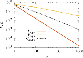
Figure 1: Pointer state variances $V_{x\mathrm{,ps}}$ in position (solid line) and $V_{p\mathrm{,ps}}$ momentum space (dashed line) and covariance $C_{xp,\mathrm{ps}}$ (dotted line) as a function of $\kappa$. For $\kappa\gg 1$, i.e. in the semiclassical limit, all curves follow a potential law. The scales are defined in Eq. (4).

IV.2 Superposition of wave packets

We now analyze the action of the NLPSE (11) on a superposition of separated wave packets. We will see that the NLPSE suppresses such superpositions until only a single localized wave packet remains, which eventually turns into a pointer state $|\pi\left(\overline{x},\overline{p}\right)\rangle$ introduced before.

We consider an initial superposition state of the form

$$|\psi\rangle=\sum_{j}c_{j}(0)|\psi_{j}\rangle,$$ (26)

where the wave packets $|\psi_{j}\rangle$ are well separated in phase space, orthogonal, and normalized with weights

$$w_{j}(0)=\left|c_{j}(0)\right|^{2},$$ (27)

summing up to unity. We drop the time argument of the weights and amplitudes for better readability, and we denote expectation values of the wave packet components as $\overline{A}_{j}=\langle\psi_{j}|\hat{\mathsf{A}}|\psi_{j}\rangle$, and the variances and covariance accordingly.

The $|\psi_{j}\rangle$ are required to be well separated wave packets in the sense that the orthogonality condition

$$\langle\psi_{j}|\hat{\mathsf{A}}|\psi_{k}\rangle=\delta_{jk}\langle\psi_{j}|\hat{\mathsf{A}}|\psi_{j}\rangle\;\forall j,k,$$ (28)

holds for the operators $\text{$\hat{\mathsf{A}}\in$\{$\hat{\mathbb{I}}$},\hat{\mathsf{x}},\hat{\mathsf{x}}^{2},\hat{\mathsf{p}},\hat{\mathsf{p}}^{2},\hat{\mathsf{x}}\hat{\mathsf{p}}+\hat{\mathsf{p}}\hat{\mathsf{x}}\}$. The shape of the $|\psi_{j}\rangle$ can be arbitrary, but their widths in phase space shall be close to that of a pointer state. In particular, we require that the variances $V_{x,j}$ and $V_{p,j}$ of the wave packet components $|\psi_{j}\rangle$ exhibit the same dependence (25) on $\kappa$ as the pointer state. The orthogonality condition (28) can then be fulfilled arbitrarily well by increasing the parameter $\kappa$, which decreases the pointer state width in phase space according to (25), and thus further orthogonalizes the $|\psi_{j}\rangle$.

For the following, it is useful to express the expectation values of the superposition state $|\psi\rangle$ with the help of those of the constituting wave packets $|\psi_{j}\rangle$:

$$\overline{x} =\sum_{j}w_{j}\overline{x}_{j},$$ (29)

$$\overline{p} =\sum_{j}w_{j}\overline{p}_{j},$$

$$V_{x} =\sum_{j}w_{j}V_{x,j}+\frac{1}{2}\sum_{j,k}w_{j}w_{k}\left(\overline{x}_{j}-\overline{x}_{k}\right)^{2},$$

$$V_{p} =\sum_{j}w_{j}V_{p,j}+\frac{1}{2}\sum_{j,k}w_{j}w_{k}\left(\overline{p}_{j}-\overline{p}_{k}\right)^{2},$$

$$C_{xp} =\sum_{j}w_{j}C_{xp,j}+\sum_{j,k}w_{j}w_{k}\left(\overline{x}_{j}-\overline{x}_{k}\right)\left(\overline{p}_{j}-\overline{p}_{k}\right).$$

By inserting the superposition state (26) into the NLPSE (11) we get the expression

$$\frac{\mathrm{d}}{\mathrm{d}t}|\psi\rangle=\sum_{j}\frac{\mathrm{d}}{\mathrm{d}t}\left(c_{j}\right)|\psi_{j}\rangle+c_{j}\frac{\mathrm{d}}{\mathrm{d}t}|\psi_{j}\rangle=\sum_{j}c_{j}\hat{\mathsf{N}}[\psi]|\psi_{j}\rangle,$$ (30)

where the nonlinear operator on the right-hand side contains expectation values with respect to $|\psi\rangle$. From this equation we deduce a set of coupled equations for the normalized states $|\psi_{j}\rangle$ and their weights $w_{j}=|c_{j}|^{2}$:

$$\frac{\mathrm{d}}{\mathrm{d}t}|\psi_{j}\rangle =\hat{\mathsf{N}}[\psi_{j}]|\psi_{j}\rangle+\left(\kappa\left(\hat{\mathsf{x}}-\overline{x}_{j}\right)+\frac{\mathrm{\mathrm{i}}}{4}\left(\hat{\mathsf{p}}-\overline{p}_{j}\right)\right)$$

$$\hskip 10.00002pt\times\left(\kappa\left(\overline{x}-\overline{x}_{j}\right)-\frac{\mathrm{\mathrm{i}}}{4}\left(\overline{p}-\overline{p}_{j}\right)\right)|\psi_{j}\rangle,$$ (31)

$$\frac{\mathrm{d}}{\mathrm{d}t}w_{j} =w_{j}\Bigg{(}2\kappa^{2}\left(V_{x}-V_{x,j}-\left(\overline{x}-\overline{x}_{j}\right)^{2}\right)$$

$$\hskip 10.00002pt+\frac{1}{8}\left(V_{p}-V_{p,j}-\left(\overline{p}-\overline{p}_{j}\right)^{2}\right)\Bigg{)}.$$ (32)

Note, that the nonlinear operator appearing in (31) now only contains expectation values with respect to $|\psi_{j}\rangle.$ Moreover, if there is only one constituent in the “superposition”, Eqs. (31) and (32) turn consistently into the NLPSE (11) and the trivial evolution $\mathrm{d}w_{j}/\mathrm{d}t=0$ for the weight. This is seen most clearly by looking at the differences of the expectation values, which vanish in that case.

The coupled weight equations (32) exhibit a fixed point if a single $w_{j}$ is equal to one, while all others are zero. It can be checked by a linear stability analysis that this fixed point is a stable one. Thus, Eq. (32) expresses the fact that the NLPSE suppresses superpositions of pointer states, since the dynamics of the weights always ends up in the stable fixed point.

To illustrate the suppression of a superposition state, we consider a superposition of two pointer states. The weight of the first component $|\psi_{1}\rangle$ then follows the differential equation

$$\frac{\mathrm{d}}{\mathrm{d}t}w_{1} =\left(2w_{1}-1\right)w_{1}w_{2}\left(2\kappa^{2}\left(\overline{x}_{2}-\overline{x}_{1}\right)^{2}+\frac{1}{8}\left(\overline{p}_{2}-\overline{p}_{1}\right)^{2}\right).$$ (33)

We see immediately that $w_{1}$ gets greater if and only if it is already the greater of the two weights, leading eventually to the suppression of the other component. If there exists a superposition of many wave packets, which, in addition, all have different widths the situation becomes far more complex and can not be captured intuitively. However, the eventual decay of the superposition into one of the components is certain, though it is not easily predictable which component of the superposition will survive in the course of the evolution due to Eq. (32).

V Unraveling quantum Brownian motion

In this section we return to the unraveling of QBM, which consists of the NLPSE as deterministic part, complemented by stochastic jumps. This stochastic part is neccessary to produce the required ensemble of quantum trajetories since the NLPSE alone would always lead to the same asymptotic pointer state for one particular initial state. We first show how the jump process leads to stochastically selected asymptotic pointer states, which occur with relative frequencies according to Born’s rule. After that, in section V.2, we discuss the action of the unraveling on a single pointer state. The NLPSE describes pointer state trajectories which are exponentially damped in momentum. We will see how the stochastic part induces a random walk of the pointer state trajectory displaying the expected diffusive behavior. In the semiclassical limit this will eventually yield classical diffusion.

V.1 Stochastic dynamics of a superposition

Let us consider the action of a single jump on the superposition state (26) of section IV.2, consisting of wave packets $|\psi_{j}\rangle$ that are well separated in phase space, according to the orthogonality relation (28), and with widths comparable to the pointer state width,

$$|\psi^{\prime}\rangle=\frac{\hat{\mathsf{J}}[\psi]|\psi\rangle}{\sqrt{\langle\hat{\mathsf{J}}^{\dagger}\hat{\mathsf{J}}\rangle}}=\sum_{j}c_{j}^{\prime}|\psi_{j}^{\prime}\rangle.$$ (34)

Here, we introduced the normalization factor $\langle\hat{\mathsf{J}}^{\dagger}\hat{\mathsf{J}}\rangle=\langle\psi|\hat{\mathsf{J}}^{\dagger}[\psi]\hat{\mathsf{J}}[\psi]|\psi\rangle$ and the normalized wave packets

$$|\psi_{j}^{\prime}\rangle =\frac{\hat{\mathsf{J}}[\psi]|\psi_{j}\rangle}{\sqrt{\langle\hat{\mathsf{J}}^{\dagger}\hat{\mathsf{J}}\rangle_{j}}},$$ (35)

involving the normalization factor

$$\langle\hat{\mathsf{J}}^{\dagger}\hat{\mathsf{J}}\rangle_{j}=\langle\psi_{j}|\hat{\mathsf{J}}^{\dagger}[\psi]\hat{\mathsf{J}}[\psi]|\psi_{j}\rangle =2\kappa^{2}\left(V_{x,j}+\left(\overline{x}-\overline{x}_{j}\right)^{2}\right)$$

$$\hskip 10.00002pt+\frac{1}{8}\left(V_{p,j}+\left(\overline{p}-\overline{p}_{j}\right)^{2}\right)-\frac{1}{2}.$$ (36)

In the following, only the squared moduli $w_{j}^{\prime}=\left|c_{j}^{\prime}\right|^{2}$ of the new coefficients will be required. One readily finds

$$w_{j}^{\prime}=\left|c_{j}\right|^{2}\frac{\langle\hat{\mathsf{J}}^{\dagger}\hat{\mathsf{J}}\rangle_{j}}{\langle\hat{\mathsf{J}}^{\dagger}\hat{\mathsf{J}}\rangle}.$$ (37)

Note that the new wave packet components $|\psi_{j}^{\prime}\rangle$ can be safely assumed to be still separated and localized because the jump operator modifies the shape only linearly in $\hat{\mathsf{x}}$ and $\hat{\mathsf{p}}$. The superposition state (34) after the jump is therefore again a superposition of separated wave packets, but with different weights. The effect of a jump can thus be approximately accounted for by a reshuffling of a finite number of weights $w_{j}$ in the superposition. We confirmed this by a numerical implementation of the unraveling (12) by combining the Crank-Nicolson method with the split-operator technique Fleck et al. (1976); Feit et al. (1982); Press et al. (2007).

From the action of the NLPSE on a superposition state we calculated in section IV.2 the deterministic evolution (32) of the weights $w_{j}$. Knowing the new weights (37) due to a jump, we are now in a position to construct a stochastic process for the weights of the wave packets where the jumps occur with the same rate as in the original unraveling:

$$\mathrm{d}w_{j} =w_{j}\left(\langle\hat{\mathsf{J}}^{\dagger}\hat{\mathsf{J}}\rangle-\langle\hat{\mathsf{J}}^{\dagger}\hat{\mathsf{J}}\rangle_{j}\right)\mathrm{d}t$$

$$\hskip 10.00002pt+w_{j}\left(\frac{\langle\hat{\mathsf{J}}^{\dagger}\hat{\mathsf{J}}\rangle_{j}}{\langle\hat{\mathsf{J}}^{\dagger}\hat{\mathsf{J}}\rangle}-1\right)\mathrm{d}N.$$ (38)

Here, we have written the deterministic part (32) more conveniently with the help of the jump rate $r=\langle\hat{\mathsf{J}}^{\dagger}\hat{\mathsf{J}}\rangle$ (15) and the normalization factor $\langle\hat{\mathsf{J}}^{\dagger}\hat{\mathsf{J}}\rangle_{j}$ (36). The Poisson increment $\mathrm{d}N$ has the same ensemble average $\mathrm{E}[\mathrm{d}N]=r\,\mathrm{d}t$ as the pointer state unraveling (12).

The set of equations (38) represent the evolution of the weights in a quantum trajectory. Each quantum trajectory ends up asymptotically in a pointer state, when all weights but a single one vanish. From this we deduce that the relative frequency of finding a particular pointer state $|\pi\left(\overline{x}_{j},\overline{p}_{j}\right)\rangle$ is equal to the probability of the associated asymptotic state in the ensemble of quantum trajectories. This latter probability is evaluated easily by carrying out the ensemble average of (38),

$$\mathrm{E}\left[\mathrm{d}w_{j}\right] =0.$$ (39)

This implies $\mathrm{E}\left[w_{j}(t)\right]=\mathrm{const}.$ and, in particular,

$$\mathrm{E}\left[w_{j}(t\rightarrow\infty)\right]=\mathrm{E}\left[w_{j}(0)\right]=|c_{j}(0)|^{2},$$ (40)

where $c_{j}(0)$ are the initial amplitudes of the wave packets in the superposition state (26). Equation (40) confirms Born’s rule (3), as expected for a superposition of separated wave packets.

V.2 Stochastic dynamics of a single wave packet

So far, we investigated the dynamics of the unraveling if the initial state is a superposition of localized wave packets. We confirmed in the previous section that the probability to end up asymptotically in a certain pointer state is given by its weight in the initial superposition (Born’s rule). This process takes place on the fast decoherence time scale $t_{\mathrm{dec}}$ after which the system is well described by a pointer state. In terms of the pointer state unraveling, this point is reached when each quantum trajectory in the ensemble has turned into its asymptotic pointer state.

Since the underlying quantum dynamics is diffusive Breuer and Petruccione (2006) it is natural to describe the statistics of the position $\overline{x}$ and the momentum $\overline{p}$ of the pointer state by the phase space diffusion

$$\left(\begin{aligned} \mathrm{d}\overline{x}\\ \mathrm{d}\overline{p}\end{aligned}\right)=\left(\begin{aligned} \overline{p}\\ -\overline{p}\end{aligned}\right)\mathrm{d}t+\left(\begin{array}[]{cc}B_{11}&B_{12}\\ B_{21}&B_{22}\end{array}\right)\left(\begin{array}[]{c}\mathrm{d}W_{1}\\ \mathrm{d}W_{2}\end{array}\right),$$ (41)

with the Wiener increments $\mathrm{d}W_{1}$ and $\mathrm{d}W_{2}$ obeying the rules

$$\mathrm{E}[\mathrm{d}W_{i}] =0,$$ (42)

$$\mathrm{d}W_{i}\mathrm{d}W_{j} =\delta_{ij}\mathrm{d}t.$$

Equation (41) is a special case of the two-dimensional Ornstein-Uhlenbeck process with constant coefficients Gardiner (2009) and the derivation of its ensemble variances and covariance is presented in the appendix. The different diffusion constants $D_{x}$, $D_{p}$, and $D_{xp}$ describing position, momentum, and covariance diffusion are related to the $B_{ij}$ by

$$D_{x} =B_{11}^{2}+B_{12}^{2},$$ (43)

$$D_{p} =B_{21}^{2}+B_{22}^{2},$$

$$D_{xp} =B_{11}B_{21}+B_{12}B_{22}.$$

We proceed to show how the stochastic jumps acting on the motion of the pointer state lead to phase space trajectories which turn into classical diffusion in the semiclassical limit $\kappa\rightarrow\infty$. To achieve this, we derive a simple model allowing the description of the pointer state trajectories by the phase space diffusion (41) and then compare it to a numerical study.

V.2.1 Analytic model

Consider a pointer state moving on the phase space trajectory governed by the NLPSE (see Sec. IV.1). This deterministic motion is interrupted by a jump, described by the jump operator (13) acting on the pointer state (17),

$$\psi^{\prime}(x) =\langle x|\hat{\mathsf{J}}[\pi\left(\overline{x},\overline{p}\right)]|\pi\left(\overline{x},\overline{p}\right)\rangle$$

$$=\sqrt{\frac{2}{r_{\mathrm{ps}}}}\left[\kappa\left(1-\frac{1-\mathrm{\mathrm{i}}\kappa C_{xp\mathrm{,ps}}}{8\kappa^{2}V_{x\mathrm{,ps}}}\right)\left(x-\overline{x}\right)\right]\langle x|\pi\left(\overline{x},\overline{p}\right)\rangle.$$ (44)

Here,

$$r_{\mathrm{ps}}=2\kappa^{2}V_{x,\mathrm{ps}}+\frac{1}{8}V_{p,\mathrm{ps}}-\frac{1}{2}$$ (45)

is the jump rate (15) of the pointer state and $V_{x,\mathrm{ps}}$ and $V_{p,\mathrm{ps}}$ are the widths of the pointer states defined in Eqs. (22)-(24). The resulting state is a symmetric double-peaked wave packet. This symmetry reflects the assumed symmetry of the state before the jump. Since in reality the system state is never exactly symmetric even small asymmetries will trigger the emergence of a single wave packet under the NLPSE, see Fig. 2.

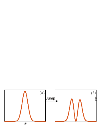
Figure 2: Simplified jump process: A jump turns the wave packet at position $\overline{x}$ $(a)$ into a slightly asymmetric double-peaked structure $(b)$. The NLPSE then suppresses one of the peaks resulting in a single wave packet at the position $\overline{x}^{\prime}$ of one of the double-peaks $(c)$. A similar picture applies in momentum space.

Which of the two subpeaks survives depends on the asymmetry before the jump. We assume equal probabilities and that the single wave packet is restored sufficiently fast by the NLPSE. This results in an effective jump of the pointer state’s first moments in phase space by the distances

$$j_{x} =|\overline{x}^{\prime}-\overline{x}|=\sqrt{2V_{x\mathrm{,ps}}},$$ (46)

$$j_{p} =|\overline{p}^{\prime}-\overline{p}|=\sqrt{2V_{p\mathrm{,ps}}}.$$

The widths $j_{x}$ and $j_{p}$ are calculated from the positions of the two peaks in (44). Since the direction of the jump is positive or negative with equal probability, we end up with the two possible jumps in phase space

$$\vec{j}_{1} =\left(\begin{array}[]{c}j_{x}\\ j_{p}\end{array}\right), \vec{j}_{2} =\left(\begin{array}[]{c}-j_{x}\\ -j_{p}\end{array}\right),$$ (47)

each of them characterized by a Poisson process $\mathrm{d}N_{k}$ with jump rate

$$r_{k} =\frac{\mathrm{E}[\mathrm{d}N_{k}]}{\mathrm{d}t}=\frac{r_{\mathrm{ps}}}{2}.$$ (48)

We are now in the position to write down a stochastic differential equation for $\overline{x}$ and $\overline{p}$,

$$\left(\begin{aligned} \mathrm{d}\overline{x}\\ \mathrm{d}\overline{p}\end{aligned}\right) =\left(\begin{aligned} \overline{p}\\ -\overline{p}\end{aligned}\right)\mathrm{d}t+\sum_{k=1}^{2}\vec{j}_{k}\mathrm{d}N_{k}.$$ (49)

It consists of the deterministic evolution (18) and (19) derived in section IV.1 and the stochastic jumps (47) with corresponding jump rates (48). By using the Poisson rule $\mathrm{d}N_{k}\mathrm{d}N_{l}=\delta_{kl}\mathrm{d}N_{k}$ and Eq. (48), one can easily derive all moments of the stochastic process (49),

$$\mathrm{E}\left[\left(\mathrm{d}x\right)^{2n-1}\right]=0, \mathrm{E}\left[\left(\mathrm{d}x\right)^{2n}\right]=j_{x}^{2n}r_{\mathrm{ps}}\mathrm{d}t,$$

$$\mathrm{E}\left[\left(\mathrm{d}p\right)^{2n-1}\right]=0, \mathrm{E}\left[\left(\mathrm{d}p\right)^{2n}\right]=j_{p}^{2n}r_{\mathrm{ps}}\mathrm{d}t,$$ (50)

$$\mathrm{E}\left[\left(\mathrm{d}x\mathrm{d}p\right)^{n}\right]=\left(j_{x}j_{p}\right)^{n}r_{\mathrm{ps}}\mathrm{d}t,$$

with $n\geq 1$. If one is interested in calculating moments up to second order only, the stochastic jump process (49) can be well approximated by the phase space diffusion (41) upon identifying the diffusion constants (43) with

$$D_{x} =j_{x}^{2}r_{\mathrm{ps}},$$

$$D_{p} =j_{p}^{2}r_{\mathrm{ps}},$$ (51)

$$D_{xp} =j_{x}j_{p}r_{\mathrm{ps}}.$$

Inserting the jump widths (46) and the jump rate (45) into Eqs. (51) one gets their dependence on $\kappa$ as $\kappa\rightarrow\infty$

$$D_{x} \sim\frac{1}{\kappa},$$ (52)

$$D_{p} \sim 2,$$

$$D_{xp} \sim\frac{1}{\kappa^{1/2}}.$$

We see that both $D_{x}$ and $D_{xp}$ vanish in the semiclassical limit $\kappa\rightarrow\infty$ so that only the momentum diffusion $D_{p}=2$ contributes and the stochastic process (41) thus reduces to

$$\left(\begin{aligned} \mathrm{d}\overline{x}\\ \mathrm{d}\overline{p}\end{aligned}\right) =\left(\begin{aligned} \overline{p}\\ -\overline{p}\end{aligned}\right)\mathrm{d}t+\left(\begin{aligned} 0\\ \sqrt{D_{p}}\end{aligned}\right)\mathrm{d}W.$$ (53)

One can also arrive directly at (53) without defining the phase space diffusion (41) by drawing the semiclassical limit of Eq. (49) and thereby performing a diffusive limit analogous to that of a random walker Gardiner (2009). Writing (53) in physical dimensions by using the scales defined in Eq. (4) finally leads to the Langevin equation of classical Brownian motion Risken (1989); Breuer and Petruccione (2006)

$$\mathrm{d}\overline{p}=-2\gamma\overline{p}\mathrm{d}t+\sqrt{4\gamma mk_{\mathrm{B}}T_{\mathrm{env}}}\mathrm{d}W,$$ (54)

where the dimension of $\mathrm{d}W$ is a square root of time.

It should be remarked here, that the crucial assumption leading to this model is the immediate restoring of the pointer state after a jump. The real dynamics will take a finite time until the double-peaked wave function returns to a pointer state, and there will be several jumps in between. We show in the following, by numerically simulating trajectories of the pointer state unraveling, that this is indeed the case, giving rise to complex dynamics. Nonetheless, the general picture of the analytic model can be confirmed.

V.2.2 Numerical study

Using a combination of the Crank-Nicolson method and a split-operator technique Fleck et al. (1976); Feit et al. (1982); Press et al. (2007) we generated quantum trajectories of the unraveling (12) and calculated their first moments $\overline{x}$ and $\overline{p}$ and their variances $V_{x}$, $V_{p}$ and $C_{xp}$.

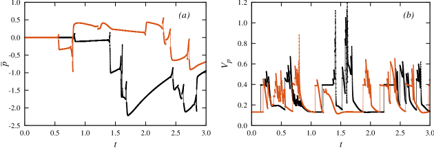
Figure 3: $(a)$ momentum expectation $\overline{p}$ and $(b)$ momentum variance $V_{p}$ of two sample trajectories starting at the same pointer state $|\pi\left(0,0\right)\rangle$. One observes that in general more than a single jump occurs in the unraveling before the width of the wave function is restored to the pointer state width. The calculations are made at $\kappa=50$ and all quantities are dimensionless with scales defined in Eq. (4).

Figure 3 shows exemplarily the temporal evolution of $\overline{p}$ and $V_{p}$ for two sample trajectories. A similar behavior is found in position space (not shown).

Verification of the stochastic model

In order to compare the statistics of the phase space trajectories predicted by the phase space diffusion (41) with that of the numerically generated trajectories we consider the expectation values of a finite sample of size $N$

$$\mathrm{E}_{N}[x] =\frac{1}{N}\sum_{i=1}^{N}\overline{x}_{i},$$

$$\mathrm{E}_{N}[p] =\frac{1}{N}\sum_{i=1}^{N}\overline{p}_{i},$$

$$\mathrm{Var}_{N}[x] =\frac{1}{N-1}\sum_{i=1}^{N}\left(\overline{x}_{i}-\mathrm{E}_{N}[x]\right)^{2},$$ (55)

$$\mathrm{Var}_{N}[p] =\frac{1}{N-1}\sum_{i=1}^{N}\left(\overline{p}_{i}-\mathrm{E}_{N}[p]\right)^{2},$$

$$\mathrm{Cov}_{N}[x,p] =\frac{1}{N-1}\sum_{i=1}^{N}\left(\overline{x}_{i}-\mathrm{E}_{N}[x]\right)\left(\overline{p}_{i}-\mathrm{E}_{N}[p]\right),$$

where $\overline{x}_{i}$, $\overline{p}_{i}$ are the first moments of quantum trajectory $i$. The sample expectation values (55) are themselves stochastic values due to the stochasticity of the underlying model. The ensemble variances of $\mathrm{E}_{N}\left[x\right]$ and $\mathrm{E}_{N}\left[p\right]$ on the one hand and those of $\mathrm{Var}_{N}[x]$, $\mathrm{Var}_{N}[p]$, and $\mathrm{Cov}_{N}[x,p]$ on the other are proportional to $1/N$ and $1/\left(N-1\right)$, respectively (see appendix). We compare the finite-size variances of the numerically generated trajectories with those predicted by the above model.

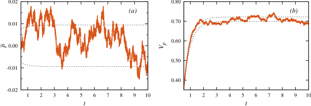
Figure 4: $\mathrm{E}_{N}\left[p\right]$ and $\mathrm{Var}_{N}\left[p\right]$ (solid) as well as their theoretically expected deviations (dashed) due to a finite sample size. The fluctuations are well characterized by the dashed lines. Calculations are done at $\kappa=50$ for $N=8000$ trajectories.

Figure 4 compares $\mathrm{E}_{N}\left[p\right]$ and $\mathrm{Var}_{N}\left[p\right]$ of the sample with the theoretically expected deviations. The interval of one standard deviation around the ensemble mean value $\mathrm{E}_{\infty}\left[p\right]$ should contain $\approx 68\%$ of the trajectories of the sample, which we confirmed at selected times. The same analysis applies for $\mathrm{E}_{N}[x]$, $\mathrm{Var}_{N}[x]$, and $\mathrm{Cov}_{N}[x,p]$ and yields the same result. Thus, we conclude that the statistics of the moments of the pointer state unraveling can indeed be described by the stochastic model (41).

Extraction of the diffusion constants

Having verified the stochastic model we are now able to extract the diffusion constants $D_{x}$, $D_{p}$ and $D_{xp}$ by fitting the variances shown in Eqs. (60) to the generated trajectories. Since $\mathrm{Var}[p]$ only depends on $D_{p}$, and $\mathrm{Cov}[x,p]$ only on $D_{p}$ and $D_{xp}$, fitting is done consecutively by extracting $D_{p}$ from $\mathrm{Var}[p]$, $D_{xp}$ from $\mathrm{Cov}[x,p]$, and finally $D_{x}$ from $\mathrm{Var}[x]$. The numerically obtained values for different $\kappa$, as well as the calculations from the analytic model (52), are shown in Fig. 5.

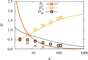
Figure 5: Dependence of the diffusion constants $D_{x}$ (solid line), $D_{p}$ (dashed line) and $D_{xp}$ (dotted line) on $\kappa$. The lines are calculated from Eqs. (51) of the analytic model, whereas the symbols represent the results of the numerical simulation. One observes for all three diffusion constants that the analytic model captures the main features of their dependence on $\kappa$. Specifically, $D_{p}$ approaches the classical value of 2 in the semiclassical regime $\kappa\rightarrow\infty$, whereas $D_{x}$ and $D_{xp}$ vanish in that limit.

We see that the calculated $D_{p}$ is in good quantitative agreement with the simulation. The deviation of the calculated $D_{x}$ and $D_{xp}$ from the simulated ones is due to the crude simplification made by the assumption that a jump in the unraveling corresponds to a phase-space jump of the pointer state without further dynamics; Fig. 3 shows clearly that this is not the case.

For large $\kappa$ both the analytic model and the numerical simulation exhibit the classically expected behavior. Specifically, the position diffusion $D_{x}$ and the covariance diffusion $D_{xp}$ tend to zero, whereas the momentum diffusion $D_{p}$ approaches the value 2.

VI Conclusion

We identified the pointer states of quantum Brownian motion and derived the stochastic equations of motion for their trajectories in phase space. The pointer states turn out to be Gaussian wave packets with fixed widths and a finite position-momentum covariance. The phase space trajectory characterizing their motion obeys a stochastic differential equation combining momentum damping with position and momentum diffusion. In the semiclassical limit, it turns into the Langevin equation of classical diffusion. This provides us with a consistent and transparent picture of the quantum-classical transition as induced by quantum Brownian motion.

We saw that any initial state, which can be represented by a superposition of sufficiently separated wave packets decays into a mixture of corresponding pointer states, and that the ensuing statistical weights are consistent with Born’s rule. Using the pointer states and their trajectories one can thus capture an essential part of the dynamics of quantum Brownian motion. Our analysis depends crucially on linking the nonlinear equation of motion for the pointer states to a particular piecewise deterministic unraveling of the master equation. It allows one to connect the open quantum dynamics to stochastic trajectories in phase space.

The described technique of unraveling a master equation into pointer state trajectories may become particularly useful in cases where even approximate solutions of a master equation are not known. For example, the full Markovian dynamics of a tracer particle in a gaseous environment is described by a complicated integro-differential equation not readily accessible by analytic means Vacchini and Hornberger (2009). If pointer states can be identified for this equation we expect their trajectories to be described by a general Chapman-Kolmogorov equation in phase space turning into the linear Boltzmann equation in the semiclassical limit.

This work was supported by the DFG via SFB/TR 12.

Appendix A Diffusion in phase space

We analyze the properties of the classical stochastic process

$$\mathrm{d}x =p\,\mathrm{d}t+B_{11}\mathrm{d}W_{1}+B_{12}\mathrm{d}W_{2},$$ (56)

$$\mathrm{d}p =-p\,\mathrm{d}t+B_{21}\mathrm{d}W_{1}+B_{22}\mathrm{d}W_{2},$$

used in section V.2 to describe the dynamics of the first moments $\overline{x}$, $\overline{p}$ of the pointer states in phase space. At first, we discuss the ensemble statistics, and afterwards the statistics of a sample of finite size.

A.1 Ensemble statistics

In order to derive the statistical properties of the stochastic process (56), we recall the stochastic properties of the real-valued Wiener increments $\mathrm{d}W_{1}$ and $\mathrm{d}W_{2}$

$$\mathrm{E}[\mathrm{d}W_{i}] =0,$$ (57)

$$\mathrm{d}W_{i}\mathrm{d}W_{j} =\delta_{ij}\mathrm{d}t.$$

From these two relations one can derive a differential equation for e.g. $x^{2}$ by expanding to second order in $\mathrm{d}x$ and keeping only terms to the order $\mathrm{d}t$, known as the Ito rule of stochastic calculus. One gets

$$\mathrm{d}\left(x^{2}\right) =2x\mathrm{d}x+\left(\mathrm{d}x\right)^{2}$$ (58)

$$=\left(2xp+B_{11}^{2}+B_{12}^{2}\right)\mathrm{d}t+2x\left(B_{11}\mathrm{d}W_{1}+B_{12}\mathrm{d}W_{2}\right).$$

In the same manner one calculates $\mathrm{d}\left(p^{2}\right)$ and $\mathrm{d}\left(xp\right)$, which then allows the derivation of differential equations for the ensemble variances $\mathrm{Var}[x]=\mathrm{E}[x^{2}]-\mathrm{E}[x]^{2}$ and $\mathrm{Var}[p]=\mathrm{E}[p^{2}]-\mathrm{E}[p]^{2}$ and the ensemble covariance $\mathrm{Cov}[x,p]=\mathrm{E}[xp]-\mathrm{E}[x]\mathrm{E}[p]$:

$$\frac{\mathrm{d}}{\mathrm{d}t}\mathrm{Var}[x] =2\mathrm{Cov}[x,p]+D_{x},$$ (59)

$$\frac{\mathrm{d}}{\mathrm{d}t}\mathrm{Var}[p] =-2\mathrm{Var}[p]+D_{p},$$

$$\frac{\mathrm{d}}{\mathrm{d}t}\mathrm{Cov}[x,p] =-\mathrm{Cov}[x,p]+\mathrm{Var}[p]+D_{xp},$$

where definition (43) of the diffusion constants was used. Solving the differential equations (59) for initial conditions $\mathrm{Var}[x](0)=\mathrm{Var}[p](0)=\mathrm{Cov}[x,p](0)=0$ yields

$$\mathrm{Var}[x](t) =\left(D_{x}+D_{p}+2D_{xp}\right)t-\frac{1}{2}D_{p}\left(1-\mathrm{e}^{-t}\right)^{2}$$ (60)

$$\hskip 10.00002pt-\left(D_{p}+2D_{xp}\right)\left(1-\mathrm{e}^{-t}\right),$$

$$\mathrm{Var}[p](t) =\frac{1}{2}D_{p}\left(1-\mathrm{e}^{-2t}\right),$$

$$\mathrm{Cov}[x,p](t) =\frac{1}{2}D_{p}\left(1-\mathrm{e}^{-t}\right)^{2}+D_{xp}\left(1-\mathrm{e}^{-t}\right).$$

A.2 Statistics with finite sample size

We are now interested in the statistics of the first moments and the variances of a finite sample of size $N$, and, in particular, their deviations around the ensemble values (60). With the help of the stochastic model (56) and the sample expectation values (55) one can write down e.g. the stochastic differential equation for the sample momentum expectation

$$\mathrm{d}\mathrm{E}_{N}[p] =-\mathrm{E}_{N}[p]\mathrm{d}t+\frac{1}{N}\sum_{i=1}^{N}\left(B_{21}\mathrm{d}W_{1,i}+B_{22}\mathrm{d}W_{2,i}\right),$$ (61)

with independent Wiener increments $\mathrm{d}W_{1,i}$ and $\mathrm{d}W_{2,i}$ for all $i$. In the same manner as in the previous section one can then derive

$$\mathrm{d}\left(\mathrm{E}_{N}[p]^{2}\right) =2\mathrm{E}_{N}[p]\mathrm{d}\mathrm{E}_{N}[p]+\left(\mathrm{d}\mathrm{E}_{N}[p]\right)^{2}$$ (62)

$$=\left(-2\mathrm{E}_{N}[p]^{2}+\frac{B_{21}^{2}+B_{22}^{2}}{N}\right)\mathrm{d}t$$

$$\hskip 10.00002pt+\frac{2}{N}\mathrm{E}_{N}[p]\sum_{i=1}^{N}\left(B_{21}\mathrm{d}W_{1,i}+B_{22}\mathrm{d}W_{2,i}\right),$$

and finally

$$\frac{\mathrm{d}}{\mathrm{d}t}\mathrm{Var}[\mathrm{E}_{N}[p]] =-2\mathrm{Var}[\mathrm{E}_{N}[p]]+\frac{D_{p}}{N}.$$ (63)

Here, the ensemble variance of $\mathrm{E}_{N}\left[p\right]$ is denoted by $\mathrm{Var}[\mathrm{E}_{N}[p]]=\mathrm{E}[\mathrm{E}_{N}[p]^{2}]-\mathrm{E}[\mathrm{E}_{N}[p]]^{2}$ and the definition of the diffusion constants (43) was used.

Similarly, one derives a stochastic differential equation for the sample variance of the momentum

$$\mathrm{d}\mathrm{Var}_{N}[p] =\left(D_{p}-2\mathrm{Var}_{N}[p]\right)\mathrm{d}t+\frac{2}{N-1}\sum_{i=1}^{N}\left(p_{i}-\mathrm{E}_{N}[p]\right)$$

$$\hskip 10.00002pt\times\left(B_{21}\mathrm{d}W_{1,i}+B_{22}\mathrm{d}W_{2,i}\right),$$ (64)

yielding

$$\frac{\mathrm{d}}{\mathrm{d}t}\mathrm{Var}[\mathrm{Var}_{N}[p]] =-4\mathrm{Var}[\mathrm{Var}_{N}[p]]+\frac{4D_{p}\mathrm{Var}[p]}{N-1}$$ (65)

for the ensemble variance of $\mathrm{Var}_{N}[p]$. The variances of $\mathrm{E}_{N}[x]$, $\mathrm{Var}_{N}[x]$ and $\mathrm{Cov}_{N}[x,p]$ are obtained accordingly in a long and tedious calculation, giving the solutions

$$\mathrm{Var}[\mathrm{E}_{N}[x]] =\frac{1}{N}\mathrm{Var}[x],$$ (66)

$$\mathrm{Var}[\mathrm{E}_{N}[p]] =\frac{1}{N}\mathrm{Var}[p],$$

$$\mathrm{Var}[\mathrm{Var}_{N}[x]] =\frac{2}{N-1}\mathrm{Var}[x]^{2},$$

$$\mathrm{Var}[\mathrm{Var}_{N}[p]] =\frac{2}{N-1}\mathrm{Var}[p]^{2},$$

$$\mathrm{Var}[\mathrm{Cov}_{N}[x,p]] =\frac{1}{N-1}\left(\mathrm{Var}[x]\mathrm{Var}[p]+\mathrm{Cov}[x,p]^{2}\right).$$

References

- Joos et al. (2003) E. Joos, H. D. Zeh, C. Kiefer, D. Giulini, J. Kupsch, and I. O. Stamatescu, Decoherence and the Appearance of a Classical World in Quantum Theory (Springer-Verlag Berlin, 2003).
- Zurek (2003) W. H. Zurek, Rev. Mod. Phys. 75, 715 (2003).
- Schlosshauer (2007) M. Schlosshauer, Decoherence and the quantum to classical transition (Springer-Verlag Berlin, 2007).
- Zurek (1981) W. H. Zurek, Phys. Rev. D 24, 1516 (1981).
- Zurek et al. (1993) W. H. Zurek, S. Habib, and J. P. Paz, Phys. Rev. Lett. 70, 1187 (1993).
- Diósi and Kiefer (2000) L. Diósi and C. Kiefer, Phys. Rev. Lett. 85, 3552 (2000).
- Eisert (2004) J. Eisert, Phys. Rev. Lett. 92, 210401 (2004).
- Busse and Hornberger (2009) M. Busse and K. Hornberger, J. Phys. A 42, 362001 (2009).
- Busse and Hornberger (2010) M. Busse and K. Hornberger, J. Phys. A 43, 015303 (2010).
- Lindblad (1976) G. Lindblad, Comm. Math. Phys. 48, 119 (1976).
- Gorini et al. (1976) V. Gorini, A. Kossakowski, and E. C. G. Sudarshan, J. Math. Phys. 17, 821 (1976).
- Caldeira and Leggett (1983) A. Caldeira and A. Leggett, Physica A 121, 587 (1983).
- Unruh and Zurek (1989) W. G. Unruh and W. H. Zurek, Phys. Rev. D 40, 1071 (1989).
- Strunz et al. (2003) W. T. Strunz, F. Haake, and D. Braun, Phys. Rev. A 67, 022101 (2003).
- Hänggi and Ingold (2005) P. Hänggi and G.-L. Ingold, Chaos 15, 026105 (2005).
- Strunz et al. (1999) W. T. Strunz, L. Diósi, N. Gisin, and T. Yu, Phys. Rev. Lett. 83, 4909 (1999).
- Diósi (1993) L. Diósi, Europhys. Lett. 22, 1 (1993).
- Petruccione and Vacchini (2005) F. Petruccione and B. Vacchini, Phys. Rev. E 71, 046134 (2005).
- Vacchini and Hornberger (2007) B. Vacchini and K. Hornberger, Eur. Phys. J. Spec. Top. 151, 59 (2007).
- Vacchini (2000) B. Vacchini, Phys. Rev. Lett. 84, 1374 (2000).
- Hornberger (2006) K. Hornberger, Phys. Rev. Lett. 97, 060601 (2006).
- Vacchini and Hornberger (2009) B. Vacchini and K. Hornberger, Phys. Rep. 478, 71 (2009).
- Gallis and Fleming (1990) M. R. Gallis and G. N. Fleming, Phys. Rev. A 42, 38 (1990).
- Hornberger and Sipe (2003) K. Hornberger and J. E. Sipe, Phys. Rev. A 68, 012105 (2003).
- Breuer and Petruccione (2006) H.-P. Breuer and F. Petruccione, The Theory of Open Quantum Systems (Oxford University Press, 2006).
- Zurek (1993) W. H. Zurek, Prog. Theor. Phys. 89, 281 (1993).
- Dalvit et al. (2005) D. A. R. Dalvit, J. Dziarmaga, and W. H. Zurek, Phys. Rev. A 72, 062101 (2005).
- Diósi (1986) L. Diósi, Phys. Lett. A 114, 451 (1986).
- Gisin and Rigo (1995) N. Gisin and M. Rigo, J. Phys. A 28, 7375 (1995).
- Gardiner et al. (1992) C. W. Gardiner, A. S. Parkins, and P. Zoller, Phys. Rev. A 46, 4363 (1992).
- Dalibard et al. (1992) J. Dalibard, Y. Castin, and K. Mølmer, Phys. Rev. Lett. 68, 580 (1992).
- Mølmer et al. (1993) K. Mølmer, Y. Castin, and J. Dalibard, J. Opt. Soc. Am. B 10, 524 (1993).
- Rigo and Gisin (1996) M. Rigo and N. Gisin, Quantum Semiclass. Opt. 8, 255 (1996).
- Gisin (1984) N. Gisin, Phys. Rev. Lett. 52, 1657 (1984).
- Diosi (1988) L. Diosi, J. Phys. A 21, 2885 (1988).
- Ghirardi et al. (1990) G. C. Ghirardi, P. Pearle, and A. Rimini, Phys. Rev. A 42, 78 (1990).
- Gisin and Percival (1992) N. Gisin and I. C. Percival, J. Phys. A 25, 5677 (1992).
- Fleck et al. (1976) J. J. Fleck, J. Morris, and M. Feit, Appl. Phys. 10, 129 (1976).
- Feit et al. (1982) M. Feit, J. F. Jr., and A. Steiger, J. Comput. Phys. 47, 412 (1982).
- Press et al. (2007) W. H. Press, S. A. Teukolsky, W. T. Vetterling, and B. P. Flannery, Numerical Recipes 3rd Edition: The Art of Scientific Computing, 3rd ed. (Cambridge University Press, New York, NY, USA, 2007).
- Gardiner (2009) C. W. Gardiner, Handbook of stochastic methods for physics, chemistry and the natural sciences, 4th ed. (Springer-Verlag Berlin, 2009).
- Risken (1989) H. Risken, The Fokker-Planck Equation: Methods of Solutions and Applications, 2nd ed. (Springer-Verlag Berlin, 1989).