Shapes of sedimenting soft elastic capsules in a viscous fluid

Abstract

Soft elastic capsules which are driven through a viscous fluid undergo shape deformation coupled to their motion. We introduce an iterative solution scheme which couples hydrodynamic boundary integral methods and elastic shape equations to find the stationary axisymmetric shape and the velocity of an elastic capsule moving in a viscous fluid at low Reynolds numbers. We use this approach to systematically study dynamical shape transitions of capsules with Hookean stretching and bending energies and spherical rest shape sedimenting under the influence of gravity or centrifugal forces. We find three types of possible axisymmetric stationary shapes for sedimenting capsules with fixed volume: a pseudospherical state, a pear-shaped state, and buckled shapes. Capsule shapes are controlled by two dimensionless parameters, the Föppl-von-Kármán number characterizing the elastic properties and a Bond number characterizing the driving force. For increasing gravitational force the spherical shape transforms into a pear shape. For very large bending rigidity (very small Föppl-von-Kármán number) this transition is discontinuous with shape hysteresis. The corresponding transition line terminates, however, in a critical point, such that the discontinuous transition is not present at typical Föppl-von-Kármán numbers of synthetic capsules. In an additional bifurcation, buckled shapes occur upon increasing the gravitational force. This type of instability should be observable for generic synthetic capsules. All shape bifurcations can be resolved in the force-velocity relation of sedimenting capsules, where up to three capsule shapes with different velocities can occur for the same driving force. All three types of possible axisymmetric stationary shapes are stable with respect to rotation during sedimentation. Additionally, we study capsules pushed or pulled by a point force, where we always find capsule shapes to transform smoothly without bifurcations.

I Introduction

On the microscale, the motion and deformation of closed soft elastic objects through a viscous fluid at low Reynolds numbers, either by a driving force or in a hydrodynamic flow, represents an important problem with numerous applications, for example, for elastic microcapsules Barthès-Biesel (2011), red blood cells Fedosov et al. (2014); Freund (2014), or vesicles moving in capillaries, deforming in shear flow Abreu et al. (2014), or sedimenting under gravity Huang et al. (2011). Another related system are droplets moving in a viscous fluid Clift et al. (1978); Stone (1994).

The analytical description and the simulation of soft elastic objects moving in a fluid are challenging problems as the hydrodynamics of the fluid is coupled to the elastic deformation of the capsule or vesicle Pozrikidis (1992, 2001); Barthès-Biesel (2011). It is important to recognize that this coupling is mutual: On the one hand, hydrodynamic forces deform a soft capsule, a vesicle, or a droplet. On the other hand, the deformed capsule, vesicle, or droplet changes the boundary conditions for the fluid flow. As a result of this interplay, the soft object deforms and takes on characteristic shapes; eventually there are dynamical transitions between different shapes as a function of the driving force or flow velocity. Such shape changes have important consequences for applications or biological function.

In the following, we investigate the stationary shapes of sedimenting elastic capsules, which are moving in an otherwise quiescent incompressible fluid because of a homogeneous body force, which can be either the gravitational or centrifugal force. We focus on capsules on the microscale with radii $\sim$$10\,{\rm\mu m}~{}\text{to}~{}1\,{\rm mm}$, a simple spherical rest shape, and sufficiently slow sedimenting velocities, such that the Reynolds numbers are small and we can use Stokes flow.

We use the problem of sedimenting capsules to introduce a new iterative method to calculate efficiently axisymmetric stationary capsule shapes, which iterates between a boundary integral method to solve the Stokes flow problem for given capsule shape Pozrikidis (1992, 2001); Barthès-Biesel (2011) and capsule shape equations to calculate the capsule shape in a given fluid velocity field. The method does not capture the dynamic evolution of the capsule shape but converges to its stationary shape. The method can be easily generalized to other types of driving forces apart from homogeneous body forces. We show results for a driving point force but, in principle, the method can also be applied to self-propelled capsules. The methods allows us to investigate instabilities and bifurcations of the final stationary capsule shape with high accuracy.

Elastic capsules have a closed elastic membrane, which is a two-dimensional solid that can support in-plane shear stresses and inhomogeneous stretching stresses with respect to its rest shape and has a bending rigidity. The theoretical concept of an elastic capsule is rather general such that chemistry and nature provide many examples. Synthetic capsules, for example, with polymer gel interfaces, can be fabricated by various methods and with tunable mechanical properties and have numerous applications in encapsulation and delivery Meier (2000); Neubauer et al. (2014). There are also important biological examples of capsules, such as spherical (icosahedral) viruses, red blood cells, or artificial cells consisting of a lipid bilayer and a cortex from filamentous proteins such as actin Pontani et al. (2009); Tsai et al. (2011); Carvalho et al. (2013); Schäfer et al. (2013), spectrin López-Montero et al. (2012), amyloid fibrils Saha et al. (2013), or MreB filaments Maeda et al. (2012). More generally, the cortex of all animal cells consisting of the plasma membrane and the underlying actin (and spectrin) filament network can be regarded as an elastic capsule. These types of capsules differ, however, in elastic properties.

Synthetic capsules from polymer gels typically have a spherical rest shape and sizes in the micrometer to millimeter range with a micrometer thick shell. Their shell materials can be described by isotropic elasticity of thin shells Vinogradova et al. (2006); Neubauer et al. (2014). Viruses are much smaller nanometer-sized objects but can also be described by thin shell isotropic elasticity Lidmar et al. (2003). Red blood cells acquire a nonspherical discoid rest shape under physiological conditions. Their elasticity is no longer isotropic but the bilayer membrane dominates the bending rigidity, whereas the spectrin skeleton contributes a relatively small shear elasticity, while the bilayer membrane remains practically unstretchable Mukhopadhyay et al. (2002); Lim H W et al. (2002). For artificial or biological cells with an actin cortex the elastic properties are governed by the filamentous network and strongly vary with the mesh size: At large mesh size, the bending modulus is relatively large, resembling red blood cell elasticity, at small mesh size the bending modulus becomes small compared to the stretching modulus resembling the situation for a thin isotropic elastic shell.

Sedimentation has already been studied for vesicles, both numerically Boedec et al. (2011, 2012, 2013); Rey Suárez et al. (2013) and experimentally Huang et al. (2011). As opposed to elastic capsules, vesicles are bounded by a lipid bilayer, which is a two-dimensional fluid surface. For sedimenting vesicles, pearlike and egglike shapes have been observed experimentally Huang et al. (2011). Numerically, depending on the initial configuration, pear shapes, banana shapes, or parachute shapes are found Boedec et al. (2011, 2012). The banana shape exhibits circulating surface flows Boedec et al. (2011, 2012). At sufficiently high velocities, tethering instabilities occur both in experiments Huang et al. (2011) and simulations Boedec et al. (2013).

Sedimentation has also been studied for red blood cells, which constitute a special type of soft elastic capsule, which is unstretchable and has a nonspherical biconcave rest shape. For sedimenting red blood cells shape transitions also have been found. Early experiments on centrifuged red blood cells Corry and Meiselman (1978a, b) show shapes developing tails during centrifugation. In Ref. 29, a sequence of shapes from the biconcave rest shape to cup-shaped and bag-shaped cells has been observed as a function of sedimenting time. Extensive multiparticle collision dynamics (MPCD) simulations on sedimenting red blood cell models Peltomäki and Gompper (2013) produced a dynamic shape diagram, which exhibits tear drop shapes, parachute (or cup-shaped) blood cells, and fin-tailed shapes.

Shape transitions of sedimenting spherical elastic capsules have not yet been studied although the spherical rest shape is prepared more easily in applications involving synthetic microcapsules. Our iterative method allows us to completely characterize capsule shapes as a function of their elastic properties and the driving force. The shapes depend on two dimensionless parameters: (i) the Föppl-von-Kármán number describes the typical ratio of stretching to bending energy and characterizes the elastic properties of the capsule and (ii) the Bond number describes the strength of the driving force relative to elastic deformation forces. We map out all stationary sedimenting shapes in a shape dynamic diagram parameter plane spanned by Föppl-von-Kármán and Bond number. We can use this diagram to identify the accessible sedimenting shapes for different types of capsule elasticity, such as isotropic shells, red blood cell elasticity, or semiflexible polymer network elasticity.

Another important property of soft objects driven through a liquid is the relation between the driving force and the resulting velocity of the elastic objects. For strictly spherical sedimenting capsules this relation is the simple Stokes’ law. Shape transformations of a deformable sedimenting object should reflect in qualitative changes or even bifurcations in the force-velocity curves. This important aspect has only been poorly studied for droplets, vesicles, and red blood cells. Some results have been obtained for quasispherical vesicles in Ref. 24. MPCD simulations for red blood cells showed no specific signs of shape transitions in the force-velocity relations Peltomäki and Gompper (2013), experimental measurements for vesicles Huang et al. (2011) are also not precise enough to find such features. We will calculate the force-velocity relation for sedimenting elastic capsules with high accuracy in this paper, such that we can address this issue and identify shape bifurcations of sedimenting spherical capsules by their force-velocity relation.

II Methods

There are many simulation methods which have been applied to the dynamics of vesicles or capsules in viscous fluids, such as particle-based hydrodynamic simulation techniques such as MPCD Noguchi and Gompper (2005), dissipative particle dynamics Fedosov et al. (2011), and Lattice Boltzmann simulations Dupin et al. (2007) or boundary integral methods Barthès-Biesel (2011). These techniques simulate the full time-dependent dynamics using a triangulated representation of vesicles or capsules; stationary states are obtained in the long-time limit. Here we introduce an iterative boundary integral method coupled to shape equations for axisymmetric shapes, which directly converges to stationary shapes without simulation of the real dynamics. Instead, we exploit axisymmetry to avoid triangulated representations and get an efficient iterative method based on boundary integrals for the fluid and shape equations for the capsule.

We limit ourselves to axisymmetric capsule shapes resulting also in axisymmetric viscous fluid flows. Then the elastic surface of the sedimenting capsule has to be at rest in its stationary shape without any surface flows. Therefore, also the fluid inside the capsule will be at rest (in the frame moving with the capsule). We will obtain the stationary capsule shape by solving a shape equation in curvilinear cylindrical coordinates and solve for the Stokes flow of the surrounding fluid by applying a boundary integral method. In an iterative procedure we converge to the stationary shape, where the fluid forces onto the capsule and the boundary conditions for the fluid flow posed by the capsule shape are consistently incorporated. We perform this iterative procedure for a given driving gravitational (or centrifugal) force and obtain the corresponding capsule sedimenting velocity from the condition of force balance with the total fluid force onto the capsule surface.

II.1 Geometry

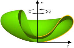
Figure 1: (color online) Example of an axisymmetric shell with coordinates $z$, $r$, and $\varphi$. The shell is generated by revolution of the generatrix (orange thin line) that is calculated by the shape equations.

We work in cylindrical coordinates to directly exploit the axisymmetry. The axis of symmetry is called $z$, the distance to this axis $r$, and the polar angle $\varphi$, see Fig. 1. The shell is given by the generatrix $[r(s),z(s)]$ which is parametrized in arc length $s$ (starting at the lower apex with $s=0$ and ending at the upper apex with $s=L$). The unit tangent vector $\mathbf{e}_{s}$ to the generatrix at $[r(s),z(s)]$ defines an angle $\psi$ via $\mathbf{e}_{s}=(\cos\psi,\sin\psi)$, which can be used to quantify the orientation of a patch of the capsule relative to the axis of symmetry.

II.2 Hydrodynamics

We want to calculate the flow field of a viscous incompressible fluid around an axisymmetric capsule of given fixed shape. For the calculation of the flow field the deformability of the capsule is not relevant, and the capsule can be viewed as a general immersed body of revolution $B$. For the calculation of the capsule shape and the determination of its sedimenting velocity, we only need to calculate the surface forces onto the capsule which are generated by the fluid flow.

In the limit of small Reynolds numbers the stress tensor $\sigma$ in a stationary fluid on which no external body forces are exerted is given by the stationary Stokes equation Happel and Brenner (1983)

$$\nabla\cdot\sigma=0\text{.}$$ (1)

In Cartesian coordinates, the stress tensor is given by $\sigma_{ij}=-p\delta_{ij}+2\mu e_{ij}$, where $p$ is the hydrodynamic pressure, $\mu$ the viscosity, and $e_{ij}=\left({\partial_{j}u_{i}}+{\partial_{i}u_{j}}\right)/2$ is the rate of deformation tensor for a fluid velocity field $\mathbf{u}$. Additionally, for an incompressible fluid, the continuity equation $\nabla\cdot\mathbf{u}=0$ holds. From the stress tensor one can infer the surface force density $\mathbf{f}=\sigma\cdot\mathbf{n}$ onto the capsule by means of the local surface normal $\mathbf{n}$.

In the rest frame of the sedimenting axisymmetric capsule and with a “no-slip” condition at the capsule surface $\partial B$, we are looking for axisymmetric solutions that have a given flow velocity $\mathbf{u}^{\infty}$ at infinity and vanishing velocity on the capsule boundary. In the laboratory frame, $-\mathbf{u}^{\infty}$ is the sedimenting velocity of the capsule in the stationary state. Therefore, $\mathbf{u}^{\infty}$ has to be determined by balancing the total gravitational pulling force and the total hydrodynamic drag force on the capsule.

In the laboratory frame we are looking for solutions with vanishing pressure and velocity at infinity. The Green’s function for these boundary conditions is the well-known Stokeslet (also called Oseen-Burgers tensor), that is, the fluid velocity $\mathbf{u}$ at $\mathbf{y}$ due to a point-force $-\mathbf{F}_{p}$ acting on the fluid at $\mathbf{x}$,

$$\mathbf{u}(\mathbf{y})=-\frac{1}{8\uppi\mu}\mathsf{G}(\mathbf{y}-\mathbf{x})\cdot\mathbf{F}_{p}$$ (2)

with the Stokeslet $\mathsf{G}$ whose elements are in Cartesian coordinates ($x\equiv\lvert\mathbf{x}\rvert$)

$$\mathsf{G}_{ij}(\mathbf{x})=\frac{\delta_{ij}}{x}+\frac{x_{i}x_{j}}{x^{3}}\text{.}$$ (3)

This is the basis of the boundary integral approach for a solution of the Stokes equation, where we want to find the correct distribution of point forces to match the “no-slip” condition on the capsule surface.

Because of the axisymmetry we can integrate over the polar angle and find the velocity due to a ring of point forces with a local force density $-\mathbf{f}$ acting on the fluid, $\mathbf{u}(\mathbf{y})=-\frac{1}{8\uppi\mu}\mathsf{M}(\mathbf{y},\mathbf{x})\cdot\mathbf{f}$, with a matrix $\mathsf{M}$, which can be calculated by integration of the Stokeslet $\mathsf{G}$ with respect to the polar angle. Switching from forces $-\mathbf{f}$ acting on the fluid to forces $\mathbf{f}$ acting on the capsule and integrating over all point forces on the surface, we find the general solution of the Stokes equation for an axisymmetric point force distribution on the surface of the body of revolution $B$,

$$u_{\alpha}(\mathbf{y})=-\frac{1}{8\uppi\mu}\int_{C}\mathrm{d}s(\mathbf{x})\mathsf{M}_{\alpha\beta}(\mathbf{y},\mathbf{x})f_{\beta}(\mathbf{x})\text{.}$$ (4)

Here Greek indices denote the component in cylindrical coordinates, i.e., $\alpha,\beta=r,z$ ($u_{\varphi}=f_{\varphi}=0$ for symmetry reasons). For these coordinates, the elements of the matrix kernel $\mathsf{M}$ are given in Appendix A according to Ref. 8. The integration in (4) runs along the path $C$ given by the generatrix, i.e., the cross section of the boundary $\partial B$, with arc length $s(\mathbf{x})$. This representation of a Stokes flow in terms of a single-layer potential (using only the Stokeslet and not the stresslet) is possible as long as there is no net flow through the surface of the capsule

$$\int\mathrm{d}A\,(\mathbf{u}-\mathbf{u}_{0})\cdot\mathbf{n}=0\text{.}$$ (5)

According to the “no-slip” condition we have (working in the laboratory frame) $\mathbf{u}=-\mathbf{u}^{\infty}$ at every point $\mathbf{y}\in\partial B$ on the surface. This results in the equation

$$u_{\alpha}^{\infty}=\frac{1}{8\uppi\mu}\int_{C}\mathrm{d}s(\mathbf{x})\mathsf{M}_{\alpha\beta}(\mathbf{y},\mathbf{x})f_{\beta}(\mathbf{x})~{}~{}(\mbox{for}~{}\mathbf{y}\in\partial B),$$ (6)

which can be used to determine the surface force distribution.

To numerically solve the integral for the surface force $f(\mathbf{x}_{i})$ at a given set of points $\{\mathbf{x}_{i}\}$ ($i=1,\ldots,N$) we employ a simple collocation method, i.e., we choose a discretized representation of the function $f_{\beta}(\mathbf{x})$ and approximate the integral in (6) by the rectangle method. This leads to a system of linear equations

$$\mathbf{U}=\tilde{\mathsf{M}}\mathbf{F}$$ (7)

with the “super-vectors”

$$\mathbf{U} = (u^{\infty}(\mathbf{y}_{1})_{r},u^{\infty}(\mathbf{y}_{1})_{z},\ldots,u^{\infty}(\mathbf{y}_{N})_{r},u^{\infty}(\mathbf{y}_{N})_{z})$$ (8)

$$= (0,u^{\infty},\ldots,0,u^{\infty})$$

$$\mathbf{F} = (f(\mathbf{x}_{1})_{r},f(\mathbf{x}_{1})_{z},\ldots,f(\mathbf{x}_{N})_{r},f(\mathbf{x}_{N})_{z})$$ (9)

and a matrix (using numbered indices $r\widehat{=}0$, $z\widehat{=}1$ for a more compact notation)

$$\tilde{\mathsf{M}}_{2i+\alpha-1,2j+\beta-1}=\frac{1}{8\uppi\mu}(s(\mathbf{x}_{j+1})-s(\mathbf{x}_{j}))\mathsf{M}_{\alpha\beta}(\mathbf{y}_{i},\mathbf{x}_{j}).$$ (10)

Due to singularities in the diagonal components of $\mathsf{M}$, the two sets of points $\{\mathbf{x}_{i}\},\{\mathbf{y}_{i}\}$ must be distinct (or $\mathsf{M}$ otherwise regularized), so $2N$ points on the surface are needed, and the solution is the surface force at points $\{\mathbf{y}_{i}\}$. We validate our regularization in Appendix B. For use in the shape equations, we then decompose this surface force into one component acting normal to the surface, the hydrodynamic pressure $p_{n}$, and another component acting tangential to the surface, the shear pressure $p_{s}$ (see Fig. 3).

We note that we usually restrict our computations to the bare minimum, i.e., the surface forces needed for the calculation of the capsule shape but, thereby, have all necessary information to reconstruct the whole velocity field in the surrounding liquid as shown in Fig. 2.

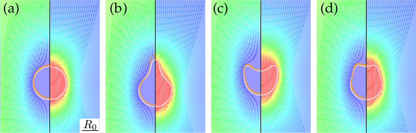
Figure 2: (Color online) Fluid velocity field around the four stationary capsule shapes under volume control, (a) pseudospherical, (b) pear shape, (c) strongly buckled, and (d) weakly buckled, in the capsule resting frame (left halves) and in the laboratory frame (right halves). The sedimenting force acts downwards, and arrows indicate the direction of flow. The arrows are equidistant in time, so a higher arrow density along a line represents a lower velocity. Additionally, the absolute value of the velocity is color coded in the background and the hydrodynamic surface forces are shown with arrows on the surface. The scale is identical in panels (a)-(d) and given by the scale bar of length $R_{0}$ in (a).

Throughout this paper, we use a “no-slip” condition, that is, the velocity directly at the surface of the immersed body vanishes in its resting frame. It is possible, however, to extend this boundary integral approach to incorporate a prescribed velocity field on the surface in the resting frame of the capsule Pozrikidis (1992). This will allow us to generalize the approach to model active swimmers Lauga and Powers (2009); Degen (2014) in future work.

II.3 Equilibrium shape of capsule

The sedimenting capsule is deformed by the hydrodynamic stresses from the surrounding fluid. We calculate the equilibrium shape of the capsule by a set of shape equations, which have been derived in Refs. 37; 38. We generalize these shape equations to include the additional fluid stresses on the capsule, which we obtain as the surface force density components $f_{r}$ and $f_{z}$ from the hydrodynamic flow as described in the previous section. In order to make our approach self-consistent, the capsule shape $B$ from which hydrodynamic surface forces are calculated has to be identical to the capsule shape that is obtained by integration of the shape equation under the influence of these hydrodynamic surface forces. This is achieved by an iterative procedure, which will be explained in the following section.

The shape of a thin axisymmetric shell of thickness $H$ can be derived from non-linear shell theory Libai and Simmonds (1998); Pozrikidis (2003). A known reference shape $[r_{0}(s_{0}),z_{0}(s_{0})]$ (a subscript zero refers to a quantity of the reference shape; $s_{0}\in[0,L_{0}]$ is the arc length of the reference shape) is deformed by hydrodynamic forces exerted by the viscous flow. Each point $[r_{0}(s_{0}),z_{0}(s_{0})]$ is mapped onto a point $[r(s_{0}),z(s_{0})]$ in the deformed configuration, which induces meridional and circumferential stretches, $\lambda_{s}=ds/ds_{0}$ and $\lambda_{\varphi}=r/r_{0}$, respectively. The arc length element $ds$ of the deformed configuration is $ds^{2}=[r^{\prime}(s_{0})^{2}+z^{\prime}(s_{0})^{2}]ds_{0}^{2}$.

The shape of the deformed axisymmetric shell is given by the solution of a system of first-order differential equations, henceforth referred to as the shape equations. Using the notation of Refs. 37; 38 these can be written as

$$r^{\prime}(s_{0}) = \lambda_{s}\cos{\psi}~{},~{}~{}z^{\prime}(s_{0})=\lambda_{s}\sin{\psi}~{},~{}~{}\psi^{\prime}(s_{0})=\lambda_{s}\kappa_{s}$$

$$\tau^{\prime}_{s}(s_{0}) = \lambda_{s}\left(\frac{\tau_{\varphi}-\tau_{s}}{r}\cos\psi+\kappa_{s}q+p_{s}\right)$$

$$m^{\prime}_{s}(s_{0}) = \lambda_{s}\left(\frac{m_{\varphi}-m_{s}}{r}\cos\psi-q+l\right)$$

$$q^{\prime}(s_{0}) = \lambda_{s}\left(-\kappa_{s}\tau_{s}-\kappa_{\varphi}\tau_{\varphi}-\frac{q}{r}\cos\psi+p\right)\text{.}$$ (11)

The additional quantities appearing in these shape equations are shown in Fig. 3 and defined as follows: The angle $\psi$ is the slope angle between the tangent plane to the deformed shape and the $r$ axis, $\kappa_{\varphi}$ is the circumferential curvature, $\kappa_{s}$ the meridional curvature. The meridional and circumferential stresses are denoted by $\tau_{s}$ and $\tau_{\varphi}$, respectively; $q$ is the transverse shear stress, $p$ the total normal pressure, $p_{s}$ the shear pressure, and $l$ the external stress couple.

The first three of the shape equations (11) follow from geometry, the last three equations express force and moment equilibrium. For a derivation of these equations we refer to Refs. 39; 40; 37. In order to close the Eqs. (11), additional geometrical relations

$$\kappa_{\varphi}=\frac{\sin\psi}{r}~{},~{}~{}\kappa_{s}=\frac{d\psi}{ds}~{},~{}~{}\lambda_{\varphi}=\frac{r}{r_{0}}$$ (12)

and constitutive stress-strain relations that depend on the elastic law governing the shell material are needed. The elastic law will be discussed in the following paragraph.

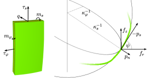
Figure 3: (Color online) Left: Tensions and bending moments acting on a shell segment (thickness $H$). Right: Part of the generatrix (green thick line) with the decomposition of external surface force densities into the coordinate components ($f_{r}$, $f_{z}$) as well as into normal and tangent components ($p_{n}$, $p_{s}$). Also shown are the two principal curvature radii $\kappa_{s}^{-1}$ and $\kappa_{\varphi}^{-1}$ with corresponding osculating circles.

The normal pressure

$$p=p_{0}+p_{n}-g_{0}\Delta\rho z$$ (13)

(i.e., the pressure difference $p\equiv p_{\rm in}-p_{\rm out}$ between inside and outside pressure), the shear-pressure $p_{s}$, and the stress couple $l=p_{s}H/2$ (the fluid inside the capsule is at rest) are given externally by hydrodynamic and external driving forces; $g_{0}$ is the gravitational acceleration and $\Delta\rho=\rho_{\rm in}-\rho_{\rm out}$ the density difference between the fluids inside and outside the capsule. Note that we measure the gravitational hydrostatic pressure $-g_{0}\Delta\rho z$ relative to the lower apex, for which we can always choose $z(0)=0$.

The pressures $p_{n}$ and $p_{s}$ are the normal and tangential forces per area, which are generated by the surrounding fluid. The surface force density vector $\mathbf{f}=f_{z}\mathbf{e}_{z}+f_{r}\mathbf{e}_{r}$, which has been calculated in the previous section, can also be expressed in terms of $p_{n}$ and $p_{s}$, $\mathbf{f}=p_{n}\mathbf{n}-p_{s}\mathbf{e}_{s}$ ($\mathbf{n}$ and $\mathbf{e}_{s}$ are normal and tangent unit vectors to the generatrix). Using the decompositions $\mathbf{n}=-\cos\psi\mathbf{e}_{z}+\sin\psi\mathbf{e}_{r}$ and $\mathbf{e}_{s}=\sin\psi\mathbf{e}_{z}+\cos\psi\mathbf{e}_{r}$ with the slope angle $\psi$, we find:

$$p_{n} =\mathbf{f}\cdot\mathbf{n}=f_{r}\sin\psi-f_{z}\cos\psi$$ (14)

$$p_{s} =-\mathbf{f}\cdot\mathbf{e}_{s}=-f_{r}\cos\psi-f_{z}\sin\psi\text{.}$$ (15)

This is also illustrated in Fig. 3.

All remaining quantities in the shape equations (11) follow from constitutive (stress-strain) relations that depend on the elastic law, which will be discussed in the following paragraph. In addition to the elastic law, there might be global constraints. We consider here only one geometric constraint to the shape, namely a fixed volume $V=V_{0}$ (due to an incompressible fluid inside the closed capsule). We introduce the conjugated Lagrange parameter $p_{0}$, the static pressure difference between the interior and exterior fluids, which also enters the pressure $p$ in Eq. (13). Additionally, the shape has to be in global force equilibrium, to which the velocity of the capsule is the conjugated parameter.

II.3.1 Elastic law and reference shapes

Within this work we use a Hookean energy density with a spherical resting shape to model deformable capsules. As a measure for the deformation of the capsule we introduce the meridional and circumferential strains

$$e_{s}=\lambda_{s}-1~{},~{}~{}e_{\varphi}=\lambda_{\varphi}-1$$ (16)

as well as the meridional and circumferential bending strains

$$K_{s}=\lambda_{s}\kappa_{s}-{\kappa_{s}}_{0}~{},~{}~{}K_{\varphi}=\lambda_{\varphi}\kappa_{\varphi}-{\kappa_{\varphi}}_{0}\text{.}$$ (17)

The elastic energy we use is Hookean, i.e., a quadratic form in these strains. More precisely, the surface energy density $w$, which measures the elastic energy of an infinitesimal patch of the (deformed) surface divided by the area of this patch in the undeformed state, is given by

$$w_{s} = \frac{1}{2}\frac{Y_{\rm 2D}}{1-\nu^{2}}\left(e_{s}^{2}+2\nu e_{s}e_{\varphi}+e_{\varphi}^{2}\right)$$ (18)

$$+\frac{1}{2}E_{B}\left(K_{s}^{2}+2\nu K_{s}K_{\varphi}+K_{\varphi}^{2}\right)$$

with the two-dimensional Young modulus $Y_{\rm 2D}$, which defines the tension (energy per surface) scale, the bending modulus $E_{B}$ and the (two-dimensional) Poisson ratio $\nu$ (assuming equal Poisson ratios for bending and stretching). The fundamental length scale is the radius $R_{0}$ of the spherical rest shape (with $R_{0}={\kappa_{s}}_{0}^{-1}$ and $L_{0}=\uppi R_{0}$). Tensions and bending moments derive from the surface energy (18) by $\tau_{s}=\lambda_{\varphi}^{-1}\partial w/\partial e_{s}$ and $K_{s}=\lambda_{\varphi}^{-1}\partial w/\partial K_{s}$ (and two more analogous relations with indices $s$ and $\varphi$ interchanged), which gives the missing constitutive stress-strain relations for the shape equations (11). For Hookean elasticity and a spherical rest shape, the resulting set of shape equations has been solved for a purely hydrostatic pressure $p=p_{0}$ and $p_{s}=0$ in Ref. 37.

The Hookean elastic model for a spherical rest shape contains five parameters, $Y_{\rm 2D}$, $R_{0}$, $E_{B}$, $\nu$, and $H$, characterizing capsule size and elastic properties. In Sec. III.1 below, we will eliminate two parameters, $Y_{\rm 2D}$ and $R_{0}$, by choosing our scales of energy (or tension) and length appropriately. The two-dimensional Poisson ratio is bounded by $\nu\in[-1;1]$, and we reduce our parameter space by always using $\nu=1/2$. This way our Hookean energy density has the same behavior for small stresses as the more complex Mooney-Rivlin functional Libai and Simmonds (1998). The thickness $H$ enters the shape equations only via the stress couple $l$ and, thus, only weakly influences the resulting shape. Assuming that the shell can be treated as a thin shell made from an isotropic elastic material, the bending modulus is directly related to the shell thickness $H$ by

$$E_{B}=\frac{Y_{\rm 2D}H^{2}}{12(1-\nu^{2})}=\frac{1}{9}Y_{\rm 2D}H^{2}\text{.}$$ (19)

Thus, we have one remaining free parameter to change the elastic properties, the bending modulus $E_{B}$.

The Hookean elastic energy law we use here is well suited to describe the deformation behavior of soft elastic capsules. For other systems different energies might be more adequate (e.g. Helfrich bending energy and a locally inextensible surface for vesicles). As pointed out above, a different choice of elastic law enters the formalism through the constitutive relations and, thus, does not require changes in our method on the conceptual level.

II.3.2 Solution of the shape equations

The boundary conditions for a shape that is closed and has no kinks at its poles are

$$r(0)=r(L_{0})=\psi(0)=\uppi-\psi(L_{0})=0,$$ (20)

and we can always choose $z(0)=0$. For the solution of the shape equations it is important that there is no net force on the capsule as the shape equations are derived from force equilibrium. The condition that the total hydrodynamic drag force equals the total gravitational force determines the resulting sedimenting velocity. If hydrodynamic drag and gravitational pull cancel each other in a stationary state, there is no remaining point force at the poles needed to ensure equilibrium and, thus,

$$q(0)=q(L_{0})=0\text{.}$$ (21)

The shape equations have (removable) singularities at both poles; therefore, a numerical solution has to start at both poles requiring $12$ boundary conditions ($r,z,\psi,\tau,m,q$ at both poles), from which we know $7$ [by Eqs. (20) and (21) and $z(0)=0$]. The $5$ remaining parameters can be determined by a shooting method using that the solution starting at $s_{0}=0$ and the one starting at $s_{0}=L_{0}$ have to match continuously in the middle, which gives $6$ matching conditions ($r,z,\psi,\tau,m,q$). This gives an overdetermined nonlinear set of equations which we solve iteratively using linearizations. However, as in the static case Knoche and Kierfeld (2011), the existence of a solution to the resulting system of linear equations (the matching conditions) is ensured by the existence of a first integral (see Appendix C) of the shape equation. In principle, this first integral could be used to cancel out the matching condition for one parameter (e.g., $q$), and, thus, we have $5$ independent equations to determine $5$ parameters, and the system is not genuinely overdetermined. We found the approach using an overdetermined system to be better numerically tractable, where we ultimately used a multiple shooting method including several matching points between the poles. Throughout this work we used a fourth-order Runge-Kutta scheme with step width $\Delta s_{0}=5\times 10^{-5}R_{0}$.

Using these boundary conditions, it is straightforward to see that the shape equations do not allow for a solution whose shape is the reference shape, unless there are no external loads ($p_{s}=p=l=0$). There will be solutions arbitrarily close to a sphere, which we call pseudospherical.

II.4 Iterative solution of shape and flow and determination of sedimenting velocity

Figure 4: Iterative scheme for the solution to the problem of elastic capsules in Stokes flow as explained in the text.

We find a joint solution to the shape equations and the Stokes equation by solving them separately and iteratively, as illustrated in the scheme in Fig. 4, to converge to the desired solution: We assume a fixed axisymmetric shape and calculate the resulting hydrodynamic forces on the capsule for this shape. Then, we use the resulting hydrodynamic surface force density to calculate a new deformed shape. Using this new shape we re-calculate the hydrodynamic surface forces and so on. We iterate until a fixed point is reached. At the fixed point, our approach is self-consistent, i.e., the capsule shape from which hydrodynamic surface forces are calculated is identical to the capsule shape that is obtained by integration of the shape equation under the influence of exactly these hydrodynamic surface forces.

For each capsule shape during the iteration, we can determine its sedimenting velocity $u=|\mathbf{u}^{\infty}|$ by requiring that the total hydrodynamic drag force equals the total gravitational force,

$$g_{0}\Delta\rho V_{0}=-\int_{C}\mathrm{d}s(\mathbf{x})2\uppi r(\mathbf{x})f_{z}(\mathbf{x})$$ (22)

The integration runs along the path $C$ given by the generatrix, i.e., the cross section of the boundary $\partial B$, with arc length $s(\mathbf{x})$. By changing $u=|\mathbf{u}^{\infty}|$ we can adjust the hydrodynamic drag forces on the right hand side to achieve equality for a given capsule shape during the iteration. During the iteration $u$ will converge to the proper sedimenting velocity for the stationary state.

The Stokes equation is linear in the velocity, and we can just scale the resulting surface forces accordingly, if we change the velocity parameter $u^{\infty}$. In this way, the global force balance can be treated the same way as other possible constraints like a fixed volume. Numerically, it is impossible to ensure the exact equality of the drag and the drive forces in Eq. (22). Demanding a very small residual force difference makes it difficult to find an adequate velocity, and a too-large force difference makes it impossible to find a solution with small errors at the matching points. Global force balance (22) is equivalent to the condition that the total force in axial direction vanishes,

$$X(L)=-2\uppi\int_{0}^{L}\mathrm{d}s\,r(p\cos\psi+p_{s}\sin\psi)=0\text{,}$$ (23)

see Eqs. (13) and (15) and Fig. 3. Interestingly, the total axial force is directly related to the existence of a first integral of the shape equations, which is discussed in the Appendix C, see Eq. (48). To monitor global force balance numerically, we use a criterion $\lvert X(L)\rvert<10^{-5}$, which turns out to be a good compromise for a numerical force balance criterion.

The iteration starts with a given (arbitrary) stress, e.g., one corresponding to the flow around the reference shape. For the resulting initial capsule shape, the Stokes flow is computed and the resulting stress is then used to start the iteration. If, during the iteration, the new and old stress differ strongly it might be difficult to find the new shooting parameters for the capsule shape and the right sedimenting velocity starting at their old values. To overcome this technical problem, we use a convex combination $\sigma=\alpha\sigma_{\text{new}}+(1-\alpha)\sigma_{\text{old}}$ of the two stresses and slowly increase the fraction $\alpha$ of the new stress until it reaches unity. The iteration continues until the change (monitored in pressure and velocity) within one iteration cycle is sufficiently small. In total, this allows for a joint solution of the shape equations and the Stokes equation to find the stationary shape and the sedimenting velocity at rather small numerical cost.

If there are multiple stationary solutions at a given gravitational strength (see discussion of the shape diagram 5 in Sec. III.2 below), the iterative procedure obviously converges to only one shape. Which stationary shape is selected depends on the initial configuration. A stationary shape can be continuated to different parameter values by slightly changing the control parameters and using the former stationary shape as new initial shape.

In order to find all branches of stationary shapes we first generate capsule shapes for a fixed (artificial) flow field for the whole range of gravitational fields at a fixed bending rigidity. These serve as initial shapes from which we iterate until a stationary shape with the correct flow field is reached. At low bending rigidities, this procedure generates (all four) different classes of stationary shapes depending on the gravitational force. We then try to continuate all different classes of stationary shapes to the whole range of gravitational forces and, afterwards, to the whole range of bending rigidities. This allows us to obtain a full set of solutions and identify all different branches.

III Results

In this section we present the results for stationary axisymmetric sedimenting shapes and stationary sedimenting velocities as obtained by the fixed point iteration method. We focus on the sedimentation of capsules under volume control ($V=V_{0}=\text{const}$) in the main text and present additional results for pressure control ($p_{0}=\text{const}$) in Appendix E. Additionally, we show the results for a capsule that is driven (or pulled) by a localized point force rather than a homogeneous body force.

III.1 Control parameters and non-dimensionalization

In order to identify the relevant control parameters and reduce the parameter space, in the remainder of the paper we introduce dimensionless quantities by measuring lengths in units of the radius $R_{0}$ of the spherical rest shape of the capsule, energies in units of $Y_{\rm 2D}R_{0}^{2}$ (i.e., tensions in units of $Y_{\rm 2D}$), and times in units of $R_{0}\mu/Y_{\rm 2D}$. This results in the following set of control parameters for the capsule shape:

1. Our elastic law is fully characterized by the dimensionless bending modulus or its inverse, the Föppl-von-Kármán number Libai and Simmonds (1998),

   $$\tilde{E}_{B}\equiv\frac{E_{B}}{Y_{\rm 2D}R_{0}^{2}}=\frac{1}{\gamma_{\rm FvK}}.$$ (24)

   In general, elastic properties also depend on the Poisson ratio $\nu$ but we limit ourselves to $\nu=1/2$ as explained above. Using the thin-shell result (19) the dimensionless bending modulus $\tilde{E}_{B}=(H/9R_{0})^{2}$ also determines the shell thickness $H$ for an isotropic shell material.

2. The sedimentation motion of the capsule is determined by the strength of the gravitational (or centrifugal) pull $g_{0}\Delta\rho$ (the gravitational force density), which we measure in units of $Y_{\rm 2D}/R_{0}^{2}$ in the following. The dimensionless gravitational force $g$ then takes the form of a Bond number,

   $$g={\mathrm{B}o}\equiv\frac{g_{0}\Delta\rho R_{0}^{2}}{Y_{\rm 2D}},$$ (25)

   where the characteristic elastic tension $Y_{\rm 2D}$ is used instead of a liquid surface tension.

3. The static pressure $p_{0}$ within the capsule is measured in units of $Y_{\rm 2D}/R_{0}$ in the following.

4. The resulting sedimenting velocity $u$ is measured in units of $Y_{\rm 2D}/\mu$.

We conclude that the resulting stationary sedimenting shapes of the capsule are fully determined by two dimensionless control parameters if the capsule volume is fixed: (i) dimensionless bending modulus $\tilde{E}_{B}$ or its inverse, the Föppl-von-Kármán number $\gamma_{\rm FvK}=1/\tilde{E}_{B}$ characterizes the elastic properties of the capsule (by the typical ratio of bending to stretching energy) and (ii) the Bond number describes the strength of the driving force (relative to elastic deformation forces). If the capsule pressure is controlled rather than its volume, the dimensionless pressure $p_{0}$ provides a third parameter, see Appendix E. Because stationary shapes are independent of time, they do not depend on the solvent viscosity.

III.2 Shape diagram

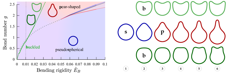
Figure 5: (Color online) Left: Stationary axisymmetric shapes for a sedimenting Hookean capsule with spherical reference shape in the parameter plane of the two control parameters, the dimensionless bending modulus $\tilde{E}_{B}$ (the inverse of the Föppl-von-Kármán number $\gamma_{\rm FvK}$) and the dimensionless gravity $g$ (the Bond number $\mathrm{Bo}$). We find pseudospherical (blue), pear-shaped (red), and a pair of strongly (light green) and weakly (dark green) buckled shapes. The black line is a line of discontinuous shape transitions between pear and pseudospherical shape which terminates in a critical point beyond which a sphere transforms smoothly into the pear shape. The blue and red lines are spinodals indicating the limits of stability of the pseudospherical and pear-shaped shapes, respectively. Above the solid green line the pair of buckled shapes occur in a bifurcation; the dotted continuation of the solid line signals numerical difficulties in following this bifurcation line. To which solution the iteration procedure converges in regions with shape coexistence is controlled by the initial conditions. Right: Contours of all four types of shapes for $\tilde{E}_{B}=0.01$, i.e., along the vertical black dotted line, in the range $g=0.7~{}\text{to}~{}1.7$. The gravity strength $g$ increases from left to right in steps of $\Delta g=0.2$.

The spherical rest shape has a dimensionless volume $V=4\uppi/3$. For sedimentation under volume control, we use this as the fixed volume $V_{0}=4\uppi/3$. In principle, it is also possible to prescribe volumes that differ from the rest shape volume. This can be done using pressure control, for which we present results in Appendix E. For the static case, the only stationary shape at fixed volume is the strictly spherical shape, regardless of the bending modulus. This differs for a sedimenting capsule, which displays various shape transitions already at fixed volume.

We summarize our findings regarding the axisymmetric sedimenting shapes in the shape diagram Fig. 5 in the $(\tilde{E}_{B},g)$ plane of the two control parameters. We investigated stationary axisymmetric capsule shapes for gravity strengths (Bond numbers) up to $g=g_{\text{max}}=2.5$ (usually using steps of $\Delta g=0.005$) and bending moduli $\tilde{E}_{B}=10^{-3}~{}\text{to}~{}10^{-1}$ corresponding to Föppl-von-Kármán numbers $\gamma_{\rm FvK}=10~{}\text{to}~{}1000$. For high Bond and Föppl-von-Kármán numbers, the iteration procedure becomes numerically more demanding (higher forces ask for finer discretization of the shape equations, smaller distances between solutions in parameter space ask for a more thorough fixed point search), but remains possible in principle. We will discuss further below in detail, which parameter regimes in the $(\tilde{E}_{B},g)$ plane are accessible for different types of capsules and sedimenting driving forces.

Overall, we identify three classes of axisymmetric shapes, which are shown in Fig. 2:

1. Pseudospherical shapes, which remain convex and close to the rest shape. For pseudospherical shapes the velocity is still given by the result for a perfect sphere, which is Stokes’ law $u\approx F/6\uppi\approx 2g/9$ (in dimensionless form), to a good approximation. Likewise, the pressure due to gravity is $p_{0}\approx g\langle z\rangle\approx g$.

2. Pear shapes, which have a convex upper apex but develop an axisymmetric indentation at the side of the capsule. For high gravitational driving force (high sedimentation velocities) the pear shape resembles a tether with a high curvature at the upper apex.

3. Buckled shapes, which develop a concave axisymmetric indentation at the upper apex of the capsule. For fixed capsule volume, these buckled shapes always occur in pairs of a weakly buckled shape with a shallow and narrow indentation and a strongly buckled shape with a deep and wide indentation at the upper apex.

Our solution method allows us to identify all bifurcations or transitions between these classes of shapes as shown in Fig. 5. Upon increasing the gravity $g$ or decreasing the bending rigidity $\tilde{E}_{B}$, the stationary sedimenting pseudospherical shape transforms into a pear shape. The black line in Fig. 5 is a line of discontinuous shape transitions between pseudospherical and pear shape, which terminates in a critical point at

$$g_{c}\simeq 1.85~{}\mbox{and}~{}\tilde{E}_{B,c}\simeq 0.05.$$ (26)

At the discontinuous shape transition we find hysteresis with two spinodal lines (red and blue lines) indicating the limits of stability of pseudospherical and pear-shape shapes. For smaller bending rigidities $\tilde{E}_{B}<\tilde{E}_{B,c}$, the spherical shape transforms smoothly into the pear shape upon increasing gravity. We locate the transition lines between the sphere and pear shape by the condition of equal sedimenting velocity (for the discontinuous transition) or maximal sedimenting velocity (for the smooth crossover) as explained in the next section. Discontinuous buckling transitions are also known from static spherical shells Landau and Lifshitz (1986); Pogorelov (1988), for example, as a function of the external static pressure or an osmotic pressure Knoche and Kierfeld (2014). That a line of discontinuous buckling transitions terminates in a critical point as a function of the elastic properties of the capsules is, however, an unknown phenomenon for static buckling transitions.

Within the smooth crossover regime between sphere and pear shapes at small bending rigidities $\tilde{E}_{B}<\tilde{E}_{B,c}$, the pair of stationary buckled shapes occurs in a bifurcation upon increasing the gravity strengths $g$ above a critical threshold given by the solid green line in Fig. 5. Also the spherical or pear shape remains a stable solution above the green line, such that we have three possible stationary sedimenting shapes in this parameter regime. Which of these shapes is dynamically selected in an actual experiment, depends on the initial conditions. The dotted continuation of the solid green line signals numerical difficulties in following this bifurcation line.

The iterative method allows us to determine stationary sedimenting shapes in the shape diagram Fig. 5 very efficiently. In order to continuate the branch of pseudospherical and pear-shaped solutions for a fixed bending rigidity $\tilde{E}_{B}=0.01$ in Bond number steps of $\Delta g=0.005$ in the range $g=0,...,2$, we need a computing time of approximately 6 h on a four core Intel Xeon processor (3.7 GHz).

III.3 Force-velocity relation

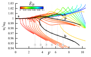
Figure 6: (Color online) Force-velocity relations for sedimenting capsules under volume control. The plot shows the velocity relative to the (dimensionless) velocity $u_{0}=2g/9$ of a perfect sphere with the same volume (Stokes’ law) as a function of the (dimensionless) total external force $F=4\uppi g/3$. The bending modulus $\tilde{E}_{B}$ is color coded. Two distinct branches can be distinguished: The solution branches corresponding to pseudospherical and pear shapes start at zero force. A pair of solution branches for strongly or weakly buckled shapes starts at a nonzero threshold force. The branches for $\tilde{E}_{B}=0.01$ are marked in black as a typical example. The capsule shapes 1–6 in Fig.  5 are realized at the points marked by circles. It is also apparent that the transition from pseudospherical to pear shapes is continuous for $\tilde{E}_{B}\lessapprox 0.05$ and becomes discontinuous for $\tilde{E}_{B}\gtrapprox 0.05$.

All dynamic shape transitions reflect in bifurcations in the force-velocity relations. In Fig. 6, we show the force-velocity relations between sedimenting velocity $u$ and gravity $g$ for all stationary axisymmetric shapes and for a color-coded range of bending rigidities $\tilde{E}_{B}=10^{-3}~{}\text{to}~{}10^{-1}$. The total driving force $F$ can be computed using the total drag from the fluid corresponding to the right hand side of Eq.  (22) or as the product of the total mass difference and the sedimenting acceleration $F=g_{0}\Delta\rho V_{0}$ or $F=4\uppi g/3$ (in dimensionless form) corresponding to the left-hand side of Eq. (22). The leading contribution of the force-velocity relation is given by the force-velocity relation of a perfect sphere, which is Stokes’ law $u=u_{0}=F/6\uppi=2g/9$ (in dimensionless form). To eliminate this leading contribution, we show the relative velocity $u/u_{0}$ in Fig. 6. By definition, the relative velocity is also proportional to the sedimentation coefficient, which is defined as $v/g_{0}$ and a standard quantity in centrifugation and sedimentation experiments Planken and Cölfen (2010).

Figure 6 clearly shows two qualitatively different types of force-velocity curves. The force-velocity curves corresponding to pseudospherical or pear shapes with positive curvature at both apexes start at zero force, whereas the solution curves corresponding to the weakly and strongly buckled shapes bifurcate at a nonzero threshold force with a vertical tangent and have two branches: The weakly buckled shapes with a narrow indentation have a higher sedimenting velocity and correspond to the upper branch, and the strongly buckled shapes have a lower sedimenting velocity and correspond to the lower branch.

We note that, because of the $g$ dependence of $u_{0}$, the absolute sedimenting velocities $u$ are increasing with increasing gravity for both buckled shapes, although $u/u_{0}$ is decreasing for the strongly buckled shapes. Above the threshold force for the buckled shapes, three different axisymmetric sedimenting capsule shapes can occur with different sedimenting velocities for the same gravitational driving force. Which of these shapes is dynamically selected in an actual experiment, depends on the initial conditions.

The force-velocity curves for the pseudospherical or pear shapes allow us to detect how the transition between spherical and pear shapes evolves into a discontinuous transition: Figure 6 shows that these force-velocity curves develop a cusp close to the critical point for $\tilde{E}_{B}\approx E_{B,c}\simeq 0.05$, whereas they remain smooth for $\tilde{E}_{B}<E_{B,c}$. For $\tilde{E}_{B}>E_{B,c}$, we find two overlapping and intersecting velocity branches, which corresponds to the characteristic hysteretic velocity switching in a discontinuous transition. In fact, we identify the discontinuous transition line in Fig. 5 by these velocities: If the two branches coexist, then we localize the transition at the crossing of the two $u(g)$ curves. For $\tilde{E}_{B}<E_{B,c}$, the velocity curve still exhibits a maximum, which we can use to define the crossover line between the pseudospherical and pear shape as it is shown in the shape diagram Fig. 5. The discontinuous nature of the sphere-pear transition is confirmed by monitoring other quantities, such as the capsule area, as a function of the gravity $g$. As illustrated in Fig. 7, the area clearly exhibits hysteretic switching at the transition. The pair of weakly and strongly buckled solutions appears in a bifurcation above a critical driving force. Also this bifurcation reflects in a corresponding bifurcation of the capsule area as shown in the inset of Fig. 7.

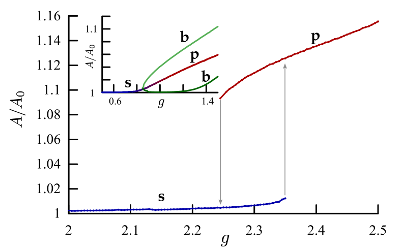
Figure 7: (Color online) Reduced capsule area as a function of the dimensionless gravity strength $g$ for a high bending modulus $\tilde{E}_{B}=0.08$. There is an interval where pseudospherical and pear-shaped solutions with different area coexist with hysteretic switching upon increasing and decreasing $g$. Inset: For $\tilde{E}_{B}=0.01$, the area changes continuously from pseudospherical to pear shapes. For the pair of weakly and strongly buckled solutions the area bifurcates at a critical $g$.

III.4 Transition mechanism

Qualitatively, the shape transformations from a spherical shape into a pear shape or into buckled shapes are a result of buckling instabilities of a hydrodynamically stretched capsule at the upper part of the capsule. Upon increasing the gravitational force $g$ the capsule acquires a higher sedimenting velocity and stretches along the $z$ direction. This stretching is essential as it provides the excess area necessary for a shape transformation from a spherical rest shape, which has the minimal area for the fixed volume.

The numerical results show that the fluid flow generates a negative (compressive) contribution $p_{n}$ to the interior pressure at the bottom part of the capsule and a positive (dilatational) contribution at the upper part for all types of stationary shapes (see the orange arrows in Fig. 2). The gravitational hydrostatic pressure contribution $-g_{0}\Delta\rho z$, on the other hand, generates a negative contribution on the upper part as compared to a vanishing contribution on the lower apex (by choice of the $z$ coordinate). Together with the positive volume pressure $p_{0}$, this results in a compressive negative total normal pressure at the upper part and dilatational positive total pressure at the lower part. Both for pear and buckled shapes, the negative total normal pressure at the upper part of the capsule, which is mainly caused by the gravitational hydrostatic pressure contribution, is the reason to develop indentations. In the transition from pseudospherical to pear-shaped capsules an axisymmetric indentation develops at the side of the capsule (see the shapes in the middle row in Fig. 5), because for an elongated stretched capsule, this part of the capsule has lower curvature and, thus, less stability with respect to buckling. At higher driving force $g$ and sedimenting velocities, the indentation can also form at the upper apex (see top and bottom rows in Fig. 5), and the pair of buckled configurations become stable solutions.

An approximative limit for the stability of the spherical shape can be given in terms of the classical buckling pressure Landau and Lifshitz (1986); Libai and Simmonds (1998); Pogorelov (1988) $p_{c}=-4\sqrt{\tilde{E}_{B}}$ in dimensionless units. We first note that the height of a sphere is $z_{\text{max}}\approx 2$ and that the static pressure contribution needed to maintain a constant volume against the hydrostatic pressure is $p_{0}\approx g\overline{z}$, where $\overline{z}\approx 1$ is the $z$-component of the center of mass. This gives an effective compressive pressure $p_{0}-gz_{\text{max}}\approx-g$ at the upper apex (the compressive hydrodynamic contribution $p_{n}>0$ is smaller and can be neglected compared to relative to hydrostatic and static pressure). If this compressive pressure exceeds the classical buckling pressure, i.e., $g\gtrsim|p_{c}|=4\sqrt{\tilde{E}_{B}}$, then the spherical shape is unstable with respect to indentations at the upper side of the capsule, which leads to the pear shape. A parameter dependence

$$g\propto\sqrt{\tilde{E}_{B}}$$ (27)

describes well the boundary between spherical and pear shape in the shape diagram Fig. 5.

The termination of the line of discontinuous transitions between sphere and pear shapes terminating in a critical point is a result of the deformation of the capsule by the fluid flow prior to the shape transition: Increasing the gravity $g$ gives rise to a hydrodynamic stretching of the upper part of the capsule. The smaller the dimensionless bending rigidity $\tilde{E}_{B}$, the smaller is the meridional curvature $\kappa_{s}$ in the upper part. For soft capsules, the meridional curvature vanishes before the effective compressive pressure becomes comparable to the buckling pressure. (see, for example, the second shape in the middle row in Fig. 5 for $\tilde{E}_{B}=0.01$). For a flat shell segment, however, buckling becomes continuous and does not require a threshold normal pressure. Rigid capsules, on the other hand, remain curved upon increasing the gravity $g$ up to the discontinuous buckling induced by the normal pressure in the upper part of the capsule.

For the bifurcation line of the two buckled shapes in the shape diagram Fig. 5, we find an approximately linear dependence $g\propto\sqrt{\tilde{E}_{B}}^{1.7}$ from fitting our numerical results. Currently, we have no simple explanation for this result.

III.5 Rotational stability

We always assumed axisymmetric shapes that perform a rotation-free sedimentation, i.e., stability with respect to rotation or tilt of the shape. The question of whether the sedimentation motion of an axisymmetric rigid body is rotationally stable can be reduced Happel and Brenner (1983) to the question whether the so-called center of hydrodynamic stress lies above or below the center of mass; both points have to be on the symmetry axis. In general, sedimenting bodies will tilt in a way that aligns the connection vector of the centers of mass and hydrodynamic stress with the direction of gravity ten Hagen et al. (2014) or start to rotate. The center of hydrodynamic stress is the point about which the translational and rotational motions decouple.

In Appendix D, we present a stability argument that only uses the information available to us. The result of this analysis is exemplarily shown in Fig. 8 for $\tilde{E_{B}}=0.01$. We find that the center of hydrodynamic stress $z_{0}$ lies almost always below the center of gravity $z_{\text{c.m.}}$ for all three classes of shapes, pseudospherical, pear-shaped, and buckled such that the shapes are linearly stable against out-of-axis rotations. Only solutions in the pear-shape class for very high gravity forces $g\gtrsim 2.2$ are unstable. These shapes exhibit a very pronounced tether-like extrusion.

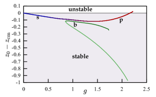
Figure 8: (Color online) Linear analysis concerning rotational stability for $\tilde{E_{B}}=0.01$. We show the (dimensionless) difference $z_{0}-z_{\text{c.m.}}$ between the center of hydrodynamic stress $z_{0}$ and the center of gravity $z_{\text{c.m.}}$ as a function of the dimensionless gravity strength $g$ for all three solution branches [(blue) pseudospherical, (red) pear-shaped, (green) buckled]. For $z_{0}-z_{\text{c.m.}}<0$, i.e., below the gray line, the shape is linearly stable against out-of-axis rotations. Only solutions with a very pronounced tether extrusion at high $g$ are unstable.

III.6 Accessible parameter space

With the shape diagram in Fig. 5 we have a complete overview of theoretically possible shapes and transitions between them in the plane of the two control parameters, the dimensionless bending rigidity $\tilde{E}_{B}$ or its inverse, the Föppl-von-Kármán number $\gamma_{\rm FvK}=1/\tilde{E}_{B}$, and the Bond number ${\rm Bo}=g$. There are three limitations, however, to the accessible parameter range.

First, our analysis is limited to the regime of low Reynolds numbers because we used the Stokes equation to describe the fluid flow. The Reynolds number for the sedimenting capsule is given by $\mathrm{Re}=v\rho R_{0}/\mu$. To leading order the sedimenting velocity is given by Stokes’ law $v=g_{0}\Delta\rho V/6\uppi\mu R_{0}$ resulting in $\mathrm{Re}=2g_{0}\Delta\rho\rho R_{0}^{3}/9\mu^{2}$. A criterion $\mathrm{Re}<1$ limits the accessible Bond numbers to $g<g_{\text{max, Re}}\sim 9\mu^{2}/2\rho R_{0}Y_{\rm 2D}$. For water as solvent we have $g_{\text{max, Re}}\sim 5\times 10^{-9}R_{0}^{-1}Y_{\rm 2D}^{-1}\,{\rm N}$. This can be easily increased by a factor of 100 in a more viscous solvent. For a capsule of size $R_{0}\sim 10{\rm\mu m}$ in water, the criterion $g<g_{\text{max, Re}}$ corresponds to a condition that the acceleration should remain smaller than 5000 times the standard gravity.

Second, the sedimenting force is very small for gravitation; it is much larger for a centrifuge but also modern ultracentrifuges are limited to accelerations about $10^{6}$ times the standard gravity Planken and Cölfen (2010). With a typical density difference of $\Delta\rho=10^{2}\,\mathrm{kg}/\mathrm{m^{3}}$ ($10\%$ of the density of water) we find that the Bond number is limited in available centrifuges to $g<g_{\text{max, cf}}\sim 10^{9}R_{0}^{2}Y_{\rm 2D}^{-1}\,\mathrm{N}/\mathrm{m}^{3}$.

Both of these constraints give an upper bound for the accessible Bond number range. The constraints are size dependent, however: For small capsule sizes $R_{0}\lesssim 1\,\mathrm{\mu m}$, for example, for viruses, the centrifuge constraint is more restrictive, whereas for larger capsule sizes $R_{0}\gtrsim 1\,\mathrm{\mu m}$, the low-Reynolds-number constraint is more restrictive. The latter case is typical for all synthetic capsules, red blood cells, or artificial cells consisting of a lipid bilayer and a filamentous cortex, which all have capsule sizes in the range $R_{0}\gtrsim 10~{}\text{to}~{}1000\mathrm{\mu m}$.

Third, it is not possible to realize arbitrarily large dimensionless bending rigidities $\tilde{E}_{B}=E_{B}/Y_{\rm 2D}R_{0}^{2}$ or small Föppl-von-Kármán numbers in experimentally available capsules. For isotropic elastic shell materials the relative shell thickness determines this parameter, $\tilde{E}_{B}\sim(H/R_{0})^{2}$, see Eq. (19), and values $\tilde{E}_{B}\gtrsim 0.01$ are difficult to realize with synthetic capsules. Viruses also follow this law (with a shell thickness $H\sim 2{\rm nm}$), resulting in Föppl-von-Kármán numbers $\gamma_{\rm FvK}\gtrsim 60$ or $\tilde{E}_{B}\lesssim 0.02$ with $\tilde{E}_{B}$ decreasing with increasing virus size Lidmar et al. (2003); small viruses with $R_{0}\sim 15{\rm nm}$ realize the largest values of $\tilde{E}_{B}$.

Red blood cells also have similar values of $\tilde{E}_{B}$ although they are elastically strongly anisotropic because they consist of a lipid bilayer and a spectrin cytoskeleton. The liquid lipid bilayer dominates the bending modulus $E_{B}\sim 50k_{B}T$, whereas the shear modulus is determined by the filamentous spectrin cortex or skeleton. Filamentous networks typically have low shear moduli, for example $G_{\rm 2D}\sim 10^{-6}{\rm N/m}$ for the spectrin skeleton of a red blood cell Lenormand et al. (2001). Using $Y_{\rm 2D}\sim 4G_{\rm 2D}$ for the red blood cell, because the lipid bilayer has a much higher area expansion modules $K_{\rm 2D}\sim 0.3{\rm N/m}$, we obtain $\tilde{E}_{B}\sim 0.005$ for a size $R_{0}\sim 3{\rm\mu m}$. Larger values of $\tilde{E}_{B}$ could be realized in artificial cells consisting of a lipid bilayer and a cortex from filamentous proteins for low filament densities in the cortex. These estimates of $\tilde{E}_{B}$ for red blood cells or artificial cells might, however, be misleading because the relevant elastic modulus in the elastic energy (18) is actually $Y_{\rm 2D}/(1-\nu^{2})$ rather than $Y_{\rm 2D}$, which is used in the standard definition of the Föppl-von-Kármán number and $\tilde{E}_{B}$, see Eq. (24). Because of their lipid bilayer, red blood cells or artificial cells are in the unstretchable limit $K_{\rm 2D}\gg G_{\rm 2D}$, where $\nu$ approaches unity, and we obtain $Y_{\rm 2D}/(1-\nu^{2})\approx K_{\rm 2D}$. Using this modulus in a definition of $\tilde{E}_{B}$ (i.e., in the non-dimensionalization) leads to much smaller values $\tilde{E}_{B}\sim 10^{-9}$.

The discontinuous sphere-pear transition happens beyond a critical point, $\tilde{E}_{B}>\tilde{E}_{B,c}\simeq 0.05$, see Fig. 5. Therefore, this peculiar transition is not accessible for typical synthetic capsules. To observe this transition an elastically very anisotropic capsule shell material with high bending and low stretching moduli would be needed. The transition into buckled shapes, however, should be well accessible with generic soft synthetic capsules.

The softness of the shell material is also important if high Bond numbers ${\rm Bo}\sim 1$ are to be realized in the shape diagram Fig. 5. In the presence of the above low-Reynolds-number constraint, very soft shell materials with a small two-dimensional Young modulus $Y_{\rm 2D}\lesssim 5\times 10^{-4}{\rm N/m}$ for a capsule of size $R_{0}\sim 10{\rm\mu m}$ are needed to reach such Bond numbers in water. Typical soft synthetic capsules such as OTS capsules have much larger moduli $Y_{\rm 2D}\sim 0.1{\rm N/m}$ Knoche et al. (2013). Red blood cells or artificial cells with shear moduli governed by a soft filamentous network have small moduli $Y_{\rm 2D}\sim 10^{-6}{\rm N/m}$, which will allow us to reach high Bond numbers. Again, these estimates might be misleading because the relevant elastic modulus in the elastic energy is actually $Y_{\rm 2D}/(1-\nu^{2})$ rather than $Y_{\rm 2D}$. If this modulus is used in the nondimensionalization and the definition of the Bond number in Eq. (25), Bond numbers become much smaller because red blood cells or artificial cells are hardly stretchable.

IV Localized driving forces

There are other possible external driving forces and self-propulsion mechanisms Ebbens and Howse (2010); Degen (2014). One extreme case is a very localized external force. We study this case by employing a driving pressure that acts on a small patch on one apex (we used the criterion $s_{0}\leq 0.1$ or $L-s_{0}\leq 0.1$, respectively; even more localized pressures would have to be higher and, thus, require smaller integration steps). For a pushing force, i.e., a force that acts on the stern of the capsule, this gives rise to strongly indented shapes. They have a higher drag than a spherical shape such that the driving force has to be higher than in Stokes’ law $u\approx F/6\uppi$ (in dimensionless form) resulting in $F_{\text{drive}}>6\uppi u$, whereas for pulling forces (acting on the bow) the drag is lower as compared to a sphere.

We show force-velocity relations with some exemplary shapes for these two types of external driving forces in Fig. 9. As can be seen clearly seen in the force-velocity relations, there are no shape bifurcations for elastic capsules driven by localized forces.

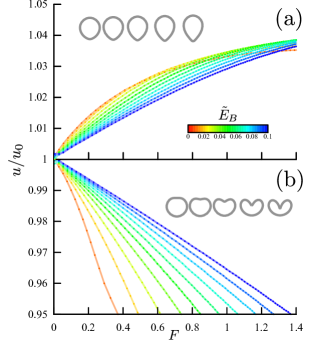
Figure 9: (Color online) Force-velocity relations for a capsule with fixed volume driven by (a) a localized pulling force and (b) a localized pushing force. The plots show the velocity relative to the (dimensionless) velocity $u_{0}=F/6\uppi$ of a hard sphere with same volume as a function of the (dimensionless) total external force. The insets show exemplary capsule shapes for $E_{B}=0.01$.

One way to apply a localized force experimentally is to attach beads to the capsule that can be manipulated via optical tweezers, as it has been done (for pulling and pushing types of forces) with giant vesicles in Ref. 48.

V Discussion and Conclusion

We introduced a new iterative solution scheme to find stationary axisymmetric shapes and velocity of a deformable elastic capsule driven through a viscous fluid by an external force at low Reynolds numbers. We focused on homogeneous body forces, i.e., sedimenting capsules in gravitation or in a centrifuge, but also demonstrated that other force distributions, such as localized forces, can be studied.

The iterative method is sufficiently accurate and fast to identify all branches of different shapes and to resolve dynamic shape transitions. We find a rich dynamic bifurcation behavior for sedimenting elastic capsules, even at fixed volume, see Fig. 5 with three types of possible axisymmetric stationary shapes: a pseudospherical state, a pear-shaped state, and buckled shapes. The capsule can undergo shape transformations as a function of two dimensionless parameters. The elastic properties are characterized by a dimensionless bending rigidity $\tilde{E}_{B}$ [the inverse Föppl-von-Kármán number, see Eq. (24)], and the driving force is characterized by the dimensionless Bond number [see Eq. (25)].

The transition between pseudospherical and pear shape is a discontinuous transition with shape coexistence and hysteresis for large bending rigidity or large Bond number. The corresponding transition line terminates, however, in a critical point if the bending rigidity is lowered, a phenomenon which is unknown from discontinuous static buckling transitions. Parameter estimates show that this transition cannot be observed with standard synthetic capsules because it requires a rather large bending rigidity or low Föppl-von-Kármán number, which cannot be realized for thin ($H/R_{0}<0.1$) shells of an isotropic elastic material. Observation of this discontinuous transition requires a material, which combines high bending rigidity while it remains highly stretchable.

We find an additional bifurcation into a pair of buckled shapes at small bending rigidities upon increasing the gravitational force. This bifurcation should be experimentally accessible with synthetic capsules in a centrifuge. The bifurcations are caused by hydrodynamic stretching, which increases a compressive hydrostatic pressure at the upper apex and leads to buckling-like transitions.

All shape bifurcations can be resolved in the force-velocity relation of sedimenting capsules, where up to three capsule shapes with different velocities can occur for the same gravitational driving force, see Fig. 6. In an experiment, these shapes are selected depending on the initial conditions. We also confirmed the stability of all axisymmetric shapes with respect to rotation around an axis perpendicular to the axis of symmetry, see Fig. 8. We find more stationary buckled shapes if we consider sedimenting capsules where we vary the volume by changing the pressure as it is explained in more detail in Appendix E. These additional shapes are higher order buckled shapes with more indentations.

It is instructive to discuss our results in comparison with sedimenting vesicles Boedec et al. (2011, 2012, 2013) and sedimenting red blood cells Peltomäki and Gompper (2013). Vesicles are bounded by a two-dimensional fluid lipid bilayer rather than a two-dimensional solid membrane or shell and are virtually unstretchable, i.e., they have a fixed area. Therefore, shape transitions from a spherical shape with the minimal area for given volume require excess area. For the sedimenting capsules this additional area is generated by hydrodynamic stretching. For vesicles, excess area can be “hidden” in thermal fluctuations. A spherical vesicle without such excess area cannot undergo any shape transitions during sedimentation. The pear shape for elastic capsules at high Bond numbers is similar to the “tether” formation by sedimenting vesicles Boedec et al. (2013). However, there are two important differences. First, the stretching energy of capsules penalizes deformations from the resting shape (whereas vesicles have a liquid surface that allows any shape with the correct area), which leads to less extreme and pronounced tethers. Moreover, cylindrical tethers are an actual equilibrium shape of a membrane under tension, which can coexist with a spherical vesicle Lipowsky et al. (2005). This is not the case for an elastic capsule. Secondly, we do not find a bulge or “droplet” forming at the upper end, by which we mean an increase in the width of the extrusion near the end of the tether. This is rooted in the different bending energies: Using a Helfrich bending energy that is quadratic in the mean curvature $w_{B}\sim(\kappa_{s}+\kappa_{\varphi})^{2}$, the negative meridional curvature ($\kappa_{s}<0$) needed to form a drop at the end of the tether is energetically favorable, whereas it is not with the Hookean bending energy (18) we employ. Moreover, elastic capsules cannot develop shapes with circulating surface flows because of their solid membrane. Therefore, there is no analog of the banana shape with surface flows that has been found in Refs. 23; 24 for vesicles.

Also sedimenting red blood cells exhibits different shapes; in MPCD simulations transitions between tear drop shapes, parachute (or cup-shaped) blood cells and fin-tailed shapes Peltomäki and Gompper (2013) have been found. Red blood cells have a non-spherical discocyte rest shape, which already provides some excess area as compared to the minimal area of a sphere. Therefore, stretching is not essential for dynamic shape transitions. The initial discocyte shape of red blood cells also gives rise to a strong tendency to tilt, which is absent for our initially spherical capsules. The parachute shape also tilts by almost $90^{\circ}$ during transformation into a tear drop Peltomäki and Gompper (2013). Interestingly, all transitions observed in Ref. 30 did not show any signatures in the force-velocity relation or the bending or shear energies. For spherical capsules we find clear signatures of all transitions in the force-velocity relation in Fig. 6. It remains to be clarified in future work whether the MPCD technique is not accurate enough or exhibits too many fluctuations to resolve these signatures or whether the dynamic transitions of sedimenting red blood cells qualitatively differ, for example, because tilt plays such a prominent role.

Finally, we studied capsules driven by localized forces, such as a pushing or pulling point-like force. For such localized driving forces, we always find shapes to transform smoothly without any shape bifurcations, see Fig. 9.

We plan to extend our iterative method to actively swimming capsules in future work Degen (2014). One possible swimming mechanism, for example in squirmer type swimmer models Blake (1971), is a finite velocity field at the capsule surface in its resting frame. Our solution technique using single-layer potentials remains still applicable as long as there is no net velocity normal to the surface (which indicates a fluid source or sink within the capsule and is, thus, not relevant).

Appendix A Single-layer potential solution of the Stokes equation in an axisymmetric domain

To make the paper self-contained, we give the analytical expressions for the elements of the matrix kernel $\mathsf{M}$ that relates the forces and the velocities on the surface of the capsule via

$$u_{\alpha}^{\infty}=-\frac{1}{8\uppi\mu}\int_{C}\mathrm{d}s(\mathbf{x})\mathsf{M}_{\alpha\beta}(\mathbf{y},\mathbf{x})f_{\beta}(\mathbf{x})~{}~{}(\mbox{for}~{}\mathbf{y}\in\partial B),$$ (28)

see Eq. (6). The derivation of this matrix kernel is briefly outlined in the main text and can also be found in Ref. 8.

As we are working in cylindrical coordinates $(r,z,\varphi)$ and the problem is axisymmetric, the matrix has four elements ($\alpha,\beta=r,z$) which can be explicitly written as

$$\mathsf{M}_{zz}(\mathbf{y},\mathbf{x}) =2k\sqrt{\frac{r_{x}}{r_{y}}}\left(F+\hat{z}^{2}E\right)$$ (29)

$$\mathsf{M}_{zr}(\mathbf{y},\mathbf{x}) =\frac{k\hat{z}}{\sqrt{r_{x}r_{y}}}\left(F-(r_{y}^{2}-r_{x}^{2}+\hat{z}^{2})E\right)$$ (30)

$$\mathsf{M}_{rz}(\mathbf{y},\mathbf{x}) =-k\frac{\hat{z}}{r_{y}}\sqrt{\frac{r_{x}}{r_{y}}}\left(F+(r_{y}^{2}-r_{x}^{2}-\hat{z}^{2})E\right)$$ (31)

$$\mathsf{M}_{rr}(\mathbf{y},\mathbf{x}) =\frac{k}{r_{x}r_{y}}\sqrt{\frac{r_{x}}{r_{y}}}\left[(r_{y}^{2}+r_{x}^{2}+2\hat{z}^{2})F\right.$$

$$\left.-(2\hat{z}^{4}+3\hat{z}^{2}(r_{y}^{2}+r_{y}^{2})+(r_{y}^{2}-r_{x}^{2})^{2})E\right]$$ (32)

using the abbreviations

$$\hat{z} \equiv z_{x}-z_{y}$$ (33)

$$k^{2} \equiv\frac{4r_{x}r_{y}}{\hat{z}^{2}+(r_{x}+r_{y})^{2}}$$ (34)

$$E \equiv\frac{E(k)}{\hat{z}^{2}+(r_{x}-r_{y})^{2}}$$ (35)

$$F \equiv K(k)$$ (36)

and the complete elliptic integrals of the first and second kinds Abramowitz and Stegun (1972),

$$K(k) =\int_{0}^{\uppi/2}\frac{\mathrm{d}\!x}{\sqrt{1-k^{2}\cos^{2}x}}$$ (37)

$$E(k) =\int_{0}^{\uppi/2}\mathrm{d}\!x\,\sqrt{1-k^{2}\cos^{2}x}$$ (38)

For the numerical computation of $\mathsf{M}$ elliptic integrals of the first and second kind we use polynomial approximants as given in Ref. 51.

Appendix B Validation of numerical method

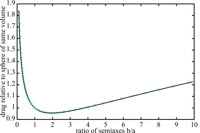
Figure 10: (Color online) Perrin factor $\Xi$, i.e., drag force onto a spheroid in a viscous fluid relative to that onto a sphere of same volume moving with the same velocity as a function of the ratio of the spheroid semiaxes $\xi=b/a$. The theoretical result (43) due to Perrin is shown as a solid (black) line and our numerical data as (green) crosses. The relative difference is less than $1/1000$ for all values, which validates our numerical approach.

We validate our algorithm and, in particular, our numerical treatment of singularities occurring in the boundary integral approach in Eq. (6) by comparison with exact analytical results for the Perrin factors for the total drag of a spheroid with semiaxes $a$ in radial and $b$ in axial direction Happel and Brenner (1983); Perrin (1936). A spheroid is an ellipsoid with two degenerate semiaxes $a$ in radial direction, i.e., it can be parametrized by

$$\mathbf{r} =\left(\begin{array}[]{c}a\cos\theta\sin\varphi\\ a\sin\theta\sin\varphi\\ b\cos\theta\end{array}\right)$$ (42)

with the polar angle $0\leq\varphi\leq 2\uppi$ and the parametric latitude $0\leq\theta\leq\uppi$.

The Perrin factor $\Xi$ is the ratio of the total drag force onto a spheroid with semiaxes ratio $\xi=b/a$ (for translation along the axial $a$ direction) and the drag of a sphere of the same volume moving with the same velocity. $\Xi$ is known analytically (from calculating the stream function in ellipsoidal coordinates) Perrin (1936),

$$\Xi =\begin{cases}\frac{\xi^{-\frac{1}{3}}}{\frac{3}{4}\sqrt{\xi_{p}^{2}-1}(-\xi_{p}+(\xi_{p}^{2}+1)\operatorname{artanh}(\xi_{p}^{-1}))}&\mbox{for}~{}\xi\geq 1\\ \frac{\xi^{-\frac{1}{3}}}{\frac{3}{4}\sqrt{\xi_{o}^{2}+1}(\xi_{o}-(\xi_{o}^{2}-1)\operatorname{atan}(\xi_{o}^{-1})}&\mbox{for}~{}\xi<1\end{cases}$$ (43)

with

$$\xi_{p} \equiv\sqrt{1-\xi^{-2}}^{-1}$$ (44)

$$\xi_{o} \equiv\sqrt{\xi^{-2}-1}^{-1},$$ (45)

for both prolate ($\xi\geq 1$) and oblate ($\xi\leq 1$) spheroids. We compare our numerical results to this analytical expression in Fig. 10 and find excellent agreement.

Appendix C First Integral of the shape equations

Inspired from the known first integral in the static problem (cf. Eqs. (17) and (22) in Ref. 37) we make the following ansatz for a first integral of the shape equations:

$$U(s) =2\uppi r\left(q\cos\psi+\tau_{s}\sin\psi\right)+X=\text{const.}$$ (46)

We are also assuming that the pressure $p$ and the shear pressure $p_{s}$ can be written as functions solely dependent on the arc length $s$. The calculation is rather straightforward: We differentiate using the shape equations (11) and the geometric relations (12) and get

$$0 =U^{\prime}(s)$$

$$=2\uppi q\cos^{2}\psi-2\uppi r\kappa_{s}q\sin\psi$$

$$~{}+2\uppi r\cos\psi\left((-\kappa_{s}\tau_{s}-\kappa_{\varphi}\tau_{\varphi}-\cos\psi\frac{q}{r}+p\right)$$

$$~{}+2\uppi\tau_{s}\cos\psi\sin\psi+2\uppi r\kappa_{s}\tau_{s}\cos\psi$$

$$~{}+2\uppi r\sin\psi\left(\cos\psi\frac{\tau_{\varphi}-\tau_{s}}{r}+\kappa_{s}q+p_{s}\right)+X^{\prime}$$

$$=2\uppi rp\cos\psi+2\uppi rp_{s}\sin\psi+X^{\prime}=0$$ (47)

In the second-to-last step most terms cancel each other out. Thus, we find an ordinary differential equation for $X$, which we can integrate directly:

$$X^{\prime} =-2\uppi r(p\cos\psi+p_{s}\sin\psi)$$

$$X =-2\uppi\int_{0}^{s}\mathrm{d}x\,r(p\cos\psi+p_{s}\sin\psi)$$ (48)

Inspecting the behavior at $s=0$ we then deduce $U(s)=U(0)=0$ or

$$0 =2\uppi rq\cos\psi+2\uppi r\tau_{s}\sin\psi+X.$$ (49)

The first integral $U(s)=0$ is indeed a generalization of the static quantity, as we see by setting $p_{s}=0$, $p=\text{const}$, which gives

$$X =-2\uppi p\int_{0}^{s}\mathrm{d}x\,r\cos\psi=-\uppi pr^{2},$$ (50)

and, thus, Eq. (49) becomes equivalent to Eq. (17) in Ref. 37.

The first integral is related to the global axial force balance of the capsule, which can be seen by considering $s=L$, where the $U(s)=U(L)=0$ gives $X(L)=0$. The quantity $X$ contains the contribution to the net force in the $z$ direction and thus a shape with the desired features (namely $q=0$ at the apexes) must have $X(L)=0$ and, thus, be in global force balance in axial direction.

Appendix D Rotational stability

We want to study the change in the torque due to an infinitesimally small rotation $\mathsf{R}$ of the velocity and the gravitational force vector. Geometrically, this is equivalent to rotating the capsule. A change of the velocity boundary condition $\mathbf{u}_{0}\rightarrow\mathbf{u}_{0}^{\prime}=\mathsf{R}\mathbf{u}_{0}$ leads to new hydrodynamic surface forces $\mathbf{f}\rightarrow\mathbf{f}^{\prime}$. As we did not change the capsule we can employ the reciprocal theorem

$$\int\mathrm{d}A\,\mathbf{u}\cdot\mathbf{f}^{\prime}=\int\mathrm{d}A\,\mathbf{u}_{0}^{\prime}\cdot\mathbf{f}$$ (51)

and find $\mathbf{f}^{\prime}=(\mathsf{R}^{T})^{-1}\mathbf{f}=\mathsf{R}\mathbf{f}$. The new hydrodynamic torque is, thus,

$$\mathbf{T_{u}}^{\prime}=\int\mathrm{d}A\,\left(\mathbf{r}\times\left(\mathsf{R}\mathbf{f}\right)\right)=\mathsf{R}\int\mathrm{d}A\,\left(\left(\mathsf{R^{-1}}\mathbf{r}\right)\times\mathbf{f}\right)\text{.}$$ (52)

We limit ourselves to a linear analysis, that is, we perform an infinitesimal rotation around the $y$ axis by an angle $\mathrm{d}\alpha$, i.e., $\mathsf{R}^{\pm 1}=\mathsf{I}\pm\mathrm{d}\alpha\mathsf{J}_{y}$. Here $\mathsf{I}$ is the unit matrix ($I_{ij}=\delta_{ij}$) and $\mathsf{J}_{y}$ generates a rotation around the $y$ axis with $\left(J_{y}\right)_{ij}=\delta_{i3}\delta_{j1}-\delta_{i1}\delta_{j3}$. Then, to linear order in $\mathrm{d}\alpha$,

$$\mathbf{e}_{y}\cdot\mathbf{T_{u}}^{\prime}=-2\uppi\mathrm{d}\alpha\int\mathrm{d}s\,r\left(\frac{1}{2}rf_{r}+(z-z_{0})f_{z}\right)\text{.}$$ (53)

Here $z_{0}$ gives the pivot point of the rotation. Since we know that the centers of mass and hydrodynamic stress have to lie on the symmetry axis, studying rotations about points on this axis suffices. Likewise, we can calculate the gravitational contribution to the new torque, which is (again to linear order in $\mathrm{d}\alpha$)

$$\mathbf{e}_{y}\cdot\mathbf{T_{g}}^{\prime}=\uppi\mathrm{d}\alpha g\int\mathrm{d}s\,r^{2}(z-z_{0})\text{.}$$ (54)

Equating these two gives the pivot point of the marginally stable infinitesimal rotation, i.e., the center of hydrodynamic stress.

This argument does not account for a change of the capsule shape due to the altered stresses upon rotation, which means that a seemingly unstable capsule might be stabilized axially by a “wobbling” deformation leading to different hydrodynamic torques. In principle, this might also work the other way round (as for semiflexible cylindrical rods Manghi et al. (2006)), but we think it is less relevant here, because of the typically large radius of curvature at the lower apex.

Appendix E Pressure control

For volume control, we fixed $V_{0}=4\uppi/3$ to the volume of the spherical rest shape and only explored the two parameters $\tilde{E}_{B}$ and $g$. The pressure $p_{0}$ served as Lagrange parameter to achieve the fixed volume $V_{0}$. To get a better understanding of the variety of shapes that are in principle possible, we study capsules with volumes other than that of the reference shape by controlling and changing the Lagrange parameter $p_{0}$. Thus, the explorable parameter space now consists of three parameters $\tilde{E}_{B}$, $g$, and $p_{0}$. As for volume control, the sedimenting velocity $u$ is not a control parameter but determined from demanding a force free capsule.

With the additional pressure parameter $p_{0}$, we find more sedimenting shapes to be stable (with different volumes), in particular, more classes of buckled shapes. We tried to find solutions at $\tilde{E}_{B}=0.01$ for pressures $p_{0}\in[-0.95,0.95]$ and $g\in[0,1]$. As a consequence of the quadratic nature of the elastic law, see Eq. (18), there is no solution for a resting capsule ($g=0$) with $p_{0}>1$ Knoche and Kierfeld (2011). For a cleaner comparison of different parameter sets (in particular for comparison of differently elongated shapes) it is helpful to not use $p_{0}$ but the pressure at the center of mass, $p_{\text{eff}}=p_{0}-\langle z\rangle g$, as an actual control parameter because we use a coordinate system that fixes $z=0$ at the lower apex of the capsule.

The possibility to explore a range of volumes allows for a greater variety of shapes. In Fig. 11, we show the pressure-volume relation for stationary axisymmetric shapes with a velocity close to $u=0.07$ (which determines for each shape a certain gravity $g$). Solutions at lower velocities are typically easier to find, but very low velocities are rather atypical because one ultimately sees the variety of static solutions Knoche and Kierfeld (2011). Each type of stable shape gives one pressure-volume branch in Fig. 11. Apart from pseudospherical, pear-shaped and the pair of weakly and strongly buckled solutions, we find additional branches, which correspond to higher-order buckled shapes with three, four, or five indentations.

As for fixed volume, the main contribution to the shape is due to static pressure (differences). For the pseudospherical branch this can be seen by comparing the volume (in reduced units) with the known pressure-volume relation for a spherical capsule in the static ($g=0$) case

$$V_{\text{sphere}}(p) =\frac{4\uppi}{3}\left(\frac{2}{p}\left(1-\sqrt{1-p}\right)\right)^{3}\,\text{,}$$ (55)

which fits our data rather well.

The higher-order buckled shapes occur at small volumes or small effective pressure $p_{\text{eff}}$. We expect to find corresponding higher-order buckled shapes also under volume control if we prescribe a corresponding small volume $V_{0}\sim 1-2$. But also for higher prescribed volumes such as $V_{0}=4\uppi/3\simeq 4.19$, these shapes could become stable at very high $g$: Higher volumes require a larger pressure $p_{\text{eff}}$ and, thus, also higher deformation forces to induce buckling. Such higher deformation forces can be achieved at high $g$.

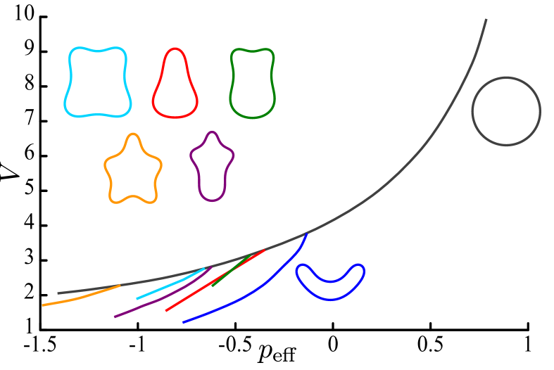
Figure 11: (Color online) Volume $V$ of the sedimenting elastic capsule as a function of the controlled pressure $p_{\text{eff}}$ at the center of mass at fixed bending rigidity $\tilde{E}_{B}=0.01$ and for shapes moving at a velocity $u\approx 0.07$. Each type of stable shape gives one pressure-volume branch. We identified the branches by the shape of the generatrices. We show one representative generatrix for each branch in the color of the branch. Please note that the generatrices are not drawn to scale. The pseudospherical branch is in good quantitative agreement with the static pressure-volume relation of Eq. (55).

References

- Barthès-Biesel (2011) D. Barthès-Biesel, Curr. Opin. Colloid Interface Sci. 16, 3 (2011).
- Fedosov et al. (2014) D. A. Fedosov, H. Noguchi, and G. Gompper, Biomech. Model. Mechanobiol. 13, 239 (2014).
- Freund (2014) J. B. Freund, Annu. Rev. Fluid Mech. 46, 67 (2014).
- Abreu et al. (2014) D. Abreu, M. Levant, V. Steinberg, and U. Seifert, Adv. Colloid Interface Sci. 208, 129 (2014).
- Huang et al. (2011) Z. Huang, M. Abkarian, and A. Viallat, New J. Phys. 13, 035026 (2011).
- Clift et al. (1978) R. Clift, J. Grace, and M. Weber, Bubbles, Drops, and Particles (Academic Press, New York, 1978).
- Stone (1994) H. A. Stone, Annu. Rev. Fluid Mech. 26, 65 (1994).
- Pozrikidis (1992) C. Pozrikidis, Boundary Integral and Singularity Methods for Linearized Viscous Flow (Cambridge University Press, Cambridge, 1992).
- Pozrikidis (2001) C. Pozrikidis, J. Comput. Phys. 169, 250 (2001).
- Meier (2000) W. Meier, Chem. Soc. Rev. 29, 295 (2000).
- Neubauer et al. (2014) M. P. Neubauer, M. Poehlmann, and A. Fery, Adv. Colloid Interface Sci. 207, 65 (2014).
- Pontani et al. (2009) L. L. Pontani, J. Van Der Gucht, G. Salbreux, J. Heuvingh, J. F. Joanny, and C. Sykes, Biophys. J. 96, 192 (2009).
- Tsai et al. (2011) F. C. Tsai, B. Stuhrmann, and G. H. Koenderink, Langmuir 27, 10061 (2011).
- Carvalho et al. (2013) K. Carvalho, F.-C. F. Tsai, E. Lees, R. Voituiriez, G. Koenderink, and C. Sykes, Proc. Natl. Acad. Sci. U.S.A. 110, 16456 (2013).
- Schäfer et al. (2013) E. Schäfer, T. T. Kliesch, and A. Janshoff, Langmuir 29, 10463 (2013).
- López-Montero et al. (2012) I. López-Montero, R. Rodríguez-García, and F. Monroy, J. Phys. Chem. Lett. 3, 1583 (2012).
- Saha et al. (2013) A. Saha, G. Mondal, A. Biswas, I. Chakraborty, B. Jana, and S. Ghosh, Chem. Commun. 49, 6119 (2013).
- Maeda et al. (2012) Y. T. Maeda, T. Nakadai, J. Shin, K. Uryu, V. Noireaux, and A. Libchaber, ACS Synth Biol. 1, 53 (2012).
- Vinogradova et al. (2006) O. I. Vinogradova, O. V. Lebedeva, and B.-S. Kim, Annu. Rev. Mater. Res. 36, 143 (2006).
- Lidmar et al. (2003) J. Lidmar, L. Mirny, and D. R. Nelson, Phys. Rev. E 68, 051910 (2003).
- Mukhopadhyay et al. (2002) R. Mukhopadhyay, G. Lim H W, and M. Wortis, Biophys. J. 82, 1756 (2002), arXiv:0108122 [cond-mat] .
- Lim H W et al. (2002) G. Lim H W, M. Wortis, and R. Mukhopadhyay, Proc. Natl. Acad. Sci. U.S.A. 99, 16766 (2002).
- Boedec et al. (2011) G. Boedec, M. Leonetti, and M. Jaeger, J. Comput. Phys. 230, 1020 (2011).
- Boedec et al. (2012) G. Boedec, M. Jaeger, and M. Leonetti, J. Fluid Mech. 690, 227 (2012).
- Boedec et al. (2013) G. Boedec, M. Jaeger, and M. Leonetti, Phys. Rev. E 88, 010702 (2013).
- Rey Suárez et al. (2013) I. Rey Suárez, C. Leidy, G. Téllez, G. Gay, and A. Gonzalez-Mancera, PLoS ONE 8, e68309 (2013).
- Corry and Meiselman (1978a) W. D. Corry and H. J. Meiselman, Biophys. J. 21, 19 (1978a).
- Corry and Meiselman (1978b) W. D. Corry and H. J. Meiselman, Blood 51, 693 (1978b).
- Hoffman and Inoué (2006) J. F. Hoffman and S. Inoué, Proc. Natl. Acad. Sci. U.S.A. 103, 2971 (2006).
- Peltomäki and Gompper (2013) M. Peltomäki and G. Gompper, Soft Matter 9, 8346 (2013).
- Noguchi and Gompper (2005) H. Noguchi and G. Gompper, Proc. Natl. Acad. Sci. U.S.A. 102, 14159 (2005).
- Fedosov et al. (2011) D. A. Fedosov, W. Pan, B. Caswell, G. Gompper, and G. E. Karniadakis, Proc. Natl. Acad. Sci. U.S.A. 108, 11772 (2011).
- Dupin et al. (2007) M. M. Dupin, I. Halliday, C. M. Care, L. Alboul, and L. L. Munn, Phys. Rev. E 75, 066707 (2007).
- Happel and Brenner (1983) J. Happel and H. Brenner, Low Reynolds Number Hydrodynamics: With Special Applications to Particulate Media, Vol. 1 (Springer, Berlin, 1983).
- Lauga and Powers (2009) E. Lauga and T. R. Powers, Rep. Prog. Phys. 72, 096601 (2009).
- Degen (2014) P. Degen, Curr. Opin. Colloid Interface Sci. 19, 611 (2014).
- Knoche and Kierfeld (2011) S. Knoche and J. Kierfeld, Phys. Rev. E 84, 046608 (2011).
- Knoche et al. (2013) S. Knoche, D. Vella, E. Aumaitre, P. Degen, H. Rehage, P. Cicuta, and J. Kierfeld, Langmuir 29, 12463 (2013).
- Libai and Simmonds (1998) A. Libai and J. Simmonds, The Nonlinear Theory of Elastic Shells (Cambridge University Press, Cambridge, 1998).
- Pozrikidis (2003) C. Pozrikidis, Modeling and Simulation of Capsules and Biological Cells (CRC Press, Boca Raton, FL, 2003).
- Landau and Lifshitz (1986) L. Landau and E. Lifshitz, Theory of Elasticity, Vol. 7 (Pergamon, New York, 1986).
- Pogorelov (1988) A. V. Pogorelov, Bendings of surfaces and stability of shells, Vol. 72 (American Mathematical Soc., Providence, 1988).
- Knoche and Kierfeld (2014) S. Knoche and J. Kierfeld, Soft Matter 10, 8358 (2014).
- Planken and Cölfen (2010) K. L. Planken and H. Cölfen, Nanoscale 2, 1849 (2010).
- ten Hagen et al. (2014) B. ten Hagen, F. Kümmel, R. Wittkowski, D. Takagi, H. Löwen, and C. Bechinger, Nat. Commun. 5, 4829 (2014).
- Lenormand et al. (2001) G. Lenormand, S. Hénon, a. Richert, J. Siméon, and F. Gallet, Biophys. J. 81, 43 (2001).
- Ebbens and Howse (2010) S. J. Ebbens and J. R. Howse, Soft Matter 6, 726 (2010).
- Dasgupta and Dimova (2014) R. Dasgupta and R. Dimova, J. Phys. D: Appl. Phys. 47, 282001 (2014).
- Lipowsky et al. (2005) R. Lipowsky, M. Brinkmann, R. Dimova, T. Franke, J. Kierfeld, and X. Zhang, J. Phys.: Condens. Matter 17, S537 (2005).
- Blake (1971) J. Blake, J. of Fluid Mech. 46, 199 (1971).
- Abramowitz and Stegun (1972) M. Abramowitz and I. A. Stegun, Handbook of Mathematical Functions: With Formulas, Graphs, and Mathematical Tables, 55 (Dover Publications, New York, 1972).
- Perrin (1936) F. Perrin, J. Phys. Radium 7, 1 (1936).
- Manghi et al. (2006) M. Manghi, X. Schlagberger, Y.-W. Kim, and R. R. Netz, Soft Matter 2, 653 (2006).