A unified heuristic and an annotated bibliography for a large class of earliness-tardiness scheduling problems
Abstract
This work proposes a unified heuristic algorithm for a large class of earliness-tardiness (E-T) scheduling problems. We consider single/parallel machine E-T problems that may or may not consider some additional features such as idle time, setup times and release dates. In addition, we also consider those problems whose objective is to minimize either the total (average) weighted completion time or the total (average) weighted flow time, which arise as particular cases when the due dates of all jobs are either set to zero or to their associated release dates, respectively. The developed local search based metaheuristic framework is quite simple, but at the same time relies on sophisticated procedures for efficiently performing local search according to the characteristics of the problem. We present efficient move evaluation approaches for some parallel machine problems that generalize the existing ones for single machine problems. The algorithm was tested in hundreds of instances of several E-T problems and particular cases. The results obtained show that our unified heuristic is capable of producing high quality solutions when compared to the best ones available in the literature that were obtained by specific methods. Moreover, we provide an extensive annotated bibliography on the problems related to those considered in this work, where we not only indicate the approach(es) used in each publication, but we also point out the characteristics of the problem(s) considered. Beyond that, we classify the existing methods in different categories so as to have a better idea of the popularity of each type of solution procedure.
Working Paper, UFPB – December 2016
1 Introduction
Scheduling problems have been widely studied in the literature over the past 50 years, receiving considerable attention from many scholars and practitioners around the world. Motivated by complex real-life problems faced by different types of companies, as well as by the challenge in solving them, a huge number of scheduling variants and solution procedures were proposed during this half-century period. Hence, it is safe to say that Scheduling is one of the most important subjects in the fields of Operations Research and Management Science.
A particular branch of the scheduling theory arises in the context of Just-In-Time (JIT) manufacturing systems. Problems of this branch of scheduling are generally referred to as earliness-tardiness (E-T) scheduling problems, where penalties are incurred if a job is completed before or after its due date. Moreover, they often include several additional features commonly found in the scheduling literature such as multiple machines (identical, uniform, unrelated), release dates, sequence-dependent setup times, among others.
Weighted E-T problems are usually -hard, since they include the single machine total weighted tardiness scheduling problem () as a particular case, which is known to be -hard (Lawler, 1977; Lenstra et al., 1977). Therefore, solving this type of problems to optimality is an extremely hard task. Nevertheless, there has been a continuous effort towards the development of efficient exact algorithms for this type of problems (Sourd and Kedad-Sidhoum, 2003; Sourd, 2005; Sourd and Kedad-Sidhoum, 2008; Tanaka and Fujikuma, 2008; Sourd, 2009; Tanaka et al., 2009; Pessoa et al., 2010; Tanaka and Fujikuma, 2012; Tanaka, 2012). In some particular situations, often involving a single machine environment without sequence-dependent setup times, they seem to be very effective, even solving instances with up to 300 jobs (Tanaka et al., 2009; Tanaka, 2012), but in most cases their application are still limited to small/medium-size instances. Heuristic algorithms are thus the natural alternative for trying to generate high quality feasible solutions within an acceptable computational time.
The large majority of heuristic algorithms proposed for scheduling problems were devised for a particular variant. While there are unified methods for polynomial problems (Leyvand et al., 2010) as well as polynomial time approximation schemes (Kumar et al., 2009; Epstein et al., 2013) and exact approaches (Chen and Powell, 1999; Tanaka and Fujikuma, 2008, 2012; Lin, 2013) for classes of -hard problems, we are not aware of general heuristics developed for similar purposes, as opposed, for example, to the field of vehicle routing, where there has been a trend in the development of efficient unified heuristics (Cordeau et al., 2001; Røpke and Pisinger, 2006; Pisinger and Røpke, 2007; Cordeau and Maischberger, 2012; Subramanian et al., 2013; Vidal et al., 2013, 2014; Derigs and Vogel, 2014).
Vehicle routing and single/parallel-machine scheduling problems have some similarities in the sense that in both problems one should determine the order in which the tasks (deliver goods to customers, processing a job in a machine, etc.) must be performed. However, there is a clear distinction between these two problems, especially when it comes to the objective function. In classical vehicle routing problems the objective is frequently to minimize the sum of the travel costs, whereas in scheduling problems the variety of objectives is more notable, ranging from minimizing the makespan or the total weighted completion time to minimizing the total weighted (earliness-)tardiness and so on. These differences on the objective functions have a direct influence, for instance, on the local search performance of a heuristic. In standard vehicle routing problems, a move can be often computed in constant time, while in scheduling problems more complex and specific procedures are generally required for evaluating the cost of a move. Moreover, while some aspects such as idle (waiting) times do not usually (directly) affect the objective function value in, for example, feasible solutions of vehicle routing problems with time windows, they may cause a considerable impact on the solution cost of E-T scheduling problems. These are just few examples of many of the issues that arise in scheduling problems that are generally relatively easier to handle in vehicle routing algorithms.
In addition, a heuristic that works well for scheduling problems without idle time may end up having a poor performance when applied to a variant in which idle time is allowed, mainly because in the latter one should solve a subproblem known as timing problem (Vidal et al., 2015b) that consists of determining the optimal start times of the jobs given a sequence. In fact, parts of a heuristic algorithm that were not designed to allow idle time should be substantially redesigned to address this point. Note that the opposite can also happen, that is, a heuristic designed to handle idle time may turn out to have a slow performance when considering instances without idle time.
In summary, it seems more challenging to devise a unified heuristic for standard scheduling problems than for vehicle routing problems, which may explain the lack of this kind of algorithms in the scheduling literature. Furthermore, we strongly believe that unified methods are extremely important in practice. For example, commercial packages must be designed to be both robust and general enough to efficiently deal with many real-life problems. Also, these type of methods can be a good source of reference if one intends to evaluate the performance of specially-tailored algorithms for some particular variants.
This work attempts to start filling the aforementioned gap by proposing a unified heuristic algorithm for single/parallel-machine scheduling problems. By “unified” we mean that several specific ingredients are put together into a single framework that is capable of efficiently solving a large class of distinct scheduling problems. However, due to the countless number of variants existing in the literature, we decided to focus our attention on a subset of them, in particular, E-T problems without preemption. We consider a class of problems that may or may not consider earliness penalties, sequence-dependent setup times, release dates, due dates and idle time, resulting in a broad range of variants that include other type of objectives such as minimizing the total weighted tardiness; total (average) weighted completion time; and total (average) weighted flow time.
The developed heuristic algorithm extends the one of Subramanian (2012); Subramanian et al. (2013) that was successfully applied to solve a class of vehicle routing problems. The conceptual idea of the proposed method is quite simple, however, in contrast to the original algorithm, some specific parts rely on sophisticated procedures (Ibaraki et al., 2005, 2008; Ergun and Orlin, 2006; Liao et al., 2012) for efficiently performing local search according to the characteristics of the problem. One particular contribution of this work is the development of efficient move evaluation approaches for a class of parallel machine problems. Such approaches generalize the ideas presented in Ergun and Orlin (2006) and Liao et al. (2012) for single machine total weighted tardiness problems. The algorithm was tested in benchmark instances of several E-T problems. The results obtained show that our unified heuristic is capable of producing high quality solutions when compared to the best ones available in the literature that were obtained by specific methods.
We also provide an extensive annotated bibliography on the problems related to those considered in this work, where we not only indicate the approach(es) used in each publication, but we also point out the characteristics of the problem(s) considered. In addition, we classify the heuristic and exact methods in different categories so as to have a better idea of the popularity of each type of solution procedure.
The remainder of this work is organized as follows. Section 3 presents an annotated bibliography on E-T works related to the class of problems considered in this research. Section 2 specifies the range of problems solve by our unified heuristic whose detailed description can be found in Section 4. Computational experiments are reported in Section 5. Finally, Section 6 contains the concluding remarks.
2 Problems considered
In this section we enumerate the class of E-T problems, including some particular cases, that our unified heuristic is capable of solving. We start by characterizing the general problem followed by a list of particular cases.
Let be a set of jobs to be scheduled on a set of unrelated parallel machines given by . For each job , let , , , and be its processing time in machine , due date, release date, earliness penalty weight and tardiness penalty weight, respectively. Also, let be the setup time required before starting to process job if is scheduled immediately after job in machine . The objective is to minimize , where and are the earliness and tardiness of a job , respectively, that depends on its completion time . Idle time is allowed to be inserted between two consecutive jobs. According to the notation suggested by Graham et al. (1979), this problem can be referred to as .
A large number of problems arise as a special case of the problem described above, including well-known single machine problems without sequence-dependent setup times such as , , , , that can be efficiently solved by the exact algorithm of Tanaka and Fujikuma (2012) for instances with up to 200 jobs (sometimes even 300 jobs as in the case of ). Note that the latter problem, which consists of minimizing the average weighted completion time, is a particular case of problem when all due dates are admitted to be zero, i.e., . Although the proposed heuristic is capable of dealing with these problems, its performance is simply not as good as some exact algorithms such as the one of Tanaka and Fujikuma (2012). In fact, it is really hard to devise heuristic algorithms with a superior or at least equivalent performance than the exact ones for these problems, even for large size instances. Our heuristic still finds high quality solutions for most of the existing instances, but not as fast as the state-of-the-art exact methods. For brevity, we decided not to report computational results for these problems.
Another type of objective function that arise as particular case of is when one aims at minimizing the average weighted flow time, which is given by . Note that by setting , we obtain .
Table 1 lists some of the main problems that appear as special case of problem and where our heuristic can be applied, including those mentioned above for the sake of completeness. Problems like do not appear in the table because we only considered -hard problems. We also do not explicitly include problems with unitary weights because they are simply particular cases of the weighted problems. For example, problem is well studied in the literature, but in principle any algorithm developed for problem can be used to solve the former one. In fact, some recent works on problem (Kirlik and Oğuz, 2012; Tanaka and Araki, 2013; Subramanian et al., 2014; Xu et al., 2014) also considered the version with unitary weights.
| Single machine | Identical machines | Uniform machines | Unrelated machines |
|---|---|---|---|
We did not perform computational experiments for all problems, not only for the reasons mentioned above, but also due to lack of publicly available instances. In addition, for some particular problems in which there are available instances, the authors who proposed them did not report lower/upper bounds.
3 An annotated bibliography for E-T problems related to those considered in this work
There is a vast literature on (E-)T scheduling. The first publications started to appear in the 1980s and they were surveyed by Baker and Scudder (1990). Another survey was later performed by Lauff and Werner (2004) for E-T problems in a multi-machine environment. Recently, Ratli et al. (2013) presented an overview on mathematical formulations and heuristics proposed for E-T problems but on a single machine environment. In these three works, the authors only reviewed problems with common due dates for all jobs. An entire book devoted to E-T scheduling was written by Józefowska (2007) where the author compiled the main models and algorithms for this class of problems, including those with common and individual due dates, respectively. The latter case is not only more general but also considered to be more challenging, since the first one has some properties that facilitates scheduling decisions. For example, it is known that idle time does not appear in the optimal solution of some variants where common due dates are considered, which makes the problem easier to be solved.
Moreover, problems with other characteristics such as learning effects, preemption, maintenance, deteriorating jobs, etc., are not considered in this section. We also do not consider approximation algorithms for problems that aim at minimizing either the total weighted completion time (in this case we refer the reader to the survey of Chekuri and Khanna (2004)) or the total flow time (see Kellerer et al. (1996); Leonardi and Raz (2007)). In addition, we only list the works published in the last 25 years. Finally, despite all our efforts in performing a complete enumeration of the large related literature, we cannot ensure that the annotated bibliography presented in this section include all the available relevant work.
3.1 Single machine environment
A considerable amount of the research involving (E-)T problems in the literature consider a single machine environment. Since there is a very large number of published works, it becomes rather impractical (and also it is beyond our goal) to provide a detailed description of each of them. Instead, we summarize, in chronological order, most of these works in Table LABEL:tab:SingleMachineWorks, where we specify the solution approach; the scheduling characteristics such as the existence of sequence-dependent setup-times (), release dates () and idle time (IT); and the type of objective considered by each method, namely (non-)weighted tardiness (), (non-)weighted earliness and tardiness (), (non-)weighted flow time () and (non-)weighted completion time ().
| Reference | Approach(es) | IT | ||||||
|---|---|---|---|---|---|---|---|---|
| Raman et al. (1989) | Constructive Heuristic | ✓ | ✓ | |||||
| Dyer and Wolsey (1990) | Formulations and valid inequalities | ✓ | ✓ | ✓ | ||||
| Potts and Van Wassenhove (1991) | SA, Constructive and randomized interchanging heuristics | ✓ | ✓ | |||||
| Yano and Kim (1991) | Heuristics, DP | ✓ | ✓ | |||||
| Belouadah et al. (1992) | B&B | ✓ | ✓ | ✓ | ||||
| Chu (1992a) | B&B | ✓ | ✓ | |||||
| Chu (1992b) | B&B | ✓ | ✓ | |||||
| Rubin and Ragatz (1995) | GA | ✓ | ✓ | |||||
| Della Croce (1995) | Local search, Lower bounds | ✓ | ✓ | ✓ | ✓ | |||
| Tan and Narasimhan (1997) | SA | ✓ | ✓ | |||||
| Li (1997) | B&B + LR, Heuristic | ✓ | ||||||
| Lee et al. (1997) | Constructive Heuristic | ✓ | ✓ | |||||
| Selim Akturk and Ozdemir (2000) | B&B | ✓ | ✓ | |||||
| França et al. (2001) | GA, MA | ✓ | ✓ | |||||
| Wan and Yen (2002) | TS | ✓ | ✓ | |||||
| Gagné et al. (2002) | ACO | ✓ | ✓ | |||||
| Congram et al. (2002) | Dynasearch, Iterated dynasearch, ILS | ✓ | ||||||
| Feldmann and Biskup (2003) | EA, SA, Threshold Accepting | ✓ | ||||||
| Sourd and Kedad-Sidhoum (2003) | B&B + LR | ✓ | ✓ | |||||
| Guo et al. (2004) | Experimental analysis with an approximation algorithm | ✓ | ✓ | |||||
| Grosso et al. (2004) | Dynasearch, Eliminations rules | ✓ | ||||||
| Sourd (2005) | Time-indexed formulation, B&B + LR, Multi-start heuristic | ✓ | ✓ | ✓ | ||||
| Gagné et al. (2005) | TS + VNS | ✓ | ✓ | |||||
| Cicirello and Smith (2005) | Heuristics | ✓ | ✓ | |||||
| Mason et al. (2005) | Moving block heuristic | ✓ | ✓ | |||||
| Ergun and Orlin (2006) | Fast neighborhood search | ✓ | ||||||
| Esteve et al. (2006) | Beam Search | ✓ | ✓ | ✓ | ||||
| Cicirello (2006) | GA | ✓ | ✓ | |||||
| Gupta and Smith (2006) | GRASP, PR, Problem Spaced-Based Local Search | ✓ | ✓ | |||||
| Hendel and Sourd (2006) | Efficient Local Search | ✓ | ✓ | |||||
| Sourd (2006) | Dynasearch | ✓ | ✓ | ✓ | ✓ | |||
| Bülbül et al. (2007) | Preemption based relaxation + Heuristic | ✓ | ✓ | ✓ | ||||
| M’Hallah (2007) | GA + Hill-Climbing + SA | ✓ | ||||||
| Liao and Juan (2007) | ACO | ✓ | ✓ | |||||
| Liao and Cheng (2007) | VNS + TS | ✓ | ||||||
| Lin and Ying (2007) | GA, SA, TS | ✓ | ✓ | |||||
| Tsai (2007) | GA | ✓ | ✓ | ✓ | ||||
| Pan and Shi (2008) | Hybrid approach: B&B + DP + CP | ✓ | ✓ | ✓ | ||||
| Tanaka and Fujikuma (2008) | SSDP | ✓ | ✓ | ✓ | ||||
| Anghinolfi and Paolucci (2008) | ACO | ✓ | ✓ | |||||
| Sourd and Kedad-Sidhoum (2008) | B&B + LR | ✓ | ✓ | ✓ | ||||
| Valente and Alves (2008) | Beam Search | ✓ | ✓ | |||||
| Bigras et al. (2008) | Formulations, B&B | ✓ | ✓ | |||||
| Anghinolfi and Paolucci (2009) | PSO | ✓ | ✓ | |||||
| Tasgetiren et al. (2009) | EA | ✓ | ✓ | |||||
| Arroyo et al. (2009) | ILS + GRASP | ✓ | ✓ | |||||
| Ying et al. (2009) | Iterated Greedy algorithm | ✓ | ✓ | |||||
| Sourd (2009) | B&B + LR | ✓ | ✓ | |||||
| Tanaka et al. (2009) | SSDP | ✓ | ✓ | |||||
| Geiger (2010) | Empirical Analysis | ✓ | ✓ | |||||
| Bozejko (2010) | Parallel SS | ✓ | ✓ | |||||
| Kedad-Sidhoum and Sourd (2010) | ILS, Fast Neighborhood Search | ✓ | ✓ | |||||
| Ronconi and Kawamura (2010) | B&B | ✓ | ||||||
| Yoon and Lee (2011) | Constructive heuristics | ✓ | ||||||
| Mandahawi et al. (2011) | ACO | ✓ | ✓ | |||||
| Kirlik and Oğuz (2012) | VNS | ✓ | ✓ | |||||
| Liao et al. (2012) | Fast neighborhood Search | ✓ | ✓ | |||||
| Sioud et al. (2012) | Hybrid GA | ✓ | ✓ | |||||
| Tanaka and Fujikuma (2012) | SSDP | ✓ | ✓ | ✓ | ✓ | ✓ | ||
| Tanaka (2012) | SSDP | ✓ | ✓ | ✓ | ||||
| Sioud et al. (2012) | GA + ACO | ✓ | ✓ | |||||
| Wan and Yuan (2013) | Proof of strongly -Hardness for problem | ✓ | ✓ | |||||
| Tanaka and Araki (2013) | SSDP | ✓ | ✓ | |||||
| Xu et al. (2013) | ILS | ✓ | ✓ | |||||
| Subramanian et al. (2014) | ILS | ✓ | ✓ | |||||
| Deng and Gu (2014) | ILS | ✓ | ✓ | |||||
| Guo and Tang (2015) | SS | ✓ | ✓ | |||||
| Subramanian and Farias (2015) | Efficient local search limitation strategy | ✓ | ✓ | |||||
From Table LABEL:tab:SingleMachineWorks, we can observe that the wide range of heuristic procedures for single machine problems proposed in the literature can be classified as follows:
- •
- •
-
•
Population based metaheuristics:
-
•
Local search based metaheuristics:
- •
-
•
Mathematical Programming based heuristics (Bülbül et al., 2007).
- •
As for the exact methods, they mostly consist of a partial combination between Dynamic Programming (DP), Lagrangian Relaxation (LR), Branch-and-Bound (B&B) and Mixed Integer Programming (MIP) formulations, and they can be categorized as follows:
3.2 Parallel machine environment
In this section we list the related works that considered parallel machines. Tables LABEL:tab:IdenticalParallelMachineWorks, LABEL:tab:UniformParallelMachineWorks and LABEL:tab:UnrelatedParallelMachineWorks summarize these works according to the environment, namely identical, uniform and unrelated parallel machine.
| Reference | Approach(es) | IT | ||||||
|---|---|---|---|---|---|---|---|---|
| Webster (1992) | Lower bounds | ✓ | ✓ | |||||
| Webster (1993) | Optimal priority rules for a special case of problem | ✓ | ✓ | |||||
| Webster (1995) | Lower bounds | ✓ | ✓ | |||||
| Belouadah and Potts (1994) | B&B + LR | ✓ | ||||||
| Lee and Pinedo (1997) | Preprocessing phase + Apparent tardiness cost with setups heuristic (ATCS) + SA | ✓ | ✓ | |||||
| Koulamas (1997) | Lower bounds, SA | ✓ | ||||||
| Azizoglu and Kirca (1998) | B&B | ✓ | ||||||
| Azizoglu and Kirca (1999) | B&B | ✓ | ||||||
| Chen and Powell (1999) | CG | ✓ | ||||||
| Radhakrishnan and Ventura (2000) | SA | ✓ | ✓ | |||||
| Eom et al. (2002) | EDD + ATCS + TS | ✓ | ✓ | |||||
| Yalaoui and Chu (2002) | B&B | ✓ | ||||||
| Sun and Wang (2003) | DP, Constructive heuristic | ✓ | ||||||
| Kim et al. (2006) | TS | ✓ | ✓ | ✓ | ✓ | |||
| Omar and Teo (2006) | MIP Formulation | ✓ | ✓ | ✓ | ||||
| Yalaoui and Chu (2006) | B&B | ✓ | ✓ | ✓ | ||||
| Shim and Kim (2007b) | B&B | ✓ | ||||||
| Kedad-Sidhoum et al. (2008) | Time-indexed formulation, LR, CG, Efficient local search | ✓ | ✓ | ✓ | ||||
| Feng and Lau (2008) | Squeaky Wheel Optimization (SWO) | ✓ | ✓ | ✓ | ||||
| Rios-Solis and Sourd (2008) | Exponential Neighborhood Search | ✓ | ||||||
| Pfund et al. (2008) | Apparent tardiness cost with setups and ready times (ATCSR) heuristic | ✓ | ✓ | ✓ | ✓ | |||
| Nessah et al. (2008) | B&B | ✓ | ✓ | ✓ | ||||
| Biskup et al. (2008) | Constructive Heuristic | ✓ | ||||||
| Rodrigues et al. (2008) | ILS | ✓ | ||||||
| Tanaka and Araki (2008) | B&B + LR | ✓ | ||||||
| Baptiste et al. (2008) | Lower Bounds | ✓ | ✓ | ✓ | ✓ | |||
| Mason et al. (2009) | Moving block heuristic | ✓ | ✓ | |||||
| Pessoa et al. (2010) | Time-indexed formulation, Branch-cut-and-price | ✓ | ||||||
| Jouglet and Savourey (2011) | B&B | ✓ | ✓ | ✓ | ||||
| M’Hallah and Al-Khamis (2012) | MIP, Hybrid heuristic (steepest descent + GA + SA) | ✓ | ✓ | |||||
| Della Croce et al. (2012) | ILS + Very Large Neighborhood Search | ✓ | ||||||
| Amorim et al. (2013) | Hybrid GA | ✓ | ||||||
| Amorim (2013) | GA, ILS, PR | ✓ | ||||||
| Schaller (2014) | TSs, GAs, B&B | ✓ | ✓ | |||||
| Xi et al. (2015) | Look-ahead constructive heuristic | ✓ | ✓ | ✓ | ✓ | |||
| Reference | Approach(es) | IT | ||||||
|---|---|---|---|---|---|---|---|---|
| Webster (1992) | Lower bounds | ✓ | ✓ | |||||
| Guinet (1995) | SA | ✓ | ||||||
| Azizoglu and Kirca (1998) | B&B | ✓ | ||||||
| Azizoglu and Kirca (1999) | B&B | ✓ | ||||||
| Chen and Powell (1999) | CG | ✓ | ||||||
| Sivrikaya-Şerifoğlu and Ulusoy (1999) | GA | ✓ | ✓ | ✓ | ✓ | |||
| Balakrishnan et al. (1999) | Mathematical formulation + Benders’ decomposition | ✓ | ✓ | ✓ | ||||
| Biskup and Feldmann (2001) | Benchmark instances | ✓ | ||||||
| Bilge et al. (2004) | TS | ✓ | ✓ | ✓ | ||||
| Anghinolfi and Paolucci (2007) | TS+SA+VNS | ✓ | ✓ | ✓ | ||||
| Armentano and de França Filho (2007) | GRASP | ✓ | ✓ | ✓ | ||||
| Raja et al. (2008) | SA + Fuzzy Logic | ✓ | ✓ | |||||
| Yousefi and Yusuff (2013) | Imperialist Competitive Algorithm | ✓ | ✓ | |||||
| Lin (2013) | Models / Formulations | ✓ | ||||||
| Li et al. (2014) | Agent-based algorithm + Lower Bounds | ✓ | ✓ | ✓ | ||||
| Reference | Approach(es) | IT | ||||||
|---|---|---|---|---|---|---|---|---|
| Webster (1992) | Lower bounds | ✓ | ✓ | |||||
| Zhu and Heady (2000) | MIP formulation | ✓ | ✓ | |||||
| Bank and Werner (2001) | Constructive + iterative heuristics, SA | ✓ | ✓ | ✓ | ||||
| Weng et al. (2001) | Constructive heuristics | ✓ | ✓ | |||||
| Liaw et al. (2003) | B&B | ✓ | ||||||
| Zhou et al. (2007) | ACO | ✓ | ||||||
| Shim and Kim (2007a) | B&B | ✓ | ||||||
| Logendran et al. (2007) | Six algorithms based on TS | ✓ | ✓ | ✓ | ||||
| Akyol and Bayhan (2008) | Neural network | ✓ | ✓ | |||||
| Li and lin Yang (2009) | Survey | ✓ | ✓ | ✓ | ||||
| Vallada and Ruiz (2012) | MIP formulation, GA | ✓ | ✓ | ✓ | ||||
| Lee et al. (2013) | TS | ✓ | ✓ | |||||
| Polyakovskiy and M’Hallah (2014) | Multi-Agent System Heuristic | ✓ | ✓ | |||||
| Nogueira et al. (2014) | GRASP + PR + ILS | ✓ | ✓ | ✓ | ||||
| Lin and Hsieh (2014) | Modified ATCSR and Electromagnetism-like Algorithm (EMA) | ✓ | ✓ | ✓ | ||||
| Bülbül and Şen (2016) | Preemptive relaxation + Benders’ decomposition | ✓ | ||||||
| Şen and Bülbül (2015) | Preemptive relaxation + Benders’ decomposition + solver SiPS/SiPSi (Tanaka et al., 2009) for obtaining upper bounds | ✓ | ✓ | ✓ | ✓ | |||
The heuristic approaches proposed for parallel machine problems can be classified as follows:
The exact methods developed for parallel machine problems can be classified as follows:
- •
- •
- •
- •
-
•
Preemption based relaxation (Bülbül and Şen, 2016).
4 The unified heuristic algorithm
The proposed unified heuristic, called UILS, is mostly based on ILS (Lourenço et al., 2002). This metaheuristic basically alternates between intensification (local search) and diversification (perturbation) procedures in order to escape from local optima. We modified the original ILS algorithm by allowing multiple restarts of the method. Previous works showed that this type of implementation, along with a Randomized Variable Neighborhood Descent (RVND) approach in the local search phase, yielded high quality results for different kinds of problems (Subramanian et al., 2010; Silva et al., 2012; Penna et al., 2013; Subramanian and Battarra, 2013; Martinelli et al., 2013; Subramanian et al., 2014; Vidal et al., 2015a; Subramanian and Farias, 2015), most of them in the field of routing, including the unified algorithms presented in Subramanian (2012); Subramanian et al. (2013).
Given the previous successful implementations of the multi-start ILS-RVND algorithm, we decided to extend this method to E-T scheduling problems. However, as pointed out in Section 1, several issues arise when dealing with scheduling problems that usually do not appear in vehicle routing problems. The main adaptation was in the local search phase where we implemented a tailored move evaluation approach according to the characteristics of the problem, such as the existence or not of earliness penalties, idle time, release dates and sequence-dependent setup times. This is one of the key aspects for the versatility and potential scalability of the proposed heuristic when facing problems with distinct features.
The multi-start heuristic starts by generating an initial solution using a very simple greedy randomized or a completely randomized insertion procedure. Next, a local search is performed using RVND, but with a specific move evaluation scheme that depends on the characteristics of the problem. On the one hand, when idles times are not considered, the choice of the move evaluation scheme to be used depends on the existence of setup times. On the other hand, when idle times are taken into account, the decision on the move evaluation scheme to be used depends on the presence of earliness penalties. Note that in this latter case, the existence of setup times does not affect such decision. Moreover, if the maximum number of consecutive perturbations without improvements () is not achieved (ILS stopping criterion), then the algorithm modifies the incumbent solution of the current multi-start iteration by applying a perturbation mechanism and then it restarts the local search procedure from that perturbed solution. Otherwise, the algorithm restarts from the beginning. If the maximum number of restarts () is achieved then the heuristic stops and returns the best solution found.
4.1 Initial Solutions
For problems involving multiple machines, the initial solutions are generated at random, whereas for single machine problems without release date the solutions are built either at random or following the earliest due date (EDD) method. When release dates are considered, the initial solutions are generated using the earliest release date (ERD) criterion. For the sake of diversification, EDD and ERD were implemented based on the greedy randomized approach of the constructive phase of GRASP (Feo and Resende, 1995).
It is worth mentioning that, based on preliminary experiments, the use of more sophisticated methods for building initial solutions do not significantly affect, on average, neither the quality of the final solution, nor the speed of convergence towards a local optimum. Hence, for simplicity, we decided to keep the constructive procedure as simple as possible.
4.2 Local Search
The local search is performed by a RVND procedure (Mladenović and Hansen, 1997; Subramanian, 2012), which consists of randomly choosing an unexplored neighborhood to proceed with the search every time another one fails to find an improved solution. Otherwise, all neighborhoods are allowed to be selected.
In what follows, we describe the neighborhood structures used in RVND, as well as the move evaluation procedures which can vary depending on the characteristics of the problem.
4.2.1 Neighborhood structures
With a view of better illustrating the neighborhood structures used in our algorithm we resort to a block representation, which is commonly adopted in the scheduling literature. Let be a sequence of jobs associated with a machine , with as a dummy job that is necessary for considering an eventual setup for processing the initial job of the sequence. A block consists of subsequence of consecutive jobs. An example involving 10 jobs divided into three blocks (, , ) is shown in Fig. 2.
The neighborhoods used in RVND are based on insertion and swap moves involving subsequences of jobs (blocks) and they are described next.
-
•
-block insertion intra-machine — consists of moving (reinserting) a block of size , starting from job , to the position after job in the same machine. A block () is moved forward (after ) when and , if ; and moved backward ( before ) when and , if , as depicted in Figs. 3 and 4, respectively.
Figure 3: -block insertion forward intra-machine Figure 4: -block insertion backward intra-machine -
•
-block swap intra-machine — consists of interchanging a block () of size , starting from job , with another one belonging to the same machine () of size , starting from job , as shown in Fig. 5.
Figure 5: -block Swap intra-machine -
•
-block insertion inter-machine — consists of removing a block () of size from a machine , starting from , and inserting it in machine at position , after block , as illustrated in Fig. 6.
Figure 6: -block insertion inter-machine -
•
-block swap inter-machine — consists of interchanging a block () of size of a machine , starting from job , with a block () of size of a machine that starts from job , as presented in Fig. 7.
Figure 7: -block Swap inter-machine
The size(s) of the block(s) in each type of neighborhood is an input parameter. Let , , and be the set of possible block sizes for the neighborhoods -block insert intra-machine, -block insert inter-machine, -block swap intra-machine and -block swap inter-machine, respectively. For example, if , we assume that there are 7 neighborhoods of the type -block insert intra-machine to be considered in the RVND procedure, each with a distinct value for . Similarly, if , then the RVND procedure will consider 6 neighborhoods of the type -block swap inter-machine, each of them with a different setting for .
The size of each individual neighborhood of any of the four types mentioned above is . For problems without idle time, a straightforward move evaluation can be performed in (Subramanian and Farias, 2015), leading to an overall complexity of for enumerating and examining all possible moves from that neighborhood. However, when there are no sequence-dependent setup times, the move evaluation can be performed in amortized time by extending the ideas presented in Ergun and Orlin (2006), yielding an overall complexity of . Otherwise, it is known that the move evaluation can still be performed in amortized time, but with an overall complexity of , by extending the approach proposed in Liao et al. (2012). Nevertheless, it appears that this approach is only worth to be implemented in practice for large sized instances/sequences.
For problems with idle time, one should solve the timing problem, i.e., determine the optimal start of the jobs associated with the solution under evaluation, which is usually solved by dynamic programming (Ibaraki et al., 2005), and the resulting overall complexity if often greater than the case without idle time. However, when earliness penalties are not considered and the need for idle time is due to the existence of release dates, the timing problem becomes trivial and one should only ensure that the job does not start before its release date. This can be done in time and therefore the overall complexity in this case is .
The next four sections present different ways of performing the move evaluation according to the characteristics of the problem.
4.2.2 Straightforward move evaluation for problems without idle time
Define and as the position associated with the first and last jobs of - block in the sequence, respectively, and define as the position associated with the last job of the preceding block in the sequence. Let be the completion time of the job in position . Alg. 1 shows how to compute the cost of block in ) steps.
The cost of a neighbor solution can be computed by simply summing up the cost of each block involved in the move. For example, when evaluating the cost of a move related to the -block swap intra-machine neighborhood, one can directly sum the costs of the blocks , , , , and (see Fig. 5) in this particular order. Note that the cost of a block depends on the completion time of the last job of the previous sequence, as illustrated in Alg. 1. In the worst case, the affected blocks may together contain all jobs of the instance, which imply in operations for computing the cost.
In order to speed up the process of computing the cost one can keep track of the cumulated cost up to a particular position of the sequence. Hence, define as a data structure that stores the cumulated cost up to the position of a sequence , more precisely:
where:
| (3) |
For example, the cost of block can be accessed in time by directly verifying the value of .
We remark that the straightforward way of computing the cost of a move described in this section is not new and we refer to Subramanian and Farias (2015) for a detailed description of the move evaluation using this type of approach. It is worthy of note that the same authors developed a local search limitation strategy, based on the setup variation due to a move, for problem that turned out to be very efficient in practice. They implemented a filtering mechanism that avoids unpromising moves to be evaluated. We believe that this idea can be extended for problems involving multiple machines and sequence-dependent setup times.
4.2.3 Move evaluation for problems without both idle time and sequence-dependent setup times
Ergun and Orlin (2006) presented ways of evaluating the moves of the neighborhoods -block insertion intra-machine, -block swap intra-machine and block reverse (a.k.a. twist) in amortized time for problem . In this work we extend their approaches for the neighborhoods described in Section 4.2.1 to solve problem (without idle time) and its particular cases, that is, all problems without sequence-dependent setup times and release dates shown in Table 1.
Before describing the move evaluation schemes for all neighborhoods, we will introduce some useful auxiliary functions and data structures.
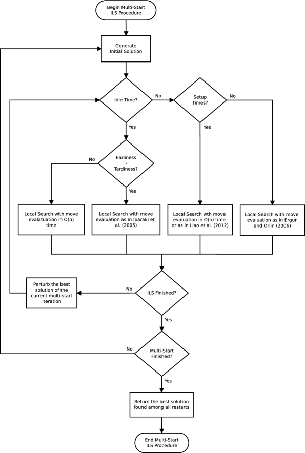
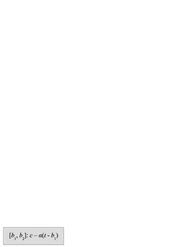
Let be a non-negative, convex and piecewise linear function that represents the penalty of start processing job in machine at time :
| (7) |
where is constant, positive and sufficiently large, used to penalize release date violation. For the ease of presentation we assume that . If this condition is not satisfied in practice, i.e. , then the functions above should be modified accordingly.
Each function is composed of three segments, where the transition points, a.k.a. breakpoints, are defined by , and . Release dates were considered for the sake of generality, but their existence typically enforce the presence of idle times. Since we are not considering idle times in this section, we can simply disregard one of the segments by setting , and the functions will remain valid, but with two segments each.
Now, for a given sequence , let be a piecewise linear function denoting the cost of a block composed of jobs sequenced in machine in this order and that job starts to be processed at time . Note that is the index of the last job assigned to machine . Each function , , can be determined by the following recursion:
To better clarify the meaning of functions and , consider the example given in Table 6, but disregarding the release dates and setup times.
Now assuming, for instance, that , we can write functions and as follows:
Fig. 8 illustrates a graphical representation of the piecewise linear functions.
Functions e can be stored in memory by means of linked lists, here denoted as L_j_k, where each element of the list is associated with one of the segments of the piecewise linear function. We use a data structure called seg to represent each segment of the function. Such data structure (see Fig. 9) stores the following piece of information:
-
•
: beginning of the segment’s interval;
-
•
: end of the segment’s interval;
-
•
c: value of the function at time ;
-
•
: slope of the segment.
In order to compute the cost of a block starting at time by means of functions using the information mentioned above, one needs to walk through the breakpoints of the corresponding function until the interval is reached and then compute the cost which is given by .
Finally, another important data structure is the so-called ProcessingList (Ergun and Orlin, 2006), which in our case is defined for all blocks of size from a given sequence . Each element of this list contains a pair of information, namely: pos and p, where the first stores the position of the first job of the block in the sequence, while the second stores the total processing time of the block in machine . The ProcessingList must be sorted in descending order according to the value of p. Alg. 2 shows how the ProcessingList is created.
Once the auxiliary functions and data structures were defined, it is now possible to show how to compute the cost of a sequence generated after applying one of the neighborhood operators.
For a given sequence , can have at most breakpoints. Since are piecewise linear functions, the complexity of obtaining the cost of a block starting at time is, in principle, , because in the worst case can be greater than the last breakpoint of the function. Hence, the complexity of evaluating a move would be . However, it is possible to evaluate a move of the neighborhoods in amortized time if the costs that depend on are precomputed following a given order.
Table 7 shows how to compute the cost of the modified solution in amortized time given that the costs that depend on are precomputed in . The first column identifies the blocks related to the move using the same convention adopted in Figures 3-7, while the remaining ones show how to compute the cost of each particular block depending on the neighborhood and machines involved in the move. Also, as shown in the referred figures, we can observe that the number of resulting blocks of a move varies from 4 to 6, according to the neighborhood. For example, a move of the neighborhood –block insertion inter considers blocks and on machine , and blocks and on machine . For a given solution, the indices and refer to the initial position of the blocks associated with the move (see Section 4.2.1 for more details). Hence, the cost of a neighbor solution can be computed by summing up the costs of the blocks involved in the move.
| Complexity of performing a single move evaluation in amortized time | ||||||
| -block insertion intra | (-)-block swap intra | -block insertion inter | (-)-block swap inter | |||
| Block | ||||||
| - | - | |||||
| - | - | |||||
| - | - | |||||
| - | - | |||||
| - | - | - | ||||
| - | - | - | - | - | ||
| Complexity of performing a single move evaluation in amortized / time | ||||||
| -block insertion intra | (-)-block swap intra | -block insertion inter | (-)-block swap inter | |||
| Block | ||||||
| - | - | |||||
| CompCostBlock | CompCostBlock | - | CompCostBlock | - | CompCostBlock | |
| - | - | |||||
| CompCostBlock | - | - | ||||
| - | - | CompCostBlock | - | |||
| - | - | - | - | - | ||
| Where: | ||||||
| ; ; ; ; | ||||||
| ; ; ; ; | ||||||
| ; ; ; . | ||||||
Nevertheless, since we adopted very small values for and , as will be shown in Section 5, we decided to implement the move evaluation schemes with complexity , where , as also shown in Table 7 rather than , which results in an overall complexity of , but in practice it seems to offer a more interesting scalability, even for large size instances. This happens because the preprocessing phase requires an additional overhead for dealing with blocks of size that in the end does not compensate the advantage of performing the move evaluations in steps.
The preprocessing consists of precomputing the costs of the blocks that depend on in a particular order. This enables the move evaluation procedure to access the cost of those blocks in constant time. For example, when performing the move evaluation of a neighbor solution after applying a move of the neighborhood -block insertion intra, one can compute the associated cost in constant time by means of the following expression: (see Table 7). The terms of this expression that depend on are precomputed in steps, as shown in (3), while the terms of this expression that depend on can be precomputed in steps, as explained next.
For example, in order to store all values of in steps, it is first necessary to sort the values of in ascending order. Note that this is possible to be achived by sorting the values of in ascending order, which can be done in by using a standard sorting procedure. Next, for every , it is now possible to compute the values of in steps, because this function has at most segments, which leads to an overall complexity of . A similar rationale can be applied to the other neighborhoods.
We will conclude this section by presenting alternative and simpler local search algorithms for the -block insertion neighborhoods that do not rely on the auxiliary data structures and functions mentioned above. The overall complexity of the search using such algorithms is and they are also based on the work of Ergun and Orlin (2006).
In the case of the intra-machine neighborhood, two similar but distinct procedures are required to move a block forward and backward in the sequence, respectively. Alg. 3 shows how the moves are evaluated when a block of size is removed and reinserted in a forward position in the sequence. It can be observed that moves are evaluated in steps (lines 9-12) by making use of the move evaluation performed immediately before the current one. The same rationale can be applied for moving blocks of size to a backward position in the sequence. Therefore, it can be verified that the overall complexity of Alg. 3 is .
Alg. 4 shows the pseudocode of the neighborhood -block insertion inter-machine. Note that when a block of size is removed from machine , one needs to compute the cost of the new sequence of only once and this can be done in steps as in Section 4.2.2. As for machine , where the block is going to be inserted in several positions, the cost of each modified sequence can be computed in using the same idea presented in Alg. 3 after computing the cost of inserting the block in the first position in also as in Section 4.2.2. Hence, the overall complexity of Alg. 4 is .
4.2.4 Move evaluation for problems with sequence-dependent setup times but without idle time
Liao et al. (2012) showed, for problem , that is possible to perform the move evaluations of the same neighborhoods considered by Ergun and Orlin (2006) in amortized time, but at the expense of preprocessing the required auxiliary data structures in operations. Their method is based on the one of the latter authors and it can be extended to solve problem and its particular cases (only those without idle time) by using the same rationale presented in Section 4.2.3.
The main difference between the approaches of Liao et al. (2012) and Ergun and Orlin (2006) is the preprocessing phase, where the sorting procedure should be called for each before computing the values of for each in the sequence, because now depends on the existing setup times, thus leading to a complexity of .
Nevertheless, this approach seems to be indicated for large scale instances, as suggested by the experiments performed in Liao et al. (2012). For small-medium scale instances the procedure described in Section 4.2.2 appears to be more suitable to address the problems with sequence-dependent setup times listed in Table 1.
4.2.5 Move evaluation for problems with idle time
Ibaraki et al. (2005) proposed an efficient approach for evaluating the moves during the local search when idle times are considered. In this case, the timing problem, which consists of determining the optimal start time of each job in the sequence, should also be solved when evaluating the cost of a solution. The authors first present a dynamic programming based algorithm to solve this problem and then they show how to integrate such method within the local search.
As in Ergun and Orlin (2006), the method of Ibaraki et al. (2005) relies on auxiliary data structures and functions. The idea is to determine functions that return the minimum penalty of the subsequences (blocks) when starting at a particular time , both forward and backward. The cost of the solution under evaluation is thus computed by using such information over the resulting sequence obtained after concatenating certain subsequences.
In Ibaraki et al. (2008) the authors suggested a balanced binary tree based implementation that allows for solving the timing problem in time, where denotes the total number of segments of the penalty function for the jobs sequenced in machine . As demonstrated by the authors, a move can be evaluated in amortized time, where is the largest among the machines involved. The necessary functions of each machine can be precomputed in steps. However, for simplicity, we used a linked list based implementation (Ibaraki et al., 2005), which yields an amortized complexity of where the necessary functions for each machine can be precomputed in steps.
4.3 Perturbation Mechanisms
The following three perturbation mechanisms were implemented:
-
•
()-block swap intra-machine: one ()-block swap intra-machine move is performed at random with and .
-
•
Multiple ()-insertion inter-machine: a job from a machine is moved to a machine , while a job from is moved to . The jobs, machines and positions to be inserted are all chosen at random and such procedure is repeated one, two or three consecutive times.
-
•
Multiple ()-block insertion inter-machine: this perturbation generalizes the previous one but in this case blocks of jobs of sizes and , respectively, are involved in the move with and .
The first mechanism is only applied for single machine problems, while the second and third are only applied for parallel machine problems and they are chosen at random.
5 Computational experiments
The UILS algorithm was coded in C++ and the experiments were executed in an Intel Core i7-2600 with 3.40 GHz and 16 GB of RAM running under Ubuntu Linux 12.04. Only a single thread was used in our testing. The proposed algorithm was executed 10 times for each instance in the final experiments. Furthermore, with a view of better comparing the runtime performance between UILS and other methods from the literature that used machines with a quite inferior hardware performance than ours, we have scaled the CPU time values reported in their work to our machine. This was done by means of approximation factors that were computed using the single thread rating values reported in https://www.cpubenchmark.net/.
Unfortunately, the vast majority of the problems listed in Table 1 does not have publicly available instances. Most authors usually generate the instances for a particular problem themselves but they seldom make them easily accessible for the research community. Table 8 lists some problems in which we are aware that there are instances available online. We executed the UILS algorithm only for those with results reported in the literature.
We remark that we do not present the results obtained by our algorithm for the publicly available instances of problems and , because those found by a similar and simplified version of this algorithm were already reported in Subramanian et al. (2014). UILS still finds slightly better results than the simplified algorithm, but for brevity we chose not report them here. We also do not report the results found for the publicly available instances of single machine problems without sequence-dependent setup times, in particular, , , , , , because they are well-solved by the highly sophisticated exact algorithms of Tanaka et al. (2009); Tanaka and Fujikuma (2012). UILS even finds the optimal solutions of such instances but not as fast as the exact methods. Moreover, we are not aware of any heuristic method whose performance is comparable to the exact ones for these problems.
| Problem | Instances | Related work | ||
| and | to | Tanaka and Araki (2008) | ||
| to | and | Rodrigues et al. (2008); Pessoa et al. (2010) | ||
| to | and | Amorim et al. (2013); Amorim (2013) | ||
| to | to | Şen and Bülbül (2015) | ||
| to | to | Şen and Bülbül (2015) | ||
| 1 Available at: https://sites.google.com/site/shunjitanaka/pmtt | ||||
| 2 Available at: http://algox.icomp.ufam.edu.br/index.php/benchmark-instances/weighted-tardiness-scheduling | ||||
| 3 Available at: http://algox.icomp.ufam.edu.br/index.php/benchmark-instances/weighted-earliness-tardiness-scheduling | ||||
| 4 Available at: http://people.sabanciuniv.edu/~bulbul/papers/Sen_Bulbul_Rm_TWT-TWET_source-data-results_IJOC_2015.rar | ||||
5.1 Parameter tuning
In this section we explain how we tuned the main parameters of UILS, that is, , , and the neighborhood sets , , and .
We start by describing how we selected the neighborhood sets. We used an incremental approach where we included one neighborhood at a time in ascending order of and , and then we evaluated the impact on the solution quality after such inclusion. More precisely, for every new neighborhood considered, we applied the RVND procedure over an initial solution and then we computed the value of the gap of the resulting local optimum with respect to the initial solution. Initially, only one neighborhood of a particular type was considered, namely 1-block insertion intra-machine, and then we kept increasing the set until no improvement was verified. In this case, we stopped adding the -block insertion intra-machine neighborhoods and started including -block swap intra-machine neighborhoods until no improvement was observed. Then we included the -block insertion inter-machine neighborhoods and, finally, the -block swap intra-machine neighborhoods.
We selected 24 challenging instances among those available for problem (without idle time) to determine the neighborhood sets. For each instance and for each combination of neighborhoods, we ran the RVND procedure 5 times over different initial solutions and we stored the average improvement obtained. Table 9 reports the average improvements obtained for each combination. Strikethrough entries correspond to those neighborhoods that have been disregarded due to lack of average improvement on the solution quality. The following sets were selected: , , and .
It is worth mentioning that for single machine problems we considered and as in Subramanian et al. (2014).
| Neighborhoods | Avg. Imp. |
| (%) | |
| 1-block insertion intra-machine | 64.22 |
| + 2-block insertion intra-machine | 64.33 |
| + 3-block insertion intra-machine | 63.33 |
| + (1.1)-swap intra-machine | 65.75 |
| + (1.2)-swap intra-machine | 65.63 |
| + 1-block insertion inter-machine | 67.50 |
| + 2-block insertion inter-machine | 68.01 |
| + 3-block insertion inter | 67.62 |
| + (1.1)-swap inter-machine | 68.04 |
| + (1.2)-swap inter-machine | 68.32 |
| + (1.3)-swap inter-machine | 69.02 |
| + (2.2)-swap inter-machine | 69.22 |
| + (2.3)-swap inter-machine | 69.47 |
| + (2.4)-swap inter-machine | 69.58 |
| + (3.3)-swap inter-machine | 69.63 |
| + (3.4)-swap inter-machine | 69.65 |
| + (4.4)-swap inter-machine | 69.79 |
| + (4.5)-swap inter-machine | 69.63 |
In order to tune the parameter we performed a series of experiments for the same 24 instances previously selected. We considered different values, namely, , , , and . We noticed that a single start of the method, i.e. , led to inconclusive results. Hence, we decided to adopt as in Subramanian et al. (2014) in order to better calibrate the value of . Table 10 show the results obtained with different values of where the gap reported for every instance is between the average solution of 5 runs and the best known solution (BKS). We also report the average time of the 5 runs, as well as the number of times BKS was found or improved.
| Instance | |||||||||||||||
| Gap | Time | #BKS | Gap | Time | #BKS | Gap | Time | #BKS | Gap | Time | #BKS | Gap | Time | #BKS | |
| (%) | (s) | (%) | (s) | (%) | (s) | (%) | (s) | (%) | (s) | ||||||
| wet100-10m-121 | 0.08 | 20.5 | 0 | 0.06 | 31.9 | 0 | 0.05 | 57.2 | 0 | 0.03 | 111.0 | 0 | 0.03 | 172.0 | 0 |
| wet100-10m-31 | 0.78 | 29.2 | 0 | 0.63 | 52.7 | 0 | 0.47 | 96.6 | 0 | 0.37 | 173.5 | 0 | 0.29 | 264.6 | 0 |
| wet100-10m-61 | 0.43 | 24.5 | 0 | 0.34 | 39.1 | 0 | 0.25 | 76.6 | 0 | 0.18 | 116.5 | 0 | 0.09 | 182.5 | 1 |
| wet100-2m-1 | 0.02 | 34.2 | 0 | 0.01 | 64.2 | 0 | 0.01 | 148.9 | 0 | 0.00 | 262.4 | 0 | 0.00 | 411.1 | 1 |
| wet100-2m-11 | 0.04 | 30.6 | 1 | 0.02 | 67.5 | 0 | 0.02 | 101.1 | 0 | 0.00 | 174.8 | 3 | 0.01 | 244.5 | 2 |
| wet100-2m-111 | 0.08 | 34.0 | 0 | 0.05 | 67.6 | 0 | 0.00 | 136.5 | 2 | 0.01 | 219.3 | 2 | 0.00 | 307.8 | 1 |
| wet100-2m-121 | 0.01 | 20.5 | 0 | 0.01 | 40.1 | 0 | 0.00 | 83.2 | 1 | 0.00 | 131.5 | 2 | 0.00 | 209.4 | 4 |
| wet100-2m-31 | 0.07 | 34.0 | 0 | 0.02 | 64.0 | 0 | 0.02 | 121.4 | 0 | 0.00 | 227.0 | 1 | 0.00 | 347.4 | 2 |
| wet100-2m-61 | 0.13 | 31.3 | 0 | 0.04 | 55.8 | 0 | 0.02 | 95.4 | 0 | 0.00 | 174.3 | 5 | 0.00 | 234.3 | 3 |
| wet100-2m-71 | 0.00 | 17.0 | 0 | 0.00 | 32.7 | 1 | 0.00 | 58.5 | 2 | 0.00 | 99.7 | 2 | 0.00 | 140.7 | 3 |
| wet100-2m-81 | 0.37 | 37.1 | 0 | 0.25 | 65.4 | 0 | 0.17 | 109.1 | 0 | 0.10 | 244.9 | 1 | 0.08 | 293.7 | 1 |
| wet100-2m-91 | 0.02 | 25.4 | 1 | 0.01 | 47.8 | 2 | 0.00 | 81.4 | 4 | 0.00 | 125.8 | 4 | 0.00 | 182.0 | 5 |
| wet100-4m-111 | 0.29 | 35.1 | 0 | 0.26 | 80.3 | 0 | 0.20 | 131.1 | 0 | 0.09 | 238.5 | 0 | 0.14 | 337.6 | 0 |
| wet100-4m-31 | 0.44 | 33.8 | 0 | 0.23 | 72.6 | 0 | 0.26 | 134.5 | 0 | 0.19 | 274.1 | 0 | 0.17 | 374.5 | 0 |
| wet100-4m-61 | 0.30 | 33.5 | 0 | 0.22 | 66.2 | 0 | 0.18 | 102.9 | 0 | 0.15 | 219.0 | 0 | 0.06 | 271.6 | 1 |
| wet100-4m-81 | 2.06 | 38.6 | 0 | 1.89 | 75.9 | 0 | 1.56 | 143.8 | 0 | 0.91 | 248.7 | 0 | 0.85 | 379.6 | 0 |
| wet150-2m-1 | 0.02 | 124.0 | 0 | 0.02 | 257.8 | 0 | 0.01 | 564.7 | 0 | 0.01 | 1044.1 | 0 | 0.00 | 1569.2 | 0 |
| wet200-2m-1 | 0.02 | 385.9 | 0 | 0.02 | 825.3 | 0 | 0.01 | 1725.8 | 0 | 0.01 | 3603.8 | 0 | 0.01 | 5201.9 | 0 |
| wet40-2m-1 | 0.02 | 1.4 | 0 | 0.00 | 2.5 | 3 | 0.00 | 5.8 | 5 | 0.00 | 9.1 | 5 | 0.00 | 11.8 | 5 |
| wet40-4m-1 | 0.24 | 1.5 | 0 | 0.10 | 3.1 | 1 | 0.02 | 5.6 | 3 | 0.02 | 11.0 | 3 | 0.00 | 14.2 | 5 |
| wet40-4m-111 | 0.01 | 1.3 | 4 | 0.00 | 2.8 | 5 | 0.00 | 4.3 | 5 | 0.00 | 7.6 | 5 | 0.00 | 11.4 | 5 |
| wet40-4m-121 | 0.00 | 0.9 | 5 | 0.00 | 1.6 | 5 | 0.00 | 2.6 | 5 | 0.00 | 4.5 | 5 | 0.00 | 6.2 | 5 |
| wet40-4m-91 | 0.03 | 1.1 | 4 | 0.00 | 1.8 | 5 | 0.00 | 3.4 | 5 | 0.00 | 6.7 | 5 | 0.00 | 9.3 | 5 |
| wet50-2m-1 | 0.02 | 3.2 | 0 | 0.02 | 5.4 | 0 | 0.01 | 10.8 | 0 | 0.00 | 19.4 | 1 | 0.00 | 28.9 | 0 |
| Avg. | 0.23 | 41.6 | – | 0.18 | 84.3 | – | 0.14 | 166.7 | – | 0.09 | 322.8 | – | 0.07 | 466.9 | – |
| Total | – | – | 15 | – | – | 22 | – | – | 32 | – | – | 44 | – | – | 49 |
The results illustrated in Table 10 suggest that and seem to be superior in terms of solution quality than the other settings, but not very different from each other. We decided to adopt because it seemed to provide an interesting compromise between solution quality and average CPU time.
We performed similar experiments considering and , but the increment in the CPU time due to more restarts do not seem to compensate the slight increase in the solution quality. Therefore, we chose to keep , but limiting the total execution time to seconds in order to avoid long runs for large instances.
While performing further experiments, we realized that the proposed algorithm performed quite slow for problems with idle time when adopting . This is because the local search phase is more expensive in terms of CPU time, as already explained. We thus performed a similar experiment as the one just described above, but for 10 selected instances of problem . In this case we only considered the following values for : , and . Furthermore, since UILS systematically found or improved the BKS, we decided to evaluate the gap with respect to the lower bound and also with respect to our best solution (OBS) so as to better appreciate the influence of the parameter. The results of these experiments are reported in Table 11. By following a similar criterion used in the previous case, we decided to adopt for problems with idle time.
| Instance | ||||||||||||
| GapLB | GapOBS | Time | #OBS | GapLB | GapOBS | Time | #OBS | GapLB | GapOBS | Time | #OBS | |
| (%) | (%) | (s) | (%) | (%) | (s) | (%) | (%) | (s) | ||||
| WET40_R2_25_100_021 | 1.87 | 0.01 | 18.3 | 4 | 1.86 | 0.00 | 31.7 | 5 | 1.86 | 0.00 | 59.5 | 5 |
| WET40_R2_25_100_101 | 0.00 | 0.00 | 5.8 | 5 | 0.00 | 0.00 | 10.2 | 5 | 0.00 | 0.00 | 18.7 | 5 |
| WET60_R2_25_100_021 | 1.25 | 0.07 | 131.2 | 1 | 1.18 | 0.00 | 245.3 | 5 | 1.19 | 0.02 | 391.3 | 4 |
| WET60_R2_25_100_101 | 0.08 | 0.00 | 33.3 | 5 | 0.08 | 0.00 | 60.4 | 5 | 0.08 | 0.00 | 102.9 | 5 |
| WET60_R3_25_100_021 | 0.05 | 0.04 | 102.7 | 3 | 0.01 | 0.00 | 204.2 | 4 | 0.01 | 0.00 | 363.1 | 5 |
| WET60_R3_25_100_101 | 0.01 | 0.00 | 31.6 | 5 | 0.01 | 0.00 | 53.5 | 5 | 0.01 | 0.00 | 95.6 | 5 |
| WET80_R2_25_100_021 | 1.24 | 0.13 | 547.5 | 1 | 1.14 | 0.03 | 951.4 | 1 | 1.12 | 0.01 | 1534.3 | 3 |
| WET80_R2_25_100_101 | 0.02 | 0.00 | 119.5 | 5 | 0.02 | 0.00 | 233.1 | 5 | 0.02 | 0.00 | 390.6 | 5 |
| WET90_R3_25_100_021 | 1.43 | 0.39 | 656.8 | 0 | 1.09 | 0.05 | 1307.7 | 1 | 1.09 | 0.05 | 2010.7 | 2 |
| WET90_R3_25_100_101 | 0.16 | 0.00 | 162.4 | 5 | 0.16 | 0.00 | 253.3 | 5 | 0.16 | 0.00 | 409.0 | 5 |
| Avg. | 0.61 | 0.06 | 180.9 | – | 0.56 | 0.01 | 335.1 | – | 0.55 | 0.01 | 537.6 | – |
| Total | – | – | – | 34 | – | – | – | 41 | – | – | – | 44 |
5.2 Results for problem
The optimal solutions of all 2250 instances available for problem were found by the exact method of Tanaka and Araki (2008). The UILS algorithm was capable of finding such optima in at least 9 of the 10 runs and the average computational time was smaller than one second, as can be observed in Table 12.
| Instance | #Inst | Tanaka and Araki (2008) | UILS | ||||
| group | Time1 | Gap | Gap | Time | #Best | #Opt | |
| (s) | (%) | (%) | (s) | ||||
| N20_M2 | 125 | 0.2 | 0.00 | 0.00 | 0.3 | 1250 | 125 |
| N20_M3 | 125 | 0.1 | 0.00 | 0.00 | 0.3 | 1250 | 125 |
| N20_M4 | 125 | 0.1 | 0.00 | 0.00 | 0.3 | 1250 | 125 |
| N20_M5 | 125 | 0.00 | 0.00 | 0.3 | 1250 | 125 | |
| N20_M6 | 125 | 0.00 | 0.00 | 0.3 | 1250 | 125 | |
| N20_M7 | 125 | 0.00 | 0.00 | 0.3 | 1250 | 125 | |
| N20_M8 | 125 | 0.00 | 0.00 | 0.3 | 1244 | 125 | |
| N20_M9 | 125 | 0.00 | 0.00 | 0.2 | 1247 | 125 | |
| N20_M10 | 125 | 0.00 | 0.00 | 0.2 | 1248 | 125 | |
| N25_M2 | 125 | 0.5 | 0.00 | 0.00 | 0.6 | 1250 | 125 |
| N25_M3 | 125 | 6.3 | 0.00 | 0.00 | 0.6 | 1247 | 125 |
| N25_M4 | 125 | 15.5 | 0.00 | 0.00 | 0.6 | 1248 | 125 |
| N25_M5 | 125 | 4.7 | 0.00 | 0.00 | 0.6 | 1244 | 125 |
| N25_M6 | 125 | 0.1 | 0.00 | 0.00 | 0.6 | 1246 | 125 |
| N25_M7 | 125 | 0.1 | 0.00 | 0.00 | 0.5 | 1250 | 125 |
| N25_M8 | 125 | 0.00 | 0.00 | 0.5 | 1248 | 125 | |
| N25_M9 | 125 | 0.1 | 0.00 | 0.00 | 0.5 | 1243 | 125 |
| N25_M10 | 125 | 0.00 | 0.00 | 0.4 | 1250 | 125 | |
| Total | 2250 | - | - | - | - | 22465 | 2250 |
| Avg. | - | 1.5 | 0.00 | 0.00 | 0.4 | - | - |
| 1 Intel Pentium 4 with 2.4 GHz scaled to our Intel i7 with 3.40 GHz. | |||||||
5.3 Results for problem
Tables 13 and 14 present the aggregated results found for the instances considered in Rodrigues et al. (2008) and Pessoa et al. (2010), respectively. Each group contains 25 instances selected by the authors and has the format wtX-Ym, where X denotes the number of jobs and Y corresponds to the number of machines of the group. For example, wt40-2m indicates that the group is composed of instances containing 40 jobs and 2 machines. Detailed results can be found in Tables LABEL:PwT40_2-LABEL:PwT100_4 in Appendix A.1. The optimal solutions of all instances of groups wt40-2m, wt40-4m, wt50-2m and wt50-4m were reported in Rodrigues et al. (2008). The gaps shown in Table 13 are with respect to such optimal solutions, whereas those presented in Table 14 are with respect to the best known solutions. This is because some instances of groups wt100-2m, wt100-4m are still open. Pessoa et al. (2010) reported the best upper bounds for those cases where the optimal solutions were not found by their exact method.
| Instance | Rodrigues et al. (2008) | UILS | |||||||
| group | Best run | Average | Best run | Average | |||||
| Gap | #BKS | Gap | Time1 | Gap | #Equal | #Imp | Gap | Time | |
| (%) | (%) | (s) | (%) | to BKS | (%) | (s) | |||
| wt40-2m | 0.00 | 24 | 0.87 | 6.0 | 0.00 | 25 | 0 | 0.01 | 3.1 |
| wt40-4m | 0.00 | 25 | 3.29 | 20.0 | 0.00 | 25 | 0 | 0.00 | 4.0 |
| wt50-2m | 0.00 | 25 | 1.85 | 14.8 | 0.00 | 25 | 0 | 0.00 | 6.5 |
| wt50-4m | 0.00 | 25 | 3.08 | 50.6 | 0.00 | 25 | 0 | 0.00 | 8.2 |
| Total | – | 99 | – | – | – | 100 | 0 | – | – |
| Avg. | 0.00 | – | 2.27 | 22.8 | 0.00 | – | – | 0.00 | 5.5 |
| 1 Average of runs in an Intel Xeon 2.33 GHz scaled to our Intel i7 | |||||||||
| with 3.40 GHz. | |||||||||
| Instance | Pessoa et al. (2010) | UILS | |||||
| group | Best run | Best run | Average | ||||
| Gap | #BKS | Gap | #Equal | #Imp | Gap | Time | |
| (%) | (%) | to BKS | (%) | (s) | |||
| wt100-2m | 0.00 | 21 | 0.00 | 22 | 2 | 0.00 | 71.1 |
| wt100-4m | 0.00 | 16 | -0.01 | 15 | 5 | 0.00 | 94.8 |
| Total | – | 37 | – | 37 | 7 | – | – |
| Avg. | 0.00 | – | 0.00 | – | – | 0.00 | 83.0 |
From the results obtained, it can be observed that UILS clearly outperforms the heuristic of Rodrigues et al. (2008) for the instances containing 40 and 50 jobs, respectively. High quality solutions were also obtained for 100-job instances and 7 improved solutions were found.
5.4 Results for problem (without idle time)
Table 15 shows a summary of the results found for problem , without idle time. Each group of instance has the format wetX-Ym, where X indicates the number of jobs and Y denotes the number of machines of the group. The 2-machine and 4-machine groups have each of them 11 or 12 instances with available results for comparison, while the groups with 10 machines have 5 instances each. We compare our results with the best heuristics proposed in Amorim et al. (2013); Amorim (2013), that is, ILS+PR, GA+LS+PR and ILS-M. Detailed results are provided in Tables 26-34 in Appendix A.2. Note that for some instances our best solution has one machine less.
For the instances of groups wet40-2m and wet50-2m, UILS found or improved all best known solutions. The same happened for group wet100-2m, except for a single instance where our best solution was only one unit above the BKS. For the 4-machine instances, our algorithm found or improved the BKS for all but five instances from the literature, Moreover, UILS improved one solution and equaled the results of the other ones for the instances of groups wet40-10m and wet50-10m. Finally, for the instances of group wet100-10m, UILS improved just one solution, but the average gap was only 0.24%. As for the CPU time, it can be observed that UILS is considerably faster than the other algorithms and the machines used have comparable configurations.
| Instance | ILS+PR | GA+LS+PR | ILS-M | UILS | |||||||||||||
| Group | Best run | Average | Best run | Average | Best run | Average | Best run | Average | |||||||||
| Gap | #BKS | Gap | Time1 | Gap | #BKS | Gap | Time1 | Gap | #BKS | Gap | Time1 | Gap | #Equal | #Imp | Gap | Time | |
| (%) | (%) | (s) | (%) | (%) | (s) | (%) | (%) | (s) | (%) | to BKS | (%) | (s) | |||||
| wet40-2m | 0.00 | 12 | 0.00 | 15.4 | 0.00 | 12 | 0.01 | 33.6 | 0.00 | 12 | 0.00 | 13.6 | -0.58 | 11 | 1 | -0.58 | 5.6 |
| wet50-2m | 0.00 | 12 | 0.00 | 41.2 | 0.00 | 12 | 0.02 | 99.1 | 0.00 | 12 | 0.00 | 32.2 | -0.78 | 11 | 1 | -0.78 | 12.6 |
| wet100-2m | 0.02 | 5 | 0.02 | 588.0 | 0.00 | 10 | 0.01 | 3098.2 | 0.00 | 11 | 0.00 | 533.0 | -0.67 | 10 | 1 | -0.66 | 168.5 |
| wet40-4m | 0.74 | 11 | 0.74 | 68.4 | 0.74 | 11 | 0.75 | 201.1 | 0.74 | 11 | 0.74 | 37.0 | 0.00 | 12 | 0 | 0.00 | 6.3 |
| wet50-4m | 0.00 | 10 | 0.00 | 163.1 | 0.02 | 8 | 0.02 | 546.8 | 0.00 | 10 | 0.00 | 73.5 | -0.91 | 10 | 1 | -0.63 | 14.1 |
| wet100-4m | 0.14 | 2 | 0.16 | 3047.1 | 0.01 | 4 | 0.01 | 22689.9 | 0.01 | 8 | 0.03 | 1876.4 | 0.08 | 5 | 1 | 0.15 | 190.3 |
| wet40-10m | 0.00 | 5 | 0.00 | 325.6 | 0.00 | 5 | 0.00 | 4780.4 | 0.00 | 5 | 0.00 | 46.9 | 0.00 | 5 | 0 | 0.00 | 4.1 |
| wet50-10m | 0.03 | 4 | 0.03 | 852.7 | 0.00 | 5 | 0.01 | 10237.8 | 0.00 | 5 | 0.01 | 130.0 | -0.60 | 4 | 1 | -0.59 | 9.3 |
| wet100-10m | 1.43 | 0 | 1.45 | 16817.9 | 1.19 | 1 | 1.19 | 132735.9 | 1.19 | 0 | 1.23 | 8424.8 | -0.01 | 0 | 1 | 0.05 | 140.4 |
| Avg. | 0.26 | – | 0.27 | 2435.5 | 0.22 | – | 0.22 | 19380.3 | 0.22 | – | 0.22 | 1240.8 | -0.39 | – | – | -0.34 | 61.3 |
| Total | – | 61 | – | – | – | 68 | – | – | – | 74 | – | – | – | 68 | 7 | – | – |
| 1 Average of 3 runs in an Intel i7-3770 3.40GHz with 12 GB of RAM. | |||||||||||||||||
5.5 Results for problem
There are 12 groups of instances for problem , each of them containing 60 test-problems, with format Nxx_My, where xx indicates the number of jobs and y the number of machines. We compare our aggregate results with those achieved by Şen and Bülbül (2015) in Table 16. For each instance group, we report the number of optimal solutions (#Opt), improvements (#Imp), and BKSs found (#Equal to BKS), as well as the gaps with respect to the best lower bounds reported by Şen and Bülbül (2015) (Gap), which were obtained either by a preemption based relaxation that was solved using Benders’ decomposition or CPLEX, or by the lower bound obtained through a time-indexed formulation that was solved using CPLEX. The upper bounds were found by applying the single machine solver SiPS/SiPSi (Tanaka et al., 2009; Tanaka and Fujikuma, 2012) over each machine after running the Benders’ decomposition. Finally, we also report the total average CPU time (Time (s)) spent by both algorithms, and the average CPU time required by UILS to find or improve the BKS (Time to BKS (s)). Tables LABEL:RwT40_2-LABEL:RwT200_5 in Appendix A.3 contain detailed results for all instances considered.
We can observe that the proposed unified heuristic was capable of finding or improving the upper bound of all open instances but one, and also to obtain all known optimal solutions. More precisely, UILS was found capable of improving the result of 591 open instances and to equal the result of another 128, where 64 of them are proven optimal solutions. The total average CPU time spent by UILS ranged, on average, from approximately 3 seconds, for the 40-job instances, to roughly 561 seconds, for the 200-job instances. When compared to the gaps found by the mathematical programming based heuristic (PR+Benders+SiPS) proposed by Şen and Bülbül (2015), it can be observed that the UILS clearly outperforms this method in terms of solution quality, but with higher total runtimes. However, UILS required, on average, only seconds to find or improve the best solution of 719 (out of 720) instances.
| Instance | Şen and Bülbül (2015) | UILS | |||||||||||
| group | Best | PR+Benders+SiPS | Best run | Average | |||||||||
| #Opt | Gap | #Opt | #Equal | Gap | Time1 | #Opt | #Imp | #Equal | Gap | Gap | Time to | Time | |
| (%) | to BKS | (%) | (s) | to BKS | (%) | (%) | BKS (s) | (s) | |||||
| N40_M2 | 17 | 1.24 | 0 | 13 | 1.76 | 1.9 | 17 | 20 | 40 | 0.76 | 0.76 | 0.1 | 3.5 |
| N60_M2 | 8 | 1.20 | 0 | 40 | 1.46 | 6.4 | 8 | 41 | 19 | 0.63 | 0.63 | 0.1 | 11.9 |
| N60_M3 | 6 | 4.27 | 0 | 35 | 4.62 | 3.0 | 6 | 37 | 23 | 3.12 | 3.13 | 0.4 | 15.6 |
| N80_M2 | 3 | 1.43 | 0 | 55 | 1.52 | 13.2 | 3 | 55 | 5 | 0.66 | 0.66 | 0.3 | 29.2 |
| N80_M4 | 5 | 4.80 | 3 | 48 | 4.93 | 43.1 | 5 | 48 | 12 | 3.77 | 4.05 | 3.4 | 43.5 |
| N90_M3 | 1 | 3.05 | 1 | 56 | 3.11 | 8.0 | 1 | 56 | 4 | 1.18 | 1.23 | 2.0 | 58.5 |
| N100_M5 | 4 | 6.49 | 4 | 60 | 6.492 | 91.6 | 4 | 55 | 4 | 5.88 | 9.123 | 1.6 | 96.3 |
| N120_M3 | 1 | 5.94 | 1 | 60 | 5.94 | 19.8 | 1 | 58 | 2 | 3.99 | 4.79 | 5.8 | 149.9 |
| N120_M4 | 4 | 10.12 | 4 | 60 | 10.12 | 37.8 | 4 | 56 | 4 | 5.43 | 5.61 | 5.8 | 168.8 |
| N150_M5 | 5 | 3.20 | 5 | 60 | 3.20 | 51.5 | 5 | 55 | 5 | 1.99 | 2.09 | 8.5 | 367.6 |
| N160_M4 | 5 | 2.55 | 5 | 60 | 2.55 | 27.5 | 5 | 55 | 5 | 1.41 | 1.46 | 2.6 | 401.8 |
| N200_M5 | 5 | 3.13 | 5 | 60 | 3.13 | 88.3 | 5 | 55 | 5 | 1.89 | 2.03 | 13.2 | 560.6 |
| Total | 64 | - | 28 | 607 | - | - | 64 | 591 | 128 | - | - | - | - |
| Avg. | - | 3.95 | - | - | 4.07 | 32.67 | - | - | - | 2.56 | 2.96 | 3.6 | 158.9 |
| 1 Single run on an Intel 3.80 GHz Core i7 920 with hyperthreading and 24 GB. | |||||||||||||
| 2 This value drops down to 4.48% when instance 27 is disregarded. | |||||||||||||
| 3 This value drops down to 2.99% when instance 27 is disregarded. | |||||||||||||
5.6 Results for problem
We ran UILS for the same set of instances considered in Section 5.5, but now including earliness penalties. Idle times are also permitted. We performed similar comparisons and analyses as for problem . Aggregated results are provided in Table 17, while detailed results are presented in Tables LABEL:RwET40_2-LABEL:RwET200_5 (see Appendix A.4).
From Table 17, we can observe that the proposed algorithm managed to improve the best known upper bounds of 634 instances and to equal the best results of another 84, including all known 33 optimal solutions. As expected, the CPU times are much higher than problem , even for rather than , because of the existence of idle times, which make the local search procedure more time consuming. Moreover, UILS spent, on average, more CPU time than PR+Benders+SiPSi, but at the same time we can observe that the average gaps found by our heuristic was always smaller than those obtained by PR+Benders+SiPSi. Finally, despite the higher total runtimes, UILS required, on average, seconds to find or improve the best solutions of 718 instances.
| Instance | Şen and Bülbül (2015) | UILS | |||||||||||
| group | Best | PR+Benders+SiPSi | Best run | Average | |||||||||
| #Opt | Gap | #Opt | #Equal | Gap | Time1 | #Opt | #Imp | #Equal | Gap | Gap | Time to | Time | |
| (%) | to BKS | (%) | (s) | to BKS | (%) | (%) | BKS (s) | (s) | |||||
| N40_M2 | 22 | 0.16 | 1 | 1 | 0.96 | 52.9 | 22 | 13 | 47 | 0.13 | 0.13 | 2.6 | 22.1 |
| N60_M2 | 5 | 0.89 | 0 | 42 | 0.98 | 109.7 | 5 | 50 | 10 | 0.43 | 0.46 | 8.7 | 134.4 |
| N60_M3 | 4 | 0.82 | 0 | 20 | 1.58 | 120.2 | 4 | 37 | 23 | 0.39 | 0.44 | 18.4 | 109.3 |
| N80_M2 | 2 | 0.90 | 0 | 56 | 0.92 | 134.1 | 2 | 57 | 3 | 0.36 | 0.39 | 16.9 | 437.2 |
| N80_M4 | 0 | 4.54 | 0 | 58 | 4.57 | 228.3 | 0 | 60 | 0 | 2.15 | 2.30 | 7.9 | 317.5 |
| N90_M3 | 0 | 2.52 | 0 | 58 | 2.55 | 153.1 | 0 | 59 | 1 | 1.27 | 1.40 | 29.8 | 462.9 |
| N100_M5 | 0 | 8.83 | 0 | 60 | 8.83 | 297.7 | 0 | 60 | 0 | 6.03 | 6.33 | 17.0 | 519.2 |
| N120_M3 | 0 | 4.12 | 0 | 60 | 4.12 | 165.9 | 0 | 60 | 0 | 3.21 | 3.39 | 72.0 | 595.4 |
| N120_M4 | 0 | 6.98 | 0 | 60 | 6.98 | 217.1 | 0 | 60 | 0 | 5.20 | 5.50 | 45.2 | 593.9 |
| N150_M5 | 0 | 13.90 | 0 | 60 | 13.90 | 279.4 | 0 | 59 | 0 | 11.73 | 12.28 | 75.1 | 600.0 |
| N160_M4 | 0 | 8.60 | 0 | 60 | 8.60 | 202.5 | 0 | 60 | 0 | 7.44 | 7.87 | 131.2 | 600.0 |
| N200_M5 | 0 | 11.70 | 0 | 60 | 11.70 | 257.0 | 0 | 59 | 0 | 10.16 | 10.74 | 160.5 | 600.0 |
| Total | 33 | - | 1 | 595 | - | - | 33 | 634 | 84 | - | - | - | - |
| Avg. | - | 5.33 | - | - | 5.47 | 184.83 | - | - | - | 4.04 | 4.27 | 48.8 | 416.0 |
| 1 Single run on an Intel 3.80 GHz Core i7 920 with hyperthreading and 24 GB. | |||||||||||||
5.7 Impact of the developed move evaluation scheme on parallel machine problems without both idle times and sequence-dependent setup times
In this section we are interested in evaluating the performance of the move evaluation scheme that was developed for parallel machine problems that do not consider idle times as well as sequence-dependent setup times. We carried out some experiments in order to compare the effect of adopting the move evaluation approach that is performed in amortized time, as described in Section 4.2.3, rather than in time, as explained in Section 4.2.2. We consider the instances involving up to 200 jobs of problems and . We executed a single iteration () of UILS 5 times for each instance and Tables 18 and 19 report, for each of group of instances, the average CPU time spent by the algorithm when using the traditional way of evaluating a move (UILS) and when using the enhanced way (UILS). In addition, we provide the speedup achieved by UILS, which is given by the ratio between the average CPU time spent by UILS and the one spent by UILS.
| Instance | UILS_Trad | UILS_Fast | Speedup |
|---|---|---|---|
| group | (s) | (s) | |
| wt40-2m | 0.48 | 0.39 | 1.23 |
| wt40-4m | 0.48 | 0.48 | 1.00 |
| wt40-10m | 0.17 | 0.35 | 0.48 |
| wt50-2m | 0.99 | 0.68 | 1.45 |
| wt50-4m | 1.03 | 0.84 | 1.23 |
| wt50-10m | 0.47 | 0.78 | 0.60 |
| wt100-2m | 19.71 | 7.78 | 2.53 |
| wt100-4m | 18.73 | 9.20 | 2.04 |
| wt100-10m | 9.20 | 7.62 | 1.21 |
| wt200-2m | 453.69 | 113.83 | 3.98 |
| wt200-4m | 450.08 | 142.68 | 3.15 |
| wt200-10m | 227.54 | 116.49 | 1.95 |
| Instance | UILS_Trad | UILS_Fast | Speedup |
|---|---|---|---|
| group | (s) | (s) | |
| wet40-2m | 0.57 | 0.48 | 1.19 |
| wet40-4m | 0.56 | 0.57 | 0.98 |
| wet40-10m | 0.18 | 0.38 | 0.47 |
| wet50-2m | 1.72 | 1.22 | 1.41 |
| wet50-4m | 1.71 | 1.41 | 1.21 |
| wet50-10m | 0.45 | 0.76 | 0.59 |
| wet100-2m | 35.37 | 15.55 | 2.27 |
| wet100-4m | 36.02 | 18.24 | 1.97 |
| wet100-10m | 13.75 | 12.27 | 1.12 |
| wet200-2m | 1047.07 | 260.40 | 4.02 |
| wet200-4m | 842.24 | 267.81 | 3.14 |
| wet200-10m | 363.45 | 188.43 | 1.93 |
The results presented in Tables 18 and 19 demonstrate the benefits of using the enhanced move evaluation scheme, especially for large size instances containing a relative small number of machines, thus showing that the overhead of preprocessing the required data structures makes it worth to perform the move evaluation in amortized , rather than in . In some cases, UILS is around 4 times faster than UILS. However, the gains are less visible when the instances have a relative large number of machines. In fact, UILS even performs slower than UILS when the average number of jobs per machine is very small, meaning that the overhead of preprocessing the data structures necessary for evaluating a move in amortized steps for such instances does not always pay off.
6 Concluding Remarks
This paper proposed a unified Iterated Local Search based heuristic algorithm, denoted as UILS, for a large class of earliness-tardiness scheduling problems. There is a huge number of scheduling problems in the literature and they are usually solved by specific resolution methods. Because each problem has its own particularities, the development of a more general approach becomes a highly challenging task. This also partially explains the lack of unified algorithms for scheduling problems, especially when it comes to heuristics, which often have to be considerably modified to efficiently cope with different characteristics such as the inclusion of sequence-dependent setup and/or idle times. Therefore, we strongly believe that the introduction of an efficient unified heuristic approach capable of solving a number of scheduling problems can be seen as a relevant and important contribution.
Due to the large number of works related to the variants considered in the present paper, performing a complete literature review can be very tough. Hence, another contribution of this work was to present an annotated bibliography containing more than 130 related works published in the last 25 years.
In addition to dealing with a significant variety of problems, the proposed unified algorithm also takes into account the particularities of each problem by efficiently performing the move evaluation during the local search. UILS automatically detects the most efficient method to be used according to some characteristics of the problem such as the existence of sequence-dependent setup times, release dates, idle times and so on. The efficient move evaluation schemes used in this work were mostly based on those presented in Ibaraki et al. (2005), Ibaraki et al. (2008), Ergun and Orlin (2006) and Liao et al. (2012). While we directly applied the method of the first two works for problems with idle times, we had to generalize the ideas of the latter two in order to deal with parallel machines problems without idle times. This generalization was also a crucial contribution of the paper, since it improved the performance of UILS in terms of CPU time in some problems, more especially, those without sequence-dependent setup times.
UILS was tested in hundreds of instances from the literature and the results obtained were compared with the best ones available. The computational experiments revealed that the unified method was capable of finding high quality solutions in competitive CPU times.
Despite the remarkable results found by the unified algorithm for the variants with available test-problems and results, the lack of existing benchmark instances prevented UILS to have its robustness better evaluated. Future avenues of research include the generation of new set of instances for the problems where it was not possible to test the proposed algorithm, as well as the development of a simple and general exact method capable of tackling the variants considered in this work, so as to provide lower bounds for the instances to be created.
Acknowledgments
We would like to thank Dr. Halil Şen and Dr. Kerem Bülbül for the valuable comments and suggestions. This work was partially supported by the Brazilian research agency CNPq, grants 305223/2015-1 and 131192/2013-2.
References
- Akyol and Bayhan (2008) Akyol, D. and Bayhan, G. (2008), Multi-machine earliness and tardiness scheduling problem: an interconnected neural network approach. The International Journal of Advanced Manufacturing Technology, v. 37, n. 5-6, p. 576–588.
- Amorim (2013) Amorim, R. Um estudo sobre formulações matemáticas e estratégias algorítmicas para problemas de escalonamento em máquinas paralelas com penalidades de antecipação e atraso. Master’s thesis, Programa de Pós-Graduação em Informática, Instituto de Computação, Universidade Federal do Amazonas, Manaus, AM, Brazil. In Portuguese, 2013.
- Amorim et al. (2013) Amorim, R., Dias, B., de Freitas, R. and Uchoa, E. A hybrid genetic algorithm with local search approach for e/t scheduling problems on identical parallel machines. Proceedings of the 15th Annual Conference Companion on Genetic and Evolutionary Computation, GECCO ’13 Companion, p. 63–64, New York, NY, USA. ACM, 2013.
- Anghinolfi and Paolucci (2007) Anghinolfi, D. and Paolucci, M. (2007), Parallel machine total tardiness scheduling with a new hybrid metaheuristic approach. Computers & Operations Research, v. 34, n. 11, p. 3471–3490.
- Anghinolfi and Paolucci (2008) Anghinolfi, D. and Paolucci, M. (2008), A new ant colony optimization approach for the single machine total weighted tardiness scheduling problem. International Journal of Operations Research, v. 5, p. 44–60.
- Anghinolfi and Paolucci (2009) Anghinolfi, D. and Paolucci, M. (2009), A new discrete particle swarm optimization approach for the single-machine total weighted tardiness scheduling problem with sequence-dependent setup times. European Journal of Operational Research, v. 193, n. 1, p. 73–85.
- Armentano and de França Filho (2007) Armentano, V. A. and de França Filho, M. F. (2007), Minimizing total tardiness in parallel machine scheduling with setup times: An adaptive memory-based GRASP approach. European Journal of Operational Research, v. 183, n. 1, p. 100 – 114.
- Arroyo et al. (2009) Arroyo, J. E. C., Nunes, G. V. P. and Kamke, E. H. Iterative local search heuristic for the single machine scheduling problem with sequence dependent setup times and due dates. Yu, G., Köppen, M., Chen, S.-M. and Niu, X. (Eds.), HIS (1), p. 505–510. IEEE Computer Society, 2009.
- Azizoglu and Kirca (1998) Azizoglu, M. and Kirca, O. (1998), Tardiness minimization on parallel machines. International Journal of Production Economics, v. 55, n. 2, p. 163 – 168.
- Azizoglu and Kirca (1999) Azizoglu, M. and Kirca, O. (1999), On the minimization of total weighted flow time with identical and uniform parallel machines. European Journal of Operational Research, v. 113, n. 1, p. 91 – 100.
- Baker and Scudder (1990) Baker, K. R. and Scudder, G. D. (1990), Sequencing with earliness and tardiness penalties: A review. Operations Research, v. 38, n. 1, p. 22–36.
- Balakrishnan et al. (1999) Balakrishnan, N., Kanet, J. J. and Sridharan, V. (1999), Early/tardy scheduling with sequence dependent setups on uniform parallel machines. Computers & Operations Research, v. 26, n. 2, p. 127 – 141.
- Bank and Werner (2001) Bank, J. and Werner, F. (2001), Heuristic algorithms for unrelated parallel machine scheduling with a common due date, release dates, and linear earliness and tardiness penalties. Mathematical and Computer Modelling, v. 33, n. 4–5, p. 363 – 383.
- Baptiste et al. (2008) Baptiste, P., Jouglet, A. and Savourey, D. (2008), Lower bounds for parallel machine scheduling problems. International Journal of Operational Research, v. 3, n. 6, p. 643 – 664.
- Belouadah et al. (1992) Belouadah, H., Posner, M. and Potts, C. (1992), Scheduling with release dates on a single machine to minimize total weighted completion time. Discrete Applied Mathematics, v. 36, n. 3, p. 213 – 231.
- Belouadah and Potts (1994) Belouadah, H. and Potts, C. (1994), Scheduling identical parallel machines to minimize total weighted completion time. Discrete Applied Mathematics, v. 48, n. 3, p. 201 – 218.
- Bigras et al. (2008) Bigras, L.-P., Gamache, M. and Savard, G. (2008), The time-dependent traveling salesman problem and single machine scheduling problems with sequence dependent setup times. Discrete Optimization, v. 5, n. 4, p. 685–699.
- Bilge et al. (2004) Bilge, Ü., Kıraç, F., Kurtulan, M. and Pekgün, P. (2004), A tabu search algorithm for parallel machine total tardiness problem. Computers & Operations Research, v. 31, n. 3, p. 397 – 414.
- Biskup and Feldmann (2001) Biskup, D. and Feldmann, M. (2001), Benchmarks for scheduling on a single machine against restrictive and unrestrictive common due dates. Computers & Operations Research, v. 28, n. 8, p. 787 – 801.
- Biskup et al. (2008) Biskup, D., Herrmann, J. and Gupta, J. N. (2008), Scheduling identical parallel machines to minimize total tardiness. International Journal of Production Economics, v. 115, n. 1, p. 134 – 142.
- Bozejko (2010) Bozejko, W. (2010), Parallel path relinking method for the single machine total weighted tardiness problem with sequence-dependent setups. Journal of Intelligent Manufacturing, v. 21, n. 6, p. 777–785.
- Bülbül et al. (2007) Bülbül, K., Kaminsky, P. and Yano, C. (2007), Preemption in single machine earliness/tardiness scheduling. Journal of Scheduling, v. 10, p. 271–292.
- Bülbül and Şen (2016) Bülbül, K. and Şen, H. (2016), An exact extended formulation for the unrelated parallel machine total weighted completion time problem. Journal of Scheduling. Forthcoming.
- Chekuri and Khanna (2004) Chekuri, C. and Khanna, S. Handbook of Scheduling: Algorithms, Models, and Performance Analysis, Cap tulo Approximation algorithms for minimizing average weighted completion time, p. 11.1–11.30. CRC Press, Inc., Boca Raton, FL, USA, 2004.
- Chen and Powell (1999) Chen, Z.-L. and Powell, W. B. (1999), Solving parallel machine scheduling problems by column generation. INFORMS Journal on Computing, v. 11, n. 1, p. 78–94.
- Chu (1992a) Chu, C. (1992a), A branch-and-bound algorithm to minimize total flow time with unequal release dates. Naval Research Logistics, v. 39, n. 6, p. 859–875.
- Chu (1992b) Chu, C. (1992b), A branch-and-bound algorithm to minimize total tardiness with different release dates. Naval Research Logistics (NRL), v. 39, n. 2, p. 265–283.
- Cicirello (2006) Cicirello, V. A. Non-wrapping order crossover: An order preserving crossover operator that respects absolute position. Proceedings of the Genetic and Evolutionary Computation Conference, p. 1125–1131. ACM Press, 2006.
- Cicirello and Smith (2005) Cicirello, V. A. and Smith, S. F. (2005), Enhancing stochastic search performance by value-biased randomization of heuristics. Journal of Heuristics, v. 11, p. 5–34.
- Congram et al. (2002) Congram, R. K., Potts, C. N. and van de Velde, S. L. (2002), An iterated dynasearch algorithm for the single-machine total weighted tardiness scheduling problem. INFORMS Journal on Computing, v. 14, n. 1, p. 52–67.
- Cordeau et al. (2001) Cordeau, J.-F., Laporte, G. and Mercier, A. (2001), A unified tabu search heuristic for vehicle routing problems with time windows. Journal of the Operational Research Society, v. 52, p. 928–936.
- Cordeau and Maischberger (2012) Cordeau, J.-F. and Maischberger, M. (2012), A parallel iterated tabu search heuristic for vehicle routing problems. Computers & Operations Research, v. 39, n. 9, p. 2033 – 2050.
- Della Croce et al. (2012) Della Croce, F., Garaix, T. and Grosso, A. (2012), Iterated local search and very large neighborhoods for the parallel-machines total tardiness problem. Computers & Operations Research, v. 39, n. 6, p. 1213 – 1217. Special Issue on Scheduling in Manufacturing Systems.
- Della Croce (1995) Della Croce, F. (1995), Generalized pairwise interchanges and machine scheduling. European Journal of Operational Research, v. 83, n. 2, p. 310 – 319. EURO Summer Institute Combinatorial Optimization.
- Deng and Gu (2014) Deng, G. and Gu, X. (2014), An iterated greedy algorithm for the single-machine total weighted tardiness problem with sequence-dependent setup times. International Journal of Systems Science, v. 45, n. 3, p. 351–362.
- Derigs and Vogel (2014) Derigs, U. and Vogel, U. (2014), Experience with a framework for developing heuristics for solving rich vehicle routing problems. Journal of Heuristics, v. 20, n. 1, p. 75–106.
- Dyer and Wolsey (1990) Dyer, M. E. and Wolsey, L. A. (1990), Formulating the single machine sequencing problem with release dates as a mixed integer program. Discrete Applied Mathematics, v. 26, n. 2–3, p. 255 – 270.
- Eom et al. (2002) Eom, D.-H., Shin, H.-J., Kwun, I.-H., Shim, J.-K. and Kim, S.-S. (2002), Scheduling jobs on parallel machines with sequence-dependent family set-up times. The International Journal of Advanced Manufacturing Technology, v. 19, n. 12, p. 926–932.
- Epstein et al. (2013) Epstein, L., Levin, A. and van Stee, R. A unified approach to truthful scheduling on related machines. Khanna, S. (Ed.), Proceedings of the Twenty-Fourth Annual ACM-SIAM Symposium on Discrete Algorithms, SODA 2013, New Orleans, Louisiana, USA, January 6-8, 2013, p. 1243–1252. SIAM, 2013.
- Ergun and Orlin (2006) Ergun, Ö. and Orlin, J. B. (2006), Fast neighborhood search for the single machine total weighted tardiness problem. Operations Research Letters, v. 34, n. 1, p. 41 – 45.
- Esteve et al. (2006) Esteve, B., Aubijoux, C., Chartier, A. and T’kindt, V. (2006), A recovering beam search algorithm for the single machine just-in-time scheduling problem. European Journal of Operational Research, v. 172, n. 3, p. 798 – 813.
- Feldmann and Biskup (2003) Feldmann, M. and Biskup, D. (2003), Single-machine scheduling for minimizing earliness and tardiness penalties by meta-heuristic approaches. Computers & Industrial Engineering, v. 44, n. 2, p. 307 – 323.
- Feng and Lau (2008) Feng, G. and Lau, H. (2008), Efficient algorithms for machine scheduling problems with earliness and tardiness penalties. Annals of Operations Research, v. 159, n. 1, p. 83–95.
- Feo and Resende (1995) Feo, T. A. and Resende, M. G. C. (1995), Greedy randomized adaptive search procedures. Journal of Global Optimization, v. 6, n. 2, p. 109–133.
- França et al. (2001) França, P. M., Mendes, A. and Moscato, P. (2001), A memetic algorithm for the total tardiness single machine scheduling problem. European Journal of Operational Research, v. 132, n. 1, p. 224–242.
- Gagné et al. (2005) Gagné, C., Gravel, M. and Price, W. L. (2005), Using metaheuristic compromise programming for the solution of multiple-objective scheduling problems. Journal of the Operational Research Society, v. 56, n. 6, p. 687–698.
- Gagné et al. (2002) Gagné, C., Price, W. L. and Gravel, M. (2002), Comparing an aco algorithm with other heuristics for the single machine scheduling problem with sequence-dependent setup times. The Journal of the Operational Research Society, v. 53, n. 8, p. 895–906.
- Geiger (2010) Geiger, M. J. (2010), On heuristic search for the single machine total weighted tardiness problem – some theoretical insights and their empirical verification. European Journal of Operational Research, v. 207, n. 3, p. 1235 – 1243.
- Graham et al. (1979) Graham, R., Lawler, E., Lenstra, J. and Kan, A. Optimization and approximation in deterministic sequencing and scheduling: a survey. P.L. Hammer, E. J. and Korte, B. (Eds.), Discrete Optimization II Proceedings of the Advanced Research Institute on Discrete Optimization and Systems Applications of the Systems Science Panel of NATO and of the Discrete Optimization Symposium co-sponsored by IBM Canada and SIAM Banff, Aha. and Vancouver, volume 5 of Annals of Discrete Mathematics, p. 287 – 326. Elsevier, 1979.
- Grosso et al. (2004) Grosso, A., Croce, F. D. and Tadei, R. (2004), An enhanced dynasearch neighborhood for the single-machine total weighted tardiness scheduling problem. Operations Research Letters, v. 32, n. 1, p. 68 – 72.
- Guinet (1995) Guinet, A. (1995), Scheduling independent jobs on uniform parallel machines to minimize tardiness criteria. Journal of Intelligent Manufacturing, v. 6, n. 2, p. 95–103.
- Guo and Tang (2015) Guo, Q. and Tang, L. (2015), An improved scatter search algorithm for the single machine total weighted tardiness scheduling problem with sequence-dependent setup times. Applied Soft Computing, v. . Forthcoming.
- Guo et al. (2004) Guo, Y., Lim, A., Rodrigues, B. and Yu, S. (2004), Minimizing total flow time in single machine environment with release time: An experimental analysis. Computers & Industrial Engineering, v. 47, n. 2-3, p. 123–140.
- Gupta and Smith (2006) Gupta, S. R. and Smith, J. S. (2006), Algorithms for single machine total tardiness scheduling with sequence dependent setups. European Journal of Operational Research, v. 175, n. 2, p. 722–739.
- Hendel and Sourd (2006) Hendel, Y. and Sourd, F. (2006), Efficient neighborhood search for the one-machine earliness-tardiness scheduling problem. European Journal of Operational Research, v. 173, n. 1, p. 108–119.
- Ibaraki et al. (2005) Ibaraki, T., Imahori, S., Kubo, M., Masuda, T., Uno, T. and Yagiura, M. (2005), Effective local search algorithms for routing and scheduling problems with general time-window constraints. Transportation Science, v. 39, n. 2, p. 206–232.
- Ibaraki et al. (2008) Ibaraki, T., Imahori, S., Nonobe, K., Sobue, K., Uno, T. and Yagiura, M. (2008), An iterated local search algorithm for the vehicle routing problem with convex time penalty functions. Discrete Applied Mathematics, v. 156, n. 11, p. 2050 – 2069.
- Jouglet and Savourey (2011) Jouglet, A. and Savourey, D. (2011), Dominance rules for the parallel machine total weighted tardiness scheduling problem with release dates. Computers & Operations Research, v. 38, n. 9, p. 1259 – 1266.
- Józefowska (2007) Józefowska, J. Just-in-Time Scheduling: Models and Algorithms for Computer and Manufacturing Systems. International Series in Operations Research & Management Science. Springer, 2007.
- Kedad-Sidhoum et al. (2008) Kedad-Sidhoum, S., Solis, Y. R. and Sourd, F. (2008), Lower bounds for the earliness-tardiness scheduling problem on parallel machines with distinct due dates. European Journal of Operational Research, v. 189, n. 3, p. 1305 – 1316.
- Kedad-Sidhoum and Sourd (2010) Kedad-Sidhoum, S. and Sourd, F. (2010), Fast neighborhood search for the single machine earliness-tardiness scheduling problem. Computers & Operations Research, v. 37, n. 8, p. 1464 – 1471. Operations Research and Data Mining in Biological Systems.
- Kellerer et al. (1996) Kellerer, H., Tautenhahn, T. and Woeginger, G. J. Approximability and nonapproximability results for minimizing total flow time on a single machine. Proceedings of the Twenty-eighth Annual ACM Symposium on Theory of Computing, STOC ’96, p. 418–426, New York, NY, USA. ACM. ISBN 0-89791-785-5, 1996.
- Kim et al. (2006) Kim, S.-I., Choi, H.-S. and Lee, D.-H. Tabu search heuristics for parallel machine scheduling with sequence-dependent setup and ready times. Gavrilova, M., Gervasi, O., Kumar, V., Tan, C., Taniar, D., Laganá, A., Mun, Y. and Choo, H. (Eds.), Computational Science and Its Applications - ICCSA 2006, volume 3982 of Lecture Notes in Computer Science, p. 728–737. Springer Berlin Heidelberg, 2006.
- Kirlik and Oğuz (2012) Kirlik, G. and Oğuz, C. (2012), A variable neighborhood search for minimizing total weighted tardiness with sequence dependent setup times on a single machine. Computers & Operations Research, v. 39, n. 7, p. 1506–1520.
- Koulamas (1997) Koulamas, C. (1997), Decomposition and hybrid simulated annealing heuristics for the parallel-machine total tardiness problem. Naval Research Logistics (NRL), v. 44, n. 1, p. 109–125.
- Kumar et al. (2009) Kumar, V. S. A., Marathe, M. V., Parthasarathy, S. and Srinivasan, A. (2009), A unified approach to scheduling on unrelated parallel machines. Joural of the ACM, v. 56, n. 5, p. 28:1–28:31.
- Lauff and Werner (2004) Lauff, V. and Werner, F. (2004), Scheduling with common due date, earliness and tardiness penalties for multimachine problems: A survey. Mathematical and Computer Modelling, v. 40, n. 5-6, p. 637–655.
- Lawler (1977) Lawler, E. L. A ”pseudopolynomial” algorithm for sequencing jobs to minimize total tardiness. P.L. Hammer, E.L. Johnson, B. K. and Nemhauser, G. (Eds.), Studies in Integer Programming, volume 1 of Annals of Discrete Mathematics, p. 331–342. Elsevier, 1977.
- Lee et al. (2013) Lee, J.-H., Yu, J.-M. and Lee, D.-H. (2013), A tabu search algorithm for unrelated parallel machine scheduling with sequence- and machine-dependent setups: minimizing total tardiness. The International Journal of Advanced Manufacturing Technology, v. 69, n. 9-12, p. 2081–2089.
- Lee et al. (1997) Lee, Y. H., Bhaskaran, K. and Pinedo, M. (1997), A heuristic to minimize the total weighted tardiness with sequence-dependent setups. IIE Transactions, v. 29, n. 1, p. 45–52.
- Lee and Pinedo (1997) Lee, Y. H. and Pinedo, M. (1997), Scheduling jobs on parallel machines with sequence-dependent setup times. European Journal of Operational Research, v. 100, n. 3, p. 464 – 474.
- Lenstra et al. (1977) Lenstra, J., Kan, A. R. and Brucker, P. Complexity of machine scheduling problems. P.L. Hammer, E.L. Johnson, B. K. and Nemhauser, G. (Eds.), Studies in Integer Programming, volume 1 of Annals of Discrete Mathematics, p. 343–362. Elsevier, 1977.
- Leonardi and Raz (2007) Leonardi, S. and Raz, D. (2007), Approximating total flow time on parallel machines. Journal of Computer and System Sciences, v. 73, n. 6, p. 875 – 891.
- Leyvand et al. (2010) Leyvand, Y., Shabtay, D. and Steiner, G. (2010), A unified approach for scheduling with convex resource consumption functions using positional penalties. European Journal of Operational Research, v. 206, n. 2, p. 301 – 312.
- Li (1997) Li, G. (1997), Single machine earliness and tardiness scheduling. European Journal of Operational Research, v. 96, n. 3, p. 546 – 558.
- Li et al. (2014) Li, K., Leung, J.-T. and Cheng, B.-Y. (2014), An agent-based intelligent algorithm for uniform machine scheduling to minimize total completion time. Applied Soft Computing, v. 25, n. 0, p. 277 – 284.
- Li and lin Yang (2009) Li, K. and lin Yang, S. (2009), Non-identical parallel-machine scheduling research with minimizing total weighted completion times: Models, relaxations and algorithms. Applied Mathematical Modelling, v. 33, n. 4, p. 2145 – 2158.
- Liao and Cheng (2007) Liao, C.-J. and Cheng, C.-C. (2007), A variable neighborhood search for minimizing single machine weighted earliness and tardiness with common due date. Computers & Industrial Engineering, v. 52, n. 4, p. 404–413.
- Liao and Juan (2007) Liao, C.-J. and Juan, H.-C. (2007), An ant colony optimization for single-machine tardiness scheduling with sequence-dependent setups. Computers & Operations Research, v. 34, n. 7, p. 1899–1909.
- Liao et al. (2012) Liao, C.-J., Tsou, H.-H. and Huang, K.-L. (2012), Neighborhood search procedures for single machine tardiness scheduling with sequence-dependent setups. Theoretical Computer Science, v. 434, p. 45–52.
- Liaw et al. (2003) Liaw, C.-F., Lin, Y.-K., Cheng, C.-Y. and Chen, M. (2003), Scheduling unrelated parallel machines to minimize total weighted tardiness. Computers & Operations Research, v. 30, n. 12, p. 1777 – 1789.
- Lin and Ying (2007) Lin, S.-W. and Ying, K.-C. (2007), Solving single-machine total weighted tardiness problems with sequence-dependent setup times by meta-heuristics. The International Journal of Advanced Manufacturing Technology, v. 34, n. 11-12, p. 1183–1190.
- Lin (2013) Lin, Y.-K. (2013), Fast LP models and algorithms for identical jobs on uniform parallel machines. Applied Mathematical Modelling, v. 37, n. 5, p. 3436 – 3448.
- Lin and Hsieh (2014) Lin, Y.-K. and Hsieh, F.-Y. (2014), Unrelated parallel machine scheduling with setup times and ready times. International Journal of Production Research, v. 52, n. 4, p. 1200–1214.
- Logendran et al. (2007) Logendran, R., McDonell, B. and Smucker, B. (2007), Scheduling unrelated parallel machines with sequence-dependent setups. Computers & Operations Research, v. 34, n. 11, p. 3420 – 3438.
- Lourenço et al. (2002) Lourenço, H. R., Martin, O. C. and Stützle, T. Handbook of Metaheuristics, Cap tulo Iterated Local Search, p. 321–353. Kluwer Academic Publishers, Norwell, MA, 2002.
- Mandahawi et al. (2011) Mandahawi, N., Al-Shihabi, S. and Altarazi, S. (2011), A max-min ant system to minimize total tardiness on a single machine with sequence dependet setup times implementing a limited budget local search. International Journal of Research & Reviews in Applied Sciences, v. 6.
- Martinelli et al. (2013) Martinelli, R., Poggi, M. and Subramanian, A. (2013), Improved bounds for large scale capacitated arc routing problem. Computers & Operations Research, v. 40, n. 8, p. 2145–2160.
- Mason et al. (2005) Mason, S. J., Jin, S. and Jampani, J. (2005), A moving block heuristic for minimizing earliness and tardiness on a single machine with unrestrictive common due dates. Journal of Manufacturing Systems, v. 24, n. 4, p. 328 – 338.
- Mason et al. (2009) Mason, S. J., Jin, S. and Jampani, J. (2009), A moving block heuristic to minimise earliness and tardiness costs on parallel machines. International Journal of Production Research, v. 47, n. 19, p. 5377–5390.
- M’Hallah (2007) M’Hallah, R. (2007), Minimizing total earliness and tardiness on a single machine using a hybrid heuristic. Computers & Operations Research, v. 34, n. 10, p. 3126 – 3142.
- M’Hallah and Al-Khamis (2012) M’Hallah, R. and Al-Khamis, T. (2012), Minimising total weighted earliness and tardiness on parallel machines using a hybrid heuristic. International Journal of Production Research, v. 50, n. 10, p. 2639–2664.
- Mladenović and Hansen (1997) Mladenović, N. and Hansen, P. (1997), Variable neighborhood search. Computers & Operations Research, v. 24, n. 11, p. 1097 – 1100.
- Nessah et al. (2008) Nessah, R., Yalaoui, F. and Chu, C. (2008), A branch-and-bound algorithm to minimize total weighted completion time on identical parallel machines with job release dates. Computers & Operations Research, v. 35, n. 4, p. 1176 – 1190.
- Nogueira et al. (2014) Nogueira, J. P. C. M., Arroyo, J. E. C., Villadiego, H. M. M. and Gonçalves, L. B. (2014), Hybrid GRASP heuristics to solve an unrelated parallel machine scheduling problem with earliness and tardiness penalties. Electronic Notes in Theoretical Computer Science, v. 302, n. 0, p. 53 – 72. Proceedings of the XXXIX Latin American Computing Conference (CLEI 2013).
- Omar and Teo (2006) Omar, M. K. and Teo, S. C. (2006), Minimizing the sum of earliness/tardiness in identical parallel machines schedule with incompatible job families: An improved MIP approach. Applied Mathematics and Computation, v. 181, n. 2, p. 1008 – 1017.
- Pan and Shi (2008) Pan, Y. and Shi, L. (2008), New hybrid optimization algorithms for machine scheduling problems. IEEE Transactions on Automation Science and Engineering, v. 5, n. 2, p. 337–348.
- Penna et al. (2013) Penna, P., Subramanian, A. and Ochi, L. (2013), An iterated local search heuristic for the heterogeneous fleet vehicle routing problem. Journal of Heuristics, v. 19, n. 2, p. 201–232.
- Pessoa et al. (2010) Pessoa, A., Uchoa, E., de Aragão, M. and Rodrigues, R. (2010), Exact algorithm over an arc-time-indexed formulation for parallel machine scheduling problems. Mathematical Programming Computation, v. 2, n. 3-4, p. 259–290.
- Pfund et al. (2008) Pfund, M., Fowler, J. W., Gadkari, A. and Chen, Y. (2008), Scheduling jobs on parallel machines with setup times and ready times. Computers & Industrial Engineering, v. 54, n. 4, p. 764 – 782.
- Pisinger and Røpke (2007) Pisinger, D. and Røpke, S. (2007), A general heuristic for vehicle routing problems. Computers & Operations Research, v. 34, n. 8, p. 2403–2435.
- Polyakovskiy and M’Hallah (2014) Polyakovskiy, S. and M’Hallah, R. (2014), A multi-agent system for the weighted earliness tardiness parallel machine problem. Computers & Operations Research, v. 44, p. 115 – 136.
- Potts and Van Wassenhove (1991) Potts, C. N. and Van Wassenhove, L. N. (1991), Single machine tardiness sequencing heuristics. IIE Transactions, v. 23, n. 4, p. 346–354.
- Radhakrishnan and Ventura (2000) Radhakrishnan, S. and Ventura, J. A. (2000), Simulated annealing for parallel machine scheduling with earliness-tardiness penalties and sequence-dependent set-up times. International Journal of Production Research, v. 38, n. 10, p. 2233–2252.
- Raja et al. (2008) Raja, K., Selladurai, V., Saravanan, R. and Arumugam, C. (2008), Earliness–tardiness scheduling on uniform parallel machines using simulated annealing and fuzzy logic approach. Proceedings of the Institution of Mechanical Engineers, Part B: Journal of Engineering Manufacture, v. 222, n. 2, p. 333 – 346.
- Raman et al. (1989) Raman, N., Rachamadugu, R. V. and Talbot, F. (1989), Real-time scheduling of an automated manufacturing center. European Journal of Operational Research, v. 40, n. 2, p. 222–242.
- Ratli et al. (2013) Ratli, M., Benmansour, R., Macedo, R., Hanafi, S. and Wilbaut, C. Mathematical Programming and Heuristics for Scheduling Problems with Early and Tardy Penalties, p. 183–223. John Wiley & Sons, Inc., 2013.
- Rios-Solis and Sourd (2008) Rios-Solis, Y. and Sourd, F. (2008), Exponential neighborhood search for a parallel machine scheduling problem. Computers & Operations Research, v. 35, n. 5, p. 1697 – 1712. Part Special Issue: Algorithms and Computational Methods in Feasibility and Infeasibility.
- Rodrigues et al. (2008) Rodrigues, R., Pessoa, A., Uchoa, E. and de Aragão, M. P. (2008), Heuristic Algorithm for the Parallel Machine Total Weighted Tardiness Scheduling Problem. Relatório de Pesquisa em Engenharia de Produçao, v. 8, n. 10.
- Ronconi and Kawamura (2010) Ronconi, D. A. P. and Kawamura, M. A. S. (2010), The single machine earliness and tardiness scheduling problem: lower bounds and a branch-and-bound algorithm. Computational & Applied Mathematics, v. 29, p. 107 – 124.
- Røpke and Pisinger (2006) Røpke, S. and Pisinger, D. (2006), A unified heuristic for a large class of vehicle routing problems with backhauls. European Journal of Operational Research, v. 171, n. 3, p. 750–775.
- Rubin and Ragatz (1995) Rubin, P. A. and Ragatz, G. L. (1995), Scheduling in a sequence dependent setup environment with genetic search. Computers & Operations Research, v. 22, n. 1, p. 85–99. Genetic Algorithms.
- Schaller (2014) Schaller, J. E. (2014), Minimizing total tardiness for scheduling identical parallel machines with family setups. Computers & Industrial Engineering, v. 72, n. 0, p. 274 – 281.
- Selim Akturk and Ozdemir (2000) Selim Akturk, M. and Ozdemir, D. (2000), An exact approach to minimizing total weighted tardiness with release dates. IIE Transactions, v. 32, n. 11, p. 1091–1101.
- Şen and Bülbül (2015) Şen, H. and Bülbül, K. (2015), A strong preemptive relaxation for weighted tardiness and earliness/tardiness problems on unrelated parallel machines. INFORMS Journal on Computing, v. 27, n. 1, p. 135–150.
- Shim and Kim (2007a) Shim, S.-O. and Kim, Y.-D. (2007a), Minimizing total tardiness in an unrelated parallel-machine scheduling problem. Journal of the Operational Research Sosciety, v. 58, n. 3, p. 346 – 354.
- Shim and Kim (2007b) Shim, S.-O. and Kim, Y.-D. (2007b), Scheduling on parallel identical machines to minimize total tardiness. European Journal of Operational Research, v. 177, n. 1, p. 135 – 146.
- Silva et al. (2012) Silva, M. M., Subramanian, A., Vidal, T. and Ochi, L. S. (2012), A simple and effective metaheuristic for the minimum latency problem. European Journal of Operational Research, v. 221, n. 3, p. 513–520.
- Sioud et al. (2012) Sioud, A., Gravel, M. and Gagné, C. (2012), A hybrid genetic algorithm for the single machine scheduling problem with sequence-dependent setup times. Computers & Operations Research, v. 39, n. 10, p. 2415–2424.
- Sivrikaya-Şerifoğlu and Ulusoy (1999) Sivrikaya-Şerifoğlu, F. and Ulusoy, G. (1999), Parallel machine scheduling with earliness and tardiness penalties. Computers & Operations Research, v. 26, n. 8, p. 773 – 787.
- Sourd (2005) Sourd, F. (2005), Earliness-tardiness scheduling with setup considerations. Computers & Operations Research, v. 32, n. 7, p. 1849 – 1865.
- Sourd (2006) Sourd, F. (2006), Dynasearch for the earliness-tardiness scheduling problem with release dates and setup constraints. Operations Research Letters, v. 34, n. 5, p. 591–598.
- Sourd (2009) Sourd, F. (2009), New exact algorithms for one-machine earliness-tardiness scheduling. INFORMS Journal on Computing, v. 21, n. 1, p. 167–175.
- Sourd and Kedad-Sidhoum (2003) Sourd, F. and Kedad-Sidhoum, S. (2003), The one-machine problem with earliness and tardiness penalties. Journal of Scheduling, v. 6, n. 6, p. 533–549.
- Sourd and Kedad-Sidhoum (2008) Sourd, F. and Kedad-Sidhoum, S. (2008), A faster branch-and-bound algorithm for the earliness-tardiness scheduling problem. Journal of Scheduling, v. 11, n. 1, p. 49–58.
- Subramanian (2012) Subramanian, A. Heuristic, Exact and Hybrid Approaches for Vehicle Routing Problems. PhD thesis, Universidade Federal Fluminense, Niterói, Brazil, 2012.
- Subramanian and Battarra (2013) Subramanian, A. and Battarra, M. (2013), An iterated local search algorithm for the travelling salesman problem with pickups and deliveries. Journal of the Operational Research Society, v. 64, n. 3, p. 402–409.
- Subramanian et al. (2010) Subramanian, A., Drummond, L., Bentes, C., Ochi, L. and Farias, R. (2010), A parallel heuristic for the vehicle routing problem with simultaneous pickup and delivery. Computers & Operations Research, v. 37, n. 11, p. 1899 – 1911. Metaheuristics for Logistics and Vehicle Routing.
- Subramanian et al. (2014) Subramanian, A., Battarra, M. and Potts, C. N. (2014), An iterated local search heuristic for the single machine total weighted tardiness scheduling problem with sequence-dependent setup times. International Journal of Production Research, v. 52, n. 9, p. 2729–2742.
- Subramanian and Farias (2015) Subramanian, A. and Farias, K. Efficient local search limitation strategy for single machine total weighted tardiness scheduling with sequence-dependent setup times. Technical report, Universidade Federal da Paraíba, Brazil. URL http://arxiv.org/abs/1501.05882, 2015.
- Subramanian et al. (2013) Subramanian, A., Uchoa, E. and Ochi, L. S. (2013), A hybrid algorithm for a class of vehicle routing problems. Computers & Operations Research, v. 40, n. 10, p. 2519–2531.
- Sun and Wang (2003) Sun, H. and Wang, G. (2003), Parallel machine earliness and tardiness scheduling with proportional weights. Computers & Operations Research, v. 30, n. 5, p. 801 – 808.
- Tan and Narasimhan (1997) Tan, K. and Narasimhan, R. (1997), Minimizing tardiness on a single processor with sequence-dependent setup times: a simulated annealing approach. Omega, v. 25, n. 6, p. 619–634.
- Tanaka and Fujikuma (2008) Tanaka, S. and Fujikuma, S. An efficient exact algorithm for general single-machine scheduling with machine idle time. Automation Science and Engineering, 2008. CASE 2008. IEEE International Conference on, p. 371–376, 2008.
- Tanaka (2012) Tanaka, S. An exact algorithm for the single-machine earliness-tardiness scheduling problem. Ríos-Mercado, R. Z. and Ríos-Solís, Y. A. (Eds.), Just-in-Time Systems, Springer Optimization and Its Applications, p. 21–40. Springer New York, 2012.
- Tanaka and Araki (2008) Tanaka, S. and Araki, M. (2008), A branch-and-bound algorithm with lagrangian relaxation to minimize total tardiness on identical parallel machines. International Journal of Production Economics, v. 113, n. 1, p. 446 – 458.
- Tanaka and Araki (2013) Tanaka, S. and Araki, M. (2013), An exact algorithm for the single-machine total weighted tardiness problem with sequence-dependent setup times. Computers & Operations Research, v. 40, n. 1, p. 344–352.
- Tanaka and Fujikuma (2012) Tanaka, S. and Fujikuma, S. (2012), A dynamic-programming-based exact algorithm for general single-machine scheduling with machine idle time. Journal of Scheduling, v. 15, n. 3, p. 347–361.
- Tanaka et al. (2009) Tanaka, S., Fujikuma, S. and Araki, M. (2009), An exact algorithm for single-machine scheduling without machine idle time. Journal of Scheduling, v. 12, n. 6, p. 575–593.
- Tasgetiren et al. (2009) Tasgetiren, M. F., Pan, Q.-K. and Liang, Y.-C. (2009), A discrete differential evolution algorithm for the single machine total weighted tardiness problem with sequence dependent setup times. Computers & Operations Research, v. 36, n. 6, p. 1900–1915.
- Tsai (2007) Tsai, T. (2007), A genetic algorithm for solving the single machine earliness/tardiness problem with distinct due dates and ready times. The International Journal of Advanced Manufacturing Technology, v. 31, n. 9, p. 994–1000.
- Valente and Alves (2008) Valente, J. M. and Alves, R. A. (2008), Beam search algorithms for the single machine total weighted tardiness scheduling problem with sequence-dependent setups. Computers & Operations Research, v. 35, n. 7, p. 2388–2405.
- Vallada and Ruiz (2012) Vallada, E. and Ruiz, R. Scheduling unrelated parallel machines with sequence dependent setup times and weighted earliness-tardiness minimization. Ríos-Mercado, R. Z. and Ríos-Solís, Y. A. (Eds.), Just-in-Time Systems, volume 60 of Springer Optimization and Its Applications, p. 67–90. Springer New York, 2012.
- Vidal et al. (2015a) Vidal, T., Battarra, M., Subramanian, A. and Erdoǧan, G. (2015a), Hybrid metaheuristics for the clustered vehicle routing problem. Computers & Operations Research., v. 58, p. 87–99.
- Vidal et al. (2013) Vidal, T., Crainic, T. G., Gendreau, M. and Prins, C. (2013), A hybrid genetic algorithm with adaptive diversity management for a large class of vehicle routing problems with time-windows. Computers & Operations Research, v. 40, n. 1, p. 475 – 489.
- Vidal et al. (2014) Vidal, T., Crainic, T. G., Gendreau, M. and Prins, C. (2014), A unified solution framework for multi-attribute vehicle routing problems. European Journal of Operational Research, v. 234, n. 3, p. 658 – 673.
- Vidal et al. (2015b) Vidal, T., Crainic, T. G., Gendreau, M. and Prins, C. (2015b), Timing problems and algorithms: Time decisions for sequences of activities. Networks, v. 65, n. 2, p. 102–128.
- Wan and Yen (2002) Wan, G. and Yen, B. P.-C. (2002), Tabu search for single machine scheduling with distinct due windows and weighted earliness/tardiness penalties. European Journal of Operational Research, v. 142, n. 2, p. 271 – 281.
- Wan and Yuan (2013) Wan, L. and Yuan, J. (2013), Single-machine scheduling to minimize the total earliness and tardiness is strongly np-hard. Operations Research Letters, v. 41, n. 4, p. 363 – 365.
- Webster (1993) Webster, S. T. (1993), A priority rule for minimizing weighted flow time in a class of parallel machine scheduling problems. European Journal of Operational Research, v. 70, n. 3, p. 327–334.
- Webster (1992) Webster, S. (1992), New bounds for the identical parallel processor weighted flow time problem. Management Science, v. 38, n. 1, p. 124–136.
- Webster (1995) Webster, S. (1995), Weighted flow time bounds for scheduling identical processors. European Journal of Operational Research, v. 80, n. 1, p. 103 – 111.
- Weng et al. (2001) Weng, M. X., Lu, J. and Ren, H. (2001), Unrelated parallel machine scheduling with setup consideration and a total weighted completion time objective. International Journal of Production Economics, v. 70, n. 3, p. 215 – 226.
- Xi et al. (2015) Xi, Y., Jang, J., Friedman, D. and Hou, W. (2015), A tardiness-concerned constructive method for the identical parallel machine scheduling. The International Journal of Advanced Manufacturing Technology, p. 1–12.
- Xu et al. (2013) Xu, H., Lü, Z. and Cheng, T. (2013), Iterated local search for single-machine scheduling with sequence-dependent setup times to minimize total weighted tardiness. Journal of Scheduling, v. 17, p. 271–287.
- Xu et al. (2014) Xu, H., Lü, Z., Yin, A., Shen, L. and Buscher, U. (2014), A study of hybrid evolutionary algorithms for single machine scheduling problem with sequence-dependent setup times. Computers & Operations Research, v. 50, p. 47 – 60.
- Yalaoui and Chu (2006) Yalaoui, F. and Chu, C. (2006), New exact method to solve the schedule problem. International Journal of Production Economics, v. 100, n. 1, p. 168–179.
- Yalaoui and Chu (2002) Yalaoui, F. and Chu, C. (2002), Parallel machine scheduling to minimize total tardiness. International Journal of Production Economics, v. 76, n. 3, p. 265 – 279.
- Yano and Kim (1991) Yano, C. A. and Kim, Y.-D. (1991), Algorithms for a class of single-machine weighted tardiness and earliness problems. European Journal of Operational Research, v. 52, n. 2, p. 167 – 178.
- Ying et al. (2009) Ying, K.-C., Lin, S.-W. and Huang, C.-Y. (2009), Sequencing single-machine tardiness problems with sequence dependent setup times using an iterated greedy heuristic. Expert Systems with Applications, v. 36, n. 3, Part 2, p. 7087–709.
- Yoon and Lee (2011) Yoon, S. H. and Lee, I. S. (2011), New constructive heuristics for the total weighted tardiness problem. Journal of the Operational Research Society, v. 62, n. 1, p. 232–237.
- Yousefi and Yusuff (2013) Yousefi, M. and Yusuff, R. M. (2013), Minimising earliness and tardiness penalties in single machine scheduling against common due date using imperialist competitive algorithm. International Journal of Production Research, v. 51, n. 16, p. 4797–4804.
- Zhou et al. (2007) Zhou, H., Li, Z. and Wu, X. Scheduling unrelated parallel machine to minimize total weighted tardiness using ant colony optimization. Automation and Logistics, 2007 IEEE International Conference on, p. 132–136, 2007.
- Zhu and Heady (2000) Zhu, Z. and Heady, R. B. (2000), Minimizing the sum of earliness/tardiness in multi-machine scheduling: a mixed integer programming approach. Computers & Industrial Engineering, v. 38, n. 2, p. 297 – 305.
Appendix A Detailed results
A.1
Detailed results obtained for the instances of Rodrigues et al. (2008) (see Tables LABEL:PwT40_2-LABEL:PwT100_4).
| Instance | BKS | Rodrigues et al. (2008) | UILS | ||||||||||
|---|---|---|---|---|---|---|---|---|---|---|---|---|---|
| Best | Average | Best | Average | ||||||||||
| Cost | Cost | Gap | Time1 | Cost | Cost | Gap | Time | ||||||
| (%) | (s) | (%) | (s) | ||||||||||
| 1 | 606 | 606 | 610.3 | 0.71 | 7.2 | 606 | 606 | 0.00 | 2.1 | ||||
| 6 | 3886 | 3886 | 3888.3 | 0.06 | 7.7 | 3886 | 3886 | 0.00 | 2.5 | ||||
| 11 | 9617 | 9617 | 9640.9 | 0.25 | 7.3 | 9617 | 9617 | 0.00 | 2.6 | ||||
| 16 | 38356 | 38356 | 38405.2 | 0.13 | 6.3 | 38356 | 38356 | 0.00 | 3.9 | ||||
| 21 | 41048 | 41048 | 41053.8 | 0.01 | 5.1 | 41048 | 41048 | 0.00 | 2.4 | ||||
| 26 | 87 | 87 | 93.7 | 7.70 | 7.0 | 87 | 87 | 0.00 | 1.8 | ||||
| 31 | 3812 | 3812 | 3842.6 | 0.80 | 7.1 | 3812 | 3812 | 0.00 | 3.2 | ||||
| 36 | 10713 | 10713 | 10729.3 | 0.15 | 7.0 | 10713 | 10713 | 0.00 | 4.2 | ||||
| 41 | 30802 | 30802 | 30837.8 | 0.12 | 5.9 | 30802 | 30802 | 0.00 | 3.6 | ||||
| 46 | 34146 | 34146 | 34148.8 | 0.01 | 5.1 | 34146 | 34146 | 0.00 | 2.4 | ||||
| 51 | 0 | 0 | 0 | 0.00 | 4.0 | 0 | 0 | 0.00 | 0.2 | ||||
| 56 | 1279 | 1279 | 1294.2 | 1.19 | 7.2 | 1279 | 1279 | 0.00 | 2.7 | ||||
| 61 | 11488 | 11488 | 11534.8 | 0.41 | 6.5 | 11488 | 11488 | 0.00 | 5.1 | ||||
| 66 | 35279 | 35279 | 35313.6 | 0.10 | 5.6 | 35279 | 35279 | 0.00 | 4.1 | ||||
| 71 | 47952 | 47952 | 47962.6 | 0.02 | 5.1 | 47952 | 47952 | 0.00 | 3.3 | ||||
| 76 | 0 | 0 | 0 | 0.00 | 3.7 | 0 | 0 | 0.00 | 0.1 | ||||
| 81 | 571 | 571 | 620.9 | 8.74 | 8.1 | 571 | 572.3 | 0.23 | 6.8 | ||||
| 86 | 6048 | 6048 | 6084.2 | 0.60 | 7.2 | 6048 | 6048 | 0.00 | 5.3 | ||||
| 91 | 26075 | 26075 | 26115.4 | 0.15 | 5.9 | 26075 | 26075 | 0.00 | 4.0 | ||||
| 96 | 66116 | 66116 | 66137.8 | 0.03 | 5.1 | 66116 | 66116 | 0.00 | 3.2 | ||||
| 101 | 0 | 0 | 0 | 0.00 | 3.5 | 0 | 0 | 0.00 | 0.1 | ||||
| 106 | 0 | 0 | 0 | 0.00 | 3.6 | 0 | 0 | 0.00 | 0.2 | ||||
| 111 | 17936 | 17936 | 17969 | 0.18 | 6.3 | 17936 | 17936 | 0.00 | 5.0 | ||||
| 116 | 25870 | 25874 | 25934.5 | 0.25 | 6.0 | 25870 | 25870 | 0.00 | 5.4 | ||||
| 121 | 64516 | 64516 | 64556.8 | 0.06 | 5.4 | 64516 | 64516 | 0.00 | 3.6 | ||||
| Avg. | - | - | - | 0.87 | 6.0 | - | - | 0.01 | 3.1 | ||||
| 1 Average of runs in an Intel Xeon 2.33 GHz scaled to our Intel i7 | |||||||||||||
| with 3.40 GHz. | |||||||||||||
| Instance | BKS | Rodrigues et al. (2008) | UILS | ||||||||||
|---|---|---|---|---|---|---|---|---|---|---|---|---|---|
| Best | Average | Best | Average | ||||||||||
| Cost | Cost | Gap | Time1 | Cost | Cost | Gap | Time | ||||||
| (%) | (s) | (%) | (s) | ||||||||||
| 1 | 1268 | 1268 | 1281.9 | 1.10 | 17.7 | 1268 | 1268 | 0.00 | 3.6 | ||||
| 6 | 14272 | 14272 | 14344.3 | 0.51 | 16.2 | 14272 | 14272 | 0.00 | 6.3 | ||||
| 11 | 23028 | 23028 | 23085.4 | 0.25 | 17.8 | 23028 | 23028 | 0.00 | 7.9 | ||||
| 16 | 46072 | 46072 | 46100.2 | 0.06 | 15.4 | 46072 | 46072 | 0.00 | 6.1 | ||||
| 21 | 111069 | 111069 | 111082.2 | 0.01 | 11.3 | 111069 | 111069 | 0.00 | 5.2 | ||||
| 26 | 26 | 26 | 29.2 | 12.31 | 15.6 | 26 | 26 | 0.00 | 3.5 | ||||
| 31 | 5378 | 5378 | 5387.6 | 0.18 | 18.9 | 5378 | 5378 | 0.00 | 5.4 | ||||
| 36 | 18956 | 18956 | 19086.9 | 0.69 | 17.8 | 18956 | 18956 | 0.00 | 9.0 | ||||
| 41 | 38058 | 38058 | 38182 | 0.33 | 12.9 | 38058 | 38058 | 0.00 | 7.5 | ||||
| 46 | 82105 | 82105 | 82125.3 | 0.02 | 11.0 | 82105 | 82105 | 0.00 | 6.9 | ||||
| 51 | 0 | 0 | 0 | 0.00 | 8.9 | 0 | 0 | 0.00 | 0.3 | ||||
| 56 | 761 | 761 | 765.4 | 0.58 | 18.2 | 761 | 761 | 0.00 | 4.8 | ||||
| 61 | 13682 | 13682 | 13902.3 | 1.61 | 19.0 | 13682 | 13682 | 0.00 | 11.5 | ||||
| 66 | 40907 | 40907 | 40964 | 0.14 | 15.3 | 40907 | 40907 | 0.00 | 7.8 | ||||
| 71 | 78532 | 78532 | 78580.6 | 0.06 | 12.5 | 78532 | 78532 | 0.00 | 5.9 | ||||
| 76 | 0 | 0 | 0 | 0.00 | 8.7 | 0 | 0 | 0.00 | 0.2 | ||||
| 81 | 542 | 542 | 680.8 | 25.61 | 17.0 | 542 | 542 | 0.00 | 7.4 | ||||
| 86 | 12557 | 12557 | 12674.8 | 0.94 | 17.4 | 12557 | 12557.2 | 0.00 | 13.6 | ||||
| 91 | 47349 | 47349 | 47443.6 | 0.20 | 14.7 | 47349 | 47349 | 0.00 | 7.9 | ||||
| 96 | 92822 | 92822 | 92882.3 | 0.06 | 13.2 | 92822 | 92822 | 0.00 | 8.6 | ||||
| 101 | 0 | 0 | 0 | 0.00 | 8.7 | 0 | 0 | 0.00 | 0.2 | ||||
| 106 | 0 | 0 | 0 | 0.00 | 8.7 | 0 | 0 | 0.00 | 0.3 | ||||
| 111 | 15564 | 15564 | 15729.3 | 1.06 | 19.5 | 15564 | 15564 | 0.00 | 12.0 | ||||
| 116 | 19608 | 19608 | 19681.9 | 0.38 | 17.4 | 19608 | 19608.5 | 0.00 | 12.7 | ||||
| 121 | 41696 | 41696 | 41733.1 | 0.09 | 15.7 | 41696 | 41696 | 0.00 | 8.0 | ||||
| Avg. | - | - | - | 1.85 | 14.8 | - | - | 0.00 | 6.5 | ||||
| 1 Average of runs in an Intel Xeon 2.33 GHz scaled to our Intel i7 | |||||||||||||
| with 3.40 GHz. | |||||||||||||
| Instance | BKS | Rodrigues et al. (2008) | UILS | ||||||||||
|---|---|---|---|---|---|---|---|---|---|---|---|---|---|
| Best | Average | Best | Average | ||||||||||
| Cost | Cost | Gap | Time1 | Cost | Cost | Gap | Time | ||||||
| (%) | (s) | (%) | (s) | ||||||||||
| 1 | 439 | 439 | 456.3 | 3.94 | 27.3 | 439 | 439 | 0.00 | 2.8 | ||||
| 6 | 2374 | 2374 | 2420.9 | 1.98 | 25.7 | 2374 | 2374 | 0.00 | 3.3 | ||||
| 11 | 5737 | 5737 | 5769.1 | 0.56 | 24.7 | 5737 | 5737 | 0.00 | 3.3 | ||||
| 16 | 21493 | 21493 | 21512.6 | 0.09 | 17.5 | 21493 | 21493 | 0.00 | 4.5 | ||||
| 21 | 22793 | 22793 | 22797.6 | 0.02 | 17.9 | 22793 | 22793 | 0.00 | 3.3 | ||||
| 26 | 88 | 88 | 115 | 30.68 | 27.8 | 88 | 88 | 0.00 | 2.6 | ||||
| 31 | 2525 | 2525 | 2556.9 | 1.26 | 24.6 | 2525 | 2525 | 0.00 | 4.7 | ||||
| 36 | 6420 | 6420 | 6479.6 | 0.93 | 20.5 | 6420 | 6420 | 0.00 | 6.8 | ||||
| 41 | 17685 | 17685 | 17794.5 | 0.62 | 17.3 | 17685 | 17685 | 0.00 | 5.8 | ||||
| 46 | 19124 | 19124 | 19128.3 | 0.02 | 15.3 | 19124 | 19124 | 0.00 | 3.4 | ||||
| 51 | 0 | 0 | 32.8 | 0.00 | 25.0 | 0 | 0 | 0.00 | 0.3 | ||||
| 56 | 826 | 826 | 873.9 | 5.80 | 27.7 | 826 | 826 | 0.00 | 3.8 | ||||
| 61 | 7357 | 7357 | 7409.5 | 0.71 | 20.6 | 7357 | 7357 | 0.00 | 5.5 | ||||
| 66 | 20251 | 20251 | 20295.9 | 0.22 | 16.8 | 20251 | 20251 | 0.00 | 4.4 | ||||
| 71 | 26740 | 26740 | 26747.8 | 0.03 | 16.3 | 26740 | 26740 | 0.00 | 3.8 | ||||
| 76 | 0 | 0 | 0 | 0.00 | 11.3 | 0 | 0 | 0.00 | 0.1 | ||||
| 81 | 564 | 564 | 743.1 | 31.76 | 24.9 | 564 | 564.2 | 0.04 | 7.4 | ||||
| 86 | 4725 | 4725 | 4824.8 | 2.11 | 20.5 | 4725 | 4725 | 0.00 | 6.8 | ||||
| 91 | 15569 | 15569 | 15634.2 | 0.42 | 18.7 | 15569 | 15570 | 0.01 | 5.3 | ||||
| 96 | 36266 | 36266 | 36280.7 | 0.04 | 15.7 | 36266 | 36266 | 0.00 | 4.3 | ||||
| 101 | 0 | 0 | 0 | 0.00 | 11.2 | 0 | 0 | 0.00 | 0.1 | ||||
| 106 | 0 | 0 | 0.1 | 0.00 | 16.4 | 0 | 0 | 0.00 | 0.3 | ||||
| 111 | 11263 | 11263 | 11316.8 | 0.48 | 18.7 | 11263 | 11263.1 | 0.00 | 6.4 | ||||
| 116 | 15566 | 15566 | 15652.6 | 0.56 | 19.1 | 15566 | 15566 | 0.00 | 6.9 | ||||
| 121 | 35751 | 35751 | 35774.6 | 0.07 | 17.0 | 35751 | 35751 | 0.00 | 4.6 | ||||
| Avg. | - | - | - | 3.29 | 19.9 | - | - | 0.00 | 4.0 | ||||
| 1 Average of runs in an Intel Xeon 2.33 GHz scaled to our Intel i7 | |||||||||||||
| with 3.40 GHz. | |||||||||||||
| Instance | BKS | Rodrigues et al. (2008) | UILS | ||||||||||
|---|---|---|---|---|---|---|---|---|---|---|---|---|---|
| Best | Average | Best | Average | ||||||||||
| Cost | Cost | Gap | Time1 | Cost | Cost | Gap | Time | ||||||
| (%) | (s) | (%) | (s) | ||||||||||
| 1 | 785 | 785 | 805.9 | 2.66 | 74.5 | 785 | 785 | 0.00 | 4.3 | ||||
| 6 | 8317 | 8317 | 8387 | 0.84 | 65.6 | 8317 | 8317 | 0.00 | 8.7 | ||||
| 11 | 12879 | 12879 | 12926.6 | 0.37 | 57.9 | 12879 | 12879 | 0.00 | 11.0 | ||||
| 16 | 25376 | 25376 | 25416.9 | 0.16 | 47.0 | 25376 | 25376 | 0.00 | 8.4 | ||||
| 21 | 59440 | 59440 | 59451.9 | 0.02 | 39.2 | 59440 | 59440 | 0.00 | 7.7 | ||||
| 26 | 54 | 54 | 58.3 | 7.96 | 79.7 | 54 | 54 | 0.00 | 4.3 | ||||
| 31 | 3061 | 3061 | 3192.1 | 4.28 | 69.2 | 3061 | 3061 | 0.00 | 6.9 | ||||
| 36 | 10796 | 10796 | 10929 | 1.23 | 54.6 | 10796 | 10796 | 0.00 | 15.0 | ||||
| 41 | 21806 | 21806 | 21869.3 | 0.29 | 44.5 | 21806 | 21806 | 0.00 | 8.3 | ||||
| 46 | 44455 | 44455 | 44469.7 | 0.03 | 38.7 | 44455 | 44455 | 0.00 | 7.0 | ||||
| 51 | 0 | 0 | 0 | 0.00 | 31.2 | 0 | 0 | 0.00 | 0.3 | ||||
| 56 | 570 | 570 | 584.4 | 2.53 | 75.0 | 570 | 570 | 0.00 | 6.1 | ||||
| 61 | 7898 | 7898 | 8054 | 1.98 | 57.7 | 7898 | 7898.5 | 0.01 | 13.3 | ||||
| 66 | 23138 | 23138 | 23174.7 | 0.16 | 43.1 | 23138 | 23138 | 0.00 | 9.4 | ||||
| 71 | 42645 | 42645 | 42684.4 | 0.09 | 39.0 | 42645 | 42645 | 0.00 | 7.9 | ||||
| 76 | 0 | 0 | 0 | 0.00 | 26.6 | 0 | 0 | 0.00 | 0.2 | ||||
| 81 | 495 | 495 | 746.7 | 50.85 | 64.7 | 495 | 495 | 0.00 | 8.6 | ||||
| 86 | 8369 | 8369 | 8493.4 | 1.49 | 52.2 | 8369 | 8369 | 0.00 | 15.8 | ||||
| 91 | 26551 | 26551 | 26638.3 | 0.33 | 46.0 | 26551 | 26551 | 0.00 | 11.4 | ||||
| 96 | 50326 | 50326 | 50373.7 | 0.09 | 42.6 | 50326 | 50326 | 0.00 | 11.7 | ||||
| 101 | 0 | 0 | 0 | 0.00 | 27.2 | 0 | 0 | 0.00 | 0.2 | ||||
| 106 | 0 | 0 | 0 | 0.00 | 33.0 | 0 | 0 | 0.00 | 0.4 | ||||
| 111 | 10069 | 10069 | 10164.1 | 0.94 | 56.6 | 10069 | 10070.1 | 0.01 | 14.7 | ||||
| 116 | 11552 | 11552 | 11619.7 | 0.59 | 52.6 | 11552 | 11552 | 0.00 | 15.4 | ||||
| 121 | 23792 | 23792 | 23839.9 | 0.20 | 45.1 | 23792 | 23792.3 | 0.00 | 9.1 | ||||
| Avg. | - | - | 3.08 | 50.5 | - | - | 0.00 | 8.2 | |||||
| 1 Average of runs in an Intel Xeon 2.33 GHz scaled to our Intel i7 | |||||||||||||
| with 3.40 GHz. | |||||||||||||
| Instance | Pessoa et al. (2010) | UILS | |||||
|---|---|---|---|---|---|---|---|
| BKS | Best | Average | |||||
| Cost | Cost | Gap | Time | ||||
| (%) | (s) | ||||||
| 1 | 3339 | 3339 | 3339 | 0.00 | 30.4 | ||
| 6 | 30665 | 30665 | 30665 | 0.00 | 39.8 | ||
| 11 | 93894 | 93894 | 93894 | 0.00 | 56.8 | ||
| 16 | 209100 | 209100 | 209100 | 0.00 | 82.8 | ||
| 21 | 457836 | 457836 | 457836 | 0.00 | 62.1 | ||
| 26 | 92 | 92 | 92 | 0.00 | 21.1 | ||
| 31 | 12729 | 12729 | 12729 | 0.00 | 36.7 | ||
| 36 | 56671 | 56671 | 56671 | 0.00 | 54.9 | ||
| 41 | 237964 | 237964 | 237964 | 0.00 | 95.6 | ||
| 46 | 422831 | 422831 | 422831 | 0.00 | 61.8 | ||
| 51 | 0 | 0 | 0 | 0.00 | 1.6 | ||
| 56 | 5047 | 5047 | 5047 | 0.00 | 44.9 | ||
| 61 | 45573 | 45573 | 45573 | 0.00 | 118.5 | ||
| 66 | 126512 | 126513 | 126513 | 0.00 | 110.9 | ||
| 71 | 327305 | 327305 | 327305 | 0.00 | 88.1 | ||
| 76 | 0 | 0 | 0 | 0.00 | 1.6 | ||
| 81 | 908 | 908 | 908 | 0.00 | 62.4 | ||
| 86 | 36581 | 36581 | 36625.8 | 0.12 | 133.6 | ||
| 91 | 129931 | 129929 | 129929.4 | 0.00 | 139.3 | ||
| 96 | 254194 | 254194 | 254194 | 0.00 | 87.0 | ||
| 101 | 0 | 0 | 0 | 0.00 | 1.6 | ||
| 106 | 0 | 0 | 0 | 0.00 | 2.0 | ||
| 111 | 84250 | 84220 | 84231.5 | -0.02 | 198.0 | ||
| 116 | 191186 | 191186 | 191197.4 | 0.01 | 129.4 | ||
| 121 | 242018 | 242018 | 242018.1 | 0.00 | 116.1 | ||
| Avg. | – | – | – | 0.00 | 71.1 | ||
| Instance | Pessoa et al. (2010) | UILS | |||||
|---|---|---|---|---|---|---|---|
| BKS | Best | Average | |||||
| Cost | Cost | Gap | Time | ||||
| (%) | (s) | ||||||
| 1 | 2001 | 2001 | 2001 | 0.00 | 30.5 | ||
| 6 | 16893 | 16893 | 16893 | 0.00 | 44.5 | ||
| 11 | 50236 | 50232 | 50235.4 | 0.00 | 93.3 | ||
| 16 | 110222 | 110219 | 110220.8 | 0.00 | 132.7 | ||
| 21 | 237392 | 237392 | 237392.6 | 0.00 | 88.6 | ||
| 26 | 141 | 141 | 141 | 0.00 | 25.2 | ||
| 31 | 7130 | 7130 | 7130 | 0.00 | 38.8 | ||
| 36 | 30791 | 30791 | 30791 | 0.00 | 102.0 | ||
| 41 | 126185 | 126185 | 126187.6 | 0.00 | 129.5 | ||
| 46 | 219536 | 219536 | 219536 | 0.00 | 110.7 | ||
| 51 | 0 | 0 | 0 | 0.00 | 1.5 | ||
| 56 | 3076 | 3076 | 3076 | 0.00 | 49.1 | ||
| 61 | 24868 | 24856 | 24866.5 | -0.01 | 154.2 | ||
| 66 | 67967 | 67970 | 67977.2 | 0.02 | 143.7 | ||
| 71 | 170689 | 170691 | 170693.7 | 0.00 | 112.7 | ||
| 76 | 0 | 0 | 0 | 0.00 | 1.5 | ||
| 81 | 819 | 819 | 819 | 0.00 | 69.8 | ||
| 86 | 21299 | 21286 | 21295.9 | -0.01 | 237.3 | ||
| 91 | 70606 | 70608 | 70610.5 | 0.01 | 140.9 | ||
| 96 | 133587 | 133587 | 133588.2 | 0.00 | 134.2 | ||
| 101 | 0 | 0 | 0 | 0.00 | 1.5 | ||
| 106 | 0 | 0 | 0 | 0.00 | 2.0 | ||
| 111 | 46747 | 46719 | 46728.7 | -0.04 | 208.4 | ||
| 116 | 101546 | 101551 | 101565.9 | 0.02 | 169.2 | ||
| 121 | 127618 | 127619 | 127623.3 | 0.00 | 149.4 | ||
| Avg. | – | – | – | 0.00 | 94.8 | ||
A.2
Detailed results obtained for the instances of Amorim (2013). Optimal solutions are highlighted in boldface (see Tables 26-34).
| Inst | BKS | ILS+PR | GA+LS+PR | ILS-M | UILS | ||||||||||||
| Best | Average | Best | Average | Best | Average | Best | Average | ||||||||||
| Cost | Cost | Gap | Time | Cost | Cost | Gap | Time | Cost | Cost | Gap | Time | Cost | Cost | Gap | Time | ||
| (%) | (s) | (%) | (s) | (%) | (s) | (%) | (s) | ||||||||||
| 1 | 26063 | 26063 | 26063.0 | 0.00 | 15.4 | 26063 | 26064.0 | 0.00 | 33.3 | 26063 | 26063.0 | 0.00 | 13.4 | 26063 | 26063.1 | 0.00 | 8.8 |
| 11 | 15451 | 15451 | 15451.0 | 0.00 | 13.9 | 15451 | 15451.0 | 0.00 | 31.5 | 15451 | 15451.0 | 0.00 | 13.3 | 15451 | 15451.0 | 0.00 | 5.4 |
| 21 | 41054 | 41054 | 41054.0 | 0.00 | 13.1 | 41054 | 41054.0 | 0.00 | 33.6 | 41054 | 41054.0 | 0.00 | 13.2 | 41054 | 41054.0 | 0.00 | 2.4 |
| 31 | 11679 | 11679 | 11679.0 | 0.00 | 14.9 | 11679 | 11679.0 | 0.00 | 32.8 | 11679 | 11679.0 | 0.00 | 13.1 | 11679 | 11679.0 | 0.00 | 6.3 |
| 41 | 31678 | 31678 | 31678.0 | 0.00 | 13.6 | 31678 | 31678.0 | 0.00 | 32.1 | 31678 | 31678.0 | 0.00 | 12.7 | 31678 | 31678.0 | 0.00 | 3.6 |
| 51 | 21709 | 21709 | 21709.0 | 0.00 | 16.3 | 21709 | 21709.0 | 0.00 | 31.5 | 21709 | 21709.0 | 0.00 | 13.3 | 20190 | 20190.0 | -7.00 | 7.2 |
| 61 | 12472 | 12472 | 12472.0 | 0.00 | 16.4 | 12472 | 12478.0 | 0.05 | 33.7 | 12472 | 12472.0 | 0.00 | 14.1 | 12472 | 12472.0 | 0.00 | 6.3 |
| 71 | 47952 | 47952 | 47952.0 | 0.00 | 14.5 | 47952 | 47952.0 | 0.00 | 34.8 | 47952 | 47952.0 | 0.00 | 12.9 | 47952 | 47952.0 | 0.00 | 3.6 |
| 81 | 5278 | 5278 | 5278.0 | 0.00 | 17.0 | 5278 | 5278.7 | 0.01 | 37.4 | 5278 | 5278.0 | 0.00 | 16.2 | 5278 | 5278.0 | 0.00 | 7.4 |
| 91 | 26309 | 26309 | 26309.0 | 0.00 | 16.8 | 26309 | 26309.0 | 0.00 | 34.7 | 26309 | 26309.0 | 0.00 | 13.9 | 26309 | 26309.0 | 0.00 | 5.2 |
| 111 | 18493 | 18493 | 18493.0 | 0.00 | 17.9 | 18493 | 18493.0 | 0.00 | 34.3 | 18493 | 18493.0 | 0.00 | 14.0 | 18493 | 18493.0 | 0.00 | 6.9 |
| 121 | 64584 | 64584 | 64584.0 | 0.00 | 15.1 | 64584 | 64584.0 | 0.00 | 33.2 | 64584 | 64584.0 | 0.00 | 13.6 | 64584 | 64584.0 | 0.00 | 4.0 |
| Avg. | – | – | – | 0.00 | 15.4 | – | – | 0.01 | 33.6 | – | – | 0.00 | 13.6 | – | – | -0.58 | 5.6 |
| Inst | BKS | ILS+PR | GA+LS+PR | ILS-M | UILS | ||||||||||||
| Best | Average | Best | Average | Best | Average | Best | Average | ||||||||||
| Cost | Cost | Gap | Time | Cost | Cost | Gap | Time | Cost | Cost | Gap | Time | Cost | Cost | Gap | Time | ||
| (%) | (s) | (%) | (s) | (%) | (s) | (%) | (s) | ||||||||||
| 1 | 62985 | 62985 | 62985.0 | 0.00 | 37.0 | 62985 | 62989.7 | 0.01 | 94.3 | 62985 | 62985.3 | 0.00 | 32.7 | 62985 | 62988.0 | 0.00 | 19.1 |
| 11 | 27871 | 27871 | 27871.0 | 0.00 | 36.6 | 27871 | 27871.0 | 0.00 | 93.3 | 27871 | 27871.0 | 0.00 | 30.4 | 27871 | 27871.0 | 0.00 | 11.6 |
| 21 | 111069 | 111069 | 111069.0 | 0.00 | 30.2 | 111069 | 111069.0 | 0.00 | 87.0 | 111069 | 111069.0 | 0.00 | 27.2 | 111069 | 111069.0 | 0.00 | 5.4 |
| 31 | 18266 | 18266 | 18266.0 | 0.00 | 57.1 | 18266 | 18266.0 | 0.00 | 99.9 | 18266 | 18266.0 | 0.00 | 40.2 | 18266 | 18266.0 | 0.00 | 15.4 |
| 41 | 38491 | 38491 | 38491.0 | 0.00 | 47.5 | 38491 | 38523.0 | 0.08 | 97.7 | 38491 | 38491.0 | 0.00 | 30.3 | 38491 | 38491.0 | 0.00 | 9.5 |
| 51 | 26152 | 26152 | 26152.0 | 0.00 | 54.4 | 26152 | 26152.0 | 0.00 | 105.1 | 26152 | 26152.0 | 0.00 | 34.8 | 23697 | 23697.0 | -9.39 | 18.3 |
| 61 | 17456 | 17456 | 17456.0 | 0.00 | 45.5 | 17456 | 17480.0 | 0.14 | 100.2 | 17456 | 17456.0 | 0.00 | 32.3 | 17456 | 17456.0 | 0.00 | 13.5 |
| 71 | 78612 | 78612 | 78612.0 | 0.00 | 32.5 | 78612 | 78612.0 | 0.00 | 90.4 | 78612 | 78612.0 | 0.00 | 28.9 | 78612 | 78612.0 | 0.00 | 7.3 |
| 81 | 7903 | 7903 | 7903.0 | 0.00 | 42.2 | 7903 | 7903.0 | 0.00 | 109.8 | 7903 | 7903.0 | 0.00 | 33.6 | 7903 | 7903.0 | 0.00 | 15.5 |
| 91 | 47513 | 47513 | 47513.0 | 0.00 | 37.4 | 47513 | 47515.7 | 0.01 | 98.4 | 47513 | 47513.0 | 0.00 | 31.8 | 47513 | 47513.0 | 0.00 | 10.2 |
| 111 | 17012 | 17012 | 17012.0 | 0.00 | 37.4 | 17012 | 17012.0 | 0.00 | 116.8 | 17012 | 17012.0 | 0.00 | 35.2 | 17012 | 17012.0 | 0.00 | 16.2 |
| 121 | 41989 | 41989 | 41989.0 | 0.00 | 36.7 | 41989 | 41989.0 | 0.00 | 96.4 | 41989 | 41989.0 | 0.00 | 29.5 | 41989 | 41989.0 | 0.00 | 9.4 |
| Avg. | – | – | – | 0.00 | 41.2 | – | – | 0.02 | 99.1 | – | – | 0.00 | 32.2 | – | – | -0.78 | 12.6 |
| Inst | BKS | ILS+PR | GA+LS+PR | ILS-M | UILS | ||||||||||||
| Best | Average | Best | Average | Best | Average | Best | Average | ||||||||||
| Cost | Cost | Gap | Time | Cost | Cost | Gap | Time | Cost | Cost | Gap | Time | Cost | Cost | Gap | Time | ||
| (%) | (s) | (%) | (s) | (%) | (s) | (%) | (s) | ||||||||||
| 1 | 198281 | 198291 | 198292.3 | 0.01 | 575.7 | 198282 | 198302.7 | 0.01 | 2959.7 | 198281 | 198281.7 | 0.00 | 658.1 | 198282 | 198287.4 | 0.00 | 252.3 |
| 11 | 127666 | 127676 | 127678.3 | 0.01 | 562.1 | 127666 | 127685.0 | 0.01 | 2957.8 | 127666 | 127666.0 | 0.00 | 464.9 | 127666 | 127671.3 | 0.00 | 171.6 |
| 21 | 457865 | 457865 | 457865.0 | 0.00 | 417.9 | 457865 | 457865.0 | 0.00 | 2592.1 | 457865 | 457865.0 | 0.00 | 397.8 | 457865 | 457865.0 | 0.00 | 59.6 |
| 31 | 95038 | 95051 | 95051.0 | 0.01 | 632.0 | 95038 | 95076.3 | 0.04 | 3811.4 | 95038 | 95038.0 | 0.00 | 636.6 | 95038 | 95049.3 | 0.01 | 218.0 |
| 41 | 238416 | 238416 | 238416.0 | 0.00 | 531.1 | 238416 | 238416.0 | 0.00 | 2953.4 | 238416 | 238416.0 | 0.00 | 487.0 | 238416 | 238416.0 | 0.00 | 102.7 |
| 51 | 215498 | 215498 | 215501.3 | 0.00 | 645.5 | 215498 | 215498.0 | 0.00 | 2902.9 | 215498 | 215498.0 | 0.00 | 502.7 | 198182 | 198209.8 | -8.02 | 254.4 |
| 61 | 52739 | 52739 | 52749.0 | 0.02 | 593.1 | 52740 | 52740.0 | 0.00 | 3090.3 | 52740 | 52740.0 | 0.00 | 491.4 | 52739 | 52743.5 | 0.01 | 158.8 |
| 71 | 327358 | 327358 | 327359.0 | 0.00 | 531.7 | 327358 | 327359.0 | 0.00 | 3311.1 | 327358 | 327358.7 | 0.00 | 531.1 | 327358 | 327359.1 | 0.00 | 97.3 |
| 81 | 22720 | 22755 | 22761.3 | 0.18 | 670.7 | 22720 | 22730.7 | 0.05 | 3393.8 | 22720 | 22720.0 | 0.00 | 616.8 | 22720 | 22731.1 | 0.05 | 220.0 |
| 91 | 130165 | 130169 | 130169.0 | 0.00 | 677.0 | 130165 | 130165.0 | 0.00 | 2921.0 | 130165 | 130165.0 | 0.00 | 534.2 | 130165 | 130165.3 | 0.00 | 133.2 |
| 111 | 85160 | 85164 | 85164.7 | 0.01 | 642.7 | 85160 | 85181.3 | 0.03 | 3440.4 | 85160 | 85161.3 | 0.00 | 586.1 | 85160 | 85160.2 | 0.00 | 223.8 |
| 121 | 242234 | 242250 | 242252.7 | 0.01 | 576.5 | 242234 | 242234.3 | 0.00 | 2844.1 | 242234 | 242234.0 | 0.00 | 489.8 | 242234 | 242235.8 | 0.00 | 130.1 |
| Avg. | – | – | – | 0.02 | 588.0 | – | – | 0.01 | 3098.2 | – | – | 0.00 | 533.0 | – | – | -0.66 | 168.5 |
| Inst | BKS | ILS+PR | GA+LS+PR | ILS-M | UILS | ||||||||||||
| Best | Average | Best | Average | Best | Average | Best | Average | ||||||||||
| Cost | Cost | Gap | Time | Cost | Cost | Gap | Time | Cost | Cost | Gap | Time | Cost | Cost | Gap | Time | ||
| (%) | (s) | (%) | (s) | (%) | (s) | (%) | (s) | ||||||||||
| 1 | 11985 | 11985 | 11985.0 | 0.00 | 97.4 | 11985 | 11986.7 | 0.01 | 187.6 | 11985 | 11986.7 | 0.01 | 63.7 | 11985 | 11986.3 | 0.01 | 9.8 |
| 11 | 8206 | 8206 | 8206.0 | 0.00 | 61.3 | 8206 | 8206.0 | 0.00 | 212.3 | 8206 | 8206.0 | 0.00 | 40.1 | 8206 | 8206.0 | 0.00 | 4.8 |
| 21 | 22793 | 22793 | 22793.0 | 0.00 | 62.5 | 22793 | 22793.0 | 0.00 | 183.8 | 22793 | 22793.0 | 0.00 | 42.9 | 22793 | 22793.0 | 0.00 | 3.5 |
| 31 | 5950 | 5950 | 5950.0 | 0.00 | 64.0 | 5950 | 5950.0 | 0.00 | 233.4 | 5950 | 5950.0 | 0.00 | 42.3 | 5950 | 5950.0 | 0.00 | 6.5 |
| 41 | 18020 | 18020 | 18020.0 | 0.00 | 59.8 | 18020 | 18020.0 | 0.00 | 192.3 | 18020 | 18020.0 | 0.00 | 42.3 | 18020 | 18020.0 | 0.00 | 4.7 |
| 51 | 8360 | 9104 | 9104.0 | 8.90 | 72.4 | 9104 | 9104.0 | 8.90 | 200.1 | 9104 | 9104.0 | 8.90 | 30.7 | 8360 | 8360.0 | 0.00 | 8.4 |
| 61 | 7714 | 7714 | 7714.0 | 0.00 | 69.7 | 7714 | 7714.0 | 0.00 | 196.3 | 7714 | 7714.0 | 0.00 | 30.3 | 7714 | 7714.0 | 0.00 | 6.3 |
| 71 | 26740 | 26740 | 26740.0 | 0.00 | 59.6 | 26740 | 26740.0 | 0.00 | 178.4 | 26740 | 26740.0 | 0.00 | 25.8 | 26740 | 26740.0 | 0.00 | 4.2 |
| 81 | 2181 | 2181 | 2181.0 | 0.00 | 71.9 | 2181 | 2181.0 | 0.00 | 209.6 | 2181 | 2181.0 | 0.00 | 30.5 | 2181 | 2181.0 | 0.00 | 8.4 |
| 91 | 15678 | 15678 | 15678.0 | 0.00 | 69.8 | 15678 | 15685.0 | 0.04 | 198.4 | 15678 | 15678.0 | 0.00 | 31.0 | 15678 | 15678.0 | 0.00 | 6.1 |
| 111 | 11505 | 11505 | 11505.0 | 0.00 | 67.9 | 11505 | 11505.0 | 0.00 | 195.4 | 11505 | 11505.0 | 0.00 | 28.7 | 11505 | 11505.0 | 0.00 | 8.2 |
| 121 | 35783 | 35783 | 35783.0 | 0.00 | 64.0 | 35783 | 35783.0 | 0.00 | 225.2 | 35783 | 35783.0 | 0.00 | 35.5 | 35783 | 35783.0 | 0.00 | 4.2 |
| Avg. | – | – | – | 0.74 | 68.4 | – | – | 0.75 | 201.1 | – | – | 0.74 | 37.0 | – | – | 0.00 | 6.3 |
| Inst | BKS | ILS+PR | GA+LS+PR | ILS-M | UILS | ||||||||||||
| Best | Average | Best | Average | Best | Average | Best | Average | ||||||||||
| Cost | Cost | Gap | Time | Cost | Cost | Gap | Time | Cost | Cost | Gap | Time | Cost | Cost | Gap | Time | ||
| (%) | (s) | (%) | (s) | (%) | (s) | (%) | (s) | ||||||||||
| 1 | 29229 | 29241 | 29243.7 | 0.05 | 170.4 | 29229 | 29230.7 | 0.01 | 548.8 | 29229 | 29230.0 | 0.00 | 81.4 | 26311 | 27190.7 | -6.97 | 23.1 |
| 11 | 14828 | 14828 | 14828.0 | 0.00 | 151.3 | 14828 | 14828.0 | 0.00 | 474.1 | 14828 | 14828.0 | 0.00 | 67.5 | 14828 | 14828.0 | 0.00 | 13.9 |
| 21 | 59441 | 59441 | 59441.0 | 0.00 | 145.1 | 59441 | 59441.0 | 0.00 | 419.5 | 59441 | 59441.0 | 0.00 | 62.0 | 59441 | 59441.0 | 0.00 | 7.6 |
| 31 | 8709 | 8709 | 8709.0 | 0.00 | 179.1 | 8709 | 8709.0 | 0.00 | 506.8 | 8709 | 8709.0 | 0.00 | 76.7 | 8709 | 8709.0 | 0.00 | 16.1 |
| 41 | 22009 | 22009 | 22009.0 | 0.00 | 148.7 | 22009 | 22009.0 | 0.00 | 474.9 | 22009 | 22009.0 | 0.00 | 72.5 | 22009 | 22009.0 | 0.00 | 9.4 |
| 61 | 9376 | 9376 | 9376.0 | 0.00 | 167.6 | 9376 | 9376.0 | 0.00 | 586.0 | 9376 | 9376.0 | 0.00 | 75.1 | 9376 | 9376.0 | 0.00 | 14.2 |
| 71 | 42660 | 42660 | 42660.0 | 0.00 | 145.5 | 42660 | 42660.0 | 0.00 | 560.7 | 42660 | 42660.0 | 0.00 | 69.8 | 42660 | 42660.0 | 0.00 | 8.0 |
| 81 | 3835 | 3835 | 3835.0 | 0.00 | 180.1 | 3835 | 3835.0 | 0.00 | 631.1 | 3835 | 3835.0 | 0.00 | 78.7 | 3835 | 3835.0 | 0.00 | 20.6 |
| 91 | 26659 | 26659 | 26659.0 | 0.00 | 161.6 | 26661 | 26661.0 | 0.01 | 576.4 | 26659 | 26659.0 | 0.00 | 70.5 | 26659 | 26660.0 | 0.00 | 13.1 |
| 111 | 10694 | 10694 | 10694.0 | 0.00 | 181.5 | 10714 | 10714.0 | 0.19 | 645.0 | 10694 | 10694.0 | 0.00 | 80.1 | 10694 | 10695.2 | 0.01 | 17.2 |
| 121 | 23884 | 23884 | 23884.0 | 0.00 | 163.6 | 23886 | 23886.0 | 0.01 | 591.4 | 23885 | 23885.7 | 0.01 | 74.6 | 23884 | 23884.6 | 0.00 | 12.4 |
| Avg. | – | – | – | 0.00 | 163.1 | – | – | 0.02 | 546.8 | – | – | 0.00 | 73.5 | – | – | -0.63 | 14.1 |
| Inst | BKS | ILS+PR | GA+LS+PR | ILS-M | UILS | ||||||||||||
| Best | Average | Best | Average | Best | Average | Best | Average | ||||||||||
| Cost | Cost | Gap | Time | Cost | Cost | Gap | Time | Cost | Cost | Gap | Time | Cost | Cost | Gap | Time | ||
| (%) | (s) | (%) | (s) | (%) | (s) | (%) | (s) | ||||||||||
| 1 | 94951 | 95027 | 95027.0 | 0.08 | 3407.5 | 94963 | 94969.7 | 0.02 | 20336.3 | 94951 | 94961.0 | 0.01 | 4685.8 | 94986 | 95002.3 | 0.05 | 283.3 |
| 11 | 65719 | 65756 | 65771.3 | 0.08 | 2956.3 | 65719 | 65719.0 | 0.00 | 16975.2 | 65719 | 65719.0 | 0.00 | 1282.1 | 65719 | 65743.3 | 0.04 | 202.9 |
| 21 | 237398 | 237398 | 237398.3 | 0.00 | 2296.5 | 237399 | 237399.0 | 0.00 | 19024.0 | 237399 | 237399.0 | 0.00 | 1115.4 | 237398 | 237398.8 | 0.00 | 91.7 |
| 31 | 45644 | 45738 | 45738.0 | 0.21 | 3396.2 | 45656 | 45656.0 | 0.03 | 19761.5 | 45644 | 45692.3 | 0.11 | 1974.6 | 45664 | 45720.2 | 0.17 | 270.4 |
| 41 | 126408 | 126408 | 126408.0 | 0.00 | 2661.6 | 126408 | 126408.0 | 0.00 | 21013.6 | 126408 | 126408.0 | 0.00 | 1225.3 | 126408 | 126408.4 | 0.00 | 138.1 |
| 61 | 28273 | 28293 | 28295.7 | 0.08 | 3246.7 | 28289 | 28289.0 | 0.06 | 19940.2 | 28274 | 28277.0 | 0.01 | 1499.1 | 28290 | 28309.9 | 0.13 | 176.4 |
| 71 | 170696 | 170704 | 170705.7 | 0.01 | 2602.5 | 170700 | 170700.0 | 0.00 | 19954.7 | 170696 | 170699.0 | 0.00 | 1494.0 | 170696 | 170697.8 | 0.00 | 128.7 |
| 81 | 10484 | 10590 | 10604.7 | 1.15 | 3502.5 | 10484 | 10484.0 | 0.00 | 28502.3 | 10494 | 10504.7 | 0.20 | 2010.6 | 10550 | 10593.9 | 1.05 | 248.3 |
| 91 | 70755 | 70770 | 70774.0 | 0.03 | 2994.3 | 70755 | 70755.0 | 0.00 | 19157.5 | 70755 | 70755.0 | 0.00 | 1374.5 | 70755 | 70758.1 | 0.00 | 166.2 |
| 111 | 47323 | 47372 | 47372.0 | 0.10 | 3495.8 | 47324 | 47324.0 | 0.00 | 47324.0 | 47323 | 47328.7 | 0.01 | 2449.3 | 47365 | 47393.7 | 0.15 | 229.9 |
| 121 | 127699 | 127747 | 127747.0 | 0.04 | 2958.5 | 127700 | 127700.0 | 0.00 | 17600.1 | 127699 | 127699.0 | 0.00 | 1530.2 | 127684 | 127706.7 | 0.01 | 157.5 |
| Avg. | – | – | – | 0.16 | 3047.1 | – | – | 0.01 | 22689.9 | – | – | 0.03 | 1876.4 | – | – | 0.15 | 190.3 |
| Inst | BKS | ILS+PR | GA+LS+PR | ILS-M | UILS | ||||||||||||
| Best | Average | Best | Average | Best | Average | Best | Average | ||||||||||
| Cost | Cost | Gap | Time | Cost | Cost | Gap | Time | Cost | Cost | Gap | Time | Cost | Cost | Gap | Time | ||
| (%) | (s) | (%) | (s) | (%) | (s) | (%) | (s) | ||||||||||
| 1 | 3988 | 3988 | 3988.0 | 0.00 | 333.0 | 3988 | 3988.0 | 0.00 | 4229.0 | 3988 | 3988.0 | 0.00 | 47.5 | 3988 | 3988.0 | 0.00 | 4.4 |
| 31 | 3558 | 3558 | 3558.0 | 0.00 | 337.4 | 3558 | 3558.0 | 0.00 | 5082.1 | 3558 | 3558.0 | 0.00 | 47.3 | 3558 | 3558.0 | 0.00 | 4.4 |
| 61 | 5985 | 5985 | 5985.0 | 0.00 | 325.1 | 5985 | 5985.0 | 0.00 | 4749.9 | 5985 | 5985.0 | 0.00 | 47.5 | 5985 | 5985.0 | 0.00 | 4.0 |
| 91 | 9818 | 9818 | 9818.0 | 0.00 | 320.4 | 9818 | 9818.0 | 0.00 | 4849.7 | 9818 | 9818.0 | 0.00 | 47.5 | 9818 | 9818.0 | 0.00 | 3.8 |
| 121 | 18818 | 18818 | 18818.0 | 0.00 | 312.0 | 18818 | 18818.0 | 0.00 | 4991.4 | 18818 | 18818.0 | 0.00 | 44.9 | 18818 | 18818.0 | 0.00 | 3.8 |
| Avg. | – | – | – | 0.00 | 325.6 | – | – | 0.00 | 4780.4 | – | – | 0.00 | 46.9 | – | – | 0.00 | 4.1 |
| Inst | BKS | ILS+PR | GA+LS+PR | ILS-M | UILS | ||||||||||||
| Best | Average | Best | Average | Best | Average | Best | Average | ||||||||||
| Cost | Cost | Gap | Time | Cost | Cost | Gap | Time | Cost | Cost | Gap | Time | Cost | Cost | Gap | Time | ||
| (%) | (s) | (%) | (s) | (%) | (s) | (%) | (s) | ||||||||||
| 1 | 9154 | 9168 | 9168.0 | 0.15 | 894.7 | 9154 | 9157.3 | 0.04 | 15211.1 | 9154 | 9157.3 | 0.04 | 145.9 | 8879 | 8885.2 | -2.94 | 14.3 |
| 31 | 3839 | 3839 | 3839.0 | 0.00 | 881.7 | 3839 | 3839.0 | 0.00 | 11387.9 | 3839 | 3839.0 | 0.00 | 125.6 | 3839 | 3839.0 | 0.00 | 8.8 |
| 61 | 5856 | 5856 | 5856.0 | 0.00 | 800.3 | 5856 | 5856.0 | 0.00 | 7480.1 | 5856 | 5856.0 | 0.00 | 115.1 | 5856 | 5856.0 | 0.00 | 7.4 |
| 91 | 14527 | 14527 | 14527.0 | 0.00 | 857.2 | 14527 | 14527.0 | 0.00 | 9463.2 | 14527 | 14527.0 | 0.00 | 144.0 | 14527 | 14527.0 | 0.00 | 8.1 |
| 121 | 13346 | 13346 | 13346.0 | 0.00 | 829.5 | 13346 | 13346.0 | 0.00 | 7646.5 | 13346 | 13346.0 | 0.00 | 119.6 | 13346 | 13346.0 | 0.00 | 8.0 |
| Avg. | – | – | – | 0.03 | 852.7 | – | – | 0.01 | 10237.8 | – | – | 0.01 | 130.0 | – | – | -0.59 | 9.3 |
| Inst | BKS | ILS+PR | GA+LS+PR | ILS-M | UILS | ||||||||||||
| Best | Average | Best | Average | Best | Average | Best | Average | ||||||||||
| Cost | Cost | Gap | Time | Cost | Cost | Gap | Time | Cost | Cost | Gap | Time | Cost | Cost | Gap | Time | ||
| (%) | (s) | (%) | (s) | (%) | (s) | (%) | (s) | ||||||||||
| 1 | 33278 | 33344 | 33354.0 | 5.92 | 17909.0 | 33278 | 33278.0 | 0.00 | 123686.2 | 33280 | 33289.3 | 0.03 | 19265.8 | 31251 | 31268.2 | -6.04 | 216.3 |
| 31 | 17012 | 17150 | 17154.3 | 0.84 | 17047.1 | 17022 | 17022.0 | 0.06 | 128010.8 | 17021 | 17043.7 | 0.19 | 9060.8 | 17072 | 17091.3 | 0.47 | 171.3 |
| 61 | 14634 | 14684 | 14684.0 | 0.34 | 16924.9 | 14661 | 14661.0 | 0.18 | 128529.3 | 14663 | 14664.0 | 0.21 | 3529.7 | 14677 | 14696.9 | 0.43 | 114.4 |
| 91 | 35784 | 35800 | 35805.7 | 0.06 | 16591.3 | 35788 | 35788.0 | 0.01 | 151380.8 | 35791 | 35791.0 | 0.02 | 3303.5 | 35788 | 35792.7 | 0.02 | 97.5 |
| 121 | 59347 | 59389 | 59398.3 | 0.09 | 15617.3 | 59347 | 59347.0 | 0.00 | 132072.4 | 59352 | 59353.3 | 0.01 | 6964.1 | 59361 | 59368.2 | 0.04 | 102.4 |
| Avg. | – | – | – | 1.45 | 16817.9 | – | – | 1.19 | 132735.9 | – | – | 1.23 | 8424.8 | – | – | 0.05 | 140.4 |
A.3
Detailed results obtained for the instances of Şen and Bülbül (2015) (see Tables LABEL:RwT40_2-LABEL:RwT200_5).
| Inst | Şen and Bülbül (2015) | UILS | ||||||||||||
|---|---|---|---|---|---|---|---|---|---|---|---|---|---|---|
| Best | PR+Benders+SiPS | Best | Average | |||||||||||
| LB | UB | Gap | UB | Gap | Time | UB | UB | Gap | Time to | Time | ||||
| () | () | (s) | () | BKS (s) | (s) | |||||||||
| 1 | 10375.5 | 10463 | 0.84 | 10555 | 1.73 | 0.3 | 10463 | 10463.0 | 0.84 | 0.1 | 3.4 | |||
| 3 | 9092.6 | 9234 | 1.56 | 9332 | 2.63 | 1.9 | 9174 | 9174.0 | 0.90 | 0.1 | 4.2 | |||
| 5 | 11559.2 | 11614 | 0.47 | 11627 | 0.59 | 1.9 | 11588 | 11588.0 | 0.25 | 0.1 | 3.7 | |||
| 7 | 12951.3 | 13071 | 0.92 | 13157 | 1.59 | 1.7 | 13071 | 13071.0 | 0.92 | 0.1 | 3.5 | |||
| 9 | 7816.9 | 7864 | 0.60 | 7912 | 1.22 | 2.7 | 7864 | 7864.0 | 0.60 | 0.1 | 3.6 | |||
| 11 | 5801.2 | 5858 | 0.98 | 5858 | 0.98 | 1.7 | 5858 | 5858.0 | 0.98 | 0.1 | 3.7 | |||
| 13 | 5509.2 | 5694 | 3.35 | 5694 | 3.35 | 1.8 | 5656 | 5656.0 | 2.66 | 0.1 | 4.4 | |||
| 15 | 6728.6 | 6995 | 3.96 | 6995 | 3.96 | 1.6 | 6860 | 6860.0 | 1.95 | 0.1 | 4.5 | |||
| 17 | 5213.4 | 5593 | 7.28 | 5593 | 7.28 | 2.4 | 5358 | 5358.0 | 2.77 | 0.1 | 4.4 | |||
| 19 | 5243.7 | 5533 | 5.52 | 5615 | 7.08 | 0.9 | 5368 | 5368.0 | 2.37 | 0.1 | 3.8 | |||
| 21 | 3298.4 | 3579 | 8.51 | 3579 | 8.51 | 6.7 | 3521 | 3521.0 | 6.75 | 0.1 | 6.0 | |||
| 23 | 2178.1 | 2375 | 9.04 | 2375 | 9.04 | 1.8 | 2215 | 2215.0 | 1.70 | 0.1 | 5.8 | |||
| 25 | 2535.2 | 2706 | 6.74 | 2706 | 6.74 | 1.6 | 2670 | 2670.0 | 5.32 | 0.1 | 4.0 | |||
| 27 | 2382.2 | 2434 | 2.18 | 2434 | 2.18 | 1.8 | 2429 | 2429.0 | 1.97 | 0.2 | 4.2 | |||
| 29 | 1272.7 | 1334 | 4.81 | 1334 | 4.81 | 1.8 | 1334 | 1334.0 | 4.81 | 0.1 | 4.7 | |||
| 31 | 37269.8 | 37296 | 0.07 | 37381 | 0.30 | 1.0 | 37296 | 37296.0 | 0.07 | 0.1 | 3.4 | |||
| 33 | 46717.9 | 47181 | 0.99 | 47276 | 1.19 | 2.5 | 46995 | 46995.0 | 0.59 | 0.1 | 4.1 | |||
| 35 | 41348.8 | 41640 | 0.70 | 42049 | 1.69 | 0.7 | 41465 | 41465.0 | 0.28 | 0.1 | 3.4 | |||
| 37 | 49552.7 | 49697 | 0.29 | 50041 | 0.99 | 2.4 | 49697 | 49697.0 | 0.29 | 0.1 | 3.9 | |||
| 39 | 20548.3 | 20679 | 0.64 | 20679 | 0.64 | 1.8 | 20642 | 20642.0 | 0.46 | 0.1 | 3.3 | |||
| 41 | 34755.8 | 35345 | 1.70 | 35345 | 1.70 | 2.1 | 35041 | 35041.0 | 0.82 | 0.1 | 3.6 | |||
| 43 | 30075.1 | 30389 | 1.04 | 30423 | 1.16 | 1.8 | 30214 | 30214.0 | 0.46 | 0.1 | 3.6 | |||
| 45 | 32034.1 | 32213 | 0.56 | 32963 | 2.90 | 4.2 | 32213 | 32213.0 | 0.56 | 0.1 | 3.7 | |||
| 47 | 29814.2 | 30013 | 0.67 | 30199 | 1.29 | 2.3 | 29969 | 29969.0 | 0.52 | 0.1 | 4.0 | |||
| 49 | 26145.1 | 26434 | 1.10 | 26686 | 2.07 | 2.1 | 26289 | 26289.0 | 0.55 | 0.1 | 4.8 | |||
| 51 | 22335.9 | 22338 | 0.01 | 22355 | 0.09 | 2.8 | 22338 | 22338.0 | 0.01 | 0.1 | 3.8 | |||
| 53 | 13433.3 | 14331 | 6.68 | 14331 | 6.68 | 1.9 | 13898 | 13898.0 | 3.46 | 0.1 | 5.2 | |||
| 55 | 38340.0 | 38340 | 0.00 | 38478 | 0.36 | 3.2 | 38340 | 38340.0 | 0.00 | 0.1 | 3.7 | |||
| 57 | 30991.8 | 31501 | 1.64 | 31805 | 2.62 | 4.4 | 31465 | 31465.0 | 1.53 | 0.1 | 4.9 | |||
| 59 | 31860.7 | 32104 | 0.76 | 32192 | 1.04 | 3.8 | 32104 | 32104.0 | 0.76 | 0.1 | 4.5 | |||
| 61 | 131470.0 | 131470 | 0.00 | 132568 | 0.84 | 0.6 | 131470 | 131470.0 | 0.00 | 0.1 | 2.8 | |||
| 63 | 103093.0 | 103094 | 0.00 | 103261 | 0.16 | 0.7 | 103094 | 103094.0 | 0.00 | 0.1 | 2.9 | |||
| 65 | 122580.0 | 122592 | 0.01 | 124592 | 1.64 | 0.5 | 122592 | 122592.0 | 0.01 | 0.1 | 2.8 | |||
| 67 | 61400.2 | 61406 | 0.01 | 62073 | 1.10 | 3.6 | 61406 | 61406.0 | 0.01 | 0.3 | 4.4 | |||
| 69 | 89038.3 | 89047 | 0.01 | 89229 | 0.21 | 1.9 | 89047 | 89047.0 | 0.01 | 0.1 | 3.2 | |||
| 71 | 102067.0 | 102074 | 0.01 | 102134 | 0.07 | 0.7 | 102074 | 102074.0 | 0.01 | 0.1 | 3.3 | |||
| 73 | 103311.0 | 103321 | 0.01 | 104691 | 1.34 | 0.8 | 103321 | 103321.0 | 0.01 | 0.1 | 3.0 | |||
| 75 | 107566.0 | 107566 | 0.00 | 108723 | 1.08 | 1.1 | 107566 | 107566.0 | 0.00 | 0.1 | 3.0 | |||
| 77 | 58664.9 | 58670 | 0.01 | 58806 | 0.24 | 1.8 | 58670 | 58670.0 | 0.01 | 0.1 | 3.2 | |||
| 79 | 108038.0 | 108041 | 0.00 | 108568 | 0.49 | 1.0 | 108041 | 108041.0 | 0.00 | 0.1 | 3.5 | |||
| 81 | 59892.0 | 59892 | 0.00 | 60138 | 0.41 | 3.2 | 59892 | 59892.0 | 0.00 | 0.1 | 3.6 | |||
| 83 | 74160.3 | 74163 | 0.00 | 74438 | 0.37 | 5.3 | 74163 | 74163.0 | 0.00 | 0.1 | 3.4 | |||
| 85 | 92145.0 | 92145 | 0.00 | 93119 | 1.06 | 2.4 | 92145 | 92145.0 | 0.00 | 0.1 | 4.0 | |||
| 87 | 73648.0 | 73648 | 0.00 | 74157 | 0.69 | 3.0 | 73648 | 73648.0 | 0.00 | 0.1 | 3.7 | |||
| 89 | 43192.2 | 43471 | 0.65 | 43471 | 0.65 | 2.7 | 43426 | 43426.0 | 0.54 | 0.1 | 3.4 | |||
| 91 | 195697.0 | 195697 | 0.00 | 197118 | 0.73 | 0.7 | 195697 | 195697.0 | 0.00 | 0.1 | 2.3 | |||
| 93 | 198958.0 | 198977 | 0.01 | 199387 | 0.22 | 0.5 | 198977 | 198977.0 | 0.01 | 0.1 | 2.3 | |||
| 95 | 202309.0 | 202328 | 0.01 | 202885 | 0.28 | 0.7 | 202328 | 202328.0 | 0.01 | 0.1 | 2.4 | |||
| 97 | 184395.0 | 184395 | 0.00 | 185135 | 0.40 | 0.7 | 184395 | 184395.0 | 0.00 | 0.1 | 2.3 | |||
| 99 | 153186.0 | 153186 | 0.00 | 154191 | 0.66 | 0.7 | 153186 | 153186.0 | 0.00 | 0.1 | 2.2 | |||
| 101 | 157256.0 | 157256 | 0.00 | 158240 | 0.63 | 0.6 | 157256 | 157256.0 | 0.00 | 0.1 | 2.5 | |||
| 103 | 140128.0 | 140128 | 0.00 | 140386 | 0.18 | 0.7 | 140128 | 140128.0 | 0.00 | 0.1 | 2.5 | |||
| 105 | 148942.0 | 148951 | 0.01 | 149156 | 0.14 | 3.2 | 148951 | 148951.0 | 0.01 | 0.1 | 2.7 | |||
| 107 | 131300.0 | 131300 | 0.00 | 131874 | 0.44 | 1.4 | 131300 | 131300.0 | 0.00 | 0.1 | 2.7 | |||
| 109 | 170809.0 | 170809 | 0.00 | 172353 | 0.90 | 1.6 | 170809 | 170809.0 | 0.00 | 0.1 | 2.7 | |||
| 111 | 154535.0 | 154545 | 0.01 | 155827 | 0.84 | 0.9 | 154545 | 154545.0 | 0.01 | 0.1 | 3.0 | |||
| 113 | 125736.0 | 125736 | 0.00 | 126613 | 0.70 | 0.7 | 125736 | 125736.0 | 0.00 | 0.1 | 3.0 | |||
| 115 | 114630.0 | 114630 | 0.00 | 115526 | 0.78 | 1.1 | 114630 | 114630.0 | 0.00 | 0.1 | 2.6 | |||
| 117 | 110437.0 | 110437 | 0.00 | 110738 | 0.27 | 2.4 | 110437 | 110437.0 | 0.00 | 0.1 | 2.6 | |||
| 119 | 140692.0 | 140692 | 0.00 | 142718 | 1.44 | 0.8 | 140692 | 140692.0 | 0.00 | 0.1 | 2.7 | |||
| Avg. | - | - | 1.24 | - | 1.76 | 1.9 | - | - | 0.76 | 0.1 | 3.5 | |||
| Inst | Şen and Bülbül (2015) | UILS | ||||||||||||
|---|---|---|---|---|---|---|---|---|---|---|---|---|---|---|
| Best | PR+Benders+SiPS | Best | Average | |||||||||||
| LB | UB | Gap | UB | Gap | Time | UB | UB | Gap | Time to | Time | ||||
| () | () | (s) | () | BKS (s) | (s) | |||||||||
| 1 | 24313.6 | 24532 | 0.90 | 24532 | 0.90 | 8.5 | 24397 | 24397.0 | 0.34 | 0.1 | 11.9 | |||
| 3 | 16503.5 | 16563 | 0.36 | 16563 | 0.36 | 2.7 | 16524 | 16524.0 | 0.12 | 0.1 | 9.9 | |||
| 5 | 16903.4 | 17270 | 2.17 | 17270 | 2.17 | 3.1 | 17019 | 17019.0 | 0.68 | 0.1 | 11.3 | |||
| 7 | 23400.6 | 23503 | 0.44 | 23503 | 0.44 | 5.3 | 23503 | 23503.0 | 0.44 | 0.2 | 12.1 | |||
| 9 | 18236.3 | 18357 | 0.66 | 18357 | 0.66 | 5.4 | 18301 | 18301.0 | 0.35 | 0.1 | 11.7 | |||
| 11 | 9990.2 | 10054 | 0.64 | 10054 | 0.64 | 6.5 | 10054 | 10054.0 | 0.64 | 0.1 | 13.0 | |||
| 13 | 6258.9 | 6491 | 3.71 | 6491 | 3.71 | 4.4 | 6403 | 6403.0 | 2.30 | 0.3 | 16.0 | |||
| 15 | 12067.1 | 12303 | 1.95 | 12303 | 1.95 | 6.0 | 12169 | 12169.0 | 0.84 | 0.2 | 17.0 | |||
| 17 | 10802.7 | 11072 | 2.49 | 11072 | 2.49 | 10.2 | 10937 | 10937.0 | 1.24 | 0.3 | 16.9 | |||
| 19 | 11096.0 | 11216 | 1.08 | 11216 | 1.08 | 7.5 | 11216 | 11216.0 | 1.08 | 0.2 | 13.2 | |||
| 21 | 6155.3 | 6481 | 5.29 | 6481 | 5.29 | 10.7 | 6375 | 6375.0 | 3.57 | 0.1 | 17.8 | |||
| 23 | 3597.5 | 3745 | 4.10 | 3745 | 4.10 | 4.4 | 3745 | 3745.0 | 4.10 | 0.2 | 12.5 | |||
| 25 | 3845.3 | 4136 | 7.56 | 4136 | 7.56 | 5.2 | 4010 | 4010.0 | 4.28 | 0.1 | 14.0 | |||
| 27 | 7074.5 | 7159 | 1.19 | 7159 | 1.19 | 10.5 | 7155 | 7155.0 | 1.14 | 0.3 | 18.0 | |||
| 29 | 7101.3 | 7574 | 6.66 | 7574 | 6.66 | 19.3 | 7344 | 7344.0 | 3.42 | 0.1 | 15.9 | |||
| 31 | 81263.3 | 81998 | 0.90 | 81998 | 0.90 | 4.7 | 81504 | 81504.0 | 0.30 | 0.1 | 12.5 | |||
| 33 | 64096.2 | 64268 | 0.27 | 64268 | 0.27 | 8.9 | 64268 | 64268.0 | 0.27 | 0.2 | 13.6 | |||
| 35 | 73935.4 | 74586 | 0.88 | 74586 | 0.88 | 1.9 | 74187 | 74187.0 | 0.34 | 0.1 | 10.9 | |||
| 37 | 88600.3 | 89416 | 0.92 | 89416 | 0.92 | 5.3 | 88702 | 88702.0 | 0.11 | 0.1 | 11.4 | |||
| 39 | 78552.5 | 79612 | 1.35 | 79612 | 1.35 | 4.1 | 78967 | 78967.0 | 0.53 | 0.1 | 13.4 | |||
| 41 | 62647.6 | 63272 | 1.00 | 63272 | 1.00 | 13.4 | 62811 | 62811.0 | 0.26 | 0.1 | 12.0 | |||
| 43 | 63928.8 | 64819 | 1.39 | 64819 | 1.39 | 7.5 | 64171 | 64171.0 | 0.38 | 0.1 | 12.1 | |||
| 45 | 61150.6 | 61691 | 0.88 | 61691 | 0.88 | 11.2 | 61387 | 61387.0 | 0.39 | 0.1 | 11.7 | |||
| 47 | 84191.2 | 85026 | 0.99 | 85026 | 0.99 | 2.0 | 84628 | 84628.0 | 0.52 | 0.1 | 13.6 | |||
| 49 | 60084.9 | 61404 | 2.20 | 61404 | 2.20 | 2.6 | 60770 | 60770.0 | 1.14 | 0.1 | 11.8 | |||
| 51 | 45733.6 | 46199 | 1.02 | 46199 | 1.02 | 12.0 | 46199 | 46199.0 | 1.02 | 0.2 | 13.9 | |||
| 53 | 47653.0 | 48484 | 1.74 | 48484 | 1.74 | 14.5 | 48419 | 48419.0 | 1.61 | 0.3 | 15.0 | |||
| 55 | 36750.3 | 37326 | 1.57 | 37326 | 1.57 | 6.5 | 37059 | 37059.0 | 0.84 | 0.1 | 13.4 | |||
| 57 | 51298.3 | 52661 | 2.66 | 52661 | 2.66 | 22.3 | 51916 | 51916.0 | 1.20 | 0.2 | 19.2 | |||
| 59 | 88292.6 | 89547 | 1.42 | 89547 | 1.42 | 35.1 | 88848 | 88848.0 | 0.63 | 0.1 | 15.6 | |||
| 61 | 182425.0 | 184687 | 1.24 | 184687 | 1.24 | 2.0 | 182846 | 182846.0 | 0.23 | 0.1 | 10.6 | |||
| 63 | 191109.0 | 191919 | 0.42 | 191919 | 0.42 | 5.3 | 191644 | 191644.0 | 0.28 | 0.1 | 10.4 | |||
| 65 | 196339.0 | 198697 | 1.20 | 198697 | 1.20 | 2.9 | 196762 | 196762.0 | 0.22 | 0.1 | 9.4 | |||
| 67 | 216363.0 | 218518 | 1.00 | 218518 | 1.00 | 1.7 | 216672 | 216672.0 | 0.14 | 0.1 | 10.0 | |||
| 69 | 195879.0 | 199071 | 1.63 | 200177 | 2.19 | 3.1 | 196442 | 196442.0 | 0.29 | 0.1 | 9.4 | |||
| 71 | 189507.0 | 190978 | 0.78 | 190978 | 0.78 | 12.7 | 189820 | 189820.0 | 0.17 | 0.1 | 10.4 | |||
| 73 | 202672.0 | 204192 | 0.75 | 204192 | 0.75 | 2.8 | 203500 | 203500.0 | 0.41 | 0.1 | 12.1 | |||
| 75 | 217388.0 | 218833 | 0.66 | 219716 | 1.07 | 2.3 | 217750 | 217750.0 | 0.17 | 0.1 | 12.1 | |||
| 77 | 187211.0 | 187227 | 0.01 | 187472 | 0.14 | 11.0 | 187227 | 187227.0 | 0.01 | 0.2 | 11.5 | |||
| 79 | 206257.0 | 206269 | 0.01 | 207018 | 0.37 | 3.9 | 206269 | 206269.0 | 0.01 | 0.1 | 11.7 | |||
| 81 | 228810.0 | 230250 | 0.63 | 230250 | 0.63 | 6.8 | 229149 | 229149.0 | 0.15 | 0.1 | 12.5 | |||
| 83 | 175472.0 | 177762 | 1.31 | 177762 | 1.31 | 4.0 | 175815 | 175815.0 | 0.20 | 0.1 | 13.3 | |||
| 85 | 122558.0 | 123862 | 1.06 | 123862 | 1.06 | 16.7 | 123250 | 123250.0 | 0.56 | 0.1 | 15.0 | |||
| 87 | 96071.5 | 98027 | 2.04 | 98027 | 2.04 | 17.4 | 96632 | 96632.0 | 0.58 | 0.1 | 12.6 | |||
| 89 | 178573.0 | 178584 | 0.01 | 180466 | 1.06 | 1.3 | 178584 | 178584.0 | 0.01 | 0.1 | 10.9 | |||
| 91 | 444358.0 | 444402 | 0.01 | 445678 | 0.30 | 1.6 | 444402 | 444402.0 | 0.01 | 0.2 | 9.3 | |||
| 93 | 294006.0 | 294006 | 0.00 | 294537 | 0.18 | 1.6 | 294006 | 294006.0 | 0.00 | 0.1 | 7.9 | |||
| 95 | 413565.0 | 413605 | 0.01 | 415373 | 0.44 | 1.8 | 413598 | 413598.0 | 0.01 | 0.1 | 8.0 | |||
| 97 | 437132.0 | 437160 | 0.01 | 445012 | 1.80 | 1.9 | 437159 | 437159.0 | 0.01 | 0.1 | 7.7 | |||
| 99 | 364978.0 | 364978 | 0.00 | 366723 | 0.48 | 2.2 | 364978 | 364978.0 | 0.00 | 0.1 | 7.9 | |||
| 101 | 298958.0 | 301509 | 0.85 | 301828 | 0.96 | 2.6 | 299047 | 299047.0 | 0.03 | 0.1 | 7.9 | |||
| 103 | 329247.0 | 329247 | 0.00 | 332583 | 1.01 | 1.5 | 329247 | 329247.0 | 0.00 | 0.1 | 7.8 | |||
| 105 | 408143.0 | 408181 | 0.01 | 413709 | 1.36 | 1.7 | 408167 | 408167.0 | 0.01 | 0.1 | 9.0 | |||
| 107 | 272558.0 | 273092 | 0.20 | 274680 | 0.78 | 1.1 | 272669 | 272669.0 | 0.04 | 0.1 | 8.6 | |||
| 109 | 326399.0 | 326399 | 0.00 | 332065 | 1.74 | 1.5 | 326399 | 326399.0 | 0.00 | 0.1 | 7.8 | |||
| 111 | 215701.0 | 215701 | 0.00 | 217240 | 0.71 | 2.8 | 215701 | 215701.0 | 0.00 | 0.1 | 9.9 | |||
| 113 | 268602.0 | 268602 | 0.00 | 271837 | 1.20 | 1.6 | 268602 | 268602.0 | 0.00 | 0.1 | 9.5 | |||
| 115 | 337787.0 | 337815 | 0.01 | 341963 | 1.24 | 1.6 | 337815 | 337815.0 | 0.01 | 0.1 | 9.3 | |||
| 117 | 262814.0 | 262814 | 0.00 | 265649 | 1.08 | 1.9 | 262814 | 262814.0 | 0.00 | 0.1 | 9.8 | |||
| 119 | 320635.0 | 320635 | 0.00 | 323486 | 0.89 | 1.2 | 320635 | 320635.0 | 0.00 | 0.2 | 9.9 | |||
| Avg. | - | - | 1.20 | - | 1.46 | 6.4 | - | - | 0.63 | 0.1 | 11.9 | |||
| Inst | Şen and Bülbül (2015) | UILS | ||||||||||||
|---|---|---|---|---|---|---|---|---|---|---|---|---|---|---|
| Best | PR+Benders+SiPS | Best | Average | |||||||||||
| LB | UB | Gap | UB | Gap | Time | UB | UB | Gap | Time to | Time | ||||
| () | () | (s) | () | BKS (s) | (s) | |||||||||
| 1 | 13667.0 | 13805 | 1.01 | 13805 | 1.01 | 3.3 | 13758 | 13758.0 | 0.67 | 0.1 | 16.3 | |||
| 3 | 12693.0 | 12971 | 2.19 | 12971 | 2.19 | 1.3 | 12787 | 12787.0 | 0.74 | 0.1 | 14.9 | |||
| 5 | 10842.5 | 11117 | 2.53 | 11117 | 2.53 | 2.5 | 11031 | 11031.0 | 1.74 | 0.1 | 19.6 | |||
| 7 | 13132.2 | 13484 | 2.68 | 13484 | 2.68 | 2.3 | 13331 | 13331.0 | 1.51 | 0.1 | 17.5 | |||
| 9 | 12715.6 | 12883 | 1.32 | 12883 | 1.32 | 1.5 | 12883 | 12883.0 | 1.32 | 0.1 | 11.7 | |||
| 11 | 7370.9 | 7596 | 3.05 | 7596 | 3.05 | 4.3 | 7526 | 7526.0 | 2.10 | 1.2 | 22.6 | |||
| 13 | 7764.8 | 7983 | 2.81 | 7983 | 2.81 | 6.1 | 7892 | 7896.4 | 1.69 | 0.6 | 19.3 | |||
| 15 | 4677.9 | 4880 | 4.32 | 4880 | 4.32 | 3.8 | 4786 | 4786.0 | 2.31 | 0.3 | 18.0 | |||
| 17 | 6098.7 | 6391 | 4.79 | 6391 | 4.79 | 3.7 | 6184 | 6184.0 | 1.40 | 0.1 | 20.8 | |||
| 19 | 6870.0 | 7073 | 2.96 | 7073 | 2.96 | 3.0 | 6971 | 6971.0 | 1.47 | 0.2 | 18.0 | |||
| 21 | 640.6 | 937 | 46.28 | 937 | 46.28 | 2.9 | 788 | 788.2 | 23.05 | 0.1 | 22.6 | |||
| 23 | 6609.9 | 6929 | 4.83 | 6929 | 4.83 | 5.2 | 6927 | 6927.0 | 4.80 | 2.0 | 23.8 | |||
| 25 | 462.8 | 562 | 21.43 | 562 | 21.43 | 3.3 | 532 | 532.0 | 14.95 | 0.6 | 24.4 | |||
| 27 | 2979.3 | 3316 | 11.30 | 3316 | 11.30 | 5.5 | 3149 | 3149.0 | 5.70 | 0.4 | 26.5 | |||
| 29 | 63.3 | 132 | 108.40 | 132 | 108.40 | 3.3 | 132 | 132.0 | 108.40 | 0.8 | 18.3 | |||
| 31 | 56160.4 | 56440 | 0.50 | 56440 | 0.50 | 1.3 | 56259 | 56259.0 | 0.18 | 0.1 | 14.9 | |||
| 33 | 58940.3 | 59952 | 1.72 | 59952 | 1.72 | 1.3 | 59291 | 59291.0 | 0.60 | 0.1 | 13.3 | |||
| 35 | 52442.0 | 53692 | 2.38 | 53692 | 2.38 | 0.9 | 52786 | 52786.0 | 0.66 | 0.1 | 20.2 | |||
| 37 | 52829.8 | 53362 | 1.01 | 53362 | 1.01 | 1.5 | 53142 | 53142.0 | 0.59 | 0.1 | 14.4 | |||
| 39 | 29945.7 | 30446 | 1.67 | 30446 | 1.67 | 0.9 | 30185 | 30185.0 | 0.80 | 0.1 | 13.8 | |||
| 41 | 42840.4 | 43651 | 1.89 | 43651 | 1.89 | 1.7 | 43104 | 43104.0 | 0.62 | 0.1 | 20.4 | |||
| 43 | 42930.1 | 43748 | 1.91 | 43748 | 1.91 | 1.4 | 43076 | 43076.0 | 0.34 | 0.1 | 15.0 | |||
| 45 | 37619.8 | 38151 | 1.41 | 38151 | 1.41 | 2.1 | 37854 | 37854.0 | 0.62 | 0.2 | 20.4 | |||
| 47 | 39035.7 | 39577 | 1.39 | 39577 | 1.39 | 4.6 | 39256 | 39256.0 | 0.56 | 0.1 | 16.0 | |||
| 49 | 34276.7 | 34861 | 1.70 | 34861 | 1.70 | 2.0 | 34583 | 34583.0 | 0.89 | 0.1 | 18.9 | |||
| 51 | 25443.5 | 26501 | 4.16 | 26501 | 4.16 | 7.8 | 25849 | 25849.0 | 1.59 | 0.1 | 16.8 | |||
| 53 | 24444.3 | 25344 | 3.68 | 25344 | 3.68 | 9.5 | 24854 | 24854.0 | 1.68 | 0.2 | 21.3 | |||
| 55 | 33937.9 | 34523 | 1.72 | 34523 | 1.72 | 7.7 | 34396 | 34396.0 | 1.35 | 0.9 | 19.7 | |||
| 57 | 27576.2 | 28047 | 1.71 | 28539 | 3.49 | 28.5 | 28014 | 28014.0 | 1.59 | 3.5 | 22.6 | |||
| 59 | 36744.6 | 37464 | 1.96 | 37464 | 1.96 | 10.0 | 37268 | 37268.0 | 1.42 | 0.2 | 16.5 | |||
| 61 | 131243.0 | 131839 | 0.45 | 133385 | 1.63 | 0.8 | 131744 | 131744.0 | 0.38 | 0.4 | 15.1 | |||
| 63 | 148092.0 | 149445 | 0.91 | 149445 | 0.91 | 1.0 | 148284 | 148284.0 | 0.13 | 0.1 | 11.2 | |||
| 65 | 136973.0 | 139930 | 2.16 | 139930 | 2.16 | 0.9 | 137477 | 137477.0 | 0.37 | 0.1 | 11.3 | |||
| 67 | 132155.0 | 132166 | 0.01 | 134116 | 1.48 | 0.8 | 132166 | 132166.0 | 0.01 | 0.3 | 12.7 | |||
| 69 | 153699.0 | 153735 | 0.02 | 154749 | 0.68 | 0.8 | 153735 | 153735.0 | 0.02 | 0.1 | 11.8 | |||
| 71 | 97923.6 | 97933 | 0.01 | 98823 | 0.92 | 2.1 | 97933 | 97933.0 | 0.01 | 0.1 | 12.7 | |||
| 73 | 142076.0 | 143778 | 1.20 | 143778 | 1.20 | 1.7 | 142419 | 142419.0 | 0.24 | 0.1 | 13.9 | |||
| 75 | 116180.0 | 116882 | 0.60 | 116882 | 0.60 | 1.6 | 116439 | 116439.0 | 0.22 | 0.1 | 13.5 | |||
| 77 | 120737.0 | 120749 | 0.01 | 121988 | 1.04 | 1.6 | 120749 | 120749.0 | 0.01 | 0.3 | 13.5 | |||
| 79 | 142607.0 | 143549 | 0.66 | 143549 | 0.66 | 4.0 | 143052 | 143052.0 | 0.31 | 0.1 | 14.1 | |||
| 81 | 93129.8 | 93588 | 0.49 | 93596 | 0.50 | 3.6 | 93408 | 93408.0 | 0.30 | 0.1 | 17.7 | |||
| 83 | 84063.0 | 84063 | 0.00 | 85569 | 1.79 | 4.6 | 84063 | 84063.0 | 0.00 | 0.5 | 13.7 | |||
| 85 | 117514.0 | 117523 | 0.01 | 118476 | 0.82 | 1.9 | 117523 | 117523.0 | 0.01 | 2.7 | 15.6 | |||
| 87 | 83765.8 | 83774 | 0.01 | 83995 | 0.27 | 4.5 | 83774 | 83774.0 | 0.01 | 1.8 | 20.7 | |||
| 89 | 118235.0 | 118247 | 0.01 | 119310 | 0.91 | 2.2 | 118247 | 118247.0 | 0.01 | 1.1 | 16.3 | |||
| 91 | 236265.0 | 236265 | 0.00 | 237614 | 0.57 | 0.9 | 236265 | 236265.0 | 0.00 | 0.1 | 9.3 | |||
| 93 | 236621.0 | 236641 | 0.01 | 238558 | 0.82 | 0.7 | 236641 | 236641.0 | 0.01 | 0.1 | 10.4 | |||
| 95 | 282358.0 | 282386 | 0.01 | 285169 | 1.00 | 0.8 | 282386 | 282386.0 | 0.01 | 0.2 | 8.5 | |||
| 97 | 274551.0 | 274551 | 0.00 | 276382 | 0.67 | 1.1 | 274551 | 274551.0 | 0.00 | 0.1 | 9.3 | |||
| 99 | 232528.0 | 232532 | 0.00 | 234176 | 0.71 | 0.7 | 232532 | 232532.0 | 0.00 | 0.1 | 9.3 | |||
| 101 | 259909.0 | 259934 | 0.01 | 261321 | 0.54 | 0.8 | 259934 | 259934.0 | 0.01 | 0.1 | 9.7 | |||
| 103 | 194480.0 | 194494 | 0.01 | 195400 | 0.47 | 0.7 | 194492 | 194492.0 | 0.01 | 0.1 | 9.5 | |||
| 105 | 187150.0 | 187167 | 0.01 | 187921 | 0.41 | 0.7 | 187167 | 187167.0 | 0.01 | 0.2 | 11.4 | |||
| 107 | 280264.0 | 280273 | 0.00 | 282892 | 0.94 | 1.0 | 280273 | 280273.0 | 0.00 | 0.3 | 11.2 | |||
| 109 | 208081.0 | 208081 | 0.00 | 209702 | 0.78 | 0.8 | 208081 | 208081.0 | 0.00 | 0.1 | 9.7 | |||
| 111 | 197343.0 | 197343 | 0.00 | 198438 | 0.55 | 1.8 | 197343 | 197343.0 | 0.00 | 0.2 | 12.1 | |||
| 113 | 131759.0 | 131764 | 0.00 | 133481 | 1.31 | 1.2 | 131764 | 131764.0 | 0.00 | 0.1 | 10.9 | |||
| 115 | 165676.0 | 165676 | 0.00 | 167280 | 0.97 | 0.9 | 165676 | 165676.0 | 0.00 | 0.4 | 12.2 | |||
| 117 | 147107.0 | 148451 | 0.91 | 148451 | 0.91 | 1.3 | 147206 | 147206.0 | 0.07 | 0.1 | 11.9 | |||
| 119 | 158361.0 | 158431 | 0.04 | 158919 | 0.35 | 2.5 | 158431 | 158431.0 | 0.04 | 0.9 | 15.5 | |||
| Avg. | - | - | 4.27 | - | 4.62 | 3.0 | - | - | 3.13 | 0.4 | 15.6 | |||
| Inst | Şen and Bülbül (2015) | UILS | ||||||||||||
|---|---|---|---|---|---|---|---|---|---|---|---|---|---|---|
| Best | PR+Benders+SiPS | Best | Average | |||||||||||
| LB | UB | Gap | UB | Gap | Time | UB | UB | Gap | Time to | Time | ||||
| () | () | (s) | () | BKS (s) | (s) | |||||||||
| 1 | 26573.0 | 26915 | 1.29 | 26915 | 1.29 | 12.9 | 26637 | 26637.0 | 0.24 | 0.1 | 24.2 | |||
| 3 | 34560.7 | 34695 | 0.39 | 34695 | 0.39 | 9.6 | 34652 | 34652.0 | 0.26 | 0.1 | 26.7 | |||
| 5 | 47022.7 | 47338 | 0.67 | 47338 | 0.67 | 2.1 | 47269 | 47269.0 | 0.52 | 0.1 | 25.2 | |||
| 7 | 37472.8 | 37959 | 1.30 | 37959 | 1.30 | 15.4 | 37563 | 37563.0 | 0.24 | 0.1 | 28.7 | |||
| 9 | 39576.8 | 40261 | 1.73 | 40261 | 1.73 | 2.8 | 39673 | 39673.0 | 0.24 | 0.1 | 27.5 | |||
| 11 | 15348.4 | 15609 | 1.70 | 15609 | 1.70 | 19.5 | 15467 | 15467.0 | 0.77 | 0.1 | 43.2 | |||
| 13 | 23546.0 | 24027 | 2.04 | 24027 | 2.04 | 34.7 | 23829 | 23829.0 | 1.20 | 0.5 | 39.8 | |||
| 15 | 20669.3 | 20974 | 1.47 | 20974 | 1.47 | 9.6 | 20791 | 20791.0 | 0.59 | 0.1 | 28.8 | |||
| 17 | 20960.9 | 21763 | 3.83 | 21763 | 3.83 | 19.6 | 21386 | 21386.0 | 2.03 | 0.1 | 32.2 | |||
| 19 | 17158.2 | 17293 | 0.79 | 17293 | 0.79 | 9.7 | 17259 | 17259.0 | 0.59 | 0.2 | 28.9 | |||
| 21 | 5694.0 | 6114 | 7.38 | 6114 | 7.38 | 27.5 | 6075 | 6075.0 | 6.69 | 0.8 | 47.6 | |||
| 23 | 4814.0 | 4924 | 2.28 | 4924 | 2.28 | 24.2 | 4924 | 4924.0 | 2.28 | 4.4 | 60.4 | |||
| 25 | 8665.2 | 9209 | 6.28 | 9209 | 6.28 | 17.2 | 8835 | 8835.0 | 1.96 | 0.1 | 32.2 | |||
| 27 | 6418.0 | 6855 | 6.81 | 6855 | 6.81 | 20.2 | 6781 | 6781.0 | 5.66 | 6.3 | 45.5 | |||
| 29 | 3366.2 | 3744 | 11.22 | 3744 | 11.22 | 12.9 | 3654 | 3654.0 | 8.55 | 2.2 | 47.0 | |||
| 31 | 116528.0 | 119015 | 2.13 | 119015 | 2.13 | 3.4 | 116580 | 116580.0 | 0.04 | 0.1 | 25.7 | |||
| 33 | 109757.0 | 110300 | 0.49 | 110300 | 0.49 | 2.7 | 109764 | 109764.0 | 0.01 | 0.1 | 27.1 | |||
| 35 | 167670.0 | 168745 | 0.64 | 168745 | 0.64 | 22.7 | 168061 | 168061.0 | 0.23 | 0.1 | 27.6 | |||
| 37 | 134502.0 | 135063 | 0.42 | 135063 | 0.42 | 20.8 | 135024 | 135024.0 | 0.39 | 1.1 | 35.4 | |||
| 39 | 150991.0 | 153197 | 1.46 | 153197 | 1.46 | 3.7 | 151299 | 151299.0 | 0.20 | 0.1 | 25.3 | |||
| 41 | 117678.0 | 118371 | 0.59 | 118371 | 0.59 | 14.5 | 117953 | 117953.0 | 0.23 | 0.1 | 29.6 | |||
| 43 | 124127.0 | 125886 | 1.42 | 125886 | 1.42 | 30.7 | 124670 | 124670.0 | 0.44 | 0.1 | 33.1 | |||
| 45 | 124784.0 | 126240 | 1.17 | 126240 | 1.17 | 25.9 | 125475 | 125475.0 | 0.55 | 0.1 | 33.7 | |||
| 47 | 89213.8 | 90200 | 1.11 | 90200 | 1.11 | 17.9 | 89447 | 89447.0 | 0.26 | 0.1 | 28.3 | |||
| 49 | 95957.5 | 97009 | 1.10 | 97009 | 1.10 | 24.2 | 96249 | 96249.0 | 0.30 | 0.1 | 32.3 | |||
| 51 | 122983.0 | 123899 | 0.74 | 123899 | 0.74 | 34.4 | 123545 | 123545.0 | 0.46 | 1.0 | 46.1 | |||
| 53 | 113539.0 | 114324 | 0.69 | 114324 | 0.69 | 23.5 | 113864 | 113864.0 | 0.29 | 0.2 | 35.2 | |||
| 55 | 71287.4 | 71821 | 0.75 | 71821 | 0.75 | 44.4 | 71542 | 71542.0 | 0.36 | 0.2 | 38.6 | |||
| 57 | 98143.1 | 99104 | 0.98 | 99104 | 0.98 | 39.0 | 98881 | 98881.0 | 0.75 | 0.3 | 37.4 | |||
| 59 | 76836.8 | 77760 | 1.20 | 77760 | 1.20 | 44.5 | 77341 | 77341.0 | 0.66 | 0.1 | 36.4 | |||
| 61 | 393115.0 | 399154 | 1.54 | 399154 | 1.54 | 2.3 | 393694 | 393694.0 | 0.15 | 0.1 | 24.9 | |||
| 63 | 361419.0 | 366749 | 1.47 | 366749 | 1.47 | 3.1 | 362069 | 362069.0 | 0.18 | 0.1 | 23.7 | |||
| 65 | 444936.0 | 452154 | 1.62 | 452154 | 1.62 | 3.2 | 445974 | 445974.0 | 0.23 | 0.1 | 26.9 | |||
| 67 | 374121.0 | 379250 | 1.37 | 379250 | 1.37 | 2.6 | 374417 | 374417.0 | 0.08 | 0.1 | 24.0 | |||
| 69 | 306213.0 | 311437 | 1.71 | 311437 | 1.71 | 3.8 | 306296 | 306296.0 | 0.03 | 0.1 | 23.5 | |||
| 71 | 301854.0 | 304907 | 1.01 | 304907 | 1.01 | 9.9 | 302009 | 302009.0 | 0.05 | 0.1 | 28.7 | |||
| 73 | 288617.0 | 290357 | 0.60 | 290357 | 0.60 | 14.9 | 289068 | 289068.0 | 0.16 | 0.1 | 29.9 | |||
| 75 | 439301.0 | 441155 | 0.42 | 441155 | 0.42 | 8.9 | 439720 | 439720.0 | 0.10 | 0.1 | 27.7 | |||
| 77 | 378973.0 | 378973 | 0.00 | 380727 | 0.46 | 10.7 | 378973 | 378973.0 | 0.00 | 0.2 | 24.5 | |||
| 79 | 407399.0 | 410617 | 0.79 | 410617 | 0.79 | 3.2 | 407973 | 407973.0 | 0.14 | 0.1 | 26.7 | |||
| 81 | 231925.0 | 233756 | 0.79 | 233756 | 0.79 | 4.5 | 232431 | 232431.0 | 0.22 | 0.3 | 30.2 | |||
| 83 | 250548.0 | 252293 | 0.70 | 252293 | 0.70 | 24.8 | 251175 | 251175.0 | 0.25 | 0.1 | 39.0 | |||
| 85 | 238556.0 | 242727 | 1.75 | 242727 | 1.75 | 3.6 | 239117 | 239117.0 | 0.24 | 0.1 | 31.6 | |||
| 87 | 218251.0 | 221678 | 1.57 | 221678 | 1.57 | 11.3 | 218805 | 218805.0 | 0.25 | 0.1 | 31.6 | |||
| 89 | 293566.0 | 296123 | 0.87 | 296123 | 0.87 | 9.4 | 294001 | 294001.0 | 0.15 | 0.1 | 26.6 | |||
| 91 | 676458.0 | 676467 | 0.00 | 677788 | 0.20 | 3.3 | 676467 | 676467.0 | 0.00 | 0.1 | 16.3 | |||
| 93 | 762878.0 | 768644 | 0.76 | 768644 | 0.76 | 2.3 | 762912 | 762912.0 | 0.00 | 0.1 | 18.4 | |||
| 95 | 718721.0 | 718721 | 0.00 | 732366 | 1.90 | 2.3 | 718721 | 718721.0 | 0.00 | 0.1 | 15.9 | |||
| 97 | 629337.0 | 633555 | 0.67 | 633555 | 0.67 | 3.4 | 629569 | 629569.0 | 0.04 | 0.1 | 17.9 | |||
| 99 | 715333.0 | 715333 | 0.00 | 729283 | 1.95 | 2.7 | 715333 | 715333.0 | 0.00 | 0.1 | 16.9 | |||
| 101 | 639897.0 | 645377 | 0.86 | 645377 | 0.86 | 3.2 | 640234 | 640234.0 | 0.05 | 0.1 | 20.5 | |||
| 103 | 586262.0 | 586836 | 0.10 | 586836 | 0.10 | 11.2 | 586586 | 586586.0 | 0.06 | 0.1 | 20.8 | |||
| 105 | 556068.0 | 557614 | 0.28 | 557614 | 0.28 | 13.5 | 556301 | 556301.0 | 0.04 | 0.1 | 21.4 | |||
| 107 | 671103.0 | 674239 | 0.47 | 674239 | 0.47 | 3.1 | 671575 | 671575.0 | 0.07 | 0.1 | 20.0 | |||
| 109 | 552504.0 | 554974 | 0.45 | 554974 | 0.45 | 3.4 | 552826 | 552826.0 | 0.06 | 0.1 | 21.0 | |||
| 111 | 464591.0 | 465451 | 0.19 | 465451 | 0.19 | 3.2 | 465144 | 465144.0 | 0.12 | 0.1 | 22.4 | |||
| 113 | 413036.0 | 417051 | 0.97 | 417051 | 0.97 | 3.7 | 413330 | 413330.0 | 0.07 | 0.1 | 23.6 | |||
| 115 | 406336.0 | 409409 | 0.76 | 409409 | 0.76 | 15.1 | 406803 | 406803.0 | 0.11 | 0.1 | 24.2 | |||
| 117 | 560277.0 | 560564 | 0.05 | 560564 | 0.05 | 13.4 | 560349 | 560349.0 | 0.01 | 0.1 | 23.1 | |||
| 119 | 546607.0 | 546659 | 0.01 | 552708 | 1.12 | 2.6 | 546628 | 546628.0 | 0.00 | 0.2 | 23.2 | |||
| Avg. | - | - | 1.43 | - | 1.52 | 13.2 | - | - | 0.66 | 0.3 | 29.2 | |||
| Inst | Şen and Bülbül (2015) | UILS | ||||||||||||
|---|---|---|---|---|---|---|---|---|---|---|---|---|---|---|
| Best | PR+Benders+SiPS | Best | Average | |||||||||||
| LB | UB | Gap | UB | Gap | Time | UB | UB | Gap | Time to | Time | ||||
| () | () | (s) | () | BKS (s) | (s) | |||||||||
| 1 | 10907.8 | 11194 | 2.62 | 11194 | 2.62 | 6.1 | 11096 | 11096.0 | 1.73 | 0.2 | 40.0 | |||
| 3 | 11945.0 | 12645 | 5.86 | 12645 | 5.86 | 6.3 | 12157 | 12157.0 | 1.77 | 0.1 | 39.4 | |||
| 5 | 12227.2 | 12594 | 3.00 | 12594 | 3.00 | 3.4 | 12369 | 12369.0 | 1.16 | 0.2 | 41.7 | |||
| 7 | 10923.1 | 11337 | 3.79 | 11337 | 3.79 | 3.4 | 11062 | 11062.0 | 1.27 | 0.2 | 49.0 | |||
| 9 | 13165.4 | 13602 | 3.32 | 13602 | 3.32 | 6.4 | 13334 | 13334.0 | 1.28 | 0.4 | 48.8 | |||
| 11 | 7468.8 | 7876 | 5.45 | 7876 | 5.45 | 5.4 | 7533 | 7533.0 | 0.86 | 0.3 | 49.2 | |||
| 13 | 2845.5 | 3003 | 5.54 | 3003 | 5.54 | 4.6 | 2961 | 2970.3 | 4.39 | 9.4 | 54.4 | |||
| 15 | 3841.4 | 3982 | 3.66 | 3982 | 3.66 | 13.1 | 3914 | 3923.1 | 2.13 | 5.7 | 73.1 | |||
| 17 | 5186.6 | 5460 | 5.27 | 5460 | 5.27 | 4.6 | 5280 | 5280.0 | 1.80 | 0.5 | 49.1 | |||
| 19 | 2422.1 | 2542 | 4.95 | 2542 | 4.95 | 5.9 | 2528 | 2529.4 | 4.43 | 6.0 | 55.7 | |||
| 21 | 0.0 | 0 | 0.00 | 0 | 0.00 | 6.3 | 0 | 0.0 | 0.00 | 0.1 | 28.5 | |||
| 23 | 0.0 | 0 | 0.00 | 0 | 0.00 | 12.7 | 0 | 0.0 | 0.00 | 0.8 | 39.8 | |||
| 25 | 27.9 | 51 | 82.96 | 51 | 82.96 | 18.3 | 51 | 53.1 | 90.49 | 37.3 | 77.1 | |||
| 27 | 53.7 | 109 | 102.95 | 109 | 102.95 | 7.4 | 109 | 113.4 | 111.15 | 43.0 | 82.9 | |||
| 29 | 0.0 | 0 | 0.00 | 0 | 0.00 | 11.6 | 0 | 34.7 | 0.00 | 69.3 | 76.7 | |||
| 31 | 72687.2 | 73974 | 1.77 | 73974 | 1.77 | 2.8 | 72993 | 72994.9 | 0.42 | 0.1 | 42.1 | |||
| 33 | 50829.3 | 51407 | 1.14 | 51407 | 1.14 | 2.3 | 51089 | 51090.4 | 0.51 | 0.3 | 41.4 | |||
| 35 | 66136.5 | 67481 | 2.03 | 67481 | 2.03 | 1.8 | 66393 | 66393.0 | 0.39 | 0.1 | 45.1 | |||
| 37 | 45722.9 | 46535 | 1.78 | 46535 | 1.78 | 2.5 | 45963 | 45963.0 | 0.53 | 0.1 | 40.5 | |||
| 39 | 45330.2 | 45992 | 1.46 | 45992 | 1.46 | 1.6 | 45462 | 45462.0 | 0.29 | 0.1 | 42.8 | |||
| 41 | 47841.4 | 49190 | 2.82 | 49190 | 2.82 | 9.8 | 48278 | 48278.0 | 0.91 | 0.2 | 47.0 | |||
| 43 | 41187.2 | 41861 | 1.64 | 41861 | 1.64 | 6.3 | 41553 | 41553.7 | 0.89 | 0.4 | 49.2 | |||
| 45 | 49702.8 | 50581 | 1.77 | 50581 | 1.77 | 7.0 | 49924 | 49924.0 | 0.45 | 0.1 | 43.2 | |||
| 47 | 41902.0 | 42729 | 1.97 | 42729 | 1.97 | 8.5 | 42282 | 42286.0 | 0.92 | 0.5 | 57.3 | |||
| 49 | 37777.6 | 38626 | 2.25 | 38626 | 2.25 | 7.0 | 38222 | 38222.8 | 1.18 | 0.9 | 56.4 | |||
| 51 | 30669.0 | 31972 | 4.25 | 31972 | 4.25 | 601.2 | 31226 | 31246.4 | 1.88 | 0.4 | 54.7 | |||
| 53 | 27084.6 | 28850 | 6.52 | 28850 | 6.52 | 601.6 | 27824 | 27895.3 | 2.99 | 1.0 | 69.7 | |||
| 55 | 20734.4 | 21461 | 3.50 | 21461 | 3.50 | 489.5 | 21279 | 21291.3 | 2.69 | 3.7 | 62.7 | |||
| 57 | 33907.6 | 34877 | 2.86 | 34877 | 2.86 | 604.9 | 34331 | 34363.2 | 1.34 | 1.4 | 56.9 | |||
| 59 | 21275.3 | 22140 | 4.06 | 22140 | 4.06 | 12.7 | 21574 | 21575.4 | 1.41 | 0.3 | 57.9 | |||
| 61 | 150946.0 | 152425 | 0.98 | 152425 | 0.98 | 2.1 | 151449 | 151449.0 | 0.33 | 0.1 | 30.1 | |||
| 63 | 170860.0 | 173069 | 1.29 | 173574 | 1.59 | 0.9 | 171120 | 171120.0 | 0.15 | 0.1 | 34.8 | |||
| 65 | 172862.0 | 174154 | 0.75 | 174154 | 0.75 | 1.6 | 173156 | 173156.0 | 0.17 | 0.1 | 37.3 | |||
| 67 | 184770.0 | 186167 | 0.76 | 186167 | 0.76 | 1.1 | 184904 | 184904.0 | 0.07 | 0.1 | 34.4 | |||
| 69 | 155582.0 | 157855 | 1.46 | 157855 | 1.46 | 1.0 | 155776 | 155776.0 | 0.12 | 0.1 | 37.3 | |||
| 71 | 165081.0 | 165095 | 0.01 | 165682 | 0.36 | 5.6 | 165095 | 165095.0 | 0.01 | 3.5 | 34.1 | |||
| 73 | 143757.0 | 144167 | 0.29 | 144167 | 0.29 | 6.3 | 144105 | 144105.0 | 0.24 | 1.2 | 37.5 | |||
| 75 | 165547.0 | 167613 | 1.25 | 167613 | 1.25 | 3.4 | 165896 | 165896.0 | 0.21 | 0.1 | 37.8 | |||
| 77 | 156720.0 | 158015 | 0.83 | 158015 | 0.83 | 4.9 | 157160 | 157160.0 | 0.28 | 0.1 | 37.6 | |||
| 79 | 156678.0 | 158173 | 0.95 | 158173 | 0.95 | 10.0 | 156855 | 156862.6 | 0.12 | 0.1 | 41.7 | |||
| 81 | 137080.0 | 137898 | 0.60 | 137898 | 0.60 | 7.9 | 137347 | 137360.2 | 0.20 | 0.9 | 46.8 | |||
| 83 | 123915.0 | 125129 | 0.98 | 125129 | 0.98 | 6.9 | 124266 | 124266.0 | 0.28 | 0.3 | 48.1 | |||
| 85 | 101384.0 | 102590 | 1.19 | 102590 | 1.19 | 15.0 | 101922 | 101929.9 | 0.54 | 0.3 | 43.5 | |||
| 87 | 120862.0 | 121689 | 0.68 | 121689 | 0.68 | 12.0 | 121095 | 121105.7 | 0.20 | 0.6 | 47.0 | |||
| 89 | 88064.8 | 89423 | 1.54 | 89423 | 1.54 | 12.2 | 88184 | 88184.0 | 0.14 | 0.2 | 44.4 | |||
| 91 | 278585.0 | 278585 | 0.00 | 280517 | 0.69 | 1.0 | 278585 | 278585.0 | 0.00 | 1.5 | 22.5 | |||
| 93 | 343366.0 | 343384 | 0.01 | 344870 | 0.44 | 0.9 | 343384 | 343384.0 | 0.01 | 1.3 | 29.0 | |||
| 95 | 357058.0 | 357066 | 0.00 | 360758 | 1.04 | 1.2 | 357066 | 357066.0 | 0.00 | 1.0 | 21.7 | |||
| 97 | 243785.0 | 243790 | 0.00 | 245336 | 0.64 | 1.0 | 243790 | 243790.0 | 0.00 | 0.8 | 23.5 | |||
| 99 | 288721.0 | 289099 | 0.13 | 290540 | 0.63 | 1.1 | 288833 | 288833.0 | 0.04 | 0.3 | 25.4 | |||
| 101 | 222655.0 | 222655 | 0.00 | 224169 | 0.68 | 1.2 | 222655 | 222655.0 | 0.00 | 2.5 | 33.6 | |||
| 103 | 313975.0 | 317231 | 1.04 | 317231 | 1.04 | 1.1 | 314206 | 314206.0 | 0.07 | 0.1 | 27.4 | |||
| 105 | 243548.0 | 244930 | 0.57 | 246398 | 1.17 | 1.3 | 243698 | 243698.0 | 0.06 | 0.1 | 29.2 | |||
| 107 | 264237.0 | 264255 | 0.01 | 268008 | 1.43 | 1.5 | 264253 | 264253.0 | 0.01 | 2.2 | 31.3 | |||
| 109 | 216838.0 | 219473 | 1.22 | 219473 | 1.22 | 1.0 | 216953 | 216953.0 | 0.05 | 0.1 | 29.6 | |||
| 111 | 205404.0 | 205998 | 0.29 | 205998 | 0.29 | 2.3 | 205552 | 205552.0 | 0.07 | 0.3 | 38.1 | |||
| 113 | 271795.0 | 274163 | 0.87 | 274163 | 0.87 | 1.8 | 271945 | 271945.0 | 0.06 | 0.1 | 32.0 | |||
| 115 | 204451.0 | 204731 | 0.14 | 206467 | 0.99 | 1.4 | 204598 | 204598.0 | 0.07 | 0.3 | 32.5 | |||
| 117 | 231432.0 | 233534 | 0.91 | 233534 | 0.91 | 1.8 | 231701 | 231701.0 | 0.12 | 0.1 | 36.2 | |||
| 119 | 237380.0 | 237403 | 0.01 | 238037 | 0.28 | 1.7 | 237403 | 237403.0 | 0.01 | 0.6 | 30.9 | |||
| Avg. | - | - | 4.80 | - | 4.93 | 43.1 | - | - | 4.05 | 3.4 | 43.5 | |||
| Inst | Şen and Bülbül (2015) | UILS | ||||||||||||
|---|---|---|---|---|---|---|---|---|---|---|---|---|---|---|
| Best | PR+Benders+SiPS | Best | Average | |||||||||||
| LB | UB | Gap | UB | Gap | Time | UB | UB | Gap | Time to | Time | ||||
| () | () | (s) | () | BKS (s) | (s) | |||||||||
| 1 | 28789.8 | 29385 | 2.07 | 29385 | 2.07 | 3.5 | 29000 | 29000.0 | 0.73 | 0.1 | 66.6 | |||
| 3 | 26042.2 | 26348 | 1.17 | 26348 | 1.17 | 9.3 | 26244 | 26251.2 | 0.80 | 0.9 | 69.1 | |||
| 5 | 24344.3 | 24751 | 1.67 | 24751 | 1.67 | 10.4 | 24519 | 24519.0 | 0.72 | 0.2 | 55.8 | |||
| 7 | 22145.4 | 22622 | 2.15 | 22622 | 2.15 | 3.5 | 22262 | 22262.0 | 0.53 | 0.1 | 70.5 | |||
| 9 | 32342.0 | 32656 | 0.97 | 32656 | 0.97 | 2.7 | 32471 | 32471.0 | 0.40 | 0.6 | 58.3 | |||
| 11 | 8748.2 | 8920 | 1.96 | 8920 | 1.96 | 14.2 | 8830 | 8830.0 | 0.93 | 0.4 | 62.2 | |||
| 13 | 7877.6 | 8007 | 1.64 | 8007 | 1.64 | 10.2 | 8007 | 8007.0 | 1.64 | 22.4 | 77.0 | |||
| 15 | 12258.6 | 12895 | 5.19 | 12895 | 5.19 | 12.2 | 12350 | 12350.0 | 0.75 | 0.2 | 73.3 | |||
| 17 | 8790.0 | 9178 | 4.41 | 9178 | 4.41 | 9.6 | 8944 | 9052.0 | 2.98 | 27.7 | 90.2 | |||
| 19 | 6271.1 | 6529 | 4.11 | 6529 | 4.11 | 11.9 | 6446 | 6449.8 | 2.85 | 2.5 | 88.7 | |||
| 21 | 724.1 | 1113 | 53.70 | 1113 | 53.70 | 21.6 | 800 | 803.1 | 10.90 | 0.1 | 103.2 | |||
| 23 | 661.6 | 897 | 35.58 | 897 | 35.58 | 93.5 | 824 | 830.3 | 25.50 | 9.9 | 121.0 | |||
| 25 | 1819.3 | 1972 | 8.39 | 1972 | 8.39 | 7.7 | 1880 | 1880.0 | 3.34 | 0.8 | 83.6 | |||
| 27 | 348.2 | 378 | 8.56 | 378 | 8.56 | 8.4 | 378 | 380.4 | 9.25 | 34.0 | 82.7 | |||
| 29 | 0.0 | 0 | 0.00 | 0 | 0.00 | 9.3 | 0 | 0.0 | 0.00 | 7.5 | 66.9 | |||
| 31 | 123602.0 | 124215 | 0.50 | 124215 | 0.50 | 2.6 | 123794 | 123794.0 | 0.16 | 0.3 | 53.5 | |||
| 33 | 93847.4 | 95282 | 1.53 | 95282 | 1.53 | 2.9 | 94341 | 94341.0 | 0.53 | 0.1 | 54.3 | |||
| 35 | 104541.0 | 105912 | 1.31 | 105912 | 1.31 | 2.7 | 104849 | 104849.0 | 0.29 | 0.1 | 54.7 | |||
| 37 | 110268.0 | 111501 | 1.12 | 111501 | 1.12 | 2.4 | 110644 | 110644.0 | 0.34 | 0.1 | 50.4 | |||
| 39 | 111725.0 | 113603 | 1.68 | 113603 | 1.68 | 2.8 | 111978 | 111978.0 | 0.23 | 0.1 | 51.1 | |||
| 41 | 59401.9 | 60374 | 1.64 | 60374 | 1.64 | 4.7 | 59773 | 59773.0 | 0.62 | 0.5 | 81.4 | |||
| 43 | 101631.0 | 103661 | 2.00 | 103661 | 2.00 | 3.6 | 101981 | 101981.0 | 0.34 | 0.1 | 61.7 | |||
| 45 | 79456.1 | 80802 | 1.69 | 80802 | 1.69 | 11.3 | 79852 | 79856.8 | 0.50 | 0.2 | 66.6 | |||
| 47 | 65645.8 | 66349 | 1.07 | 66349 | 1.07 | 4.1 | 66035 | 66035.0 | 0.59 | 0.5 | 72.8 | |||
| 49 | 79044.5 | 79661 | 0.78 | 79661 | 0.78 | 3.4 | 79240 | 79240.0 | 0.25 | 0.1 | 62.2 | |||
| 51 | 46265.9 | 47374 | 2.40 | 47374 | 2.40 | 39.5 | 46698 | 46698.0 | 0.93 | 0.7 | 81.3 | |||
| 53 | 47452.2 | 48512 | 2.23 | 48512 | 2.23 | 14.4 | 48058 | 48058.0 | 1.28 | 1.8 | 87.9 | |||
| 55 | 44378.5 | 45093 | 1.61 | 45093 | 1.61 | 21.0 | 44866 | 44866.0 | 1.10 | 3.9 | 79.3 | |||
| 57 | 50798.8 | 51978 | 2.32 | 51978 | 2.32 | 17.8 | 51425 | 51425.0 | 1.23 | 1.0 | 78.0 | |||
| 59 | 61869.5 | 63036 | 1.89 | 63036 | 1.89 | 32.6 | 62497 | 62497.0 | 1.01 | 2.5 | 83.5 | |||
| 61 | 310011.0 | 313510 | 1.13 | 313510 | 1.13 | 1.6 | 310742 | 310742.0 | 0.24 | 0.1 | 47.2 | |||
| 63 | 311792.0 | 315792 | 1.28 | 315792 | 1.28 | 2.5 | 312088 | 312088.0 | 0.09 | 0.1 | 49.1 | |||
| 65 | 284218.0 | 287773 | 1.25 | 287773 | 1.25 | 1.9 | 284671 | 284671.0 | 0.16 | 0.1 | 40.4 | |||
| 67 | 312057.0 | 315070 | 0.97 | 315070 | 0.97 | 2.4 | 312297 | 312297.0 | 0.08 | 0.1 | 38.4 | |||
| 69 | 280070.0 | 282382 | 0.83 | 282382 | 0.83 | 2.8 | 280500 | 280500.0 | 0.15 | 0.1 | 50.8 | |||
| 71 | 254643.0 | 256346 | 0.67 | 256346 | 0.67 | 3.5 | 255218 | 255218.0 | 0.23 | 0.2 | 49.0 | |||
| 73 | 288361.0 | 290362 | 0.69 | 290362 | 0.69 | 3.0 | 288738 | 288738.0 | 0.13 | 0.1 | 49.2 | |||
| 75 | 230446.0 | 231603 | 0.50 | 231603 | 0.50 | 2.8 | 230771 | 230771.0 | 0.14 | 0.2 | 47.5 | |||
| 77 | 285472.0 | 289135 | 1.28 | 289135 | 1.28 | 3.1 | 285884 | 285884.0 | 0.14 | 0.1 | 48.6 | |||
| 79 | 256364.0 | 260136 | 1.47 | 260136 | 1.47 | 2.5 | 256669 | 256669.0 | 0.12 | 0.1 | 47.2 | |||
| 81 | 271138.0 | 273977 | 1.05 | 273977 | 1.05 | 4.7 | 271716 | 271716.0 | 0.21 | 0.1 | 65.9 | |||
| 83 | 200871.0 | 202404 | 0.76 | 202404 | 0.76 | 6.9 | 201626 | 201626.0 | 0.38 | 0.8 | 59.9 | |||
| 85 | 211207.0 | 213913 | 1.28 | 213913 | 1.28 | 3.6 | 211364 | 211364.0 | 0.07 | 0.1 | 60.9 | |||
| 87 | 198358.0 | 201502 | 1.59 | 201502 | 1.59 | 6.1 | 198612 | 198612.0 | 0.13 | 0.1 | 60.6 | |||
| 89 | 249378.0 | 252830 | 1.38 | 252830 | 1.38 | 3.6 | 249932 | 249932.0 | 0.22 | 0.1 | 52.0 | |||
| 91 | 608585.0 | 612832 | 0.70 | 617164 | 1.41 | 2.0 | 608615 | 608615.0 | 0.00 | 0.1 | 27.1 | |||
| 93 | 581928.0 | 589134 | 1.24 | 591571 | 1.66 | 2.0 | 582052 | 582052.0 | 0.02 | 0.1 | 32.0 | |||
| 95 | 673958.0 | 673977 | 0.00 | 681981 | 1.19 | 1.9 | 673961 | 673961.0 | 0.00 | 0.1 | 26.2 | |||
| 97 | 504698.0 | 506580 | 0.37 | 506580 | 0.37 | 1.8 | 504780 | 504780.0 | 0.02 | 0.1 | 30.5 | |||
| 99 | 489620.0 | 489626 | 0.00 | 496442 | 1.39 | 1.6 | 489626 | 489626.0 | 0.00 | 0.4 | 30.4 | |||
| 101 | 460348.0 | 465253 | 1.07 | 465253 | 1.07 | 1.9 | 460571 | 460571.0 | 0.05 | 0.1 | 35.4 | |||
| 103 | 471930.0 | 474603 | 0.57 | 474603 | 0.57 | 2.5 | 471998 | 471998.0 | 0.01 | 0.1 | 38.2 | |||
| 105 | 368167.0 | 369386 | 0.33 | 369386 | 0.33 | 2.9 | 368465 | 368465.0 | 0.08 | 0.1 | 39.2 | |||
| 107 | 470532.0 | 475139 | 0.98 | 475139 | 0.98 | 1.9 | 470850 | 470850.0 | 0.07 | 0.1 | 40.0 | |||
| 109 | 381880.0 | 386440 | 1.19 | 386440 | 1.19 | 2.5 | 382033 | 382033.0 | 0.04 | 0.1 | 38.9 | |||
| 111 | 406141.0 | 410253 | 1.01 | 410253 | 1.01 | 2.0 | 406313 | 406313.0 | 0.04 | 0.1 | 51.7 | |||
| 113 | 445174.0 | 452143 | 1.57 | 452143 | 1.57 | 1.8 | 445640 | 445640.0 | 0.10 | 0.1 | 44.6 | |||
| 115 | 399507.0 | 401618 | 0.53 | 401618 | 0.53 | 1.9 | 399934 | 399934.0 | 0.11 | 0.1 | 41.0 | |||
| 117 | 311188.0 | 314028 | 0.91 | 314028 | 0.91 | 3.6 | 311461 | 311461.0 | 0.09 | 0.1 | 41.6 | |||
| 119 | 355234.0 | 358072 | 0.80 | 358072 | 0.80 | 2.2 | 355531 | 355531.0 | 0.08 | 0.1 | 40.6 | |||
| Avg. | - | - | 3.05 | - | 3.11 | 8.0 | - | - | 1.23 | 2.0 | 58.5 | |||
| Inst | Şen and Bülbül (2015) | UILS | ||||||||||||
|---|---|---|---|---|---|---|---|---|---|---|---|---|---|---|
| Best | PR+Benders+SiPS | Best | Average | |||||||||||
| LB | UB | Gap | UB | Gap | Time | UB | UB | Gap | Time to | Time | ||||
| () | () | (s) | () | BKS (s) | (s) | |||||||||
| 1 | 12461.6 | 13304 | 6.76 | 13304 | 6.76 | 7.5 | 12809 | 12809.0 | 2.79 | 0.4 | 90.5 | |||
| 3 | 9514.1 | 10185 | 7.05 | 10185 | 7.05 | 5.5 | 9880 | 9896.1 | 4.02 | 0.3 | 106.3 | |||
| 5 | 8023.9 | 8584 | 6.98 | 8584 | 6.98 | 6.6 | 8332 | 8332.4 | 3.85 | 0.3 | 94.0 | |||
| 7 | 12327.0 | 12873 | 4.43 | 12873 | 4.43 | 7.7 | 12652 | 12652.0 | 2.64 | 1.0 | 100.3 | |||
| 9 | 14028.0 | 14846 | 5.83 | 14846 | 5.83 | 6.5 | 14400 | 14411.7 | 2.74 | 0.2 | 103.6 | |||
| 11 | 3861.3 | 4408 | 14.16 | 4408 | 14.16 | 7.5 | 4181 | 4198.1 | 8.72 | 3.2 | 131.2 | |||
| 13 | 3096.6 | 3615 | 16.74 | 3615 | 16.74 | 23.3 | 3405 | 3424.0 | 10.57 | 1.6 | 127.8 | |||
| 15 | 3280.8 | 3669 | 11.83 | 3669 | 11.83 | 13.5 | 3562 | 3586.2 | 9.31 | 4.4 | 143.3 | |||
| 17 | 2572.2 | 2848 | 10.72 | 2848 | 10.72 | 7.6 | 2741 | 2741.0 | 6.56 | 2.0 | 114.5 | |||
| 19 | 2335.8 | 2642 | 13.11 | 2642 | 13.11 | 14.0 | 2630 | 2656.8 | 13.74 | 22.2 | 150.3 | |||
| 21 | 0.0 | 0 | 0.00 | 0 | 0.00 | 6.7 | 0 | 0.0 | 0.00 | 0.3 | 65.7 | |||
| 23 | 0.0 | 0 | 0.00 | 0 | 0.00 | 6.4 | 0 | 0.0 | 0.00 | 0.1 | 57.5 | |||
| 25 | 0.0 | 0 | 0.00 | 0 | 0.00 | 4.7 | 0 | 0.0 | 0.00 | 0.1 | 54.8 | |||
| 27 | 7.1 | 16 | 125.02 | 16 | 125.02 | 602.3 | 20 | 33.5 | 371.13 | - | 153.3 | |||
| 29 | 0.0 | 0 | 0.00 | 0 | 0.00 | 6.0 | 0 | 0.0 | 0.00 | 0.4 | 66.3 | |||
| 31 | 66044.2 | 68439 | 3.63 | 68439 | 3.63 | 4.7 | 67473 | 67475.3 | 2.17 | 0.2 | 97.3 | |||
| 33 | 79209.7 | 81103 | 2.39 | 81103 | 2.39 | 5.5 | 80454 | 80454.2 | 1.57 | 0.2 | 95.0 | |||
| 35 | 60042.2 | 61858 | 3.02 | 61858 | 3.02 | 2.8 | 61169 | 61172.1 | 1.88 | 0.3 | 107.5 | |||
| 37 | 66589.1 | 68289 | 2.55 | 68289 | 2.55 | 2.9 | 67505 | 67505.0 | 1.38 | 0.4 | 105.3 | |||
| 39 | 66317.5 | 68136 | 2.74 | 68136 | 2.74 | 7.5 | 67770 | 67774.6 | 2.20 | 1.1 | 95.3 | |||
| 41 | 44575.4 | 46334 | 3.95 | 46334 | 3.95 | 11.3 | 45954 | 45958.9 | 3.10 | 2.9 | 103.9 | |||
| 43 | 47193.3 | 48858 | 3.53 | 48858 | 3.53 | 6.3 | 48215 | 48228.3 | 2.19 | 0.7 | 119.8 | |||
| 45 | 45655.6 | 48357 | 5.92 | 48357 | 5.92 | 22.5 | 47397 | 47475.2 | 3.99 | 0.4 | 128.7 | |||
| 47 | 54157.5 | 56499 | 4.32 | 56499 | 4.32 | 24.2 | 55709 | 55709.0 | 2.86 | 0.6 | 108.1 | |||
| 49 | 50274.4 | 52823 | 5.07 | 52823 | 5.07 | 14.5 | 51902 | 51947.6 | 3.33 | 1.3 | 111.5 | |||
| 51 | 26980.7 | 29911 | 10.86 | 29911 | 10.86 | 600.8 | 28908 | 28959.6 | 7.33 | 0.8 | 151.2 | |||
| 53 | 38652.2 | 42665 | 10.38 | 42665 | 10.38 | 601.1 | 41182 | 41305.0 | 6.86 | 5.7 | 125.7 | |||
| 55 | 45303.4 | 49640 | 9.57 | 49640 | 9.57 | 601.1 | 48310 | 48335.6 | 6.69 | 0.8 | 125.8 | |||
| 57 | 33639.1 | 35604 | 5.84 | 35604 | 5.84 | 601.1 | 35290 | 35364.0 | 5.13 | 27.0 | 138.0 | |||
| 59 | 26441.1 | 29038 | 9.82 | 29038 | 9.82 | 601.6 | 28248 | 28299.7 | 7.03 | 2.7 | 169.8 | |||
| 61 | 204831.0 | 209763 | 2.41 | 209763 | 2.41 | 2.1 | 207037 | 207049.5 | 1.08 | 0.1 | 80.6 | |||
| 63 | 196443.0 | 200782 | 2.21 | 200782 | 2.21 | 2.0 | 198106 | 198106.0 | 0.85 | 0.1 | 81.5 | |||
| 65 | 226465.0 | 232056 | 2.47 | 232056 | 2.47 | 2.8 | 229570 | 229570.0 | 1.37 | 0.1 | 86.5 | |||
| 67 | 230551.0 | 235256 | 2.04 | 235256 | 2.04 | 3.0 | 233170 | 233170.0 | 1.14 | 0.1 | 74.3 | |||
| 69 | 175739.0 | 179619 | 2.21 | 179619 | 2.21 | 2.3 | 177668 | 177668.0 | 1.10 | 0.1 | 89.9 | |||
| 71 | 186831.0 | 192460 | 3.01 | 192460 | 3.01 | 14.8 | 191678 | 191712.6 | 2.61 | 2.0 | 92.7 | |||
| 73 | 203087.0 | 209931 | 3.37 | 209931 | 3.37 | 21.1 | 208550 | 208550.0 | 2.69 | 0.8 | 89.4 | |||
| 75 | 204748.0 | 211603 | 3.35 | 211603 | 3.35 | 10.3 | 210797 | 210810.8 | 2.96 | 0.6 | 100.3 | |||
| 77 | 178818.0 | 185769 | 3.89 | 185769 | 3.89 | 24.3 | 184798 | 184835.0 | 3.36 | 0.9 | 97.2 | |||
| 79 | 195100.0 | 202700 | 3.90 | 202700 | 3.90 | 5.0 | 201075 | 201093.2 | 3.07 | 0.2 | 89.0 | |||
| 81 | 219012.0 | 227963 | 4.09 | 227963 | 4.09 | 7.1 | 225062 | 225093.2 | 2.78 | 0.3 | 98.9 | |||
| 83 | 131724.0 | 137441 | 4.34 | 137441 | 4.34 | 14.0 | 136464 | 136484.5 | 3.61 | 1.4 | 101.1 | |||
| 85 | 109127.0 | 116540 | 6.79 | 116540 | 6.79 | 601.6 | 114260 | 114282.6 | 4.72 | 0.5 | 109.6 | |||
| 87 | 133835.0 | 139746 | 4.42 | 139746 | 4.42 | 327.5 | 138575 | 138604.2 | 3.56 | 1.3 | 111.7 | |||
| 89 | 119344.0 | 124907 | 4.66 | 124907 | 4.66 | 591.5 | 123201 | 123226.6 | 3.25 | 1.0 | 112.7 | |||
| 91 | 369831.0 | 375269 | 1.47 | 375269 | 1.47 | 1.3 | 371579 | 371579.0 | 0.47 | 0.1 | 46.2 | |||
| 93 | 400423.0 | 406862 | 1.61 | 406862 | 1.61 | 1.4 | 402215 | 402215.0 | 0.45 | 0.1 | 51.5 | |||
| 95 | 351359.0 | 357072 | 1.63 | 357072 | 1.63 | 1.7 | 353441 | 353441.0 | 0.59 | 0.1 | 57.3 | |||
| 97 | 382062.0 | 386145 | 1.07 | 386145 | 1.07 | 2.9 | 383906 | 383906.0 | 0.48 | 0.1 | 46.4 | |||
| 99 | 411367.0 | 416423 | 1.23 | 416423 | 1.23 | 2.0 | 413242 | 413242.0 | 0.46 | 0.1 | 63.8 | |||
| 101 | 308211.0 | 313231 | 1.63 | 313231 | 1.63 | 1.7 | 310843 | 310843.0 | 0.85 | 0.1 | 72.4 | |||
| 103 | 360794.0 | 368186 | 2.05 | 368186 | 2.05 | 1.6 | 363943 | 363943.0 | 0.87 | 0.1 | 64.9 | |||
| 105 | 337080.0 | 344864 | 2.31 | 344864 | 2.31 | 2.1 | 340839 | 340870.5 | 1.12 | 0.1 | 66.5 | |||
| 107 | 359596.0 | 368036 | 2.35 | 368036 | 2.35 | 1.7 | 363828 | 363828.0 | 1.18 | 0.1 | 69.8 | |||
| 109 | 383479.0 | 388129 | 1.21 | 388129 | 1.21 | 2.2 | 386804 | 386804.0 | 0.87 | 0.1 | 64.3 | |||
| 111 | 277213.0 | 284636 | 2.68 | 284636 | 2.68 | 2.9 | 281527 | 281527.0 | 1.56 | 0.1 | 80.9 | |||
| 113 | 256980.0 | 263227 | 2.43 | 263227 | 2.43 | 2.9 | 261070 | 261071.1 | 1.59 | 0.2 | 87.9 | |||
| 115 | 269422.0 | 277094 | 2.85 | 277094 | 2.85 | 2.4 | 273634 | 273634.0 | 1.56 | 0.1 | 80.4 | |||
| 117 | 203244.0 | 209698 | 3.18 | 209698 | 3.18 | 2.6 | 207104 | 207104.0 | 1.90 | 0.1 | 96.0 | |||
| 119 | 254157.0 | 259913 | 2.26 | 259913 | 2.26 | 3.4 | 258081 | 258081.0 | 1.54 | 0.1 | 72.1 | |||
| Avg. | - | - | 6.49 | - | 6.49 | 91.6 | - | - | 9.12 | 1.6 | 95.3 | |||
| Inst | Şen and Bülbül (2015) | UILS | ||||||||||||
|---|---|---|---|---|---|---|---|---|---|---|---|---|---|---|
| Best | PR+Benders+SiPS | Best | Average | |||||||||||
| LB | UB | Gap | UB | Gap | Time | UB | UB | Gap | Time to | Time | ||||
| () | () | (s) | () | BKS (s) | (s) | |||||||||
| 1 | 38987.5 | 39759 | 1.98 | 39759 | 1.98 | 7.5 | 39556 | 39561.0 | 1.47 | 0.7 | 150.1 | |||
| 3 | 39039.9 | 40141 | 2.82 | 40141 | 2.82 | 7.7 | 39614 | 39614.0 | 1.47 | 0.2 | 107.9 | |||
| 5 | 37753.8 | 38690 | 2.48 | 38690 | 2.48 | 8.1 | 38021 | 38021.0 | 0.71 | 0.2 | 154.3 | |||
| 7 | 34455.4 | 35204 | 2.17 | 35204 | 2.17 | 9.7 | 34919 | 34919.0 | 1.35 | 0.3 | 131.4 | |||
| 9 | 51858.5 | 52976 | 2.15 | 52976 | 2.15 | 7.2 | 52560 | 52560.0 | 1.35 | 0.3 | 153.8 | |||
| 11 | 19289.5 | 19734 | 2.30 | 19734 | 2.30 | 28.1 | 19679 | 19679.0 | 2.02 | 33.7 | 184.0 | |||
| 13 | 13448.5 | 14083 | 4.72 | 14083 | 4.72 | 28.3 | 13913 | 13923.5 | 3.53 | 0.7 | 166.8 | |||
| 15 | 11317.0 | 12832 | 13.39 | 12832 | 13.39 | 18.5 | 11957 | 11957.4 | 5.66 | 0.2 | 190.3 | |||
| 17 | 24433.0 | 25466 | 4.23 | 25466 | 4.23 | 7.8 | 24959 | 24959.0 | 2.15 | 0.2 | 173.5 | |||
| 19 | 7211.1 | 7529 | 4.41 | 7529 | 4.41 | 23.6 | 7513 | 7513.7 | 4.20 | 10.9 | 168.5 | |||
| 21 | 609.4 | 861 | 41.28 | 861 | 41.28 | 26.2 | 771 | 772.4 | 26.74 | 2.8 | 255.8 | |||
| 23 | 108.7 | 223 | 105.22 | 223 | 105.22 | 20.9 | 184 | 220.8 | 103.19 | 129.4 | 240.0 | |||
| 25 | 0.0 | 0 | 0.00 | 0 | 0.00 | 20.0 | 0 | 0.0 | 0.00 | 5.1 | 153.7 | |||
| 27 | 5605.6 | 6921 | 23.47 | 6921 | 23.47 | 460.0 | 6592 | 6596.8 | 17.68 | 8.8 | 281.3 | |||
| 29 | 132.0 | 195 | 47.75 | 195 | 47.75 | 20.6 | 195 | 212.5 | 61.01 | 123.3 | 255.4 | |||
| 31 | 197098.0 | 200500 | 1.73 | 200500 | 1.73 | 3.2 | 198072 | 198072.0 | 0.49 | 0.1 | 113.3 | |||
| 33 | 218958.0 | 222371 | 1.56 | 222371 | 1.56 | 5.8 | 220643 | 220643.0 | 0.77 | 0.1 | 108.0 | |||
| 35 | 203089.0 | 206342 | 1.60 | 206342 | 1.60 | 4.9 | 204490 | 204490.0 | 0.69 | 0.1 | 130.6 | |||
| 37 | 193182.0 | 195791 | 1.35 | 195791 | 1.35 | 5.2 | 194077 | 194077.0 | 0.46 | 0.1 | 140.2 | |||
| 39 | 181494.0 | 184958 | 1.91 | 184958 | 1.91 | 5.1 | 182841 | 182841.0 | 0.74 | 0.1 | 139.3 | |||
| 41 | 160776.0 | 166254 | 3.41 | 166254 | 3.41 | 6.6 | 163093 | 163093.0 | 1.44 | 0.3 | 224.6 | |||
| 43 | 114633.0 | 117719 | 2.69 | 117719 | 2.69 | 9.4 | 116118 | 116121.0 | 1.30 | 0.5 | 219.7 | |||
| 45 | 114513.0 | 117143 | 2.30 | 117143 | 2.30 | 7.8 | 116530 | 116530.0 | 1.76 | 2.3 | 168.8 | |||
| 47 | 121520.0 | 124319 | 2.30 | 124319 | 2.30 | 10.4 | 123575 | 123575.0 | 1.69 | 1.6 | 187.9 | |||
| 49 | 132322.0 | 137351 | 3.80 | 137351 | 3.80 | 12.0 | 134933 | 134933.0 | 1.97 | 0.2 | 203.3 | |||
| 51 | 80607.3 | 83753 | 3.90 | 83753 | 3.90 | 52.6 | 83329 | 83329.0 | 3.38 | 5.8 | 199.8 | |||
| 53 | 54491.7 | 56746 | 4.14 | 56746 | 4.14 | 29.7 | 56248 | 56268.1 | 3.26 | 3.5 | 220.9 | |||
| 55 | 90714.7 | 94968 | 4.69 | 94968 | 4.69 | 53.1 | 94446 | 94517.7 | 4.19 | 6.5 | 206.5 | |||
| 57 | 72782.3 | 75887 | 4.27 | 75887 | 4.27 | 59.6 | 75611 | 75613.3 | 3.89 | 7.4 | 180.3 | |||
| 59 | 64716.1 | 68688 | 6.14 | 68688 | 6.14 | 59.1 | 67450 | 67487.0 | 4.28 | 1.0 | 237.9 | |||
| 61 | 490645.0 | 498804 | 1.66 | 498804 | 1.66 | 3.6 | 492817 | 492817.0 | 0.44 | 0.1 | 113.2 | |||
| 63 | 460443.0 | 464886 | 0.96 | 464886 | 0.96 | 4.7 | 462977 | 462977.0 | 0.55 | 0.1 | 111.2 | |||
| 65 | 472283.0 | 479180 | 1.46 | 479180 | 1.46 | 4.6 | 474559 | 474559.0 | 0.48 | 0.1 | 132.7 | |||
| 67 | 442323.0 | 451037 | 1.97 | 451037 | 1.97 | 4.1 | 444503 | 444503.0 | 0.49 | 0.1 | 118.2 | |||
| 69 | 489647.0 | 497517 | 1.61 | 497517 | 1.61 | 5.0 | 492598 | 492598.0 | 0.60 | 0.1 | 125.7 | |||
| 71 | 437587.0 | 447859 | 2.35 | 447859 | 2.35 | 4.1 | 442826 | 442826.0 | 1.20 | 0.1 | 150.0 | |||
| 73 | 454986.0 | 466872 | 2.61 | 466872 | 2.61 | 5.9 | 460475 | 460475.0 | 1.21 | 0.1 | 126.4 | |||
| 75 | 457178.0 | 468465 | 2.47 | 468465 | 2.47 | 4.9 | 461910 | 461910.0 | 1.04 | 0.1 | 132.9 | |||
| 77 | 458269.0 | 467714 | 2.06 | 467714 | 2.06 | 6.2 | 463472 | 463472.0 | 1.14 | 0.1 | 132.5 | |||
| 79 | 413813.0 | 422410 | 2.08 | 422410 | 2.08 | 5.7 | 419477 | 419477.0 | 1.37 | 0.2 | 142.7 | |||
| 81 | 389707.0 | 401318 | 2.98 | 401318 | 2.98 | 6.3 | 396330 | 396333.4 | 1.70 | 0.1 | 147.8 | |||
| 83 | 309486.0 | 317881 | 2.71 | 317881 | 2.71 | 11.7 | 314525 | 314525.0 | 1.63 | 0.2 | 146.3 | |||
| 85 | 256752.0 | 264682 | 3.09 | 264682 | 3.09 | 12.4 | 261700 | 261700.0 | 1.93 | 0.3 | 170.0 | |||
| 87 | 401969.0 | 411784 | 2.44 | 411784 | 2.44 | 7.3 | 408452 | 408464.0 | 1.62 | 0.2 | 171.4 | |||
| 89 | 322151.0 | 330969 | 2.74 | 330969 | 2.74 | 7.5 | 328252 | 328263.9 | 1.90 | 0.3 | 169.2 | |||
| 91 | 937779.0 | 942982 | 0.55 | 942982 | 0.55 | 4.2 | 939616 | 939616.0 | 0.20 | 0.1 | 89.9 | |||
| 93 | 1038530.0 | 1053420 | 1.43 | 1053420 | 1.43 | 3.8 | 1040507 | 1040507.0 | 0.19 | 0.1 | 80.1 | |||
| 95 | 859477.0 | 871374 | 1.38 | 871374 | 1.38 | 3.1 | 861166 | 861166.0 | 0.20 | 0.1 | 89.9 | |||
| 97 | 856655.0 | 864041 | 0.86 | 864041 | 0.86 | 3.9 | 858124 | 858124.0 | 0.17 | 0.1 | 80.3 | |||
| 99 | 851884.0 | 861764 | 1.16 | 861764 | 1.16 | 3.7 | 854301 | 854301.0 | 0.28 | 0.1 | 78.5 | |||
| 101 | 730478.0 | 738722 | 1.13 | 738722 | 1.13 | 4.3 | 734813 | 734813.0 | 0.59 | 0.1 | 101.0 | |||
| 103 | 855674.0 | 867103 | 1.34 | 867103 | 1.34 | 3.9 | 858884 | 858884.0 | 0.38 | 0.1 | 97.0 | |||
| 105 | 585094.0 | 593253 | 1.39 | 593253 | 1.39 | 5.4 | 587617 | 587617.0 | 0.43 | 0.1 | 87.7 | |||
| 107 | 715347.0 | 725748 | 1.45 | 725748 | 1.45 | 5.1 | 718558 | 718558.0 | 0.45 | 0.1 | 103.9 | |||
| 109 | 868608.0 | 878438 | 1.13 | 878438 | 1.13 | 3.5 | 871859 | 871859.0 | 0.37 | 0.1 | 100.8 | |||
| 111 | 651612.0 | 663587 | 1.84 | 663587 | 1.84 | 4.3 | 655525 | 655525.0 | 0.60 | 0.1 | 99.0 | |||
| 113 | 593589.0 | 601196 | 1.28 | 601196 | 1.28 | 4.0 | 598701 | 598701.0 | 0.86 | 0.2 | 110.8 | |||
| 115 | 587363.0 | 596026 | 1.47 | 596026 | 1.47 | 5.7 | 591917 | 591917.0 | 0.78 | 0.1 | 123.9 | |||
| 117 | 681558.0 | 690118 | 1.26 | 690118 | 1.26 | 5.9 | 685718 | 685718.0 | 0.61 | 0.1 | 99.9 | |||
| 119 | 583728.0 | 591602 | 1.35 | 591602 | 1.35 | 11.7 | 589339 | 589339.0 | 0.96 | 0.1 | 114.5 | |||
| Avg. | - | - | 5.94 | - | 5.94 | 19.8 | - | - | 4.79 | 5.8 | 149.9 | |||
| Inst | Şen and Bülbül (2015) | UILS | ||||||||||||
|---|---|---|---|---|---|---|---|---|---|---|---|---|---|---|
| Best | PR+Benders+SiPS | Best | Average | |||||||||||
| LB | UB | Gap | UB | Gap | Time | UB | UB | Gap | Time to | Time | ||||
| () | () | (s) | () | BKS (s) | (s) | |||||||||
| 1 | 16974.4 | 17556 | 3.43 | 17556 | 3.43 | 5.6 | 17292 | 17295.0 | 1.89 | 0.4 | 163.3 | |||
| 3 | 25327.5 | 26224 | 3.54 | 26224 | 3.54 | 15.4 | 25811 | 25812.3 | 1.91 | 0.3 | 170.7 | |||
| 5 | 18694.4 | 19174 | 2.57 | 19174 | 2.57 | 15.8 | 19069 | 19069.0 | 2.00 | 1.3 | 176.0 | |||
| 7 | 23203.5 | 23845 | 2.76 | 23845 | 2.76 | 16.1 | 23580 | 23580.4 | 1.62 | 10.8 | 240.2 | |||
| 9 | 24103.9 | 24733 | 2.61 | 24733 | 2.61 | 14.9 | 24511 | 24511.0 | 1.69 | 1.6 | 196.0 | |||
| 11 | 11597.8 | 12584 | 8.50 | 12584 | 8.50 | 22.4 | 12248 | 12256.2 | 5.68 | 3.6 | 209.6 | |||
| 13 | 5985.5 | 6620 | 10.60 | 6620 | 10.60 | 21.6 | 6465 | 6467.8 | 8.06 | 2.7 | 237.4 | |||
| 15 | 6831.6 | 7229 | 5.82 | 7229 | 5.82 | 17.2 | 7131 | 7150.4 | 4.67 | 6.4 | 237.3 | |||
| 17 | 4846.7 | 5199 | 7.27 | 5199 | 7.27 | 13.7 | 5067 | 5067.0 | 4.55 | 5.8 | 261.6 | |||
| 19 | 8198.9 | 8811 | 7.47 | 8811 | 7.47 | 18.9 | 8458 | 8471.4 | 3.32 | 1.0 | 210.2 | |||
| 21 | 0.0 | 0 | 0.00 | 0 | 0.00 | 18.5 | 0 | 0.0 | 0.00 | 0.2 | 106.4 | |||
| 23 | 0.0 | 0 | 0.00 | 0 | 0.00 | 25.0 | 0 | 28.6 | 0.00 | 192.5 | 313.1 | |||
| 25 | 0.0 | 0 | 0.00 | 0 | 0.00 | 24.7 | 0 | 0.0 | 0.00 | 3.3 | 140.6 | |||
| 27 | 78.3 | 416 | 431.60 | 416 | 431.60 | 602.6 | 247 | 254.5 | 225.22 | 18.8 | 348.2 | |||
| 29 | 0.0 | 0 | 0.00 | 0 | 0.00 | 9.6 | 0 | 0.0 | 0.00 | 0.1 | 68.1 | |||
| 31 | 130651.0 | 133811 | 2.42 | 133811 | 2.42 | 3.2 | 131572 | 131572.0 | 0.70 | 0.1 | 145.5 | |||
| 33 | 118111.0 | 120350 | 1.90 | 120350 | 1.90 | 4.5 | 119474 | 119474.0 | 1.15 | 0.5 | 175.9 | |||
| 35 | 131614.0 | 134601 | 2.27 | 134601 | 2.27 | 3.7 | 132915 | 132924.2 | 1.00 | 0.1 | 153.8 | |||
| 37 | 117597.0 | 120520 | 2.49 | 120520 | 2.49 | 3.9 | 118799 | 118799.0 | 1.02 | 0.1 | 160.5 | |||
| 39 | 117159.0 | 120666 | 2.99 | 120666 | 2.99 | 4.9 | 118650 | 118650.0 | 1.27 | 0.2 | 173.8 | |||
| 41 | 96584.9 | 99792 | 3.32 | 99792 | 3.32 | 22.3 | 99323 | 99323.2 | 2.84 | 11.1 | 218.4 | |||
| 43 | 75094.6 | 77485 | 3.18 | 77485 | 3.18 | 19.2 | 77147 | 77147.0 | 2.73 | 6.3 | 191.8 | |||
| 45 | 56313.8 | 57726 | 2.51 | 57726 | 2.51 | 22.7 | 57314 | 57325.3 | 1.80 | 10.5 | 210.9 | |||
| 47 | 112103.0 | 114783 | 2.39 | 114783 | 2.39 | 9.6 | 113878 | 113890.0 | 1.59 | 0.9 | 215.3 | |||
| 49 | 88549.9 | 91068 | 2.84 | 91068 | 2.84 | 24.0 | 90478 | 90479.6 | 2.18 | 2.7 | 211.7 | |||
| 51 | 49288.9 | 52658 | 6.84 | 52658 | 6.84 | 322.5 | 51963 | 52026.0 | 5.55 | 10.3 | 253.2 | |||
| 53 | 53821.7 | 56618 | 5.20 | 56618 | 5.20 | 86.2 | 56186 | 56233.2 | 4.48 | 19.9 | 238.1 | |||
| 55 | 45143.7 | 48577 | 7.61 | 48577 | 7.61 | 601.7 | 47670 | 47686.8 | 5.63 | 4.1 | 262.6 | |||
| 57 | 55997.4 | 58705 | 4.84 | 58705 | 4.84 | 31.0 | 58194 | 58211.4 | 3.95 | 12.5 | 231.2 | |||
| 59 | 59594.6 | 62669 | 5.16 | 62669 | 5.16 | 90.5 | 61997 | 61997.0 | 4.03 | 9.7 | 237.4 | |||
| 61 | 379198.0 | 387922 | 2.30 | 387922 | 2.30 | 3.3 | 382240 | 382241.0 | 0.80 | 0.1 | 129.0 | |||
| 63 | 322982.0 | 329431 | 2.00 | 329431 | 2.00 | 4.1 | 325298 | 325298.0 | 0.72 | 0.1 | 142.5 | |||
| 65 | 319432.0 | 326003 | 2.06 | 326003 | 2.06 | 3.3 | 322026 | 322026.0 | 0.81 | 0.1 | 126.9 | |||
| 67 | 355525.0 | 361248 | 1.61 | 361248 | 1.61 | 4.0 | 357908 | 357908.0 | 0.67 | 0.1 | 141.9 | |||
| 69 | 370115.0 | 375173 | 1.37 | 375173 | 1.37 | 4.7 | 373331 | 373331.0 | 0.87 | 0.5 | 157.6 | |||
| 71 | 332697.0 | 339695 | 2.10 | 339695 | 2.10 | 5.9 | 338545 | 338545.0 | 1.76 | 1.5 | 148.6 | |||
| 73 | 321059.0 | 329728 | 2.70 | 329728 | 2.70 | 7.4 | 328156 | 328156.0 | 2.21 | 0.7 | 145.2 | |||
| 75 | 368493.0 | 378990 | 2.85 | 378990 | 2.85 | 3.8 | 375567 | 375608.3 | 1.93 | 0.1 | 164.1 | |||
| 77 | 290889.0 | 299133 | 2.83 | 299133 | 2.83 | 7.1 | 296885 | 296898.8 | 2.07 | 0.4 | 150.8 | |||
| 79 | 326362.0 | 334793 | 2.58 | 334793 | 2.58 | 6.4 | 331966 | 331995.0 | 1.73 | 0.3 | 158.2 | |||
| 81 | 195159.0 | 200888 | 2.94 | 200888 | 2.94 | 49.9 | 200099 | 200099.0 | 2.53 | 4.4 | 183.1 | |||
| 83 | 228745.0 | 237759 | 3.94 | 237759 | 3.94 | 15.4 | 235064 | 235079.6 | 2.77 | 0.5 | 181.4 | |||
| 85 | 237197.0 | 243051 | 2.47 | 243051 | 2.47 | 6.0 | 241514 | 241611.0 | 1.86 | 0.8 | 167.9 | |||
| 87 | 285000.0 | 294684 | 3.40 | 294684 | 3.40 | 5.9 | 291583 | 291583.0 | 2.31 | 0.4 | 159.2 | |||
| 89 | 264692.0 | 273517 | 3.33 | 273517 | 3.33 | 6.9 | 271599 | 271599.0 | 2.61 | 0.7 | 181.7 | |||
| 91 | 733617.0 | 745817 | 1.66 | 745817 | 1.66 | 2.2 | 735665 | 735665.0 | 0.28 | 0.1 | 85.4 | |||
| 93 | 724865.0 | 730782 | 0.82 | 730782 | 0.82 | 2.5 | 727153 | 727153.0 | 0.32 | 0.1 | 98.9 | |||
| 95 | 616399.0 | 626075 | 1.57 | 626075 | 1.57 | 2.4 | 618515 | 618515.0 | 0.34 | 0.1 | 93.0 | |||
| 97 | 691779.0 | 702114 | 1.49 | 702114 | 1.49 | 2.4 | 693653 | 693653.0 | 0.27 | 0.1 | 89.4 | |||
| 99 | 724499.0 | 735045 | 1.46 | 735045 | 1.46 | 1.9 | 726854 | 726854.0 | 0.33 | 0.1 | 96.1 | |||
| 101 | 495659.0 | 505398 | 1.96 | 505398 | 1.96 | 3.1 | 499509 | 499509.0 | 0.78 | 0.1 | 104.1 | |||
| 103 | 535282.0 | 543747 | 1.58 | 543747 | 1.58 | 2.5 | 538610 | 538610.0 | 0.62 | 0.1 | 107.3 | |||
| 105 | 571528.0 | 575269 | 0.65 | 575269 | 0.65 | 2.7 | 574091 | 574091.0 | 0.45 | 0.2 | 103.1 | |||
| 107 | 592253.0 | 602086 | 1.66 | 602086 | 1.66 | 2.8 | 595113 | 595113.0 | 0.48 | 0.1 | 104.0 | |||
| 109 | 587488.0 | 599958 | 2.12 | 599958 | 2.12 | 3.0 | 590968 | 590968.0 | 0.59 | 0.1 | 104.7 | |||
| 111 | 467207.0 | 477146 | 2.13 | 477146 | 2.13 | 2.6 | 472199 | 472199.0 | 1.07 | 0.1 | 129.6 | |||
| 113 | 358793.0 | 367941 | 2.55 | 367941 | 2.55 | 3.5 | 363754 | 363832.0 | 1.40 | 0.1 | 135.7 | |||
| 115 | 545178.0 | 557835 | 2.32 | 557835 | 2.32 | 2.6 | 550274 | 550274.0 | 0.93 | 0.1 | 134.3 | |||
| 117 | 394253.0 | 405304 | 2.80 | 405304 | 2.80 | 3.5 | 399112 | 399119.6 | 1.23 | 0.1 | 125.4 | |||
| 119 | 490957.0 | 500411 | 1.93 | 500411 | 1.93 | 2.6 | 496258 | 496271.7 | 1.08 | 0.1 | 118.0 | |||
| Avg. | - | - | 10.12 | - | 10.12 | 37.8 | - | - | 5.61 | 5.8 | 168.8 | |||
| Inst | Şen and Bülbül (2015) | UILS | ||||||||||||
|---|---|---|---|---|---|---|---|---|---|---|---|---|---|---|
| Best | PR+Benders+SiPS | Best | Average | |||||||||||
| LB | UB | Gap | UB | Gap | Time | UB | UB | Gap | Time to | Time | ||||
| () | () | (s) | () | BKS (s) | (s) | |||||||||
| 1 | 28038.8 | 29495 | 5.19 | 29495 | 5.19 | 17.9 | 28872 | 28876.5 | 2.99 | 0.5 | 401.3 | |||
| 3 | 22152.2 | 23107 | 4.31 | 23107 | 4.31 | 21.7 | 22564 | 22597.8 | 2.01 | 1.0 | 424.6 | |||
| 5 | 22212.3 | 22978 | 3.45 | 22978 | 3.45 | 19.8 | 22671 | 22676.0 | 2.09 | 2.3 | 391.2 | |||
| 7 | 30640.9 | 31516 | 2.86 | 31516 | 2.86 | 18.8 | 31213 | 31231.3 | 1.93 | 8.1 | 493.0 | |||
| 9 | 25077.3 | 26089 | 4.03 | 26089 | 4.03 | 23.8 | 25638 | 25663.4 | 2.34 | 2.1 | 418.7 | |||
| 11 | 7365.9 | 7719 | 4.79 | 7719 | 4.79 | 37.5 | 7665 | 7685.5 | 4.34 | 179.8 | 552.3 | |||
| 13 | 4849.6 | 5421 | 11.78 | 5421 | 11.78 | 37.5 | 5068 | 5094.4 | 5.05 | 3.9 | 557.0 | |||
| 15 | 5076.4 | 5681 | 11.91 | 5681 | 11.91 | 32.7 | 5455 | 5538.3 | 9.10 | 18.3 | 567.7 | |||
| 17 | 5291.1 | 5596 | 5.76 | 5596 | 5.76 | 24.0 | 5526 | 5546.8 | 4.83 | 48.0 | 572.0 | |||
| 19 | 6355.8 | 7041 | 10.78 | 7041 | 10.78 | 46.1 | 6887 | 6919.7 | 8.87 | 33.3 | 563.2 | |||
| 21 | 0.0 | 0 | 0.00 | 0 | 0.00 | 20.7 | 0 | 0.0 | 0.00 | 0.1 | 147.0 | |||
| 23 | 0.0 | 0 | 0.00 | 0 | 0.00 | 20.6 | 0 | 0.0 | 0.00 | 0.1 | 174.5 | |||
| 25 | 0.0 | 0 | 0.00 | 0 | 0.00 | 14.2 | 0 | 0.0 | 0.00 | 0.1 | 126.5 | |||
| 27 | 0.0 | 0 | 0.00 | 0 | 0.00 | 16.0 | 0 | 0.0 | 0.00 | 0.1 | 127.4 | |||
| 29 | 0.0 | 0 | 0.00 | 0 | 0.00 | 20.0 | 0 | 0.0 | 0.00 | 0.3 | 227.9 | |||
| 31 | 162640.0 | 165929 | 2.02 | 165929 | 2.02 | 6.9 | 164559 | 164584.0 | 1.20 | 1.0 | 394.5 | |||
| 33 | 154379.0 | 157447 | 1.99 | 157447 | 1.99 | 4.6 | 155718 | 155720.7 | 0.87 | 0.4 | 370.9 | |||
| 35 | 145522.0 | 148050 | 1.74 | 148050 | 1.74 | 5.1 | 146490 | 146523.1 | 0.69 | 0.6 | 383.4 | |||
| 37 | 146272.0 | 149869 | 2.46 | 149869 | 2.46 | 8.3 | 148330 | 148330.0 | 1.41 | 0.5 | 358.9 | |||
| 39 | 181250.0 | 185680 | 2.44 | 185680 | 2.44 | 4.9 | 182927 | 182938.2 | 0.93 | 0.3 | 365.7 | |||
| 41 | 79617.2 | 82136 | 3.16 | 82136 | 3.16 | 44.8 | 81226 | 81308.1 | 2.12 | 6.0 | 543.9 | |||
| 43 | 79248.0 | 81744 | 3.15 | 81744 | 3.15 | 39.4 | 80895 | 80926.5 | 2.12 | 6.3 | 502.7 | |||
| 45 | 123259.0 | 126962 | 3.00 | 126962 | 3.00 | 47.2 | 126153 | 126184.0 | 2.37 | 25.6 | 513.6 | |||
| 47 | 80306.1 | 82458 | 2.68 | 82458 | 2.68 | 32.9 | 82204 | 82204.2 | 2.36 | 20.1 | 478.0 | |||
| 49 | 78667.6 | 82361 | 4.69 | 82361 | 4.69 | 36.4 | 81353 | 81386.0 | 3.46 | 6.5 | 547.9 | |||
| 51 | 55853.9 | 60839 | 8.93 | 60839 | 8.93 | 602.4 | 59123 | 59394.8 | 6.34 | 7.2 | 563.5 | |||
| 53 | 73978.2 | 78566 | 6.20 | 78566 | 6.20 | 77.1 | 76731 | 76927.2 | 3.99 | 3.7 | 493.6 | |||
| 55 | 64245.2 | 68098 | 6.00 | 68098 | 6.00 | 602.4 | 66634 | 66876.8 | 4.10 | 10.6 | 583.0 | |||
| 57 | 43042.3 | 45548 | 5.82 | 45548 | 5.82 | 201.5 | 45065 | 45183.0 | 4.97 | 68.6 | 551.2 | |||
| 59 | 69801.4 | 73965 | 5.96 | 73965 | 5.96 | 602.4 | 73099 | 73282.2 | 4.99 | 36.5 | 513.5 | |||
| 61 | 397781.0 | 404551 | 1.70 | 404551 | 1.70 | 4.2 | 400714 | 400714.0 | 0.74 | 0.1 | 280.0 | |||
| 63 | 424325.0 | 433306 | 2.12 | 433306 | 2.12 | 5.0 | 428130 | 428147.6 | 0.90 | 0.1 | 283.5 | |||
| 65 | 352412.0 | 356950 | 1.29 | 356950 | 1.29 | 5.8 | 354225 | 354226.0 | 0.51 | 0.7 | 304.7 | |||
| 67 | 408206.0 | 415699 | 1.84 | 415699 | 1.84 | 3.5 | 411740 | 411801.1 | 0.88 | 0.2 | 357.5 | |||
| 69 | 363494.0 | 370832 | 2.02 | 370832 | 2.02 | 5.0 | 366490 | 366544.8 | 0.84 | 0.2 | 354.4 | |||
| 71 | 348256.0 | 355986 | 2.22 | 355986 | 2.22 | 8.8 | 353980 | 354030.0 | 1.66 | 1.1 | 353.0 | |||
| 73 | 391273.0 | 401768 | 2.68 | 401768 | 2.68 | 8.3 | 398944 | 399115.8 | 2.00 | 1.5 | 355.0 | |||
| 75 | 364440.0 | 374229 | 2.69 | 374229 | 2.69 | 8.5 | 370823 | 370840.3 | 1.76 | 0.9 | 352.6 | |||
| 77 | 411100.0 | 423401 | 2.99 | 423401 | 2.99 | 24.6 | 420021 | 420059.2 | 2.18 | 1.4 | 373.3 | |||
| 79 | 402306.0 | 415462 | 3.27 | 415462 | 3.27 | 8.0 | 411383 | 411391.9 | 2.26 | 0.5 | 332.3 | |||
| 81 | 296588.0 | 308765 | 4.11 | 308765 | 4.11 | 9.3 | 303851 | 303883.1 | 2.46 | 0.5 | 361.1 | |||
| 83 | 258264.0 | 268892 | 4.12 | 268892 | 4.12 | 70.9 | 266955 | 266996.5 | 3.38 | 3.2 | 401.7 | |||
| 85 | 237803.0 | 245322 | 3.16 | 245322 | 3.16 | 34.1 | 243998 | 244105.3 | 2.65 | 2.8 | 403.1 | |||
| 87 | 281964.0 | 295198 | 4.69 | 295198 | 4.69 | 70.5 | 292576 | 292609.1 | 3.78 | 1.7 | 441.9 | |||
| 89 | 281916.0 | 293839 | 4.23 | 293839 | 4.23 | 63.5 | 291862 | 291944.5 | 3.56 | 1.9 | 390.7 | |||
| 91 | 822260.0 | 828209 | 0.72 | 828209 | 0.72 | 6.6 | 825163 | 825163.0 | 0.35 | 0.1 | 216.1 | |||
| 93 | 805794.0 | 809131 | 0.41 | 809131 | 0.41 | 7.0 | 808181 | 808181.0 | 0.30 | 0.5 | 196.9 | |||
| 95 | 850521.0 | 860569 | 1.18 | 860569 | 1.18 | 2.7 | 853020 | 853020.0 | 0.29 | 0.1 | 212.6 | |||
| 97 | 1005660.0 | 1016800 | 1.11 | 1016800 | 1.11 | 2.6 | 1009028 | 1009028.2 | 0.33 | 0.1 | 192.3 | |||
| 99 | 798463.0 | 803024 | 0.57 | 803024 | 0.57 | 7.6 | 801687 | 801687.0 | 0.40 | 0.3 | 233.5 | |||
| 101 | 647186.0 | 656101 | 1.38 | 656101 | 1.38 | 3.3 | 651246 | 651246.0 | 0.63 | 0.1 | 256.0 | |||
| 103 | 680260.0 | 694725 | 2.13 | 694725 | 2.13 | 4.4 | 684885 | 684885.0 | 0.68 | 0.1 | 255.1 | |||
| 105 | 678892.0 | 690152 | 1.66 | 690152 | 1.66 | 4.1 | 683171 | 683171.0 | 0.63 | 0.1 | 238.2 | |||
| 107 | 667420.0 | 679051 | 1.74 | 679051 | 1.74 | 4.8 | 672304 | 672304.0 | 0.73 | 0.1 | 256.3 | |||
| 109 | 660470.0 | 671681 | 1.70 | 671681 | 1.70 | 3.2 | 664982 | 664982.0 | 0.68 | 0.1 | 234.4 | |||
| 111 | 473688.0 | 485150 | 2.42 | 485150 | 2.42 | 4.6 | 479905 | 479919.6 | 1.32 | 0.2 | 309.0 | |||
| 113 | 495908.0 | 508855 | 2.61 | 508855 | 2.61 | 4.1 | 501224 | 501225.1 | 1.07 | 0.1 | 323.0 | |||
| 115 | 539795.0 | 549179 | 1.74 | 549179 | 1.74 | 6.5 | 545337 | 545409.7 | 1.04 | 0.6 | 270.1 | |||
| 117 | 562727.0 | 574093 | 2.02 | 574093 | 2.02 | 4.1 | 567986 | 567986.0 | 0.93 | 0.1 | 285.2 | |||
| 119 | 593576.0 | 608925 | 2.59 | 608925 | 2.59 | 3.8 | 600199 | 600227.5 | 1.12 | 0.1 | 322.2 | |||
| Avg. | - | - | 3.20 | - | 3.20 | 51.5 | - | - | 2.09 | 8.5 | 367.6 | |||
| Inst | Şen and Bülbül (2015) | UILS | ||||||||||||
|---|---|---|---|---|---|---|---|---|---|---|---|---|---|---|
| Best | PR+Benders+SiPS | Best | Average | |||||||||||
| LB | UB | Gap | UB | Gap | Time | UB | UB | Gap | Time to | Time | ||||
| () | () | (s) | () | BKS (s) | (s) | |||||||||
| 1 | 36992.8 | 38087 | 2.96 | 38087 | 2.96 | 9.5 | 37544 | 37544.0 | 1.49 | 0.5 | 441.1 | |||
| 3 | 40327.7 | 41424 | 2.72 | 41424 | 2.72 | 10.0 | 40851 | 40852.2 | 1.30 | 1.2 | 479.6 | |||
| 5 | 43588.6 | 45002 | 3.24 | 45002 | 3.24 | 10.0 | 44641 | 44641.5 | 2.42 | 1.2 | 389.9 | |||
| 7 | 30606.1 | 31741 | 3.71 | 31741 | 3.71 | 9.9 | 31250 | 31254.7 | 2.12 | 1.1 | 486.3 | |||
| 9 | 44563.7 | 45818 | 2.81 | 45818 | 2.81 | 11.1 | 45333 | 45337.9 | 1.74 | 1.5 | 412.2 | |||
| 11 | 14171.4 | 14670 | 3.52 | 14670 | 3.52 | 43.2 | 14513 | 14523.0 | 2.48 | 8.9 | 486.1 | |||
| 13 | 11753.1 | 12783 | 8.76 | 12783 | 8.76 | 44.9 | 12259 | 12347.2 | 5.05 | 4.4 | 569.7 | |||
| 15 | 10650.7 | 11368 | 6.73 | 11368 | 6.73 | 35.3 | 11157 | 11159.9 | 4.78 | 13.6 | 592.4 | |||
| 17 | 9930.0 | 10828 | 9.04 | 10828 | 9.04 | 56.4 | 10488 | 10577.2 | 6.52 | 9.1 | 586.6 | |||
| 19 | 9424.4 | 10498 | 11.39 | 10498 | 11.39 | 30.0 | 9919 | 9939.6 | 5.47 | 1.4 | 574.2 | |||
| 21 | 0.0 | 0 | 0.00 | 0 | 0.00 | 37.0 | 0 | 0.0 | 0.00 | 0.5 | 301.3 | |||
| 23 | 0.0 | 0 | 0.00 | 0 | 0.00 | 27.7 | 0 | 0.0 | 0.00 | 0.1 | 232.8 | |||
| 25 | 0.0 | 0 | 0.00 | 0 | 0.00 | 29.8 | 0 | 0.0 | 0.00 | 0.3 | 250.2 | |||
| 27 | 0.0 | 0 | 0.00 | 0 | 0.00 | 28.1 | 0 | 0.0 | 0.00 | 0.1 | 166.1 | |||
| 29 | 0.0 | 0 | 0.00 | 0 | 0.00 | 27.2 | 0 | 0.0 | 0.00 | 0.1 | 222.5 | |||
| 31 | 200358.0 | 202224 | 0.93 | 202224 | 0.93 | 7.4 | 201452 | 201452.0 | 0.55 | 1.2 | 387.0 | |||
| 33 | 220260.0 | 223216 | 1.34 | 223216 | 1.34 | 6.5 | 221240 | 221240.0 | 0.44 | 0.3 | 415.4 | |||
| 35 | 196684.0 | 200686 | 2.03 | 200686 | 2.03 | 8.3 | 197887 | 197887.0 | 0.61 | 0.2 | 444.5 | |||
| 37 | 225801.0 | 229614 | 1.69 | 229614 | 1.69 | 6.1 | 227011 | 227011.0 | 0.54 | 0.2 | 360.1 | |||
| 39 | 228083.0 | 232417 | 1.90 | 232417 | 1.90 | 9.3 | 230264 | 230264.0 | 0.96 | 0.3 | 423.1 | |||
| 41 | 176309.0 | 181677 | 3.04 | 181677 | 3.04 | 15.6 | 179770 | 179770.0 | 1.96 | 1.9 | 499.2 | |||
| 43 | 163281.0 | 167670 | 2.69 | 167670 | 2.69 | 8.2 | 165110 | 165148.1 | 1.14 | 1.8 | 574.1 | |||
| 45 | 150063.0 | 153913 | 2.57 | 153913 | 2.57 | 9.5 | 151705 | 151712.6 | 1.10 | 0.5 | 486.5 | |||
| 47 | 152239.0 | 155915 | 2.41 | 155915 | 2.41 | 16.3 | 154107 | 154107.0 | 1.23 | 1.2 | 501.0 | |||
| 49 | 169251.0 | 174268 | 2.96 | 174268 | 2.96 | 13.1 | 172866 | 172876.7 | 2.14 | 2.5 | 544.2 | |||
| 51 | 107870.0 | 111737 | 3.58 | 111737 | 3.58 | 14.1 | 110612 | 110641.3 | 2.57 | 7.9 | 598.7 | |||
| 53 | 72740.5 | 76760 | 5.53 | 76760 | 5.53 | 603.8 | 75660 | 75741.3 | 4.13 | 20.7 | 600.0 | |||
| 55 | 86586.5 | 90493 | 4.51 | 90493 | 4.51 | 109.0 | 89141 | 89442.7 | 3.30 | 33.4 | 598.3 | |||
| 57 | 64342.3 | 68088 | 5.82 | 68088 | 5.82 | 111.5 | 66185 | 66185.0 | 2.86 | 3.6 | 600.0 | |||
| 59 | 58174.1 | 60700 | 4.34 | 60700 | 4.34 | 54.6 | 59923 | 60092.4 | 3.30 | 13.7 | 587.0 | |||
| 61 | 553652.0 | 559533 | 1.06 | 559533 | 1.06 | 6.1 | 556411 | 556411.0 | 0.50 | 0.2 | 406.1 | |||
| 63 | 563443.0 | 575453 | 2.13 | 575453 | 2.13 | 5.8 | 567096 | 567109.2 | 0.65 | 0.1 | 352.7 | |||
| 65 | 645841.0 | 657142 | 1.75 | 657142 | 1.75 | 6.2 | 648591 | 648591.0 | 0.43 | 0.1 | 355.4 | |||
| 67 | 705520.0 | 717164 | 1.65 | 717164 | 1.65 | 6.8 | 708965 | 708965.0 | 0.49 | 0.1 | 281.5 | |||
| 69 | 586028.0 | 595032 | 1.54 | 595032 | 1.54 | 5.4 | 588719 | 588719.0 | 0.46 | 0.1 | 333.9 | |||
| 71 | 593357.0 | 608187 | 2.50 | 608187 | 2.50 | 11.7 | 602692 | 602698.8 | 1.57 | 0.3 | 437.5 | |||
| 73 | 594860.0 | 610011 | 2.55 | 610011 | 2.55 | 8.3 | 603359 | 603442.8 | 1.44 | 0.3 | 398.5 | |||
| 75 | 629400.0 | 639296 | 1.57 | 639296 | 1.57 | 9.6 | 635678 | 635738.5 | 1.01 | 0.9 | 363.0 | |||
| 77 | 591919.0 | 605703 | 2.33 | 605703 | 2.33 | 9.8 | 601265 | 601265.0 | 1.58 | 0.6 | 403.3 | |||
| 79 | 684849.0 | 697477 | 1.84 | 697477 | 1.84 | 11.0 | 694422 | 694435.6 | 1.40 | 1.2 | 392.6 | |||
| 81 | 507957.0 | 519223 | 2.22 | 519223 | 2.22 | 15.8 | 516116 | 516218.1 | 1.63 | 6.8 | 487.9 | |||
| 83 | 395686.0 | 408664 | 3.28 | 408664 | 3.28 | 16.4 | 405009 | 405030.0 | 2.36 | 1.4 | 422.7 | |||
| 85 | 393519.0 | 407569 | 3.57 | 407569 | 3.57 | 14.4 | 401925 | 402089.8 | 2.18 | 0.7 | 512.5 | |||
| 87 | 389334.0 | 401391 | 3.10 | 401391 | 3.10 | 14.9 | 398306 | 398313.0 | 2.31 | 1.2 | 461.7 | |||
| 89 | 469250.0 | 478868 | 2.05 | 478868 | 2.05 | 7.8 | 477156 | 477171.8 | 1.69 | 6.7 | 485.2 | |||
| 91 | 1329150.0 | 1337680 | 0.64 | 1337680 | 0.64 | 5.6 | 1332154 | 1332154.0 | 0.23 | 0.1 | 226.0 | |||
| 93 | 1271820.0 | 1282710 | 0.86 | 1282710 | 0.86 | 5.4 | 1275071 | 1275071.0 | 0.26 | 0.1 | 260.1 | |||
| 95 | 1320170.0 | 1337180 | 1.29 | 1337180 | 1.29 | 4.2 | 1322661 | 1322661.0 | 0.19 | 0.1 | 208.1 | |||
| 97 | 1200260.0 | 1206460 | 0.52 | 1206460 | 0.52 | 8.8 | 1202566 | 1202566.0 | 0.19 | 0.1 | 268.5 | |||
| 99 | 1246270.0 | 1261870 | 1.25 | 1261870 | 1.25 | 5.6 | 1248557 | 1248557.0 | 0.18 | 0.1 | 201.6 | |||
| 101 | 1003980.0 | 1020210 | 1.62 | 1020210 | 1.62 | 4.7 | 1008165 | 1008165.0 | 0.42 | 0.1 | 243.1 | |||
| 103 | 990907.0 | 1001140 | 1.03 | 1001140 | 1.03 | 7.4 | 994815 | 994815.0 | 0.39 | 0.1 | 235.5 | |||
| 105 | 921774.0 | 931803 | 1.09 | 931803 | 1.09 | 7.2 | 926340 | 926340.0 | 0.50 | 0.1 | 264.5 | |||
| 107 | 927916.0 | 933119 | 0.56 | 933119 | 0.56 | 10.6 | 932011 | 932011.0 | 0.44 | 0.9 | 273.6 | |||
| 109 | 964768.0 | 978353 | 1.41 | 978353 | 1.41 | 6.0 | 970543 | 970543.0 | 0.60 | 0.1 | 272.7 | |||
| 111 | 772007.0 | 786299 | 1.85 | 786299 | 1.85 | 7.3 | 777912 | 777921.3 | 0.77 | 0.1 | 366.9 | |||
| 113 | 784899.0 | 800369 | 1.97 | 800369 | 1.97 | 5.3 | 790988 | 790988.0 | 0.78 | 0.1 | 335.6 | |||
| 115 | 841033.0 | 854917 | 1.65 | 854917 | 1.65 | 7.1 | 848656 | 848656.0 | 0.91 | 0.2 | 392.8 | |||
| 117 | 762614.0 | 776367 | 1.80 | 776367 | 1.80 | 5.5 | 769296 | 769296.0 | 0.88 | 0.2 | 307.1 | |||
| 119 | 844515.0 | 860922 | 1.94 | 860922 | 1.94 | 7.5 | 851809 | 851829.2 | 0.87 | 0.1 | 348.2 | |||
| Avg. | - | - | 2.55 | - | 2.55 | 27.5 | - | - | 1.46 | 2.6 | 401.8 | |||
| Inst | Şen and Bülbül (2015) | UILS | ||||||||||||
|---|---|---|---|---|---|---|---|---|---|---|---|---|---|---|
| Best | PR+Benders+SiPS | Best | Average | |||||||||||
| LB | UB | Gap | UB | Gap | Time | UB | UB | Gap | Time to | Time | ||||
| () | () | (s) | () | BKS (s) | (s) | |||||||||
| 1 | 38452.8 | 39775 | 3.44 | 39775 | 3.44 | 37.0 | 39209 | 39217.5 | 1.99 | 3.8 | 600.0 | |||
| 3 | 31481.6 | 32492 | 3.21 | 32492 | 3.21 | 12.3 | 31884 | 31891.6 | 1.30 | 2.2 | 600.0 | |||
| 5 | 41355.9 | 43025 | 4.04 | 43025 | 4.04 | 22.5 | 42155 | 42177.3 | 1.99 | 1.2 | 600.0 | |||
| 7 | 45553.2 | 46997 | 3.17 | 46997 | 3.17 | 44.6 | 46523 | 46527.8 | 2.14 | 11.2 | 600.0 | |||
| 9 | 41775.6 | 42846 | 2.56 | 42846 | 2.56 | 12.4 | 42308 | 42350.0 | 1.37 | 2.5 | 600.0 | |||
| 11 | 9912.7 | 10890 | 9.86 | 10890 | 9.86 | 113.4 | 10447 | 10538.9 | 6.32 | 27.5 | 600.0 | |||
| 13 | 12624.3 | 14257 | 12.93 | 14257 | 12.93 | 604.7 | 13457 | 13537.3 | 7.23 | 11.0 | 600.0 | |||
| 15 | 7758.6 | 8788 | 13.27 | 8788 | 13.27 | 171.6 | 8421 | 8504.7 | 9.62 | 45.9 | 600.0 | |||
| 17 | 8631.6 | 9515 | 10.24 | 9515 | 10.24 | 144.2 | 9018 | 9156.8 | 6.09 | 32.5 | 600.0 | |||
| 19 | 11340.6 | 12224 | 7.79 | 12224 | 7.79 | 604.5 | 12140 | 12267.9 | 8.18 | 263.9 | 600.0 | |||
| 21 | 0.0 | 0 | 0.00 | 0 | 0.00 | 39.7 | 0 | 0.0 | 0.00 | 0.1 | 266.5 | |||
| 23 | 0.0 | 0 | 0.00 | 0 | 0.00 | 43.9 | 0 | 0.0 | 0.00 | 0.1 | 212.3 | |||
| 25 | 0.0 | 0 | 0.00 | 0 | 0.00 | 38.0 | 0 | 0.0 | 0.00 | 0.1 | 209.3 | |||
| 27 | 0.0 | 0 | 0.00 | 0 | 0.00 | 32.0 | 0 | 0.0 | 0.00 | 0.1 | 198.1 | |||
| 29 | 0.0 | 0 | 0.00 | 0 | 0.00 | 29.2 | 0 | 0.0 | 0.00 | 0.1 | 207.7 | |||
| 31 | 243089.0 | 247881 | 1.97 | 247881 | 1.97 | 17.0 | 245423 | 245471.2 | 0.98 | 1.2 | 600.0 | |||
| 33 | 203912.0 | 205974 | 1.01 | 205974 | 1.01 | 13.6 | 204994 | 205002.2 | 0.53 | 2.7 | 600.0 | |||
| 35 | 277415.0 | 282720 | 1.91 | 282720 | 1.91 | 9.5 | 279036 | 279040.3 | 0.59 | 0.4 | 600.0 | |||
| 37 | 247042.0 | 251011 | 1.61 | 251011 | 1.61 | 9.8 | 248567 | 248604.8 | 0.63 | 0.8 | 600.0 | |||
| 39 | 261508.0 | 266239 | 1.81 | 266239 | 1.81 | 14.7 | 264298 | 264333.9 | 1.08 | 2.2 | 600.0 | |||
| 41 | 161907.0 | 165704 | 2.35 | 165704 | 2.35 | 13.8 | 163873 | 163895.9 | 1.23 | 2.8 | 600.0 | |||
| 43 | 158030.0 | 162441 | 2.79 | 162441 | 2.79 | 64.9 | 160869 | 161162.8 | 1.98 | 9.3 | 600.0 | |||
| 45 | 154994.0 | 159487 | 2.90 | 159487 | 2.90 | 17.4 | 157253 | 157369.5 | 1.53 | 2.7 | 600.0 | |||
| 47 | 174928.0 | 179165 | 2.42 | 179165 | 2.42 | 66.4 | 177796 | 178056.2 | 1.79 | 16.0 | 600.0 | |||
| 49 | 164088.0 | 169381 | 3.23 | 169381 | 3.23 | 15.9 | 165979 | 166025.8 | 1.18 | 1.6 | 600.0 | |||
| 51 | 127248.0 | 134809 | 5.94 | 134809 | 5.94 | 606.6 | 133168 | 133735.0 | 5.10 | 51.6 | 600.0 | |||
| 53 | 83013.6 | 87718 | 5.67 | 87718 | 5.67 | 606.3 | 86461 | 86725.8 | 4.47 | 35.0 | 600.0 | |||
| 55 | 115901.0 | 122240 | 5.47 | 122240 | 5.47 | 606.9 | 119832 | 120395.5 | 3.88 | 25.5 | 600.0 | |||
| 57 | 87471.4 | 92617 | 5.88 | 92617 | 5.88 | 150.7 | 90897 | 91070.8 | 4.11 | 19.6 | 600.0 | |||
| 59 | 86184.5 | 89855 | 4.26 | 89855 | 4.26 | 607.3 | 89239 | 89400.8 | 3.73 | 173.8 | 600.0 | |||
| 61 | 698685.0 | 710729 | 1.72 | 710729 | 1.72 | 8.6 | 702439 | 702488.0 | 0.54 | 0.3 | 600.0 | |||
| 63 | 699772.0 | 723949 | 3.45 | 723949 | 3.45 | 8.7 | 718563 | 718579.1 | 2.69 | 0.5 | 600.0 | |||
| 65 | 875696.0 | 889912 | 1.62 | 889912 | 1.62 | 8.3 | 879244 | 879277.2 | 0.41 | 0.2 | 600.0 | |||
| 67 | 732963.0 | 745379 | 1.69 | 745379 | 1.69 | 7.0 | 736656 | 736745.2 | 0.52 | 0.3 | 599.6 | |||
| 69 | 633173.0 | 640761 | 1.20 | 640761 | 1.20 | 6.8 | 635497 | 635543.0 | 0.37 | 0.3 | 600.0 | |||
| 71 | 656922.0 | 674721 | 2.71 | 674721 | 2.71 | 11.8 | 666580 | 666642.8 | 1.48 | 1.1 | 600.0 | |||
| 73 | 722452.0 | 738848 | 2.27 | 738848 | 2.27 | 13.7 | 732597 | 732806.8 | 1.43 | 1.4 | 600.0 | |||
| 75 | 628158.0 | 641257 | 2.09 | 641257 | 2.09 | 67.7 | 638362 | 638479.2 | 1.64 | 6.3 | 600.0 | |||
| 77 | 759351.0 | 772353 | 1.71 | 772353 | 1.71 | 55.9 | 768897 | 769108.8 | 1.29 | 4.1 | 600.0 | |||
| 79 | 821386.0 | 839011 | 2.15 | 839011 | 2.15 | 8.1 | 830269 | 830372.5 | 1.09 | 0.6 | 600.0 | |||
| 81 | 516808.0 | 530452 | 2.64 | 530452 | 2.64 | 30.4 | 526418 | 526676.2 | 1.91 | 7.4 | 600.0 | |||
| 83 | 461689.0 | 477290 | 3.38 | 477290 | 3.38 | 102.8 | 471987 | 472353.0 | 2.31 | 1.9 | 600.0 | |||
| 85 | 465208.0 | 478680 | 2.90 | 478680 | 2.90 | 18.2 | 475423 | 475522.0 | 2.22 | 7.1 | 600.0 | |||
| 87 | 426890.0 | 439863 | 3.04 | 439863 | 3.04 | 19.9 | 434808 | 435215.5 | 1.95 | 2.8 | 600.0 | |||
| 89 | 544535.0 | 559764 | 2.80 | 559764 | 2.80 | 20.9 | 553671 | 553791.2 | 1.70 | 3.0 | 600.0 | |||
| 91 | 1426260.0 | 1468990 | 3.00 | 1468990 | 3.00 | 6.9 | 1456743 | 1456743.0 | 2.14 | 0.1 | 459.2 | |||
| 93 | 1529430.0 | 1571050 | 2.72 | 1571050 | 2.72 | 7.0 | 1561534 | 1561538.2 | 2.10 | 0.1 | 571.1 | |||
| 95 | 1529820.0 | 1578940 | 3.21 | 1578940 | 3.21 | 6.2 | 1570140 | 1570140.4 | 2.64 | 0.1 | 535.5 | |||
| 97 | 1394990.0 | 1439620 | 3.20 | 1439620 | 3.20 | 6.2 | 1419652 | 1419652.0 | 1.77 | 0.1 | 489.1 | |||
| 99 | 1374260.0 | 1391070 | 1.22 | 1391070 | 1.22 | 12.9 | 1385397 | 1385397.0 | 0.81 | 0.2 | 530.4 | |||
| 101 | 1408800.0 | 1421830 | 0.92 | 1421830 | 0.92 | 10.3 | 1419425 | 1419426.7 | 0.75 | 1.6 | 572.8 | |||
| 103 | 1041690.0 | 1057640 | 1.53 | 1057640 | 1.53 | 6.9 | 1047821 | 1047823.3 | 0.59 | 0.1 | 597.9 | |||
| 105 | 1174630.0 | 1192920 | 1.56 | 1192920 | 1.56 | 7.4 | 1181307 | 1181311.2 | 0.57 | 0.1 | 597.2 | |||
| 107 | 1411320.0 | 1447570 | 2.57 | 1447570 | 2.57 | 18.6 | 1439785 | 1439785.0 | 2.02 | 0.3 | 592.6 | |||
| 109 | 1205350.0 | 1233570 | 2.34 | 1233570 | 2.34 | 6.8 | 1226840 | 1226840.0 | 1.78 | 0.2 | 594.9 | |||
| 111 | 920662.0 | 935188 | 1.58 | 935188 | 1.58 | 9.2 | 927694 | 927696.9 | 0.76 | 0.4 | 600.0 | |||
| 113 | 1010000.0 | 1021440 | 1.13 | 1021440 | 1.13 | 13.3 | 1018671 | 1018736.8 | 0.87 | 3.9 | 600.0 | |||
| 115 | 957307.0 | 982635 | 2.65 | 982635 | 2.65 | 7.9 | 965507 | 965553.6 | 0.86 | 0.1 | 600.0 | |||
| 117 | 950423.0 | 969372 | 1.99 | 969372 | 1.99 | 7.7 | 959145 | 959220.6 | 0.93 | 0.4 | 600.0 | |||
| 119 | 962329.0 | 994760 | 3.37 | 994760 | 3.37 | 13.2 | 985326 | 985500.1 | 2.41 | 0.4 | 600.0 | |||
| Avg. | - | - | 3.13 | - | 3.13 | 88.3 | - | - | 2.03 | 13.2 | 560.6 | |||
A.4
Detailed results obtained for the instances of Şen and Bülbül (2015) (see Tables LABEL:RwET40_2-LABEL:RwET200_5).
| Inst | Şen and Bülbül (2015) | UILS | ||||||||||||
|---|---|---|---|---|---|---|---|---|---|---|---|---|---|---|
| Best | PR+Benders+SiPSi | Best | Average | |||||||||||
| LB | UB | Gap | UB | Gap | Time | UB | UB | Gap | Time to | Time | ||||
| () | () | (s) | () | BKS (s) | (s) | |||||||||
| 1 | 38605.2 | 38609 | 0.01 | 38942 | 0.87 | 16.3 | 38609 | 38609.0 | 0.01 | 2.9 | 32.7 | |||
| 3 | 35400.4 | 35447 | 0.13 | 35688 | 0.81 | 19.3 | 35442 | 35443.4 | 0.12 | 8.3 | 38.8 | |||
| 5 | 37499.9 | 37574 | 0.20 | 37639 | 0.37 | 14.2 | 37574 | 37574.6 | 0.20 | 16.8 | 28.7 | |||
| 7 | 52040.8 | 52046 | 0.01 | 52514 | 0.91 | 17.8 | 52046 | 52046.0 | 0.01 | 2.7 | 28.8 | |||
| 9 | 37147.6 | 37150 | 0.01 | 37512 | 0.98 | 14.6 | 37150 | 37150.0 | 0.01 | 2.4 | 27.3 | |||
| 11 | 29243.7 | 29333 | 0.31 | 29783 | 1.84 | 22.8 | 29330 | 29330.0 | 0.30 | 0.9 | 25.3 | |||
| 13 | 29267.8 | 29270 | 0.01 | 29438 | 0.58 | 24.4 | 29270 | 29270.0 | 0.01 | 6.9 | 34.0 | |||
| 15 | 27727.0 | 27727 | 0.00 | 27727 | 0.00 | 28.2 | 27727 | 27727.0 | 0.00 | 1.7 | 27.5 | |||
| 17 | 28597.0 | 28597 | 0.00 | 28602 | 0.02 | 15.9 | 28597 | 28597.0 | 0.00 | 1.0 | 26.5 | |||
| 19 | 23846.7 | 23849 | 0.01 | 24341 | 2.07 | 20.1 | 23849 | 23849.0 | 0.01 | 7.8 | 33.8 | |||
| 21 | 13819.5 | 14107 | 2.08 | 14363 | 3.93 | 66.4 | 14076 | 14076.0 | 1.86 | 2.4 | 30.1 | |||
| 23 | 15545.0 | 15545 | 0.00 | 15665 | 0.77 | 649.4 | 15545 | 15545.0 | 0.00 | 8.9 | 44.9 | |||
| 25 | 17265.8 | 17365 | 0.57 | 17876 | 3.53 | 278.6 | 17351 | 17388.0 | 0.71 | 17.5 | 40.3 | |||
| 27 | 19588.0 | 19588 | 0.00 | 19827 | 1.22 | 632.5 | 19588 | 19593.3 | 0.03 | 8.7 | 34.6 | |||
| 29 | 14133.0 | 14133 | 0.00 | 15080 | 6.70 | 646.6 | 14133 | 14133.0 | 0.00 | 1.2 | 32.3 | |||
| 31 | 51891.5 | 52105 | 0.41 | 52635 | 1.43 | 12.8 | 52072 | 52081.4 | 0.37 | 7.8 | 27.4 | |||
| 33 | 63988.1 | 64086 | 0.15 | 64175 | 0.29 | 12.2 | 64078 | 64078.0 | 0.14 | 3.7 | 27.5 | |||
| 35 | 56638.0 | 56638 | 0.00 | 57040 | 0.71 | 17.9 | 56638 | 56638.0 | 0.00 | 2.1 | 26.0 | |||
| 37 | 61680.0 | 61680 | 0.00 | 62296 | 1.00 | 14.3 | 61680 | 61680.0 | 0.00 | 5.0 | 26.1 | |||
| 39 | 31102.9 | 31106 | 0.01 | 31259 | 0.50 | 16.0 | 31106 | 31106.0 | 0.01 | 7.5 | 30.4 | |||
| 41 | 42750.0 | 43039 | 0.68 | 43659 | 2.13 | 18.1 | 42989 | 42989.0 | 0.56 | 2.0 | 26.4 | |||
| 43 | 41720.7 | 42691 | 2.33 | 43106 | 3.32 | 10.7 | 42557 | 42557.0 | 2.00 | 1.9 | 31.5 | |||
| 45 | 39940.0 | 39944 | 0.01 | 40132 | 0.48 | 33.1 | 39944 | 39963.8 | 0.06 | 2.2 | 29.8 | |||
| 47 | 43312.7 | 43460 | 0.34 | 43989 | 1.56 | 17.8 | 43450 | 43450.0 | 0.32 | 1.7 | 30.2 | |||
| 49 | 35095.2 | 35796 | 2.00 | 35911 | 2.32 | 27.2 | 35486 | 35486.0 | 1.11 | 0.6 | 28.8 | |||
| 51 | 27673.2 | 27676 | 0.01 | 27824 | 0.54 | 20.9 | 27676 | 27676.0 | 0.01 | 1.2 | 24.2 | |||
| 53 | 19524.1 | 19526 | 0.01 | 19550 | 0.13 | 114.6 | 19526 | 19526.0 | 0.01 | 2.8 | 32.7 | |||
| 55 | 41084.0 | 41084 | 0.00 | 41372 | 0.70 | 26.0 | 41084 | 41084.0 | 0.00 | 1.5 | 17.8 | |||
| 57 | 35446.0 | 35446 | 0.00 | 35560 | 0.32 | 44.7 | 35446 | 35446.0 | 0.00 | 4.8 | 25.7 | |||
| 59 | 42302.0 | 42302 | 0.00 | 43160 | 2.03 | 38.4 | 42302 | 42302.0 | 0.00 | 3.1 | 29.6 | |||
| 61 | 135448.0 | 135461 | 0.01 | 136265 | 0.60 | 7.7 | 135461 | 135461.0 | 0.01 | 0.2 | 12.4 | |||
| 63 | 106330.0 | 106337 | 0.01 | 106862 | 0.50 | 9.5 | 106337 | 106337.0 | 0.01 | 2.2 | 14.6 | |||
| 65 | 124968.0 | 124979 | 0.01 | 125263 | 0.24 | 9.6 | 124979 | 124979.0 | 0.01 | 0.2 | 12.6 | |||
| 67 | 63729.2 | 63734 | 0.01 | 65175 | 2.27 | 13.9 | 63734 | 63734.0 | 0.01 | 0.9 | 18.9 | |||
| 69 | 92049.5 | 92056 | 0.01 | 93216 | 1.27 | 10.1 | 92051 | 92051.0 | 0.00 | 1.1 | 17.5 | |||
| 71 | 102626.0 | 102636 | 0.01 | 103227 | 0.59 | 9.1 | 102636 | 102636.0 | 0.01 | 1.4 | 17.1 | |||
| 73 | 103960.0 | 103962 | 0.00 | 104996 | 1.00 | 10.7 | 103962 | 103962.0 | 0.00 | 0.2 | 13.9 | |||
| 75 | 107874.0 | 107874 | 0.00 | 108241 | 0.34 | 7.9 | 107874 | 107874.0 | 0.00 | 0.9 | 14.9 | |||
| 77 | 60598.0 | 60598 | 0.00 | 61556 | 1.58 | 11.8 | 60598 | 60598.0 | 0.00 | 0.2 | 15.8 | |||
| 79 | 108734.0 | 108742 | 0.01 | 109292 | 0.51 | 10.2 | 108742 | 108742.0 | 0.01 | 1.8 | 18.8 | |||
| 81 | 62423.7 | 62425 | 0.00 | 62520 | 0.15 | 29.4 | 62425 | 62425.0 | 0.00 | 0.6 | 21.4 | |||
| 83 | 74634.1 | 74641 | 0.01 | 74949 | 0.42 | 18.9 | 74641 | 74641.0 | 0.01 | 0.9 | 20.6 | |||
| 85 | 92934.4 | 92938 | 0.00 | 94172 | 1.33 | 12.4 | 92938 | 92938.0 | 0.00 | 0.9 | 20.7 | |||
| 87 | 75664.0 | 75664 | 0.00 | 75975 | 0.41 | 15.7 | 75664 | 75664.0 | 0.00 | 2.5 | 22.8 | |||
| 89 | 47723.8 | 47727 | 0.01 | 48092 | 0.77 | 11.6 | 47727 | 47727.0 | 0.01 | 3.5 | 23.1 | |||
| 91 | 195821.0 | 195821 | 0.00 | 196800 | 0.50 | 4.0 | 195821 | 195821.0 | 0.00 | 0.1 | 9.9 | |||
| 93 | 199264.0 | 199284 | 0.01 | 199712 | 0.22 | 2.4 | 199280 | 199280.0 | 0.01 | 0.2 | 10.1 | |||
| 95 | 202385.0 | 202403 | 0.01 | 202497 | 0.06 | 3.7 | 202397 | 202397.0 | 0.01 | 0.3 | 10.9 | |||
| 97 | 184585.0 | 184585 | 0.00 | 185216 | 0.34 | 7.2 | 184585 | 184585.0 | 0.00 | 0.1 | 8.6 | |||
| 99 | 153186.0 | 153186 | 0.00 | 153850 | 0.43 | 7.0 | 153186 | 153186.0 | 0.00 | 0.1 | 8.5 | |||
| 101 | 157275.0 | 157276 | 0.00 | 157778 | 0.32 | 7.5 | 157276 | 157276.0 | 0.00 | 0.3 | 10.3 | |||
| 103 | 140345.0 | 140354 | 0.01 | 140578 | 0.17 | 0.6 | 140354 | 140354.0 | 0.01 | 0.2 | 12.1 | |||
| 105 | 149405.0 | 149420 | 0.01 | 149754 | 0.23 | 9.3 | 149420 | 149420.0 | 0.01 | 0.5 | 11.4 | |||
| 107 | 131310.0 | 131310 | 0.00 | 131354 | 0.03 | 7.6 | 131310 | 131310.0 | 0.00 | 0.4 | 12.3 | |||
| 109 | 171280.0 | 171280 | 0.00 | 171469 | 0.11 | 5.9 | 171280 | 171280.0 | 0.00 | 0.1 | 10.7 | |||
| 111 | 154901.0 | 154901 | 0.00 | 155041 | 0.09 | 7.6 | 154901 | 154901.0 | 0.00 | 0.2 | 12.1 | |||
| 113 | 126028.0 | 126028 | 0.00 | 126405 | 0.30 | 11.0 | 126028 | 126028.0 | 0.00 | 0.4 | 11.5 | |||
| 115 | 114986.0 | 114997 | 0.01 | 115149 | 0.14 | 6.0 | 114997 | 114997.0 | 0.01 | 0.2 | 11.0 | |||
| 117 | 110509.0 | 110509 | 0.00 | 110775 | 0.24 | 7.1 | 110509 | 110509.0 | 0.00 | 0.1 | 11.3 | |||
| 119 | 141462.0 | 141462 | 0.00 | 141544 | 0.06 | 9.1 | 141462 | 141462.0 | 0.00 | 0.3 | 13.2 | |||
| Avg. | - | - | 0.16 | - | 0.96 | 52.94 | - | - | 0.13 | 2.6 | 22.1 | |||
| Inst | Şen and Bülbül (2015) | UILS | ||||||||||||
|---|---|---|---|---|---|---|---|---|---|---|---|---|---|---|
| Best | PR+Benders+SiPSi | Best | Average | |||||||||||
| LB | UB | Gap | UB | Gap | Time | UB | UB | Gap | Time to | Time | ||||
| () | () | (s) | () | BKS (s) | (s) | |||||||||
| 1 | 91481.0 | 92240 | 0.83 | 92240 | 0.83 | 72.4 | 91651 | 91651.0 | 0.19 | 2.1 | 203.3 | |||
| 3 | 86233.9 | 87132 | 1.04 | 87132 | 1.04 | 62.9 | 86571 | 86589.4 | 0.41 | 3.6 | 222.3 | |||
| 5 | 83874.8 | 84729 | 1.02 | 84729 | 1.02 | 46.8 | 84163 | 84163.0 | 0.34 | 1.2 | 173.6 | |||
| 7 | 79950.6 | 80538 | 0.73 | 80599 | 0.81 | 40.8 | 80144 | 80183.7 | 0.29 | 3.4 | 199.4 | |||
| 9 | 77645.3 | 77653 | 0.01 | 77663 | 0.02 | 28.7 | 77651 | 77733.2 | 0.11 | 160.4 | 185.4 | |||
| 11 | 51203.9 | 51799 | 1.16 | 51799 | 1.16 | 116.9 | 51403 | 51407.2 | 0.40 | 3.1 | 183.8 | |||
| 13 | 50924.0 | 50924 | 0.00 | 50962 | 0.07 | 171.7 | 50924 | 50924.0 | 0.00 | 7.0 | 170.2 | |||
| 15 | 52080.2 | 53245 | 2.24 | 53245 | 2.24 | 254.5 | 52686 | 52703.6 | 1.20 | 6.6 | 211.9 | |||
| 17 | 60481.2 | 60835 | 0.58 | 60967 | 0.80 | 118.9 | 60709 | 60709.8 | 0.38 | 14.4 | 223.0 | |||
| 19 | 61768.7 | 62403 | 1.03 | 62581 | 1.32 | 92.5 | 62144 | 62144.0 | 0.61 | 19.8 | 218.4 | |||
| 21 | 40096.3 | 41045 | 2.37 | 41045 | 2.37 | 270.5 | 40569 | 40581.8 | 1.21 | 6.2 | 228.6 | |||
| 23 | 27445.6 | 27783 | 1.23 | 27953 | 1.85 | 622.2 | 27647 | 27647.0 | 0.73 | 6.6 | 215.6 | |||
| 25 | 30578.9 | 31306 | 2.38 | 31306 | 2.38 | 629.8 | 30854 | 30854.0 | 0.90 | 3.8 | 241.2 | |||
| 27 | 32699.2 | 34002 | 3.98 | 34002 | 3.98 | 626.1 | 33074 | 33206.4 | 1.55 | 3.1 | 246.2 | |||
| 29 | 29385.7 | 30223 | 2.85 | 30223 | 2.85 | 628.6 | 29945 | 29956.2 | 1.94 | 28.6 | 241.6 | |||
| 31 | 123353.0 | 124469 | 0.90 | 124469 | 0.90 | 61.6 | 123857 | 123863.1 | 0.41 | 3.6 | 154.1 | |||
| 33 | 95332.3 | 96134 | 0.84 | 96134 | 0.84 | 46.6 | 95747 | 95750.6 | 0.44 | 5.7 | 168.0 | |||
| 35 | 112721.0 | 113100 | 0.34 | 113100 | 0.34 | 41.0 | 112990 | 112992.8 | 0.24 | 21.9 | 147.3 | |||
| 37 | 133087.0 | 133896 | 0.61 | 133896 | 0.61 | 29.7 | 133573 | 133573.0 | 0.37 | 8.2 | 157.1 | |||
| 39 | 108113.0 | 109108 | 0.92 | 109108 | 0.92 | 41.2 | 108623 | 108624.0 | 0.47 | 2.5 | 151.2 | |||
| 41 | 78594.4 | 79658 | 1.35 | 79658 | 1.35 | 72.3 | 79359 | 79359.0 | 0.97 | 3.7 | 157.1 | |||
| 43 | 93133.4 | 93911 | 0.83 | 93911 | 0.83 | 44.6 | 93791 | 93801.6 | 0.72 | 28.1 | 193.4 | |||
| 45 | 82129.3 | 83814 | 2.05 | 83814 | 2.05 | 57.8 | 83279 | 83279.0 | 1.40 | 8.0 | 191.0 | |||
| 47 | 104958.0 | 106012 | 1.00 | 106012 | 1.00 | 58.5 | 105526 | 105526.0 | 0.54 | 3.3 | 127.2 | |||
| 49 | 83681.3 | 85779 | 2.51 | 86230 | 3.05 | 42.7 | 84819 | 84819.0 | 1.36 | 1.8 | 169.1 | |||
| 51 | 61446.5 | 62640 | 1.94 | 62640 | 1.94 | 126.4 | 61970 | 62197.8 | 1.22 | 10.3 | 176.3 | |||
| 53 | 56440.4 | 57554 | 1.97 | 58968 | 4.48 | 218.3 | 56986 | 57064.7 | 1.11 | 43.9 | 218.1 | |||
| 55 | 49231.8 | 50502 | 2.58 | 50502 | 2.58 | 271.1 | 49817 | 50006.8 | 1.57 | 14.2 | 186.1 | |||
| 57 | 57052.0 | 58005 | 1.67 | 58005 | 1.67 | 475.2 | 57725 | 57772.6 | 1.26 | 36.1 | 192.9 | |||
| 59 | 94587.2 | 96651 | 2.18 | 96651 | 2.18 | 181.1 | 95277 | 95285.7 | 0.74 | 3.0 | 160.5 | |||
| 61 | 188933.0 | 190040 | 0.59 | 190040 | 0.59 | 26.5 | 189507 | 189507.0 | 0.30 | 0.3 | 92.6 | |||
| 63 | 198656.0 | 199482 | 0.42 | 199482 | 0.42 | 25.8 | 198931 | 198931.0 | 0.14 | 0.5 | 87.9 | |||
| 65 | 202770.0 | 204173 | 0.69 | 204173 | 0.69 | 28.6 | 203217 | 203217.0 | 0.22 | 0.3 | 93.9 | |||
| 67 | 223804.0 | 224453 | 0.29 | 224453 | 0.29 | 25.4 | 224213 | 224213.0 | 0.18 | 0.7 | 85.5 | |||
| 69 | 201037.0 | 201550 | 0.26 | 201550 | 0.26 | 25.9 | 201440 | 201440.0 | 0.20 | 0.9 | 75.3 | |||
| 71 | 191826.0 | 193203 | 0.72 | 193203 | 0.72 | 58.8 | 192765 | 192765.0 | 0.49 | 2.1 | 100.3 | |||
| 73 | 203744.0 | 205518 | 0.87 | 205518 | 0.87 | 29.6 | 204685 | 204685.0 | 0.46 | 0.4 | 90.1 | |||
| 75 | 218156.0 | 219574 | 0.65 | 219574 | 0.65 | 33.2 | 218310 | 218310.0 | 0.07 | 0.9 | 92.7 | |||
| 77 | 188118.0 | 188926 | 0.43 | 188926 | 0.43 | 31.9 | 188830 | 188831.2 | 0.38 | 1.5 | 87.0 | |||
| 79 | 207068.0 | 207086 | 0.01 | 207328 | 0.13 | 34.5 | 207086 | 207086.0 | 0.01 | 9.0 | 93.6 | |||
| 81 | 229517.0 | 230486 | 0.42 | 230486 | 0.42 | 44.7 | 230279 | 230279.0 | 0.33 | 4.6 | 119.7 | |||
| 83 | 176584.0 | 177845 | 0.71 | 177845 | 0.71 | 61.3 | 176783 | 176783.0 | 0.11 | 1.6 | 105.8 | |||
| 85 | 124413.0 | 125042 | 0.51 | 125042 | 0.51 | 91.0 | 124920 | 124920.0 | 0.41 | 15.8 | 149.5 | |||
| 87 | 99860.7 | 101370 | 1.51 | 101370 | 1.51 | 153.5 | 100390 | 100390.0 | 0.53 | 1.4 | 109.0 | |||
| 89 | 179638.0 | 180872 | 0.69 | 180872 | 0.69 | 22.7 | 180138 | 180138.0 | 0.28 | 1.2 | 96.4 | |||
| 91 | 444540.0 | 444556 | 0.00 | 446840 | 0.52 | 7.2 | 444556 | 444556.0 | 0.00 | 0.8 | 46.7 | |||
| 93 | 294026.0 | 294026 | 0.00 | 294282 | 0.09 | 13.1 | 294026 | 294026.0 | 0.00 | 1.5 | 44.0 | |||
| 95 | 413928.0 | 414611 | 0.17 | 414611 | 0.17 | 15.6 | 414105 | 414111.4 | 0.04 | 0.3 | 49.7 | |||
| 97 | 437163.0 | 437582 | 0.10 | 437582 | 0.10 | 21.7 | 437237 | 437237.0 | 0.02 | 0.1 | 43.6 | |||
| 99 | 364978.0 | 364978 | 0.00 | 365399 | 0.12 | 16.8 | 364978 | 364978.0 | 0.00 | 0.6 | 47.7 | |||
| 101 | 299300.0 | 299711 | 0.14 | 299711 | 0.14 | 22.7 | 299539 | 299539.0 | 0.08 | 1.0 | 60.3 | |||
| 103 | 329420.0 | 329420 | 0.00 | 329462 | 0.01 | 18.7 | 329420 | 329420.0 | 0.00 | 0.8 | 47.8 | |||
| 105 | 408442.0 | 408483 | 0.01 | 408537 | 0.02 | 32.7 | 408469 | 408469.0 | 0.01 | 1.1 | 65.0 | |||
| 107 | 272703.0 | 272729 | 0.01 | 273337 | 0.23 | 25.3 | 272729 | 272729.0 | 0.01 | 1.5 | 57.2 | |||
| 109 | 326630.0 | 326630 | 0.00 | 326764 | 0.04 | 25.2 | 326630 | 326630.0 | 0.00 | 0.9 | 47.4 | |||
| 111 | 216242.0 | 216301 | 0.03 | 216526 | 0.13 | 32.9 | 216301 | 216301.0 | 0.03 | 5.2 | 83.7 | |||
| 113 | 269056.0 | 269835 | 0.29 | 269835 | 0.29 | 30.8 | 269635 | 269635.0 | 0.22 | 1.4 | 74.1 | |||
| 115 | 337963.0 | 338248 | 0.08 | 338248 | 0.08 | 29.3 | 338225 | 338225.0 | 0.08 | 1.0 | 62.6 | |||
| 117 | 263393.0 | 264680 | 0.49 | 264680 | 0.49 | 28.1 | 263555 | 263555.0 | 0.06 | 0.3 | 72.5 | |||
| 119 | 320801.0 | 320804 | 0.00 | 321651 | 0.26 | 19.2 | 320804 | 320804.0 | 0.00 | 2.3 | 70.5 | |||
| Avg. | - | - | 0.89 | - | 0.98 | 109.73 | - | - | 0.46 | 8.7 | 134.4 | |||
| Inst | Şen and Bülbül (2015) | UILS | ||||||||||||
|---|---|---|---|---|---|---|---|---|---|---|---|---|---|---|
| Best | PR+Benders+SiPSi | Best | Average | |||||||||||
| LB | UB | Gap | UB | Gap | Time | UB | UB | Gap | Time to | Time | ||||
| () | () | (s) | () | BKS (s) | (s) | |||||||||
| 1 | 69402.5 | 69893 | 0.71 | 70468 | 1.54 | 15.0 | 69583 | 69628.4 | 0.33 | 7.2 | 153.8 | |||
| 3 | 55981.4 | 56137 | 0.28 | 56792 | 1.45 | 14.1 | 56086 | 56112.8 | 0.23 | 24.8 | 148.1 | |||
| 5 | 56883.4 | 57770 | 1.56 | 57770 | 1.56 | 27.4 | 57161 | 57175.2 | 0.51 | 1.7 | 160.0 | |||
| 7 | 61990.8 | 61997 | 0.01 | 62242 | 0.41 | 16.4 | 61997 | 62002.4 | 0.02 | 56.2 | 166.0 | |||
| 9 | 64782.2 | 65152 | 0.57 | 66287 | 2.32 | 19.5 | 65016 | 65053.6 | 0.42 | 37.6 | 147.4 | |||
| 11 | 44767.6 | 44772 | 0.01 | 45301 | 1.19 | 227.3 | 44772 | 44772.0 | 0.01 | 43.9 | 163.2 | |||
| 13 | 38634.5 | 38638 | 0.01 | 38761 | 0.33 | 117.9 | 38638 | 38647.1 | 0.03 | 60.3 | 137.5 | |||
| 15 | 37438.5 | 37529 | 0.24 | 38345 | 2.42 | 77.0 | 37527 | 37530.6 | 0.25 | 59.2 | 151.3 | |||
| 17 | 34031.2 | 34226 | 0.57 | 34256 | 0.66 | 354.1 | 34150 | 34150.0 | 0.35 | 39.2 | 204.1 | |||
| 19 | 41497.4 | 42294 | 1.92 | 42294 | 1.92 | 266.9 | 41696 | 41709.6 | 0.51 | 2.2 | 182.8 | |||
| 21 | 24380.8 | 24383 | 0.01 | 25032 | 2.67 | 602.6 | 24383 | 24383.0 | 0.01 | 60.1 | 195.1 | |||
| 23 | 34500.0 | 34500 | 0.00 | 34922 | 1.22 | 603.1 | 34500 | 34538.4 | 0.11 | 36.2 | 165.9 | |||
| 25 | 15823.0 | 15823 | 0.00 | 16317 | 3.12 | 602.0 | 15823 | 15832.3 | 0.06 | 98.8 | 193.8 | |||
| 27 | 33189.0 | 33397 | 0.63 | 33654 | 1.40 | 602.5 | 33365 | 33418.7 | 0.69 | 82.7 | 170.1 | |||
| 29 | 23650.7 | 24152 | 2.12 | 24426 | 3.28 | 602.2 | 23999 | 24009.1 | 1.52 | 7.4 | 157.2 | |||
| 31 | 80289.0 | 80794 | 0.63 | 81230 | 1.17 | 9.5 | 80514 | 80538.2 | 0.31 | 7.8 | 128.8 | |||
| 33 | 78184.2 | 79202 | 1.30 | 79202 | 1.30 | 5.1 | 78532 | 78580.3 | 0.51 | 2.8 | 118.4 | |||
| 35 | 71908.9 | 71916 | 0.01 | 72229 | 0.45 | 4.1 | 71916 | 71916.0 | 0.01 | 8.8 | 106.9 | |||
| 37 | 73645.8 | 75059 | 1.92 | 75059 | 1.92 | 12.6 | 74329 | 74409.3 | 1.04 | 4.2 | 135.4 | |||
| 39 | 55976.1 | 56079 | 0.18 | 57059 | 1.93 | 3.8 | 56063 | 56072.6 | 0.17 | 42.8 | 127.2 | |||
| 41 | 58661.8 | 60001 | 2.28 | 60001 | 2.28 | 21.0 | 59219 | 59311.8 | 1.11 | 4.4 | 137.6 | |||
| 43 | 57577.1 | 58259 | 1.18 | 58259 | 1.18 | 17.1 | 58021 | 58021.0 | 0.77 | 15.9 | 142.8 | |||
| 45 | 50472.8 | 51826 | 2.68 | 51826 | 2.68 | 21.6 | 51277 | 51396.4 | 1.83 | 15.1 | 159.9 | |||
| 47 | 53085.5 | 54254 | 2.20 | 55544 | 4.63 | 25.8 | 53755 | 53755.0 | 1.26 | 3.4 | 125.3 | |||
| 49 | 47259.5 | 47264 | 0.01 | 47505 | 0.52 | 18.4 | 47264 | 47264.0 | 0.01 | 16.8 | 141.8 | |||
| 51 | 33021.6 | 34400 | 4.17 | 34400 | 4.17 | 602.5 | 33574 | 33782.0 | 2.30 | 30.4 | 136.5 | |||
| 53 | 30238.6 | 32616 | 7.86 | 32616 | 7.86 | 602.2 | 31002 | 31166.6 | 3.07 | 3.9 | 169.5 | |||
| 55 | 43215.2 | 44623 | 3.26 | 44623 | 3.26 | 303.9 | 44032 | 44042.2 | 1.91 | 11.4 | 130.4 | |||
| 57 | 32013.4 | 32284 | 0.85 | 34969 | 9.23 | 602.2 | 32319 | 32504.3 | 1.53 | - | 149.2 | |||
| 59 | 44478.9 | 45306 | 1.86 | 45306 | 1.86 | 602.9 | 45120 | 45124.2 | 1.45 | 11.7 | 119.3 | |||
| 61 | 134891.0 | 135604 | 0.53 | 136178 | 0.95 | 4.3 | 135443 | 135443.0 | 0.41 | 3.1 | 74.6 | |||
| 63 | 152847.0 | 152862 | 0.01 | 153598 | 0.49 | 2.6 | 152862 | 152862.0 | 0.01 | 9.3 | 66.8 | |||
| 65 | 141722.0 | 143699 | 1.39 | 144064 | 1.65 | 3.8 | 142284 | 142284.0 | 0.40 | 0.6 | 70.3 | |||
| 67 | 136407.0 | 136420 | 0.01 | 137294 | 0.65 | 3.0 | 136411 | 136411.0 | 0.00 | 5.8 | 75.5 | |||
| 69 | 159571.0 | 159582 | 0.01 | 160737 | 0.73 | 3.1 | 159582 | 159582.0 | 0.01 | 3.2 | 68.0 | |||
| 71 | 99334.5 | 99340 | 0.01 | 99634 | 0.30 | 11.6 | 99340 | 99340.0 | 0.01 | 11.7 | 98.2 | |||
| 73 | 142575.0 | 144426 | 1.30 | 144426 | 1.30 | 9.8 | 143129 | 143129.0 | 0.39 | 0.3 | 81.4 | |||
| 75 | 116828.0 | 117640 | 0.70 | 117640 | 0.70 | 10.1 | 117283 | 117283.0 | 0.39 | 1.2 | 65.3 | |||
| 77 | 121385.0 | 122563 | 0.97 | 122563 | 0.97 | 8.3 | 121898 | 121898.0 | 0.42 | 2.5 | 87.9 | |||
| 79 | 143519.0 | 144343 | 0.57 | 144343 | 0.57 | 8.5 | 143887 | 143887.0 | 0.26 | 2.8 | 79.3 | |||
| 81 | 93465.8 | 94261 | 0.85 | 94261 | 0.85 | 24.7 | 94067 | 94070.8 | 0.65 | 3.4 | 91.5 | |||
| 83 | 85712.5 | 85721 | 0.01 | 86420 | 0.83 | 19.7 | 85721 | 85721.0 | 0.01 | 8.2 | 76.0 | |||
| 85 | 118211.0 | 118221 | 0.01 | 120458 | 1.90 | 15.9 | 118221 | 118413.4 | 0.17 | 31.3 | 93.2 | |||
| 87 | 84726.7 | 85425 | 0.82 | 85425 | 0.82 | 22.4 | 85064 | 85199.9 | 0.56 | 12.9 | 99.7 | |||
| 89 | 119210.0 | 120300 | 0.91 | 120300 | 0.91 | 12.0 | 119538 | 119538.5 | 0.28 | 2.6 | 84.5 | |||
| 91 | 236408.0 | 238151 | 0.74 | 238151 | 0.74 | 1.6 | 236451 | 236451.0 | 0.02 | 0.1 | 41.6 | |||
| 93 | 236914.0 | 236968 | 0.02 | 238595 | 0.71 | 1.5 | 236944 | 236944.0 | 0.01 | 1.6 | 46.7 | |||
| 95 | 282493.0 | 282701 | 0.07 | 284714 | 0.79 | 1.9 | 282662 | 282662.0 | 0.06 | 1.4 | 47.9 | |||
| 97 | 274695.0 | 274704 | 0.00 | 276669 | 0.72 | 3.9 | 274704 | 274704.0 | 0.00 | 2.1 | 45.5 | |||
| 99 | 232762.0 | 232762 | 0.00 | 233719 | 0.41 | 1.8 | 232762 | 232762.0 | 0.00 | 0.8 | 38.5 | |||
| 101 | 260128.0 | 260153 | 0.01 | 262178 | 0.79 | 1.7 | 260153 | 260153.0 | 0.01 | 1.7 | 54.1 | |||
| 103 | 194684.0 | 194703 | 0.01 | 196714 | 1.04 | 1.7 | 194703 | 194703.0 | 0.01 | 1.0 | 44.2 | |||
| 105 | 187630.0 | 187640 | 0.01 | 188098 | 0.25 | 4.2 | 187637 | 187637.0 | 0.00 | 1.5 | 49.5 | |||
| 107 | 280862.0 | 280883 | 0.01 | 282869 | 0.71 | 2.0 | 280867 | 280867.0 | 0.00 | 1.2 | 51.7 | |||
| 109 | 208365.0 | 208367 | 0.00 | 210122 | 0.84 | 3.4 | 208367 | 208367.0 | 0.00 | 3.2 | 51.1 | |||
| 111 | 198107.0 | 198107 | 0.00 | 198991 | 0.45 | 5.4 | 198107 | 198107.0 | 0.00 | 3.5 | 58.0 | |||
| 113 | 133048.0 | 133054 | 0.00 | 134315 | 0.95 | 11.7 | 133054 | 133054.0 | 0.00 | 4.9 | 71.3 | |||
| 115 | 166172.0 | 166188 | 0.01 | 167410 | 0.75 | 2.4 | 166188 | 166188.0 | 0.01 | 11.3 | 76.9 | |||
| 117 | 147367.0 | 148847 | 1.00 | 148847 | 1.00 | 7.2 | 147942 | 147942.0 | 0.39 | 0.5 | 62.1 | |||
| 119 | 159086.0 | 159101 | 0.01 | 160705 | 1.02 | 4.3 | 159101 | 159101.0 | 0.01 | 7.7 | 69.2 | |||
| Avg. | - | - | 0.82 | - | 1.58 | 120.25 | - | - | 0.44 | 18.4 | 109.3 | |||
| Inst | Şen and Bülbül (2015) | UILS | ||||||||||||
|---|---|---|---|---|---|---|---|---|---|---|---|---|---|---|
| Best | PR+Benders+SiPSi | Best | Average | |||||||||||
| LB | UB | Gap | UB | Gap | Time | UB | UB | Gap | Time to | Time | ||||
| () | () | (s) | () | BKS (s) | (s) | |||||||||
| 1 | 133056.0 | 133950 | 0.67 | 133950 | 0.67 | 96.6 | 133261 | 133261.0 | 0.15 | 6.6 | 593.5 | |||
| 3 | 134873.0 | 136812 | 1.44 | 136812 | 1.44 | 82.5 | 135464 | 135505.3 | 0.47 | 5.6 | 600.0 | |||
| 5 | 186245.0 | 187333 | 0.58 | 188491 | 1.21 | 13.4 | 186508 | 186574.5 | 0.18 | 3.9 | 559.7 | |||
| 7 | 180242.0 | 181332 | 0.60 | 181332 | 0.60 | 108.8 | 180550 | 180573.8 | 0.18 | 9.1 | 600.0 | |||
| 9 | 173451.0 | 174524 | 0.62 | 174524 | 0.62 | 79.5 | 173756 | 173814.3 | 0.21 | 3.5 | 592.4 | |||
| 11 | 102875.0 | 104163 | 1.25 | 104163 | 1.25 | 202.7 | 103555 | 103555.0 | 0.66 | 12.0 | 600.0 | |||
| 13 | 122290.0 | 123634 | 1.10 | 123634 | 1.10 | 176.0 | 122809 | 122809.0 | 0.42 | 3.4 | 588.4 | |||
| 15 | 111275.0 | 112256 | 0.88 | 112256 | 0.88 | 98.0 | 111749 | 111754.4 | 0.43 | 3.6 | 598.9 | |||
| 17 | 117460.0 | 118984 | 1.30 | 118984 | 1.30 | 182.5 | 117735 | 117735.0 | 0.23 | 9.8 | 592.8 | |||
| 19 | 108460.0 | 109329 | 0.80 | 109329 | 0.80 | 111.9 | 108765 | 108765.0 | 0.28 | 11.7 | 599.1 | |||
| 21 | 50859.9 | 51867 | 1.98 | 51867 | 1.98 | 624.8 | 51436 | 51474.1 | 1.21 | 33.1 | 600.0 | |||
| 23 | 52185.3 | 53736 | 2.97 | 53736 | 2.97 | 620.5 | 52897 | 53274.7 | 2.09 | 36.4 | 600.0 | |||
| 25 | 66863.2 | 68143 | 1.91 | 68143 | 1.91 | 522.2 | 67476 | 67569.0 | 1.06 | 43.5 | 600.0 | |||
| 27 | 70808.7 | 73436 | 3.71 | 73436 | 3.71 | 621.0 | 71762 | 71801.1 | 1.40 | 2.9 | 600.0 | |||
| 29 | 60484.3 | 61816 | 2.20 | 61816 | 2.20 | 624.7 | 61342 | 61380.5 | 1.48 | 27.4 | 591.6 | |||
| 31 | 173857.0 | 174258 | 0.23 | 174258 | 0.23 | 31.5 | 174202 | 174202.0 | 0.20 | 163.0 | 547.3 | |||
| 33 | 166828.0 | 168097 | 0.76 | 168097 | 0.76 | 49.3 | 167009 | 167071.8 | 0.15 | 18.0 | 549.0 | |||
| 35 | 238268.0 | 239499 | 0.52 | 239499 | 0.52 | 64.1 | 238537 | 238537.0 | 0.11 | 10.6 | 476.8 | |||
| 37 | 201442.0 | 201978 | 0.27 | 201978 | 0.27 | 77.6 | 201685 | 201685.0 | 0.12 | 27.4 | 547.2 | |||
| 39 | 208223.0 | 210042 | 0.87 | 210042 | 0.87 | 50.1 | 208910 | 208910.0 | 0.33 | 3.5 | 495.2 | |||
| 41 | 154180.0 | 156681 | 1.62 | 156681 | 1.62 | 77.7 | 154897 | 154897.0 | 0.47 | 12.8 | 591.7 | |||
| 43 | 160744.0 | 163022 | 1.42 | 163022 | 1.42 | 97.1 | 161702 | 161738.2 | 0.62 | 11.6 | 587.0 | |||
| 45 | 169620.0 | 172163 | 1.50 | 172163 | 1.50 | 84.9 | 170279 | 170279.0 | 0.39 | 8.4 | 585.5 | |||
| 47 | 117212.0 | 119783 | 2.19 | 119783 | 2.19 | 85.2 | 117635 | 117635.0 | 0.36 | 9.1 | 584.0 | |||
| 49 | 126243.0 | 127508 | 1.00 | 127508 | 1.00 | 91.1 | 127184 | 127266.3 | 0.81 | 49.0 | 600.0 | |||
| 51 | 134601.0 | 136512 | 1.42 | 136512 | 1.42 | 260.3 | 134979 | 134979.0 | 0.28 | 36.0 | 596.6 | |||
| 53 | 131683.0 | 133906 | 1.69 | 133906 | 1.69 | 270.3 | 132707 | 132760.8 | 0.82 | 10.7 | 595.9 | |||
| 55 | 98920.7 | 100807 | 1.91 | 100807 | 1.91 | 627.9 | 99909 | 100126.7 | 1.22 | 97.8 | 600.0 | |||
| 57 | 110745.0 | 113179 | 2.20 | 113179 | 2.20 | 200.2 | 111815 | 111839.6 | 0.99 | 50.5 | 592.6 | |||
| 59 | 93121.9 | 94497 | 1.48 | 94497 | 1.48 | 373.9 | 93931 | 94216.2 | 1.18 | 166.3 | 600.0 | |||
| 61 | 404898.0 | 406284 | 0.34 | 406284 | 0.34 | 35.8 | 405445 | 405445.0 | 0.14 | 0.9 | 300.7 | |||
| 63 | 371703.0 | 375814 | 1.11 | 375814 | 1.11 | 44.9 | 375209 | 375215.9 | 0.95 | 7.5 | 396.8 | |||
| 65 | 456511.0 | 457845 | 0.29 | 457845 | 0.29 | 37.8 | 457492 | 457492.0 | 0.21 | 12.5 | 350.8 | |||
| 67 | 385613.0 | 386113 | 0.13 | 386113 | 0.13 | 48.7 | 386031 | 386031.0 | 0.11 | 6.6 | 331.9 | |||
| 69 | 316186.0 | 317376 | 0.38 | 317376 | 0.38 | 36.9 | 317244 | 317244.0 | 0.33 | 13.9 | 346.6 | |||
| 71 | 308923.0 | 309983 | 0.34 | 309983 | 0.34 | 44.2 | 309479 | 309479.0 | 0.18 | 8.3 | 425.9 | |||
| 73 | 289801.0 | 292341 | 0.88 | 292341 | 0.88 | 75.7 | 290999 | 290999.0 | 0.41 | 3.0 | 415.3 | |||
| 75 | 440041.0 | 440977 | 0.21 | 440977 | 0.21 | 57.8 | 440364 | 440364.0 | 0.07 | 8.7 | 399.3 | |||
| 77 | 380873.0 | 382415 | 0.40 | 382415 | 0.40 | 61.9 | 381356 | 381356.0 | 0.13 | 2.5 | 327.0 | |||
| 79 | 410036.0 | 411919 | 0.46 | 411919 | 0.46 | 48.4 | 410755 | 410755.0 | 0.18 | 3.7 | 398.0 | |||
| 81 | 236776.0 | 238425 | 0.70 | 238425 | 0.70 | 83.4 | 237435 | 237435.0 | 0.28 | 12.7 | 419.2 | |||
| 83 | 251977.0 | 255051 | 1.22 | 255051 | 1.22 | 92.2 | 253098 | 253109.2 | 0.45 | 4.3 | 415.8 | |||
| 85 | 240947.0 | 243413 | 1.02 | 243413 | 1.02 | 56.4 | 241338 | 241338.0 | 0.16 | 2.1 | 476.4 | |||
| 87 | 221744.0 | 224756 | 1.36 | 224756 | 1.36 | 102.5 | 222844 | 222844.0 | 0.50 | 4.2 | 453.3 | |||
| 89 | 295256.0 | 297211 | 0.66 | 297211 | 0.66 | 54.5 | 296059 | 296059.0 | 0.27 | 3.4 | 383.7 | |||
| 91 | 676542.0 | 676985 | 0.07 | 676985 | 0.07 | 54.3 | 676677 | 676677.0 | 0.02 | 0.4 | 115.2 | |||
| 93 | 763035.0 | 763081 | 0.01 | 765668 | 0.35 | 9.5 | 763081 | 763081.0 | 0.01 | 4.4 | 138.7 | |||
| 95 | 719091.0 | 719091 | 0.00 | 721940 | 0.40 | 11.2 | 719091 | 719091.0 | 0.00 | 1.1 | 113.7 | |||
| 97 | 629748.0 | 634606 | 0.77 | 634606 | 0.77 | 15.4 | 629872 | 629872.0 | 0.02 | 0.2 | 171.4 | |||
| 99 | 715393.0 | 715393 | 0.00 | 716281 | 0.12 | 24.9 | 715393 | 715393.0 | 0.00 | 2.9 | 138.9 | |||
| 101 | 640464.0 | 641027 | 0.09 | 641027 | 0.09 | 33.0 | 640598 | 640598.0 | 0.02 | 2.7 | 212.6 | |||
| 103 | 586548.0 | 587604 | 0.18 | 587604 | 0.18 | 42.1 | 586888 | 586888.0 | 0.06 | 0.7 | 192.1 | |||
| 105 | 556804.0 | 557817 | 0.18 | 557817 | 0.18 | 44.5 | 557280 | 557280.0 | 0.09 | 5.4 | 227.8 | |||
| 107 | 671349.0 | 672799 | 0.22 | 672799 | 0.22 | 36.2 | 671619 | 671619.0 | 0.04 | 1.0 | 184.3 | |||
| 109 | 552925.0 | 554411 | 0.27 | 554411 | 0.27 | 50.4 | 553269 | 553269.0 | 0.06 | 0.8 | 195.8 | |||
| 111 | 466600.0 | 468678 | 0.45 | 468678 | 0.45 | 40.0 | 467631 | 467631.0 | 0.22 | 1.2 | 262.3 | |||
| 113 | 413794.0 | 414842 | 0.25 | 414842 | 0.25 | 41.0 | 413936 | 413936.0 | 0.03 | 2.8 | 254.7 | |||
| 115 | 408632.0 | 409925 | 0.32 | 409925 | 0.32 | 55.8 | 409067 | 409067.0 | 0.11 | 6.7 | 277.0 | |||
| 117 | 560948.0 | 562061 | 0.20 | 562061 | 0.20 | 56.2 | 561108 | 561108.0 | 0.03 | 2.2 | 217.3 | |||
| 119 | 547150.0 | 548134 | 0.18 | 548134 | 0.18 | 44.4 | 547196 | 547196.0 | 0.01 | 2.3 | 224.7 | |||
| Avg. | - | - | 0.90 | - | 0.92 | 134.10 | - | - | 0.39 | 16.9 | 437.2 | |||
| Inst | Şen and Bülbül (2015) | UILS | ||||||||||||
|---|---|---|---|---|---|---|---|---|---|---|---|---|---|---|
| Best | PR+Benders+SiPSi | Best | Average | |||||||||||
| LB | UB | Gap | UB | Gap | Time | UB | UB | Gap | Time to | Time | ||||
| () | () | (s) | () | BKS (s) | (s) | |||||||||
| 1 | 71382.2 | 72082 | 0.98 | 72082 | 0.98 | 27.7 | 71578 | 71623.5 | 0.34 | 6.5 | 417.2 | |||
| 3 | 88458.4 | 92115 | 4.13 | 92115 | 4.13 | 70.7 | 91224 | 91224.0 | 3.13 | 3.7 | 411.1 | |||
| 5 | 69983.4 | 73495 | 5.02 | 73495 | 5.02 | 44.8 | 72479 | 72501.3 | 3.60 | 2.0 | 495.9 | |||
| 7 | 69257.7 | 70623 | 1.97 | 70623 | 1.97 | 40.5 | 69516 | 69554.7 | 0.43 | 1.9 | 409.9 | |||
| 9 | 79462.9 | 80845 | 1.74 | 80845 | 1.74 | 63.8 | 79790 | 79830.4 | 0.46 | 2.2 | 466.0 | |||
| 11 | 58684.7 | 63002 | 7.36 | 63002 | 7.36 | 604.9 | 61845 | 61869.6 | 5.43 | 2.4 | 491.5 | |||
| 13 | 45644.0 | 46410 | 1.68 | 46410 | 1.68 | 604.6 | 45849 | 45887.1 | 0.53 | 6.4 | 394.3 | |||
| 15 | 39950.6 | 42224 | 5.69 | 42224 | 5.69 | 605.8 | 40078 | 40098.7 | 0.37 | 0.7 | 508.5 | |||
| 17 | 50160.0 | 53754 | 7.17 | 53754 | 7.17 | 566.2 | 53156 | 53180.2 | 6.02 | 7.6 | 470.5 | |||
| 19 | 48691.7 | 49854 | 2.39 | 49854 | 2.39 | 612.9 | 49030 | 49042.4 | 0.72 | 6.3 | 479.4 | |||
| 21 | 20557.2 | 26424 | 28.54 | 26424 | 28.54 | 608.5 | 23228 | 23427.8 | 13.96 | 1.2 | 557.3 | |||
| 23 | 27926.3 | 29741 | 6.50 | 29741 | 6.50 | 605.8 | 28467 | 28555.3 | 2.25 | 2.2 | 474.0 | |||
| 25 | 20892.1 | 22942 | 9.81 | 22942 | 9.81 | 631.7 | 21055 | 21123.2 | 1.11 | 1.2 | 512.8 | |||
| 27 | 26700.7 | 32344 | 21.14 | 32344 | 21.14 | 609.1 | 29735 | 29785.7 | 11.55 | 2.6 | 461.7 | |||
| 29 | 15360.2 | 21028 | 36.90 | 21028 | 36.90 | 607.3 | 18491 | 18570.4 | 20.90 | 0.5 | 529.9 | |||
| 31 | 104068.0 | 105780 | 1.65 | 105780 | 1.65 | 21.1 | 104816 | 104983.8 | 0.88 | 11.3 | 367.7 | |||
| 33 | 81139.6 | 83611 | 3.05 | 83611 | 3.05 | 28.3 | 81694 | 81732.1 | 0.73 | 5.1 | 402.5 | |||
| 35 | 98663.6 | 99819 | 1.17 | 99819 | 1.17 | 28.0 | 99374 | 99455.9 | 0.80 | 22.0 | 348.2 | |||
| 37 | 77917.5 | 82669 | 6.10 | 82669 | 6.10 | 30.6 | 81484 | 81587.1 | 4.71 | 5.5 | 405.1 | |||
| 39 | 73500.6 | 74889 | 1.89 | 74889 | 1.89 | 19.9 | 73743 | 73853.5 | 0.48 | 4.7 | 302.4 | |||
| 41 | 64577.3 | 69325 | 7.35 | 69325 | 7.35 | 150.2 | 68225 | 68386.2 | 5.90 | 12.3 | 347.0 | |||
| 43 | 61363.7 | 62475 | 1.81 | 62475 | 1.81 | 153.8 | 61693 | 61889.1 | 0.86 | 35.4 | 430.2 | |||
| 45 | 68883.3 | 69838 | 1.39 | 69838 | 1.39 | 120.7 | 69385 | 69514.1 | 0.92 | 64.9 | 404.5 | |||
| 47 | 54918.3 | 56704 | 3.25 | 56704 | 3.25 | 609.4 | 55516 | 55592.6 | 1.23 | 17.4 | 436.6 | |||
| 49 | 49850.9 | 54450 | 9.23 | 54450 | 9.23 | 603.4 | 52908 | 53035.4 | 6.39 | 7.1 | 377.3 | |||
| 51 | 37928.4 | 41268 | 8.81 | 41268 | 8.81 | 604.6 | 38672 | 39115.0 | 3.13 | 7.6 | 363.4 | |||
| 53 | 36283.8 | 38748 | 6.79 | 38748 | 6.79 | 612.4 | 37514 | 37785.5 | 4.14 | 56.1 | 497.5 | |||
| 55 | 29355.8 | 32126 | 9.44 | 32126 | 9.44 | 610.0 | 30216 | 30321.1 | 3.29 | 12.2 | 482.9 | |||
| 57 | 35942.4 | 43881 | 22.09 | 43881 | 22.09 | 604.1 | 41048 | 41590.3 | 15.71 | 8.5 | 447.2 | |||
| 59 | 33742.5 | 37218 | 10.30 | 37218 | 10.30 | 608.3 | 34437 | 34640.6 | 2.66 | 3.8 | 427.4 | |||
| 61 | 156616.0 | 159116 | 1.60 | 159116 | 1.60 | 19.1 | 157129 | 157176.6 | 0.36 | 0.8 | 203.5 | |||
| 63 | 176546.0 | 178472 | 1.09 | 178472 | 1.09 | 12.7 | 176868 | 176868.0 | 0.18 | 2.3 | 215.5 | |||
| 65 | 178736.0 | 180646 | 1.07 | 180646 | 1.07 | 32.4 | 179181 | 179181.0 | 0.25 | 2.6 | 240.2 | |||
| 67 | 188223.0 | 189510 | 0.68 | 189510 | 0.68 | 18.8 | 188414 | 188417.7 | 0.10 | 3.4 | 205.2 | |||
| 69 | 162868.0 | 164535 | 1.02 | 164535 | 1.02 | 7.3 | 163506 | 163507.0 | 0.39 | 3.8 | 240.8 | |||
| 71 | 165916.0 | 167099 | 0.71 | 167099 | 0.71 | 47.2 | 166017 | 166017.0 | 0.06 | 7.2 | 195.5 | |||
| 73 | 138788.0 | 146817 | 5.79 | 146817 | 5.79 | 29.9 | 145792 | 145857.0 | 5.09 | 6.3 | 229.8 | |||
| 75 | 166891.0 | 168677 | 1.07 | 168677 | 1.07 | 22.4 | 167796 | 167815.5 | 0.55 | 4.2 | 226.5 | |||
| 77 | 159200.0 | 160891 | 1.06 | 160891 | 1.06 | 27.4 | 159566 | 159609.2 | 0.26 | 2.2 | 218.7 | |||
| 79 | 157781.0 | 159485 | 1.08 | 159485 | 1.08 | 35.4 | 158201 | 158256.9 | 0.30 | 5.6 | 241.5 | |||
| 81 | 138079.0 | 140475 | 1.74 | 140475 | 1.74 | 261.1 | 138467 | 138550.7 | 0.34 | 2.7 | 286.9 | |||
| 83 | 125417.0 | 127115 | 1.35 | 127115 | 1.35 | 121.7 | 125699 | 125761.4 | 0.27 | 7.9 | 278.9 | |||
| 85 | 104009.0 | 105277 | 1.22 | 105277 | 1.22 | 613.1 | 104779 | 104871.3 | 0.83 | 28.1 | 269.6 | |||
| 87 | 121500.0 | 122736 | 1.02 | 122736 | 1.02 | 545.4 | 122003 | 122074.6 | 0.47 | 42.2 | 305.9 | |||
| 89 | 90274.0 | 92113 | 2.04 | 92113 | 2.04 | 604.2 | 90476 | 90477.6 | 0.23 | 5.0 | 259.9 | |||
| 91 | 278809.0 | 281339 | 0.91 | 281339 | 0.91 | 3.3 | 278917 | 278917.0 | 0.04 | 0.2 | 123.0 | |||
| 93 | 343539.0 | 346690 | 0.92 | 346690 | 0.92 | 17.1 | 343581 | 343581.0 | 0.01 | 0.1 | 126.5 | |||
| 95 | 357059.0 | 357346 | 0.08 | 362246 | 1.45 | 16.5 | 357066 | 357066.0 | 0.00 | 1.0 | 89.9 | |||
| 97 | 243831.0 | 246158 | 0.95 | 246158 | 0.95 | 12.7 | 243868 | 243868.0 | 0.02 | 0.1 | 117.9 | |||
| 99 | 288797.0 | 291309 | 0.87 | 291309 | 0.87 | 3.9 | 288950 | 288950.0 | 0.05 | 0.2 | 112.3 | |||
| 101 | 222760.0 | 224388 | 0.73 | 224388 | 0.73 | 10.8 | 222868 | 222868.0 | 0.05 | 0.4 | 166.6 | |||
| 103 | 314261.0 | 315606 | 0.43 | 315606 | 0.43 | 2.9 | 314794 | 314794.0 | 0.17 | 1.5 | 123.8 | |||
| 105 | 244152.0 | 244567 | 0.17 | 245944 | 0.73 | 7.3 | 244430 | 244430.0 | 0.11 | 12.5 | 161.4 | |||
| 107 | 264563.0 | 265651 | 0.41 | 265651 | 0.41 | 5.3 | 264619 | 264619.0 | 0.02 | 1.3 | 183.5 | |||
| 109 | 213844.0 | 218055 | 1.97 | 218055 | 1.97 | 16.2 | 217066 | 217068.3 | 1.51 | 0.4 | 161.1 | |||
| 111 | 206885.0 | 208513 | 0.79 | 208513 | 0.79 | 12.2 | 207511 | 207511.0 | 0.30 | 4.6 | 178.6 | |||
| 113 | 271888.0 | 273394 | 0.55 | 273394 | 0.55 | 20.1 | 272458 | 272458.0 | 0.21 | 2.1 | 146.5 | |||
| 115 | 205055.0 | 207253 | 1.07 | 207253 | 1.07 | 23.5 | 205598 | 205598.0 | 0.26 | 2.0 | 187.5 | |||
| 117 | 226320.0 | 235084 | 3.87 | 235084 | 3.87 | 34.1 | 232884 | 232884.0 | 2.90 | 1.2 | 207.6 | |||
| 119 | 238455.0 | 240010 | 0.65 | 240010 | 0.65 | 6.4 | 238983 | 238983.8 | 0.22 | 3.9 | 223.4 | |||
| Avg. | - | - | 4.54 | - | 4.57 | 228.33 | - | - | 2.30 | 7.9 | 317.5 | |||
| Inst | Şen and Bülbül (2015) | UILS | ||||||||||||
|---|---|---|---|---|---|---|---|---|---|---|---|---|---|---|
| Best | PR+Benders+SiPSi | Best | Average | |||||||||||
| LB | UB | Gap | UB | Gap | Time | UB | UB | Gap | Time to | Time | ||||
| () | () | (s) | () | BKS (s) | (s) | |||||||||
| 1 | 145339.0 | 146780 | 0.99 | 146780 | 0.99 | 24.7 | 145684 | 145747.3 | 0.28 | 10.6 | 600.0 | |||
| 3 | 133279.0 | 137679 | 3.30 | 137679 | 3.30 | 23.0 | 136045 | 136073.5 | 2.10 | 2.8 | 598.7 | |||
| 5 | 122530.0 | 123967 | 1.17 | 123967 | 1.17 | 14.5 | 122940 | 122978.8 | 0.37 | 3.0 | 595.7 | |||
| 7 | 121707.0 | 123157 | 1.19 | 123157 | 1.19 | 15.8 | 122032 | 122106.8 | 0.33 | 6.7 | 600.0 | |||
| 9 | 142300.0 | 146276 | 2.79 | 146276 | 2.79 | 16.1 | 145214 | 145362.7 | 2.15 | 6.4 | 600.0 | |||
| 11 | 95030.2 | 95839 | 0.85 | 95839 | 0.85 | 113.4 | 95337 | 95392.3 | 0.38 | 26.9 | 600.0 | |||
| 13 | 78697.3 | 80423 | 2.19 | 80423 | 2.19 | 611.9 | 79047 | 79149.3 | 0.57 | 8.3 | 600.0 | |||
| 15 | 82528.0 | 87126 | 5.57 | 87126 | 5.57 | 229.9 | 86268 | 86418.6 | 4.71 | 30.4 | 600.0 | |||
| 17 | 76157.8 | 80516 | 5.72 | 80516 | 5.72 | 133.9 | 79632 | 79667.4 | 4.61 | 9.1 | 600.0 | |||
| 19 | 57382.5 | 58526 | 1.99 | 58526 | 1.99 | 621.6 | 57735 | 57800.2 | 0.73 | 21.0 | 600.0 | |||
| 21 | 42876.5 | 44002 | 2.62 | 44002 | 2.62 | 611.3 | 43324 | 43465.6 | 1.37 | 40.5 | 600.0 | |||
| 23 | 33233.9 | 39708 | 19.48 | 39708 | 19.48 | 609.9 | 37732 | 37968.9 | 14.25 | 8.1 | 600.0 | |||
| 25 | 46049.4 | 48283 | 4.85 | 48283 | 4.85 | 613.4 | 46443 | 46684.9 | 1.38 | 3.3 | 600.0 | |||
| 27 | 34800.1 | 38503 | 10.64 | 38503 | 10.64 | 617.2 | 35641 | 35719.0 | 2.64 | 3.0 | 600.0 | |||
| 29 | 40548.9 | 42789 | 5.52 | 42789 | 5.52 | 615.8 | 40947 | 40948.2 | 0.98 | 9.5 | 600.0 | |||
| 31 | 190538.0 | 192681 | 1.12 | 192681 | 1.12 | 11.6 | 191384 | 191399.2 | 0.45 | 12.6 | 589.1 | |||
| 33 | 142145.0 | 144729 | 1.82 | 144729 | 1.82 | 17.6 | 142614 | 142621.8 | 0.34 | 3.8 | 568.4 | |||
| 35 | 152522.0 | 154065 | 1.01 | 154065 | 1.01 | 13.6 | 153226 | 153269.8 | 0.49 | 13.7 | 574.2 | |||
| 37 | 165366.0 | 166740 | 0.83 | 166740 | 0.83 | 14.2 | 166404 | 166512.6 | 0.69 | 249.4 | 588.5 | |||
| 39 | 169405.0 | 171173 | 1.04 | 171173 | 1.04 | 23.7 | 169825 | 169976.8 | 0.34 | 7.9 | 558.6 | |||
| 41 | 81412.3 | 83675 | 2.78 | 83675 | 2.78 | 285.7 | 82425 | 82586.7 | 1.44 | 26.0 | 592.2 | |||
| 43 | 131650.0 | 137310 | 4.30 | 137310 | 4.30 | 54.9 | 136247 | 136293.8 | 3.53 | 19.4 | 592.5 | |||
| 45 | 104078.0 | 109225 | 4.95 | 109225 | 4.95 | 140.3 | 108572 | 108816.0 | 4.55 | 103.6 | 600.0 | |||
| 47 | 94828.6 | 96036 | 1.27 | 96036 | 1.27 | 88.2 | 95592 | 95646.9 | 0.86 | 120.6 | 600.0 | |||
| 49 | 101193.0 | 103085 | 1.87 | 103085 | 1.87 | 64.4 | 101863 | 101978.5 | 0.78 | 39.1 | 600.0 | |||
| 51 | 57761.4 | 61069 | 5.73 | 61069 | 5.73 | 608.2 | 58519 | 59059.4 | 2.25 | 21.6 | 600.0 | |||
| 53 | 61121.0 | 62814 | 2.77 | 62814 | 2.77 | 609.8 | 62351 | 62708.9 | 2.60 | 276.6 | 600.0 | |||
| 55 | 56198.6 | 59106 | 5.17 | 59106 | 5.17 | 613.3 | 57139 | 57705.9 | 2.68 | 32.2 | 600.0 | |||
| 57 | 63068.9 | 64751 | 2.67 | 64751 | 2.67 | 617.7 | 64050 | 64519.6 | 2.30 | 235.0 | 600.0 | |||
| 59 | 66367.0 | 73159 | 10.23 | 73159 | 10.23 | 609.0 | 72324 | 72920.8 | 9.88 | 315.7 | 600.0 | |||
| 61 | 317003.0 | 320877 | 1.22 | 320877 | 1.22 | 6.5 | 317261 | 317267.2 | 0.08 | 0.9 | 353.6 | |||
| 63 | 320544.0 | 322006 | 0.46 | 322006 | 0.46 | 18.1 | 320959 | 320966.2 | 0.13 | 16.4 | 391.5 | |||
| 65 | 295924.0 | 297260 | 0.45 | 297260 | 0.45 | 10.7 | 296646 | 296652.0 | 0.25 | 7.8 | 375.7 | |||
| 67 | 318719.0 | 321319 | 0.82 | 321319 | 0.82 | 10.8 | 319288 | 319288.0 | 0.18 | 1.5 | 263.0 | |||
| 69 | 288660.0 | 291365 | 0.94 | 291365 | 0.94 | 13.8 | 289366 | 289368.5 | 0.25 | 3.9 | 359.6 | |||
| 71 | 256216.0 | 258908 | 1.05 | 258908 | 1.05 | 13.7 | 256818 | 256818.0 | 0.23 | 1.7 | 367.9 | |||
| 73 | 289700.0 | 293462 | 1.30 | 293462 | 1.30 | 11.2 | 290692 | 290708.2 | 0.35 | 2.4 | 390.6 | |||
| 75 | 231645.0 | 234807 | 1.37 | 234807 | 1.37 | 12.8 | 232783 | 232801.8 | 0.50 | 2.8 | 425.9 | |||
| 77 | 279042.0 | 288643 | 3.44 | 288643 | 3.44 | 14.7 | 286945 | 286945.0 | 2.83 | 8.1 | 408.7 | |||
| 79 | 256939.0 | 259377 | 0.95 | 259377 | 0.95 | 15.6 | 257874 | 257907.8 | 0.38 | 2.6 | 346.4 | |||
| 81 | 273837.0 | 277196 | 1.23 | 277196 | 1.23 | 68.2 | 274739 | 274754.5 | 0.34 | 7.5 | 522.8 | |||
| 83 | 199182.0 | 207633 | 4.24 | 207633 | 4.24 | 45.2 | 206176 | 206340.4 | 3.59 | 20.9 | 511.1 | |||
| 85 | 213769.0 | 216576 | 1.31 | 216576 | 1.31 | 39.5 | 214632 | 214632.0 | 0.40 | 5.0 | 504.1 | |||
| 87 | 200267.0 | 203532 | 1.63 | 203532 | 1.63 | 43.2 | 201749 | 201806.3 | 0.77 | 6.8 | 513.1 | |||
| 89 | 250702.0 | 253994 | 1.31 | 253994 | 1.31 | 42.2 | 251763 | 251794.8 | 0.44 | 4.7 | 478.7 | |||
| 91 | 608657.0 | 616766 | 1.33 | 616766 | 1.33 | 16.3 | 608865 | 608865.0 | 0.03 | 0.1 | 151.9 | |||
| 93 | 581976.0 | 588682 | 1.15 | 588682 | 1.15 | 10.4 | 582166 | 582166.0 | 0.03 | 0.2 | 176.6 | |||
| 95 | 674091.0 | 674142 | 0.01 | 679647 | 0.82 | 5.4 | 674097 | 674097.0 | 0.00 | 4.4 | 151.5 | |||
| 97 | 505162.0 | 509842 | 0.93 | 509842 | 0.93 | 9.4 | 505443 | 505443.0 | 0.06 | 0.2 | 186.1 | |||
| 99 | 489693.0 | 489698 | 0.00 | 493756 | 0.83 | 7.1 | 489698 | 489698.0 | 0.00 | 7.0 | 181.3 | |||
| 101 | 460798.0 | 468772 | 1.73 | 468772 | 1.73 | 6.7 | 461534 | 461534.0 | 0.16 | 0.2 | 227.9 | |||
| 103 | 472368.0 | 473769 | 0.30 | 473769 | 0.30 | 11.1 | 472610 | 472616.5 | 0.05 | 5.3 | 268.7 | |||
| 105 | 368844.0 | 371041 | 0.60 | 371041 | 0.60 | 10.2 | 369204 | 369204.0 | 0.10 | 1.0 | 230.2 | |||
| 107 | 470854.0 | 474762 | 0.83 | 474762 | 0.83 | 7.4 | 471319 | 471319.0 | 0.10 | 0.3 | 272.6 | |||
| 109 | 382502.0 | 386249 | 0.98 | 386249 | 0.98 | 23.5 | 382878 | 382878.0 | 0.10 | 0.4 | 262.2 | |||
| 111 | 406446.0 | 408730 | 0.56 | 408730 | 0.56 | 14.5 | 406816 | 406816.0 | 0.09 | 1.5 | 369.4 | |||
| 113 | 445832.0 | 449900 | 0.91 | 449900 | 0.91 | 16.4 | 446788 | 446788.0 | 0.21 | 0.6 | 319.2 | |||
| 115 | 401430.0 | 405010 | 0.89 | 405010 | 0.89 | 6.7 | 402375 | 402375.0 | 0.24 | 1.1 | 340.3 | |||
| 117 | 307014.0 | 314796 | 2.53 | 314796 | 2.53 | 13.7 | 312888 | 312888.0 | 1.91 | 2.7 | 300.0 | |||
| 119 | 356082.0 | 357253 | 0.33 | 357253 | 0.33 | 14.3 | 356565 | 356565.6 | 0.14 | 2.4 | 263.0 | |||
| Avg. | - | - | 2.52 | - | 2.55 | 153.06 | - | - | 1.40 | 29.8 | 462.9 | |||
| Inst | Şen and Bülbül (2015) | UILS | ||||||||||||
|---|---|---|---|---|---|---|---|---|---|---|---|---|---|---|
| Best | PR+Benders+SiPSi | Best | Average | |||||||||||
| LB | UB | Gap | UB | Gap | Time | UB | UB | Gap | Time to | Time | ||||
| () | () | (s) | () | BKS (s) | (s) | |||||||||
| 1 | 97929.6 | 101573 | 3.72 | 101573 | 3.72 | 48.0 | 100744 | 100815.1 | 2.95 | 6.7 | 600.0 | |||
| 3 | 76152.8 | 79789 | 4.77 | 79789 | 4.77 | 594.8 | 78767 | 78799.8 | 3.48 | 3.0 | 600.0 | |||
| 5 | 71416.5 | 74618 | 4.48 | 74618 | 4.48 | 603.7 | 73996 | 73998.8 | 3.62 | 7.4 | 600.0 | |||
| 7 | 91263.4 | 94834 | 3.91 | 94834 | 3.91 | 562.2 | 94059 | 94115.3 | 3.12 | 9.9 | 600.0 | |||
| 9 | 98119.5 | 102162 | 4.12 | 102162 | 4.12 | 180.2 | 100926 | 101011.6 | 2.95 | 6.8 | 600.0 | |||
| 11 | 61505.1 | 67219 | 9.29 | 67219 | 9.29 | 617.7 | 66105 | 66119.0 | 7.50 | 9.2 | 600.0 | |||
| 13 | 48429.6 | 53499 | 10.47 | 53499 | 10.47 | 610.5 | 52639 | 52703.6 | 8.83 | 10.5 | 600.0 | |||
| 15 | 51472.1 | 56274 | 9.33 | 56274 | 9.33 | 611.7 | 55326 | 55412.1 | 7.65 | 15.5 | 600.0 | |||
| 17 | 55572.5 | 60464 | 8.80 | 60464 | 8.80 | 605.4 | 59556 | 59699.0 | 7.43 | 16.9 | 600.0 | |||
| 19 | 40478.0 | 46418 | 14.67 | 46418 | 14.67 | 627.2 | 44481 | 44711.4 | 10.46 | 4.8 | 600.0 | |||
| 21 | 22912.6 | 29390 | 28.27 | 29390 | 28.27 | 616.1 | 26802 | 27314.2 | 19.21 | 6.3 | 600.0 | |||
| 23 | 22720.7 | 30151 | 32.70 | 30151 | 32.70 | 610.4 | 27329 | 27762.1 | 22.19 | 3.8 | 600.0 | |||
| 25 | 22688.1 | 30700 | 35.31 | 30700 | 35.31 | 609.3 | 27620 | 27848.3 | 22.74 | 1.6 | 600.0 | |||
| 27 | 31479.8 | 40605 | 28.99 | 40605 | 28.99 | 605.4 | 36278 | 36382.5 | 15.57 | 1.2 | 600.0 | |||
| 29 | 21135.4 | 27364 | 29.47 | 27364 | 29.47 | 605.7 | 24456 | 24626.5 | 16.52 | 1.0 | 600.0 | |||
| 31 | 110381.0 | 115918 | 5.02 | 115918 | 5.02 | 67.3 | 114644 | 114805.1 | 4.01 | 16.2 | 600.0 | |||
| 33 | 116553.0 | 121396 | 4.16 | 121396 | 4.16 | 59.7 | 119764 | 119995.9 | 2.95 | 28.3 | 600.0 | |||
| 35 | 95816.7 | 99760 | 4.12 | 99760 | 4.12 | 143.2 | 98853 | 99012.1 | 3.33 | 27.1 | 600.0 | |||
| 37 | 105744.0 | 109600 | 3.65 | 109600 | 3.65 | 128.0 | 108505 | 108661.8 | 2.76 | 38.3 | 600.0 | |||
| 39 | 108157.0 | 113967 | 5.37 | 113967 | 5.37 | 117.2 | 112855 | 113086.5 | 4.56 | 27.4 | 600.0 | |||
| 41 | 65598.7 | 71661 | 9.24 | 71661 | 9.24 | 604.0 | 70086 | 70290.7 | 7.15 | 19.1 | 600.0 | |||
| 43 | 64234.7 | 71420 | 11.19 | 71420 | 11.19 | 604.6 | 69353 | 69608.0 | 8.37 | 11.5 | 600.0 | |||
| 45 | 64486.5 | 70858 | 9.88 | 70858 | 9.88 | 604.9 | 69192 | 69582.9 | 7.90 | 37.9 | 600.0 | |||
| 47 | 75219.2 | 81598 | 8.48 | 81598 | 8.48 | 604.0 | 79692 | 79903.7 | 6.23 | 28.9 | 600.0 | |||
| 49 | 68861.0 | 76534 | 11.14 | 76534 | 11.14 | 603.9 | 73789 | 74041.2 | 7.52 | 11.0 | 600.0 | |||
| 51 | 33145.5 | 42642 | 28.65 | 42642 | 28.65 | 603.4 | 39359 | 39986.0 | 20.64 | 12.7 | 600.0 | |||
| 53 | 46228.9 | 55090 | 19.17 | 55090 | 19.17 | 604.5 | 52058 | 52303.8 | 13.14 | 15.1 | 600.0 | |||
| 55 | 50752.3 | 61112 | 20.41 | 61112 | 20.41 | 603.4 | 57039 | 57505.3 | 13.31 | 7.5 | 600.0 | |||
| 57 | 43158.2 | 49035 | 13.62 | 49035 | 13.62 | 603.4 | 48269 | 48803.8 | 13.08 | 186.4 | 600.0 | |||
| 59 | 34733.3 | 46100 | 32.73 | 46100 | 32.73 | 603.2 | 41376 | 41784.0 | 20.30 | 4.0 | 600.0 | |||
| 61 | 211537.0 | 219011 | 3.53 | 219011 | 3.53 | 6.5 | 216089 | 216127.2 | 2.17 | 1.2 | 424.9 | |||
| 63 | 200599.0 | 208316 | 3.85 | 208316 | 3.85 | 9.4 | 205741 | 205744.6 | 2.57 | 2.3 | 499.0 | |||
| 65 | 231069.0 | 237928 | 2.97 | 237928 | 2.97 | 5.9 | 236676 | 236689.2 | 2.43 | 14.3 | 503.0 | |||
| 67 | 233801.0 | 241151 | 3.14 | 241151 | 3.14 | 5.7 | 240161 | 240227.4 | 2.75 | 9.9 | 496.8 | |||
| 69 | 178427.0 | 184812 | 3.58 | 184812 | 3.58 | 21.0 | 183414 | 183423.8 | 2.80 | 9.1 | 471.1 | |||
| 71 | 186919.0 | 194237 | 3.92 | 194237 | 3.92 | 45.7 | 192898 | 193014.6 | 3.26 | 21.8 | 548.5 | |||
| 73 | 200514.0 | 210467 | 4.96 | 210467 | 4.96 | 83.1 | 209370 | 209624.4 | 4.54 | 41.0 | 518.8 | |||
| 75 | 202390.0 | 213215 | 5.35 | 213215 | 5.35 | 35.6 | 211989 | 212061.9 | 4.78 | 25.7 | 568.0 | |||
| 77 | 178692.0 | 187843 | 5.12 | 187843 | 5.12 | 342.4 | 186494 | 186761.7 | 4.52 | 32.7 | 515.1 | |||
| 79 | 192585.0 | 204830 | 6.36 | 204830 | 6.36 | 51.0 | 202759 | 202856.5 | 5.33 | 5.4 | 456.0 | |||
| 81 | 219169.0 | 228043 | 4.05 | 228043 | 4.05 | 47.7 | 226032 | 226576.8 | 3.38 | 27.6 | 512.3 | |||
| 83 | 130280.0 | 138689 | 6.45 | 138689 | 6.45 | 603.7 | 137752 | 137956.6 | 5.89 | 66.0 | 588.5 | |||
| 85 | 108644.0 | 119085 | 9.61 | 119085 | 9.61 | 603.6 | 117278 | 117514.4 | 8.16 | 61.3 | 597.5 | |||
| 87 | 133420.0 | 145977 | 9.41 | 145977 | 9.41 | 602.6 | 141095 | 141378.5 | 5.96 | 4.7 | 597.9 | |||
| 89 | 118958.0 | 128132 | 7.71 | 128132 | 7.71 | 604.8 | 126012 | 126308.7 | 6.18 | 18.6 | 557.4 | |||
| 91 | 369343.0 | 374911 | 1.51 | 374911 | 1.51 | 3.6 | 372229 | 372229.0 | 0.78 | 0.4 | 271.4 | |||
| 93 | 399671.0 | 403313 | 0.91 | 403313 | 0.91 | 4.5 | 402248 | 402248.0 | 0.64 | 0.9 | 270.4 | |||
| 95 | 350486.0 | 355747 | 1.50 | 355747 | 1.50 | 3.7 | 353569 | 353569.0 | 0.88 | 0.4 | 276.3 | |||
| 97 | 381103.0 | 385740 | 1.22 | 385740 | 1.22 | 5.3 | 384233 | 384233.0 | 0.82 | 0.8 | 236.0 | |||
| 99 | 410850.0 | 418081 | 1.76 | 418081 | 1.76 | 2.5 | 413572 | 413572.0 | 0.66 | 0.3 | 298.8 | |||
| 101 | 307043.0 | 312342 | 1.73 | 312342 | 1.73 | 4.3 | 311116 | 311116.0 | 1.33 | 10.5 | 396.5 | |||
| 103 | 359380.0 | 365928 | 1.82 | 365928 | 1.82 | 5.2 | 364198 | 364201.1 | 1.34 | 0.8 | 331.7 | |||
| 105 | 335593.0 | 343381 | 2.32 | 343381 | 2.32 | 6.1 | 341525 | 341525.0 | 1.77 | 1.9 | 303.2 | |||
| 107 | 357697.0 | 365722 | 2.24 | 365722 | 2.24 | 4.1 | 364309 | 364310.7 | 1.85 | 2.9 | 335.3 | |||
| 109 | 382232.0 | 390536 | 2.17 | 390536 | 2.17 | 4.1 | 387199 | 387199.0 | 1.30 | 0.4 | 260.7 | |||
| 111 | 275336.0 | 284904 | 3.48 | 284904 | 3.48 | 5.8 | 282177 | 282226.0 | 2.50 | 2.0 | 422.5 | |||
| 113 | 255069.0 | 264045 | 3.52 | 264045 | 3.52 | 16.7 | 262301 | 262379.2 | 2.87 | 7.4 | 460.9 | |||
| 115 | 268111.0 | 276724 | 3.21 | 276724 | 3.21 | 11.9 | 274281 | 274285.2 | 2.30 | 3.5 | 414.8 | |||
| 117 | 202189.0 | 209805 | 3.77 | 209805 | 3.77 | 26.4 | 208800 | 208819.5 | 3.28 | 12.3 | 570.0 | |||
| 119 | 251155.0 | 260038 | 3.54 | 260038 | 3.54 | 25.8 | 258870 | 258871.6 | 3.07 | 10.0 | 447.2 | |||
| Avg. | - | - | 8.83 | - | 8.83 | 297.70 | - | - | 6.33 | 16.2 | 519.2 | |||
| Inst | Şen and Bülbül (2015) | UILS | ||||||||||||
|---|---|---|---|---|---|---|---|---|---|---|---|---|---|---|
| Best | PR+Benders+SiPSi | Best | Average | |||||||||||
| LB | UB | Gap | UB | Gap | Time | UB | UB | Gap | Time to | Time | ||||
| () | () | (s) | () | BKS (s) | (s) | |||||||||
| 1 | 209968.0 | 216994 | 3.35 | 216994 | 3.35 | 23.4 | 214577 | 214735.5 | 2.27 | 11.9 | 600.0 | |||
| 3 | 215710.0 | 220453 | 2.20 | 220453 | 2.20 | 36.9 | 219294 | 219354.1 | 1.69 | 18.2 | 600.0 | |||
| 5 | 219142.0 | 225188 | 2.76 | 225188 | 2.76 | 52.8 | 222540 | 222570.0 | 1.56 | 2.9 | 600.0 | |||
| 7 | 206418.0 | 210500 | 1.98 | 210500 | 1.98 | 67.7 | 209570 | 209650.8 | 1.57 | 16.6 | 600.0 | |||
| 9 | 250980.0 | 256373 | 2.15 | 256373 | 2.15 | 36.4 | 254864 | 255009.3 | 1.61 | 10.1 | 600.0 | |||
| 11 | 119527.0 | 126639 | 5.95 | 126639 | 5.95 | 621.3 | 124705 | 124851.1 | 4.45 | 25.0 | 600.0 | |||
| 13 | 121121.0 | 127933 | 5.62 | 127933 | 5.62 | 391.7 | 127017 | 127086.5 | 4.93 | 57.8 | 600.0 | |||
| 15 | 124733.0 | 130397 | 4.54 | 130397 | 4.54 | 621.6 | 129243 | 129477.9 | 3.80 | 29.9 | 600.0 | |||
| 17 | 175497.0 | 181354 | 3.34 | 181354 | 3.34 | 100.7 | 180479 | 180583.8 | 2.90 | 37.5 | 600.0 | |||
| 19 | 112633.0 | 119045 | 5.69 | 119045 | 5.69 | 229.5 | 118174 | 118251.5 | 4.99 | 66.4 | 600.0 | |||
| 21 | 76511.1 | 84957 | 11.04 | 84957 | 11.04 | 618.9 | 82318 | 82786.7 | 8.20 | 19.1 | 600.0 | |||
| 23 | 76041.3 | 84564 | 11.21 | 84564 | 11.21 | 631.2 | 82754 | 83211.5 | 9.43 | 107.3 | 600.0 | |||
| 25 | 56510.6 | 63322 | 12.05 | 63322 | 12.05 | 622.1 | 63059 | 63437.8 | 12.26 | 131.6 | 600.0 | |||
| 27 | 94881.2 | 102715 | 8.26 | 102715 | 8.26 | 626.6 | 101778 | 101994.8 | 7.50 | 192.3 | 600.0 | |||
| 29 | 47116.3 | 55386 | 17.55 | 55386 | 17.55 | 617.8 | 53031 | 53294.0 | 13.11 | 38.3 | 600.0 | |||
| 31 | 296913.0 | 303057 | 2.07 | 303057 | 2.07 | 23.7 | 301114 | 301501.5 | 1.55 | 54.3 | 600.0 | |||
| 33 | 324321.0 | 328466 | 1.28 | 328466 | 1.28 | 24.3 | 327885 | 328132.7 | 1.18 | 175.0 | 600.0 | |||
| 35 | 304690.0 | 310422 | 1.88 | 310422 | 1.88 | 19.6 | 308576 | 308700.0 | 1.32 | 41.4 | 600.0 | |||
| 37 | 297765.0 | 303780 | 2.02 | 303780 | 2.02 | 22.5 | 301516 | 301705.7 | 1.32 | 24.7 | 600.0 | |||
| 39 | 268600.0 | 275780 | 2.67 | 275780 | 2.67 | 19.1 | 273919 | 274131.1 | 2.06 | 61.1 | 600.0 | |||
| 41 | 194512.0 | 202608 | 4.16 | 202608 | 4.16 | 140.9 | 201600 | 202642.4 | 4.18 | 179.8 | 600.0 | |||
| 43 | 151370.0 | 157783 | 4.24 | 157783 | 4.24 | 150.7 | 157523 | 158055.3 | 4.42 | 45.5 | 600.0 | |||
| 45 | 159729.0 | 169498 | 6.12 | 169498 | 6.12 | 136.4 | 167220 | 168021.1 | 5.19 | 153.8 | 600.0 | |||
| 47 | 175139.0 | 183893 | 5.00 | 183893 | 5.00 | 149.4 | 183038 | 183477.0 | 4.76 | 134.2 | 600.0 | |||
| 49 | 186544.0 | 195419 | 4.76 | 195419 | 4.76 | 187.1 | 193288 | 194031.7 | 4.01 | 145.3 | 600.0 | |||
| 51 | 95741.7 | 104371 | 9.01 | 104371 | 9.01 | 626.1 | 103224 | 104176.1 | 8.81 | 175.5 | 600.0 | |||
| 53 | 79142.9 | 87372 | 10.40 | 87372 | 10.40 | 622.6 | 86286 | 87171.8 | 10.14 | 269.1 | 600.0 | |||
| 55 | 121875.0 | 129702 | 6.42 | 129702 | 6.42 | 626.7 | 129324 | 130454.6 | 7.04 | 65.4 | 600.0 | |||
| 57 | 86720.3 | 95542 | 10.17 | 95542 | 10.17 | 612.4 | 94763 | 95148.5 | 9.72 | 262.9 | 600.0 | |||
| 59 | 83479.7 | 91891 | 10.08 | 91891 | 10.08 | 625.5 | 90989 | 92042.8 | 10.26 | 121.7 | 600.0 | |||
| 61 | 506188.0 | 514910 | 1.72 | 514910 | 1.72 | 8.6 | 511075 | 511076.5 | 0.97 | 8.3 | 600.0 | |||
| 63 | 474402.0 | 481315 | 1.46 | 481315 | 1.46 | 16.1 | 478778 | 478778.0 | 0.92 | 6.1 | 600.0 | |||
| 65 | 485824.0 | 493117 | 1.50 | 493117 | 1.50 | 12.2 | 490164 | 490296.8 | 0.92 | 13.3 | 600.0 | |||
| 67 | 456349.0 | 463083 | 1.48 | 463083 | 1.48 | 15.6 | 460514 | 460597.6 | 0.93 | 8.7 | 600.0 | |||
| 69 | 506788.0 | 514627 | 1.55 | 514627 | 1.55 | 12.0 | 511540 | 511540.0 | 0.94 | 6.4 | 600.0 | |||
| 71 | 436243.0 | 449542 | 3.05 | 449542 | 3.05 | 16.4 | 445733 | 445919.0 | 2.22 | 10.9 | 600.0 | |||
| 73 | 453616.0 | 468791 | 3.35 | 468791 | 3.35 | 13.2 | 462958 | 463350.8 | 2.15 | 14.0 | 600.0 | |||
| 75 | 456408.0 | 469339 | 2.83 | 469339 | 2.83 | 20.7 | 465244 | 465308.6 | 1.95 | 10.6 | 600.0 | |||
| 77 | 457520.0 | 469576 | 2.64 | 469576 | 2.64 | 24.9 | 466712 | 466831.2 | 2.04 | 9.9 | 600.0 | |||
| 79 | 412617.0 | 424120 | 2.79 | 424120 | 2.79 | 18.7 | 421492 | 421526.6 | 2.16 | 11.1 | 600.0 | |||
| 81 | 389010.0 | 402823 | 3.55 | 402823 | 3.55 | 25.9 | 400207 | 400538.3 | 2.96 | 41.8 | 600.0 | |||
| 83 | 309885.0 | 321042 | 3.60 | 321042 | 3.60 | 117.5 | 318423 | 318730.7 | 2.85 | 75.7 | 600.0 | |||
| 85 | 256217.0 | 268569 | 4.82 | 268569 | 4.82 | 127.0 | 266611 | 266671.8 | 4.08 | 71.5 | 600.0 | |||
| 87 | 400996.0 | 414787 | 3.44 | 414787 | 3.44 | 23.0 | 412489 | 412712.1 | 2.92 | 49.8 | 600.0 | |||
| 89 | 320501.0 | 334290 | 4.30 | 334290 | 4.30 | 34.8 | 330603 | 331172.4 | 3.33 | 19.9 | 600.0 | |||
| 91 | 937170.0 | 947332 | 1.08 | 947332 | 1.08 | 10.9 | 939715 | 939715.0 | 0.27 | 0.4 | 536.3 | |||
| 93 | 1020210.0 | 1050690 | 2.99 | 1050690 | 2.99 | 13.9 | 1041118 | 1041118.0 | 2.05 | 0.4 | 461.3 | |||
| 95 | 859211.0 | 870808 | 1.35 | 870808 | 1.35 | 7.4 | 862000 | 862000.3 | 0.32 | 0.4 | 591.8 | |||
| 97 | 856282.0 | 865560 | 1.08 | 865560 | 1.08 | 11.1 | 858661 | 858661.0 | 0.28 | 0.4 | 567.1 | |||
| 99 | 851340.0 | 860556 | 1.08 | 860556 | 1.08 | 9.8 | 854779 | 854779.0 | 0.40 | 0.5 | 570.7 | |||
| 101 | 729317.0 | 742950 | 1.87 | 742950 | 1.87 | 10.1 | 735702 | 735702.0 | 0.88 | 0.6 | 600.0 | |||
| 103 | 843182.0 | 864573 | 2.54 | 864573 | 2.54 | 9.2 | 860120 | 860120.0 | 2.01 | 0.9 | 600.0 | |||
| 105 | 584410.0 | 591392 | 1.19 | 591392 | 1.19 | 10.3 | 588874 | 588874.0 | 0.76 | 1.6 | 597.5 | |||
| 107 | 699797.0 | 723631 | 3.41 | 723631 | 3.41 | 12.4 | 718955 | 718955.0 | 2.74 | 0.8 | 600.0 | |||
| 109 | 867574.0 | 881050 | 1.55 | 881050 | 1.55 | 8.7 | 872240 | 872240.0 | 0.54 | 0.6 | 600.0 | |||
| 111 | 650725.0 | 660710 | 1.53 | 660710 | 1.53 | 15.6 | 656554 | 656554.0 | 0.90 | 4.8 | 600.0 | |||
| 113 | 591843.0 | 604238 | 2.09 | 604238 | 2.09 | 10.7 | 599513 | 599513.0 | 1.30 | 2.2 | 600.0 | |||
| 115 | 586022.0 | 596125 | 1.72 | 596125 | 1.72 | 18.5 | 593198 | 593332.2 | 1.25 | 5.5 | 600.0 | |||
| 117 | 679688.0 | 689959 | 1.51 | 689959 | 1.51 | 14.3 | 686313 | 686313.0 | 0.97 | 4.1 | 600.0 | |||
| 119 | 582287.0 | 594138 | 2.04 | 594138 | 2.04 | 17.5 | 590805 | 590808.2 | 1.46 | 3.1 | 600.0 | |||
| Avg. | - | - | 4.12 | - | 4.12 | 165.88 | - | - | 3.39 | 51.0 | 595.4 | |||
| Inst | Şen and Bülbül (2015) | UILS | ||||||||||||
|---|---|---|---|---|---|---|---|---|---|---|---|---|---|---|
| Best | PR+Benders+SiPSi | Best | Average | |||||||||||
| LB | UB | Gap | UB | Gap | Time | UB | UB | Gap | Time to | Time | ||||
| () | () | (s) | () | BKS (s) | (s) | |||||||||
| 1 | 149697.0 | 154906 | 3.48 | 154906 | 3.48 | 52.0 | 153184 | 153185.1 | 2.33 | 6.5 | 600.0 | |||
| 3 | 179396.0 | 187457 | 4.49 | 187457 | 4.49 | 49.0 | 186069 | 186158.2 | 3.77 | 7.5 | 600.0 | |||
| 5 | 137840.0 | 142795 | 3.59 | 142795 | 3.59 | 102.4 | 141187 | 141243.0 | 2.47 | 8.1 | 600.0 | |||
| 7 | 136892.0 | 142249 | 3.91 | 142249 | 3.91 | 128.0 | 141084 | 141209.7 | 3.15 | 21.3 | 600.0 | |||
| 9 | 159257.0 | 165154 | 3.70 | 165154 | 3.70 | 19.0 | 162860 | 162944.0 | 2.32 | 3.8 | 600.0 | |||
| 11 | 121322.0 | 127685 | 5.24 | 127685 | 5.24 | 612.9 | 126567 | 126752.1 | 4.48 | 47.0 | 600.0 | |||
| 13 | 111506.0 | 118220 | 6.02 | 118220 | 6.02 | 616.4 | 117683 | 117763.8 | 5.61 | 89.2 | 600.0 | |||
| 15 | 116253.0 | 122058 | 4.99 | 122058 | 4.99 | 609.3 | 120400 | 120696.7 | 3.82 | 13.4 | 600.0 | |||
| 17 | 95794.0 | 103033 | 7.56 | 103033 | 7.56 | 613.3 | 101520 | 101723.5 | 6.19 | 17.4 | 600.0 | |||
| 19 | 92119.2 | 97516 | 5.86 | 97516 | 5.86 | 610.9 | 96745 | 96819.0 | 5.10 | 47.1 | 600.0 | |||
| 21 | 47063.7 | 56824 | 20.74 | 56824 | 20.74 | 614.8 | 53909 | 54271.3 | 15.31 | 22.0 | 600.0 | |||
| 23 | 41866.8 | 50025 | 19.49 | 50025 | 19.49 | 611.1 | 46708 | 47029.0 | 12.33 | 12.8 | 600.0 | |||
| 25 | 36255.8 | 47583 | 31.24 | 47583 | 31.24 | 610.4 | 42670 | 43017.1 | 18.65 | 3.4 | 600.0 | |||
| 27 | 48520.5 | 57128 | 17.74 | 57128 | 17.74 | 609.1 | 53668 | 54076.7 | 11.45 | 10.8 | 600.0 | |||
| 29 | 36644.6 | 45392 | 23.87 | 45392 | 23.87 | 610.5 | 42993 | 43163.9 | 17.79 | 17.1 | 600.0 | |||
| 31 | 192355.0 | 199970 | 3.96 | 199970 | 3.96 | 14.8 | 198080 | 198599.2 | 3.25 | 48.6 | 600.0 | |||
| 33 | 182322.0 | 192047 | 5.33 | 192047 | 5.33 | 35.7 | 189726 | 190371.4 | 4.41 | 48.5 | 600.0 | |||
| 35 | 209638.0 | 218939 | 4.44 | 218939 | 4.44 | 27.1 | 216983 | 217298.9 | 3.65 | 27.3 | 600.0 | |||
| 37 | 184780.0 | 189350 | 2.47 | 189350 | 2.47 | 20.7 | 188933 | 189121.6 | 2.35 | 240.7 | 600.0 | |||
| 39 | 181933.0 | 191739 | 5.39 | 191739 | 5.39 | 16.9 | 189453 | 189771.4 | 4.31 | 17.3 | 600.0 | |||
| 41 | 133937.0 | 141872 | 5.92 | 141872 | 5.92 | 170.8 | 140068 | 140711.5 | 5.06 | 87.1 | 600.0 | |||
| 43 | 117998.0 | 126243 | 6.99 | 126243 | 6.99 | 394.9 | 124574 | 125098.6 | 6.02 | 93.0 | 600.0 | |||
| 45 | 83620.1 | 90840 | 8.63 | 90840 | 8.63 | 611.7 | 89347 | 89865.6 | 7.47 | 123.2 | 600.0 | |||
| 47 | 157960.0 | 165803 | 4.97 | 165803 | 4.97 | 280.8 | 164048 | 165025.8 | 4.47 | 140.5 | 600.0 | |||
| 49 | 128735.0 | 136474 | 6.01 | 136474 | 6.01 | 147.0 | 135009 | 135523.5 | 5.27 | 250.5 | 600.0 | |||
| 51 | 64006.7 | 74310 | 16.10 | 74310 | 16.10 | 608.0 | 73026 | 74245.7 | 16.00 | 121.7 | 600.0 | |||
| 53 | 72147.7 | 83743 | 16.07 | 83743 | 16.07 | 612.3 | 80098 | 80888.0 | 12.11 | 38.8 | 600.0 | |||
| 55 | 58683.7 | 68042 | 15.95 | 68042 | 15.95 | 615.2 | 65836 | 66690.0 | 13.64 | 124.7 | 600.0 | |||
| 57 | 71227.9 | 81926 | 15.02 | 81926 | 15.02 | 608.1 | 78388 | 79399.6 | 11.47 | 42.7 | 600.0 | |||
| 59 | 71591.8 | 82242 | 14.88 | 82242 | 14.88 | 612.8 | 79248 | 80693.7 | 12.71 | 108.3 | 600.0 | |||
| 61 | 380022.0 | 393637 | 3.58 | 393637 | 3.58 | 8.0 | 392756 | 392771.3 | 3.35 | 23.6 | 600.0 | |||
| 63 | 327413.0 | 340031 | 3.85 | 340031 | 3.85 | 14.4 | 336405 | 336583.6 | 2.80 | 2.9 | 600.0 | |||
| 65 | 325297.0 | 339204 | 4.28 | 339204 | 4.28 | 13.9 | 337380 | 337451.9 | 3.74 | 11.6 | 600.0 | |||
| 67 | 360676.0 | 375061 | 3.99 | 375061 | 3.99 | 8.6 | 371836 | 371935.8 | 3.12 | 7.2 | 600.0 | |||
| 69 | 378258.0 | 390816 | 3.32 | 390816 | 3.32 | 15.5 | 387917 | 388000.8 | 2.58 | 10.5 | 600.0 | |||
| 71 | 324927.0 | 342747 | 5.48 | 342747 | 5.48 | 71.2 | 340521 | 340727.4 | 4.86 | 13.4 | 600.0 | |||
| 73 | 314858.0 | 332330 | 5.55 | 332330 | 5.55 | 86.9 | 330986 | 331143.3 | 5.17 | 70.9 | 600.0 | |||
| 75 | 360552.0 | 379937 | 5.38 | 379937 | 5.38 | 15.6 | 376913 | 377013.1 | 4.57 | 9.4 | 600.0 | |||
| 77 | 290272.0 | 300764 | 3.61 | 300764 | 3.61 | 75.5 | 299965 | 300194.8 | 3.42 | 119.8 | 600.0 | |||
| 79 | 325362.0 | 338474 | 4.03 | 338474 | 4.03 | 60.4 | 335039 | 335210.2 | 3.03 | 13.2 | 600.0 | |||
| 81 | 190281.0 | 209547 | 10.13 | 209547 | 10.13 | 610.9 | 206380 | 207013.3 | 8.79 | 88.7 | 600.0 | |||
| 83 | 226764.0 | 241725 | 6.60 | 241725 | 6.60 | 325.2 | 238391 | 238695.0 | 5.26 | 20.6 | 600.0 | |||
| 85 | 235836.0 | 248743 | 5.47 | 248743 | 5.47 | 130.3 | 246704 | 247482.7 | 4.94 | 77.2 | 600.0 | |||
| 87 | 281265.0 | 294484 | 4.70 | 294484 | 4.70 | 80.6 | 293833 | 294005.4 | 4.53 | 132.1 | 600.0 | |||
| 89 | 264624.0 | 276258 | 4.40 | 276258 | 4.40 | 117.8 | 274487 | 274875.0 | 3.87 | 72.9 | 600.0 | |||
| 91 | 714905.0 | 739447 | 3.43 | 739447 | 3.43 | 9.1 | 735905 | 735905.0 | 2.94 | 0.6 | 573.9 | |||
| 93 | 711746.0 | 734567 | 3.21 | 734567 | 3.21 | 4.5 | 727948 | 727948.0 | 2.28 | 0.4 | 512.4 | |||
| 95 | 605149.0 | 625954 | 3.44 | 625954 | 3.44 | 5.8 | 619151 | 619151.0 | 2.31 | 0.4 | 512.4 | |||
| 97 | 680976.0 | 703291 | 3.28 | 703291 | 3.28 | 7.4 | 693873 | 693876.4 | 1.89 | 0.4 | 527.1 | |||
| 99 | 712786.0 | 731186 | 2.58 | 731186 | 2.58 | 5.5 | 726988 | 726988.0 | 1.99 | 0.4 | 519.4 | |||
| 101 | 484282.0 | 502118 | 3.68 | 502118 | 3.68 | 11.8 | 500544 | 500564.4 | 3.36 | 3.7 | 600.0 | |||
| 103 | 531240.0 | 541550 | 1.94 | 541550 | 1.94 | 10.9 | 539536 | 539536.0 | 1.56 | 2.2 | 596.4 | |||
| 105 | 559556.0 | 579831 | 3.62 | 579831 | 3.62 | 6.8 | 575132 | 575132.0 | 2.78 | 0.7 | 596.1 | |||
| 107 | 580975.0 | 603298 | 3.84 | 603298 | 3.84 | 7.1 | 595738 | 595738.0 | 2.54 | 0.6 | 600.0 | |||
| 109 | 574671.0 | 595785 | 3.67 | 595785 | 3.67 | 8.3 | 591699 | 591699.0 | 2.96 | 0.9 | 597.7 | |||
| 111 | 456003.0 | 475661 | 4.31 | 475661 | 4.31 | 18.6 | 473185 | 473202.5 | 3.77 | 6.2 | 600.0 | |||
| 113 | 358075.0 | 369411 | 3.17 | 369411 | 3.17 | 11.9 | 366159 | 366281.3 | 2.29 | 2.4 | 600.0 | |||
| 115 | 539500.0 | 555511 | 2.97 | 555511 | 2.97 | 12.6 | 551742 | 551824.8 | 2.28 | 4.0 | 600.0 | |||
| 117 | 386678.0 | 403543 | 4.36 | 403543 | 4.36 | 13.9 | 399710 | 399744.5 | 3.38 | 4.6 | 600.0 | |||
| 119 | 484478.0 | 499133 | 3.02 | 499133 | 3.02 | 8.6 | 496751 | 496814.4 | 2.55 | 6.3 | 600.0 | |||
| Avg. | - | - | 6.98 | - | 6.98 | 217.06 | - | - | 5.50 | 42.5 | 593.9 | |||
| Inst | Şen and Bülbül (2015) | UILS | ||||||||||||
|---|---|---|---|---|---|---|---|---|---|---|---|---|---|---|
| Best | PR+Benders+SiPSi | Best | Average | |||||||||||
| LB | UB | Gap | UB | Gap | Time | UB | UB | Gap | Time to | Time | ||||
| () | () | (s) | () | BKS (s) | (s) | |||||||||
| 1 | 201166.0 | 210452 | 4.62 | 210452 | 4.62 | 102.5 | 209147 | 209352.3 | 4.07 | 28.9 | 600.0 | |||
| 3 | 176305.0 | 185096 | 4.99 | 185096 | 4.99 | 176.0 | 183557 | 183782.6 | 4.24 | 19.6 | 600.0 | |||
| 5 | 173548.0 | 182045 | 4.90 | 182045 | 4.90 | 154.7 | 181018 | 181185.6 | 4.40 | 36.3 | 600.0 | |||
| 7 | 198766.0 | 207865 | 4.58 | 207865 | 4.58 | 109.8 | 206875 | 207070.6 | 4.18 | 40.3 | 600.0 | |||
| 9 | 177703.0 | 187536 | 5.53 | 187536 | 5.53 | 287.7 | 186057 | 186207.9 | 4.79 | 38.1 | 600.0 | |||
| 11 | 103692.0 | 116740 | 12.58 | 116740 | 12.58 | 615.1 | 114405 | 114995.3 | 10.90 | 73.3 | 600.0 | |||
| 13 | 108892.0 | 121834 | 11.89 | 121834 | 11.89 | 620.1 | 119434 | 120241.3 | 10.42 | 50.2 | 600.0 | |||
| 15 | 114303.0 | 129788 | 13.55 | 129788 | 13.55 | 617.2 | 127858 | 128246.5 | 12.20 | 66.8 | 600.0 | |||
| 17 | 92283.6 | 108328 | 17.39 | 108328 | 17.39 | 615.5 | 105946 | 106310.2 | 15.20 | 36.4 | 600.0 | |||
| 19 | 94065.5 | 111660 | 18.70 | 111660 | 18.70 | 617.8 | 107865 | 108350.6 | 15.19 | 15.8 | 600.0 | |||
| 21 | 30954.7 | 61994 | 100.27 | 61994 | 100.27 | 616.7 | 55931 | 57353.6 | 85.28 | 17.4 | 600.0 | |||
| 23 | 60456.9 | 79730 | 31.88 | 79730 | 31.88 | 618.4 | 76399 | 77469.7 | 28.14 | 58.3 | 600.0 | |||
| 25 | 31608.3 | 55284 | 74.90 | 55284 | 74.90 | 614.4 | 50129 | 51167.5 | 61.88 | 22.2 | 600.0 | |||
| 27 | 29442.0 | 57584 | 95.58 | 57584 | 95.58 | 620.0 | 54063 | 54823.6 | 86.21 | 21.4 | 600.0 | |||
| 29 | 55999.6 | 76258 | 36.18 | 76258 | 36.18 | 615.7 | 73384 | 74215.0 | 32.53 | 68.4 | 600.0 | |||
| 31 | 245673.0 | 258617 | 5.27 | 258617 | 5.27 | 45.5 | 255843 | 256626.0 | 4.46 | 94.3 | 600.0 | |||
| 33 | 240546.0 | 252336 | 4.90 | 252336 | 4.90 | 23.7 | 249851 | 250535.0 | 4.15 | 74.9 | 600.0 | |||
| 35 | 234541.0 | 246425 | 5.07 | 246425 | 5.07 | 20.7 | 244542 | 245168.7 | 4.53 | 106.2 | 600.0 | |||
| 37 | 232697.0 | 245232 | 5.39 | 245232 | 5.39 | 89.5 | 243476 | 244159.1 | 4.93 | 144.2 | 600.0 | |||
| 39 | 260433.0 | 274037 | 5.22 | 274037 | 5.22 | 90.5 | 271470 | 271824.6 | 4.37 | 62.1 | 600.0 | |||
| 41 | 111428.0 | 125439 | 12.57 | 125439 | 12.57 | 610.8 | 124991 | 125850.3 | 12.94 | 97.1 | 600.0 | |||
| 43 | 122734.0 | 135607 | 10.49 | 135607 | 10.49 | 614.4 | 134621 | 135144.0 | 10.11 | 308.1 | 600.0 | |||
| 45 | 179581.0 | 194899 | 8.53 | 194899 | 8.53 | 618.5 | 193725 | 194816.0 | 8.48 | 194.7 | 600.0 | |||
| 47 | 121263.0 | 133620 | 10.19 | 133620 | 10.19 | 614.8 | 133973 | 134819.2 | 11.18 | - | 600.0 | |||
| 49 | 118831.0 | 133344 | 12.21 | 133344 | 12.21 | 619.8 | 130929 | 132041.6 | 11.12 | 317.6 | 600.0 | |||
| 51 | 58141.8 | 83325 | 43.31 | 83325 | 43.31 | 613.3 | 79447 | 80569.2 | 38.57 | 150.1 | 600.0 | |||
| 53 | 100976.0 | 124861 | 23.65 | 124861 | 23.65 | 613.7 | 120532 | 121176.5 | 20.01 | 55.5 | 600.0 | |||
| 55 | 70088.2 | 94815 | 35.28 | 94815 | 35.28 | 618.4 | 92722 | 93744.7 | 33.75 | 233.4 | 600.0 | |||
| 57 | 50432.5 | 72864 | 44.48 | 72864 | 44.48 | 613.0 | 70576 | 71629.3 | 42.03 | 275.2 | 600.0 | |||
| 59 | 75790.3 | 101035 | 33.31 | 101035 | 33.31 | 614.8 | 98928 | 100587.0 | 32.72 | 211.7 | 600.0 | |||
| 61 | 411928.0 | 425452 | 3.28 | 425452 | 3.28 | 21.2 | 421832 | 421881.0 | 2.42 | 16.9 | 600.0 | |||
| 63 | 432768.0 | 451594 | 4.35 | 451594 | 4.35 | 16.9 | 447492 | 448025.6 | 3.53 | 16.9 | 600.0 | |||
| 65 | 361201.0 | 373231 | 3.33 | 373231 | 3.33 | 17.6 | 369760 | 370172.0 | 2.48 | 21.9 | 600.0 | |||
| 67 | 410486.0 | 430394 | 4.85 | 430394 | 4.85 | 17.4 | 424080 | 424774.2 | 3.48 | 8.6 | 600.0 | |||
| 69 | 372570.0 | 387724 | 4.07 | 387724 | 4.07 | 15.4 | 384024 | 384535.6 | 3.21 | 8.8 | 600.0 | |||
| 71 | 341325.0 | 359351 | 5.28 | 359351 | 5.28 | 75.2 | 358031 | 358511.6 | 5.04 | 101.5 | 600.0 | |||
| 73 | 383886.0 | 405202 | 5.55 | 405202 | 5.55 | 87.7 | 401908 | 402349.6 | 4.81 | 38.8 | 600.0 | |||
| 75 | 357488.0 | 378185 | 5.79 | 378185 | 5.79 | 99.0 | 374137 | 375165.6 | 4.94 | 57.9 | 600.0 | |||
| 77 | 400864.0 | 424273 | 5.84 | 424273 | 5.84 | 106.6 | 422681 | 423557.2 | 5.66 | 136.5 | 600.0 | |||
| 79 | 394489.0 | 418076 | 5.98 | 418076 | 5.98 | 89.7 | 414419 | 414816.6 | 5.15 | 23.8 | 600.0 | |||
| 81 | 291374.0 | 311613 | 6.95 | 311613 | 6.95 | 146.7 | 309074 | 309670.6 | 6.28 | 95.9 | 600.0 | |||
| 83 | 250720.0 | 274486 | 9.48 | 274486 | 9.48 | 611.2 | 271170 | 271891.0 | 8.44 | 45.5 | 600.0 | |||
| 85 | 234447.0 | 252602 | 7.74 | 252602 | 7.74 | 615.1 | 249823 | 251169.1 | 7.13 | 104.7 | 600.0 | |||
| 87 | 273471.0 | 299397 | 9.48 | 299397 | 9.48 | 609.9 | 295232 | 295978.4 | 8.23 | 48.8 | 600.0 | |||
| 89 | 275845.0 | 296876 | 7.62 | 296876 | 7.62 | 611.5 | 295434 | 295996.8 | 7.31 | 222.7 | 600.0 | |||
| 91 | 807815.0 | 835824 | 3.47 | 835824 | 3.47 | 8.0 | 825526 | 825579.2 | 2.20 | 0.7 | 600.0 | |||
| 93 | 791035.0 | 812931 | 2.77 | 812931 | 2.77 | 7.5 | 808626 | 808626.9 | 2.22 | 1.1 | 600.0 | |||
| 95 | 838853.0 | 857195 | 2.19 | 857195 | 2.19 | 9.4 | 853559 | 853578.9 | 1.76 | 1.5 | 600.0 | |||
| 97 | 987796.0 | 1019010 | 3.16 | 1019010 | 3.16 | 10.5 | 1009174 | 1009192.2 | 2.17 | 0.8 | 600.0 | |||
| 99 | 784595.0 | 810943 | 3.36 | 810943 | 3.36 | 13.4 | 802220 | 802233.1 | 2.25 | 0.8 | 600.0 | |||
| 101 | 636976.0 | 661373 | 3.83 | 661373 | 3.83 | 9.2 | 652067 | 652263.1 | 2.40 | 1.1 | 600.0 | |||
| 103 | 673756.0 | 689397 | 2.32 | 689397 | 2.32 | 15.8 | 686737 | 686799.3 | 1.94 | 11.3 | 600.0 | |||
| 105 | 662585.0 | 686449 | 3.60 | 686449 | 3.60 | 12.0 | 683626 | 683652.8 | 3.18 | 5.1 | 600.0 | |||
| 107 | 661629.0 | 675843 | 2.15 | 675843 | 2.15 | 15.9 | 673233 | 673288.6 | 1.76 | 6.1 | 600.0 | |||
| 109 | 654513.0 | 668752 | 2.18 | 668752 | 2.18 | 13.8 | 665743 | 665847.6 | 1.73 | 7.6 | 600.0 | |||
| 111 | 465446.0 | 484822 | 4.16 | 484822 | 4.16 | 18.0 | 481971 | 482133.0 | 3.59 | 38.9 | 600.0 | |||
| 113 | 489924.0 | 509910 | 4.08 | 509910 | 4.08 | 14.1 | 504215 | 504554.1 | 2.99 | 6.4 | 600.0 | |||
| 115 | 533782.0 | 551345 | 3.29 | 551345 | 3.29 | 19.3 | 547448 | 547944.4 | 2.65 | 23.1 | 600.0 | |||
| 117 | 556635.0 | 575832 | 3.45 | 575832 | 3.45 | 13.3 | 569912 | 570088.7 | 2.42 | 10.8 | 600.0 | |||
| 119 | 587259.0 | 605511 | 3.11 | 605511 | 3.11 | 17.0 | 601619 | 602061.0 | 2.52 | 31.1 | 600.0 | |||
| Avg. | - | - | 13.90 | - | 13.90 | 279.35 | - | - | 12.28 | 68.0 | 600.0 | |||
| Inst | Şen and Bülbül (2015) | UILS | ||||||||||||
|---|---|---|---|---|---|---|---|---|---|---|---|---|---|---|
| Best | PR+Benders+SiPSi | Best | Average | |||||||||||
| LB | UB | Gap | UB | Gap | Time | UB | UB | Gap | Time to | Time | ||||
| () | () | (s) | () | BKS (s) | (s) | |||||||||
| 1 | 247849.0 | 257579 | 3.93 | 257579 | 3.93 | 65.8 | 255971 | 256035.2 | 3.30 | 36.4 | 600.0 | |||
| 3 | 258990.0 | 269673 | 4.12 | 269673 | 4.12 | 131.5 | 268502 | 268705.6 | 3.75 | 91.4 | 600.0 | |||
| 5 | 306987.0 | 316841 | 3.21 | 316841 | 3.21 | 37.0 | 314354 | 314397.1 | 2.41 | 19.8 | 600.0 | |||
| 7 | 240280.0 | 250108 | 4.09 | 250108 | 4.09 | 160.8 | 248825 | 249137.0 | 3.69 | 54.1 | 600.0 | |||
| 9 | 325292.0 | 339432 | 4.35 | 339432 | 4.35 | 70.1 | 335892 | 336089.2 | 3.32 | 15.7 | 600.0 | |||
| 11 | 160977.0 | 171448 | 6.50 | 171448 | 6.50 | 271.3 | 170310 | 170786.6 | 6.09 | 231.8 | 600.0 | |||
| 13 | 174771.0 | 188497 | 7.85 | 188497 | 7.85 | 634.4 | 186478 | 186870.6 | 6.92 | 62.4 | 600.0 | |||
| 15 | 131793.0 | 146352 | 11.05 | 146352 | 11.05 | 622.5 | 144385 | 145269.6 | 10.23 | 79.8 | 600.0 | |||
| 17 | 137864.0 | 151773 | 10.09 | 151773 | 10.09 | 627.9 | 150680 | 151599.1 | 9.96 | 219.2 | 600.0 | |||
| 19 | 199168.0 | 212734 | 6.81 | 212734 | 6.81 | 409.6 | 210519 | 210977.8 | 5.93 | 122.2 | 600.0 | |||
| 21 | 68393.6 | 88839 | 29.89 | 88839 | 29.89 | 626.9 | 86733 | 87568.9 | 28.04 | 198.4 | 600.0 | |||
| 23 | 57574.4 | 85262 | 48.09 | 85262 | 48.09 | 631.1 | 80172 | 81137.3 | 40.93 | 30.5 | 600.0 | |||
| 25 | 69570.2 | 90767 | 30.47 | 90767 | 30.47 | 642.9 | 88084 | 89521.0 | 28.68 | 231.0 | 600.0 | |||
| 27 | 83953.4 | 105343 | 25.48 | 105343 | 25.48 | 644.1 | 102358 | 103201.1 | 22.93 | 77.9 | 600.0 | |||
| 29 | 57009.3 | 80620 | 41.42 | 80620 | 41.42 | 623.8 | 78487 | 79637.8 | 39.69 | 258.7 | 600.0 | |||
| 31 | 320721.0 | 331368 | 3.32 | 331368 | 3.32 | 37.9 | 330008 | 330979.1 | 3.20 | 188.5 | 600.0 | |||
| 33 | 343294.0 | 358164 | 4.33 | 358164 | 4.33 | 27.9 | 355356 | 356514.6 | 3.85 | 144.7 | 600.0 | |||
| 35 | 311300.0 | 323857 | 4.03 | 323857 | 4.03 | 30.4 | 322310 | 323509.8 | 3.92 | 242.0 | 600.0 | |||
| 37 | 382855.0 | 393776 | 2.85 | 393776 | 2.85 | 38.5 | 391106 | 391659.1 | 2.30 | 69.5 | 600.0 | |||
| 39 | 379506.0 | 392273 | 3.36 | 392273 | 3.36 | 37.3 | 389128 | 389902.3 | 2.74 | 97.4 | 600.0 | |||
| 41 | 246695.0 | 263806 | 6.94 | 263806 | 6.94 | 230.1 | 263220 | 264299.9 | 7.14 | 50.5 | 600.0 | |||
| 43 | 216792.0 | 230947 | 6.53 | 230947 | 6.53 | 194.0 | 227867 | 230033.2 | 6.11 | 144.9 | 600.0 | |||
| 45 | 214376.0 | 227307 | 6.03 | 227307 | 6.03 | 158.0 | 227097 | 228658.9 | 6.66 | - | 600.0 | |||
| 47 | 219020.0 | 233587 | 6.65 | 233587 | 6.65 | 292.7 | 232327 | 233431.0 | 6.58 | 211.0 | 600.0 | |||
| 49 | 225034.0 | 240817 | 7.01 | 240817 | 7.01 | 245.2 | 239116 | 239969.5 | 6.64 | 186.6 | 600.0 | |||
| 51 | 129498.0 | 142101 | 9.73 | 142101 | 9.73 | 627.4 | 142033 | 143975.4 | 11.18 | - | 600.0 | |||
| 53 | 84324.8 | 108454 | 28.61 | 108454 | 28.61 | 632.2 | 108175 | 109209.1 | 29.51 | - | 600.0 | |||
| 55 | 110123.0 | 134710 | 22.33 | 134710 | 22.33 | 655.5 | 131350 | 133385.5 | 21.12 | 206.4 | 600.0 | |||
| 57 | 80374.1 | 104387 | 29.88 | 104387 | 29.88 | 633.6 | 101239 | 102952.2 | 28.09 | 325.7 | 600.0 | |||
| 59 | 81709.3 | 100294 | 22.74 | 100294 | 22.74 | 631.9 | 97658 | 98819.1 | 20.94 | 171.9 | 600.0 | |||
| 61 | 553451.0 | 577649 | 4.37 | 577649 | 4.37 | 23.8 | 575173 | 575470.5 | 3.98 | 34.0 | 600.0 | |||
| 63 | 570189.0 | 594027 | 4.18 | 594027 | 4.18 | 18.4 | 588731 | 588907.5 | 3.28 | 11.0 | 600.0 | |||
| 65 | 660950.0 | 674771 | 2.09 | 674771 | 2.09 | 25.6 | 671655 | 671974.1 | 1.67 | 26.6 | 600.0 | |||
| 67 | 710426.0 | 739196 | 4.05 | 739196 | 4.05 | 21.0 | 733060 | 733331.2 | 3.22 | 7.7 | 600.0 | |||
| 69 | 593702.0 | 616392 | 3.82 | 616392 | 3.82 | 29.5 | 614699 | 615185.2 | 3.62 | 64.2 | 600.0 | |||
| 71 | 581384.0 | 610840 | 5.07 | 610840 | 5.07 | 29.1 | 604852 | 605460.8 | 4.14 | 12.4 | 600.0 | |||
| 73 | 584741.0 | 611802 | 4.63 | 611802 | 4.63 | 28.0 | 606534 | 606943.8 | 3.80 | 26.4 | 600.0 | |||
| 75 | 622518.0 | 648157 | 4.12 | 648157 | 4.12 | 24.9 | 641815 | 642545.8 | 3.22 | 22.0 | 600.0 | |||
| 77 | 579893.0 | 607893 | 4.83 | 607893 | 4.83 | 154.2 | 605439 | 606080.4 | 4.52 | 114.3 | 600.0 | |||
| 79 | 673891.0 | 703384 | 4.38 | 703384 | 4.38 | 27.2 | 697603 | 698419.2 | 3.64 | 15.9 | 600.0 | |||
| 81 | 497520.0 | 523383 | 5.20 | 523383 | 5.20 | 165.6 | 520347 | 522142.9 | 4.95 | 141.1 | 600.0 | |||
| 83 | 387784.0 | 412110 | 6.27 | 412110 | 6.27 | 187.3 | 408974 | 409892.6 | 5.70 | 136.7 | 600.0 | |||
| 85 | 388404.0 | 410806 | 5.77 | 410806 | 5.77 | 196.1 | 408294 | 410458.3 | 5.68 | 127.7 | 600.0 | |||
| 87 | 381474.0 | 404920 | 6.15 | 404920 | 6.15 | 154.9 | 402857 | 404619.4 | 6.07 | 238.2 | 600.0 | |||
| 89 | 459724.0 | 484656 | 5.42 | 484656 | 5.42 | 67.9 | 481168 | 482435.1 | 4.94 | 130.3 | 600.0 | |||
| 91 | 1324650.0 | 1335230 | 0.80 | 1335230 | 0.80 | 33.0 | 1332619 | 1332619.0 | 0.60 | 3.7 | 600.0 | |||
| 93 | 1245070.0 | 1286600 | 3.34 | 1286600 | 3.34 | 11.8 | 1275581 | 1275581.0 | 2.45 | 1.0 | 600.0 | |||
| 95 | 1302780.0 | 1342990 | 3.09 | 1342990 | 3.09 | 15.4 | 1323049 | 1323052.9 | 1.56 | 0.8 | 600.0 | |||
| 97 | 1182550.0 | 1212860 | 2.56 | 1212860 | 2.56 | 12.0 | 1203115 | 1203115.0 | 1.74 | 1.0 | 600.0 | |||
| 99 | 1227580.0 | 1259270 | 2.58 | 1259270 | 2.58 | 13.1 | 1248602 | 1248602.0 | 1.71 | 1.0 | 600.0 | |||
| 101 | 986298.0 | 1022250 | 3.65 | 1022250 | 3.65 | 17.6 | 1009597 | 1009645.8 | 2.37 | 1.3 | 600.0 | |||
| 103 | 973379.0 | 998642 | 2.60 | 998642 | 2.60 | 29.4 | 995989 | 995990.0 | 2.32 | 12.6 | 600.0 | |||
| 105 | 903885.0 | 935821 | 3.53 | 935821 | 3.53 | 21.2 | 927249 | 927274.6 | 2.59 | 2.0 | 600.0 | |||
| 107 | 914144.0 | 941946 | 3.04 | 941946 | 3.04 | 15.3 | 933938 | 934115.3 | 2.18 | 2.4 | 600.0 | |||
| 109 | 945145.0 | 980585 | 3.75 | 980585 | 3.75 | 9.5 | 972077 | 972140.5 | 2.86 | 3.2 | 600.0 | |||
| 111 | 753934.0 | 783537 | 3.93 | 783537 | 3.93 | 30.9 | 781077 | 781382.6 | 3.64 | 54.8 | 600.0 | |||
| 113 | 780184.0 | 794658 | 1.86 | 794658 | 1.86 | 30.7 | 792531 | 792702.0 | 1.60 | 36.0 | 600.0 | |||
| 115 | 830568.0 | 854225 | 2.85 | 854225 | 2.85 | 25.1 | 850276 | 850599.5 | 2.41 | 28.3 | 600.0 | |||
| 117 | 744957.0 | 774048 | 3.91 | 774048 | 3.91 | 30.5 | 772377 | 772454.2 | 3.69 | 55.4 | 600.0 | |||
| 119 | 835473.0 | 856753 | 2.55 | 856753 | 2.55 | 28.6 | 852815 | 852985.7 | 2.10 | 15.7 | 600.0 | |||
| Avg. | - | - | 8.60 | - | 8.60 | 202.50 | - | - | 7.88 | 89.4 | 600.0 | |||
| Inst | Şen and Bülbül (2015) | UILS | ||||||||||||
|---|---|---|---|---|---|---|---|---|---|---|---|---|---|---|
| Best | PR+Benders+SiPSi | Best | Average | |||||||||||
| LB | UB | Gap | UB | Gap | Time | UB | UB | Gap | Time to | Time | ||||
| () | () | (s) | () | BKS (s) | (s) | |||||||||
| 1 | 328927.0 | 343165 | 4.33 | 343165 | 4.33 | 53.3 | 339424 | 339791.1 | 3.30 | 16.2 | 600.0 | |||
| 3 | 325086.0 | 339082 | 4.31 | 339082 | 4.31 | 221.6 | 336914 | 337244.9 | 3.74 | 52.2 | 600.0 | |||
| 5 | 313974.0 | 328496 | 4.63 | 328496 | 4.63 | 323.6 | 326987 | 327205.1 | 4.21 | 154.1 | 600.0 | |||
| 7 | 370250.0 | 387120 | 4.56 | 387120 | 4.56 | 68.9 | 381554 | 381895.0 | 3.15 | 16.8 | 600.0 | |||
| 9 | 349739.0 | 363860 | 4.04 | 363860 | 4.04 | 71.0 | 359793 | 360322.6 | 3.03 | 11.3 | 600.0 | |||
| 11 | 186806.0 | 206543 | 10.57 | 206543 | 10.57 | 640.3 | 203896 | 204661.6 | 9.56 | 117.1 | 600.0 | |||
| 13 | 180375.0 | 202331 | 12.17 | 202331 | 12.17 | 647.6 | 199958 | 201090.6 | 11.48 | 195.8 | 600.0 | |||
| 15 | 175205.0 | 197526 | 12.74 | 197526 | 12.74 | 632.2 | 193955 | 195163.4 | 11.39 | 104.2 | 600.0 | |||
| 17 | 172078.0 | 191897 | 11.52 | 191897 | 11.52 | 638.2 | 188983 | 189571.9 | 10.17 | 73.1 | 600.0 | |||
| 19 | 176475.0 | 198727 | 12.61 | 198727 | 12.61 | 636.5 | 194775 | 196810.5 | 11.52 | 192.0 | 600.0 | |||
| 21 | 69752.3 | 105609 | 51.41 | 105609 | 51.41 | 645.4 | 100598 | 101861.8 | 46.03 | 99.6 | 600.0 | |||
| 23 | 52447.3 | 92598 | 76.55 | 92598 | 76.55 | 640.4 | 87589 | 88696.4 | 69.12 | 99.7 | 600.0 | |||
| 25 | 61890.6 | 94099 | 52.04 | 94099 | 52.04 | 633.4 | 89982 | 90618.9 | 46.42 | 68.2 | 600.0 | |||
| 27 | 51339.6 | 86573 | 68.63 | 86573 | 68.63 | 630.3 | 81428 | 83269.6 | 62.19 | 137.1 | 600.0 | |||
| 29 | 77717.4 | 111404 | 43.34 | 111404 | 43.34 | 625.7 | 104045 | 106777.8 | 37.39 | 87.4 | 600.0 | |||
| 31 | 403731.0 | 419214 | 3.83 | 419214 | 3.83 | 42.1 | 417552 | 419384.4 | 3.88 | 179.7 | 600.0 | |||
| 33 | 359894.0 | 370291 | 2.89 | 370291 | 2.89 | 39.0 | 369582 | 370384.9 | 2.91 | 162.0 | 600.0 | |||
| 35 | 454647.0 | 466702 | 2.65 | 466702 | 2.65 | 48.3 | 464589 | 465310.0 | 2.35 | 260.0 | 600.0 | |||
| 37 | 399622.0 | 413942 | 3.58 | 413942 | 3.58 | 50.9 | 412079 | 413214.8 | 3.40 | 251.2 | 600.0 | |||
| 39 | 409251.0 | 427801 | 4.53 | 427801 | 4.53 | 44.8 | 423936 | 425732.1 | 4.03 | 196.0 | 600.0 | |||
| 41 | 262034.0 | 278856 | 6.42 | 278856 | 6.42 | 223.8 | 278821 | 279580.8 | 6.70 | 105.0 | 600.0 | |||
| 43 | 234502.0 | 253453 | 8.08 | 253453 | 8.08 | 443.6 | 253163 | 254852.5 | 8.68 | 85.9 | 600.0 | |||
| 45 | 236407.0 | 251220 | 6.27 | 251220 | 6.27 | 357.4 | 252287 | 253475.5 | 7.22 | - | 600.0 | |||
| 47 | 258724.0 | 277585 | 7.29 | 277585 | 7.29 | 424.5 | 277246 | 278863.6 | 7.78 | 527.1 | 600.0 | |||
| 49 | 230035.0 | 247796 | 7.72 | 247796 | 7.72 | 356.1 | 246939 | 248844.1 | 8.18 | 40.1 | 600.0 | |||
| 51 | 136178.0 | 174107 | 27.85 | 174107 | 27.85 | 646.7 | 173274 | 175812.7 | 29.11 | 546.7 | 600.0 | |||
| 53 | 112451.0 | 141780 | 26.08 | 141780 | 26.08 | 656.9 | 141549 | 144192.2 | 28.23 | 341.4 | 600.0 | |||
| 55 | 129089.0 | 164047 | 27.08 | 164047 | 27.08 | 634.5 | 159943 | 162226.2 | 25.67 | 305.8 | 600.0 | |||
| 57 | 99917.4 | 134880 | 34.99 | 134880 | 34.99 | 644.4 | 130576 | 132055.9 | 32.17 | 242.6 | 600.0 | |||
| 59 | 91991.9 | 126591 | 37.61 | 126591 | 37.61 | 634.0 | 123542 | 125362.2 | 36.28 | 320.9 | 600.0 | |||
| 61 | 720544.0 | 736793 | 2.26 | 736793 | 2.26 | 33.4 | 733693 | 735065.1 | 2.02 | 91.6 | 600.0 | |||
| 63 | 742456.0 | 757862 | 2.08 | 757862 | 2.08 | 45.8 | 754726 | 755489.9 | 1.76 | 137.9 | 600.0 | |||
| 65 | 895253.0 | 923249 | 3.13 | 923249 | 3.13 | 23.9 | 917173 | 918097.3 | 2.55 | 39.9 | 600.0 | |||
| 67 | 743238.0 | 771749 | 3.84 | 771749 | 3.84 | 31.0 | 764603 | 765741.9 | 3.03 | 28.1 | 600.0 | |||
| 69 | 650151.0 | 674931 | 3.81 | 674931 | 3.81 | 38.9 | 671188 | 672083.8 | 3.37 | 75.5 | 600.0 | |||
| 71 | 643968.0 | 674397 | 4.73 | 674397 | 4.73 | 162.9 | 672020 | 673662.4 | 4.61 | 172.8 | 600.0 | |||
| 73 | 707834.0 | 743045 | 4.97 | 743045 | 4.97 | 60.4 | 736731 | 738151.6 | 4.28 | 65.3 | 600.0 | |||
| 75 | 616599.0 | 648469 | 5.17 | 648469 | 5.17 | 204.5 | 645492 | 648164.9 | 5.12 | 202.5 | 600.0 | |||
| 77 | 746451.0 | 782223 | 4.79 | 782223 | 4.79 | 32.2 | 773159 | 774932.2 | 3.82 | 37.0 | 600.0 | |||
| 79 | 807324.0 | 838930 | 3.91 | 838930 | 3.91 | 30.9 | 833552 | 835069.5 | 3.44 | 72.6 | 600.0 | |||
| 81 | 504694.0 | 533977 | 5.80 | 533977 | 5.80 | 630.8 | 533264 | 534747.5 | 5.95 | 408.9 | 600.0 | |||
| 83 | 450057.0 | 484669 | 7.69 | 484669 | 7.69 | 654.1 | 481017 | 482418.5 | 7.19 | 252.7 | 600.0 | |||
| 85 | 455305.0 | 484850 | 6.49 | 484850 | 6.49 | 271.9 | 482723 | 485546.6 | 6.64 | 54.8 | 600.0 | |||
| 87 | 418770.0 | 445023 | 6.27 | 445023 | 6.27 | 283.4 | 443512 | 446149.4 | 6.54 | 86.1 | 600.0 | |||
| 89 | 533796.0 | 563483 | 5.56 | 563483 | 5.56 | 205.7 | 561810 | 563705.3 | 5.60 | 252.7 | 600.0 | |||
| 91 | 1430630.0 | 1475570 | 3.14 | 1475570 | 3.14 | 14.9 | 1457577 | 1457601.0 | 1.89 | 1.7 | 600.0 | |||
| 93 | 1528180.0 | 1577020 | 3.20 | 1577020 | 3.20 | 18.4 | 1562536 | 1562601.2 | 2.25 | 2.3 | 600.0 | |||
| 95 | 1539180.0 | 1586010 | 3.04 | 1586010 | 3.04 | 17.6 | 1570975 | 1571053.9 | 2.07 | 2.2 | 600.0 | |||
| 97 | 1390440.0 | 1435720 | 3.26 | 1435720 | 3.26 | 14.9 | 1420170 | 1420296.6 | 2.15 | 1.9 | 600.0 | |||
| 99 | 1377150.0 | 1389670 | 0.91 | 1389670 | 0.91 | 38.5 | 1386266 | 1386340.8 | 0.67 | 9.5 | 600.0 | |||
| 101 | 1381490.0 | 1432520 | 3.69 | 1432520 | 3.69 | 23.3 | 1420739 | 1421044.9 | 2.86 | 4.2 | 600.0 | |||
| 103 | 1017670.0 | 1054410 | 3.61 | 1054410 | 3.61 | 16.5 | 1048400 | 1049204.2 | 3.10 | 14.8 | 600.0 | |||
| 105 | 1155270.0 | 1197330 | 3.64 | 1197330 | 3.64 | 21.1 | 1182963 | 1183260.6 | 2.42 | 4.9 | 600.0 | |||
| 107 | 1403560.0 | 1453500 | 3.56 | 1453500 | 3.56 | 21.4 | 1441449 | 1442078.5 | 2.74 | 4.1 | 600.0 | |||
| 109 | 1198490.0 | 1238430 | 3.33 | 1238430 | 3.33 | 19.2 | 1228840 | 1229175.7 | 2.56 | 7.4 | 600.0 | |||
| 111 | 911193.0 | 935567 | 2.67 | 935567 | 2.67 | 23.0 | 930966 | 931493.9 | 2.23 | 46.7 | 600.0 | |||
| 113 | 987002.0 | 1027520 | 4.11 | 1027520 | 4.11 | 30.1 | 1020983 | 1022090.4 | 3.56 | 23.3 | 600.0 | |||
| 115 | 937015.0 | 977914 | 4.36 | 977914 | 4.36 | 20.3 | 967140 | 968279.8 | 3.34 | 26.8 | 600.0 | |||
| 117 | 927611.0 | 967967 | 4.35 | 967967 | 4.35 | 35.9 | 962265 | 963182.7 | 3.83 | 54.9 | 600.0 | |||
| 119 | 956248.0 | 995531 | 4.11 | 995531 | 4.11 | 41.8 | 989263 | 990131.5 | 3.54 | 36.3 | 600.0 | |||
| Avg. | - | - | 11.70 | - | 11.70 | 257.03 | - | - | 10.78 | 97.9 | 600.0 | |||