From “Dirac combs” to Fourier-positivity

Abstract

Motivated by various problems in physics and applied mathematics, we look for constraints and properties of real Fourier-positive functions, i.e. with positive Fourier transforms. Properties of the “Dirac comb” distribution and of its tensor products in higher dimensions lead to Poisson resummation, allowing for a useful approximation formula of a Fourier transform in terms of a limited number of terms. A connection with the Bochner theorem on positive definiteness of Fourier-positive functions is discussed. As a practical application, we find simple and rapid analytic algorithms for checking Fourier-positivity in 1- and (radial) 2-dimensions among a large variety of real positive functions. This may provide a step towards a classification of positive positive-definite functions.

I introduction

We call “Fourier-positivity” a property of a real positive function whose Fourier transform is itself positive. Besides of a purely mathematical interest maths , the study of such pairs of functions is motivated by applications in physics and applied mathematics applications . In physics, typically, both functions correspond to observables, i.e. measurable a priori positive quantities. Well-known examples exist in one- and especially two-dimensional cases. Let us quote for instance the Fourier-Bessel transform, i.e. radial version of the 2-dimensional Fourier transform, relating the gluon and dipole distributions kovchegov inside a hadron in the framework of Quantum Chromodynamics of strong particle interactions.

There exists a fundamental property characterizing Fourier positivity, which uses the Bochner theorem bochner : “Fourier-positivity” of a real function $\psi(\vec{r})$ is equivalent to the statement that $\psi$ is not only positive but also positive-definite. “Positive-definiteness” means that for any set of positions, $\{{\vec{r}_{i}},i=1,...,n\}$, the $n\times n$ matrix $\mathbb{M}$ with elements $\psi(\vec{r_{i}}\!-\!\vec{r_{j}})$ is positive definite, i.e.

$$\sum_{i,j=1}^{n}u_{i}\ \psi(\vec{r_{i}}\!-\!\vec{r_{j}})\ u_{j}\geq 0\quad\forall\vec{u},\quad\forall n\in{\mathbb{N}}\ .$$ (1)

In other terms, the lowest eigenvalue of the matrix $\mathbb{M}$ remains positive for all $\vec{u}$ and all values of $n.$

The Bochner theorem with its applications appears to be still the major tool in the domain. However, to our knowledge, there does not yet exist a mathematical classification of Fourier-positive functions which, for instance, could allow for an appropriate parametrization for model building. Testing positive-definiteness (1) cannot be done concretely, due to the generality of the constraints. Conversely, numerically computing Fourier transforms for checking Fourier-positivity is obviously possible, but it does not give general or analytical, easy means to select a priori appropriate Fourier-positive sets of functions.

Our approach is to find new constraints of Fourier-positivity allowing for simple and efficient selection rules of functions with positive Fourier transform $\varphi$, given the positive input $\psi.$ We thus consider a pair of real even functions on $d$-dimensional real vector spaces, $\psi(\vec{r})$ and $\varphi(\vec{s}),$ which are taken to be $d$-dimensional Fourier transforms one from the other.

$$\varphi(\vec{s}) \equiv \frac{1}{(2\pi)^{d/2}}\,\int_{{\mathbb{R}}^{d}}d\vec{r}\ e^{i\vec{s}\cdot\vec{r}}\ \psi(\vec{r})\ ,$$

$$\psi(\vec{r}) \equiv \frac{1}{(2\pi)^{d/2}}\,\int_{{\mathbb{R}}^{d}}d\vec{s}\ e^{-i\vec{s}\cdot\vec{r}}\ \varphi(\vec{s})\ .$$ (2)

We have already performed preliminary studies on this problem. In our initial paper gipe , we examined the distribution of Fourier-positive functions among arbitrary combinations of a finite basis of Fourier eigenfunctions using the algebra of Hermite polynomials (in one dimension) and the algebra of Laguerre polynomials (in radial two dimensions). The main outcome of this first study, using the Sturm algorithm on the number of polynomial zeros, is to reveal the rather intricate geometry of the manifold of solutions. In a second study newfourier , we derived generalized sufficient properties, based on an extension of convexity conditions by analytic continuation of $\psi$ into the complex plane and Jensen inequalities. However, the set of obtained constraints proved to be too weak to reliably check Fourier-positivity in the testing domain.

In the present work we propose a method providing a satisfactory detection of Fourier positivity, thoroughly tested for large sets of functions in one- and radial two dimensions. It is based on a different approach from aforementioned studies, using remarkable properties of “Dirac comb” mathematical distributions through Fourier transforms in any dimension.

The plan of this paper is the following. In section II, we recall the definition and properties of the “Dirac comb” distribution and of its tensor products, leading to the well-known Poisson resummation formula. In section III, we then derive a useful approximation formula of a Fourier transform in term of a finite (and limited) sum of data on the candidate Fourier-positive function. This is shown, in section IV, to be equivalent to the application of the Bochner theorem in a finite regular lattice of points of varying size. In section V we apply these results to large random sets of functions, either Fourier-positive or not and show the relevance of our method to select Fourier-positivity with an analytic evaluation of the Poisson summation. The final section VI is devoted to a summary of results and prospects for a deeper understanding of Fourier-positivity.

II Dirac combs and the Poisson resummation formula

As we shall see, a key ingredient of our approach is to take advantage of the Poisson resummation formulas, which can be easily derived from the so-called “Dirac comb” mathematical distribution,

$$\sum_{k\in{\mathbb{Z}}}\ \delta(r-k)\ = \ \sum_{k\in{\mathbb{Z}}}\ e^{2i\pi kr}\ ,$$

$$\sum_{\vec{k}\in{\mathbb{Z}}^{d}}\ \delta^{(d)}(\vec{r}-\vec{k})\ = \ \sum_{\vec{k}\in{\mathbb{Z}}^{d}}\ e^{2i\pi\sum_{j=1}^{d}k_{j}r_{j}}\ ,$$ (3)

where the second line is its $d$-dimensional tensor product.

“Dirac combs” are formally invariant under Fourier transform, and also Fourier-positive. Indeed, as easily derived from the definition (2) inserted into the second line of (3) one writes,

$$\int d\vec{r}\ e^{i\vec{s}\cdot\vec{r}}\ \sum_{\vec{k}\in{\mathbb{Z}}^{d}}\ \delta^{(d)}(\frac{\vec{r}}{{2\pi}}-\vec{k})\ =\ \ (2\pi)^{d}\ \sum_{\vec{k}\in{\mathbb{Z}}^{d}}\ e^{2i\pi\vec{k}\cdot{\vec{s}}}\ =\ \sum_{\vec{k}\in{\mathbb{Z}}^{d}}\ \delta^{(d)}(\frac{\vec{s}}{{2\pi}}-\vec{k})\ .$$ (4)

The connection between Dirac combs and Fourier-positive functions is obtained by considering the “characteristic function” defined by:

$$F(\vec{\theta},\vec{r})\ \equiv\ \sum_{\vec{k}\in{\mathbb{Z}}^{d}}\ \psi({{k_{1}r_{1}},\dots,{k_{d}r_{d}}})\ \ e^{i\sum_{j=1}^{d}k_{j}\theta_{j}}\ .$$ (5)

As we shall discuss in further sections the condition for $\psi$ to be Fourier-positive transfers the condition to a positivity of $F(\vec{\theta},\vec{r}),$ namely,

$$F(\vec{\theta},\vec{r})\ >\ 0\quad\forall\ \vec{r},\vec{\theta}\ \in{\mathbb{R}^{d}\otimes[0,2\pi[^{d}}\ .$$ (6)

In fact, noting from the second line of (2) that,

$$\psi(k_{1}r_{1},\dots,k_{d}r_{d})=\ \frac{1}{(2\pi)^{d/2}}\,\int_{{\mathbb{R}}^{d}}d\vec{s}\ e^{-i\sum_{j=1}^{d}k_{j}r_{j}s_{j}}\ \varphi(\vec{s})\ ,$$ (7)

we are able to use the $d$-dimensional “Dirac comb” relation (3) in order to rewrite the positivity condition (6) as,

$$F(\vec{\theta},\vec{r})\ = \ \frac{1}{(2\pi)^{d/2}}\,\int_{{\mathbb{R}}^{d}}d\vec{s}\ \varphi(\vec{s})\ \sum_{\vec{k}\in{\mathbb{Z}}^{d}}\ e^{-i\sum_{j=1}^{d}k_{j}(r_{j}s_{j}-\theta_{j})}$$

$$= \ \frac{1}{(2\pi)^{d/2}}\,\int_{{\mathbb{R}}^{d}}d\vec{s}\ \varphi(\vec{s})\ \left\{\sum_{\vec{k}\in{\mathbb{Z}}^{d}}\Pi_{j=1}^{d}\delta\left(\frac{r_{j}s_{j}-\theta_{j}}{2\pi}-k_{j}\right)\right\}$$ (8)

$$= \ \frac{(2\pi)^{d/2}}{\Pi_{j=1}^{d}|r_{j}|}\ \sum_{\vec{k}\in{\mathbb{Z}}^{d}}\varphi\left({\frac{2\pi k_{1}+\theta_{1}}{r_{1}},\dots,\frac{2\pi k_{d}+\theta_{d}}{r_{d}}}\right)\ >\ 0\ \quad\forall\ \vec{r},\vec{\theta}\ \in\mathbb{R}^{d}\otimes[0,2\pi[^{d}\ .$$

The equality of the two expressions (5) and (8) of $F(\vec{\theta},\vec{r})$ is nothing but a version of the $d$-dimensional Poisson resummation formula poisson .

An interesting insight on the properties of (8) is obtained by a change of variables $(\theta_{j},r_{j})\Leftrightarrow(s_{j},r_{j})$ with

$$s_{j}\equiv\frac{\theta_{j}}{r_{j}},\quad j=1,\dots,d\ ;\quad F(\vec{\theta},\vec{r})\Leftrightarrow F(\vec{s},\vec{r})\ .$$ (9)

The positivity condition (6) may thus be rewritten and renormalized in such a way as to read,

$$F(\vec{s},\vec{r})\ \equiv\sum_{\vec{h}\in{\mathbb{Z}}^{d}}\varphi\left(s_{1}\!+\!\frac{2\pi h_{1}}{r_{1}},\dots,s_{d}\!+\!\frac{2\pi h_{d}}{r_{d}}\right)\ =\ \frac{|r_{1}\dots r_{d}|}{(2\pi)^{d/2}}\sum_{\vec{k}\in{\mathbb{Z}}^{d}}\psi({{k_{1}r_{1}},\dots,{k_{d}r_{d}}})\ e^{i\sum_{j=1}^{d}k_{j}r_{j}s_{j}}\ >0\,.$$ (10)

Under this form, the Poisson resummation formula (10) allows for an interesting Fourier transform relation which can be qualitatively (and made quantitative in the next section) outlined as follows,

• Approximation of the right-hand side of Eq.(10). Assume that the function $\psi(r_{1},\dots,r_{d})$ has a finite range $R$ for each of its arguments, namely that it is negligible if any $|r_{j}|>R$. Then one can choose a positive integer $K$ so that the right-hand summation can be truncated into a finite number of terms. Indeed, define a parameter, $r_{\rm min}=R/K$, and consider only situations where $|r_{j}|>r_{\rm min}$, $\forall j=1,\dots,d$. Clearly, every $|k_{j}|$ becomes bounded by $K$, hence,

  $$F(\vec{s},\vec{r})\ \simeq\ \frac{|r_{1}\dots r_{d}|}{(2\pi)^{d/2}}\sum_{\vec{k}\in{\mathbb{Z}}^{d}\,;\,|k_{j}|<K,\,\forall j}\psi({{k_{1}r_{1}},\dots,{k_{d}r_{d}}})\ \ e^{i\sum_{j=1}^{d}k_{j}r_{j}s_{j}}.$$ (11)

  Given $K$, there appears a $minimal$ value of each $r_{j}$ for practical calculations if $K$ remains fixed.

• Approximation of the left-hand side of Eq.(10). Assume also that the function $\varphi(\vec{s})$ has a finite range for each of its arguments, $|s_{j}|<S,\,\forall j$, beyond which it is negligible. Then one finds that the left-hand summation can be limited to its first term $h_{j}=0\ ,j=1,\dots,d$. This only remaining significant term is just the Fourier transform of $\psi,$ hence,

  $$\sum_{\vec{h}\in{\mathbb{Z}}^{d}}\varphi\left(s_{1}\!+\!\frac{2\pi h_{1}}{r_{1}},\dots,s_{d}\!+\!\frac{2\pi h_{d}}{r_{d}}\right)\ \simeq\varphi\left(s_{1},\dots,s_{d}\right)\ ,$$ (12)

  This holds for some $maximal$ value of each $|r_{j}|$, depending on $S$. This maximum, $r_{\rm max}$, will be derived in the next section.

Let us comment these two approximations. Eq.(11) is meant to obtain a good approximation of the characteristic function itself. Obviously, this expression exhibits an approximation formula for a Fourier transform, and, usually, a convergent result at the limit, $K\rightarrow\infty$, or, as well, $r_{\rm min}\rightarrow 0.$. This requires a priori $K$ to be large enough. However, our aim is to look for a good enough approximation for a limited number of terms in (11). In this case the variable $r_{\rm min}$ plays the role of a “resolution” parameter, $\Delta r=R/K$, on the function $\psi$ allowing to test its Fourier-positivity. The approximation described by Eq. (12) is of different nature and is directly related to the properties of the Poisson resummation. Indeed, the trade of variables $k_{i}r_{i}$ into $s_{i}\!+\!\frac{2\pi h_{i}}{r_{i}},$ typical of the Poisson resummation formula (10), allows for a rapid decrease rate in the left-hand series, for small enough values of $r_{i}.$

By combining both approximations (11,12), one has the interesting approximation property, valid in a restricted domain for $\vec{r}$, of a Fourier transform by a finite sum,

$$\varphi(s_{1},\dots,s_{d})\ \simeq\ \frac{|r_{1}\dots r_{d}|}{(2\pi)^{d/2}}\ \sum_{k_{j}=1}^{K}\ \psi({{k_{1}r_{1}},\dots,{k_{d}r_{d}}})\ e^{i\sum_{j=1}^{d}k_{j}r_{j}s_{j}}$$ (13)

allowing to check the positivity and other properties of $\varphi$ from a finite number of values of $\psi$ for the variables $r_{j}$ in a given range, $r_{\rm min}<|r_{j}|<r_{\rm max}$, delimited by both a lower bound (related to the right-hand side approximation) and an upper bound (related to the left-hand side approximation) induced from the Poisson resummation (10).

III Fourier transform $via$ Poisson resummation

III.1 The one-dimensional Fourier case

Here we consider a conjugate pair of real even functions $\psi(r),\varphi(s)$ of real variables which are Fourier-conjugated one with the other, see formulas (2) when $d\!=\!1.$ We look for the application of the characteristic function $F(s,r)$ and the corresponding Poisson resummation formula (10) to the one-dimensional problem of Fourier positivity, using the approximation scheme (13) outlined in the previous section.

Let us first write the Poisson resummation formula (10) in the one-dimensional case.

$$F(s,r)\ =\ \sum_{h\in{\mathbb{Z}}}\varphi\left(s+\frac{2\pi h}{r}\right)\ =\ \frac{|r|}{\sqrt{2\pi}}\ \sum_{k\in{\mathbb{Z}}}\ \psi(kr)\ e^{ikrs}\ .$$ (14)

Under this form, the approximation properties leading to (13) can be made quantitative as follows;

• Approximation of the right-hand side summation in Eq.(14). Let us consider a fixed value, moderately large, of the positive integer parameter $K$. Consider a function $\psi(r)$ with a finite and non-zero range $R$, define the parameter, $r_{\rm min}=R/K$, and restrict $r$ to be larger than $r_{\rm min}$. This gives,

  $$F(s,r)\ \simeq\ \frac{|r|}{\sqrt{2\pi}}\sum_{|k|\leq K}\psi(kr)\ e^{ikrs}.$$ (15)

  This summation in (14) is thus limited to just terms with $|k|\leq K$ and looks like a discretized approximation, with step $r$, of the Fourier integral.

• Approximation of the left-hand side summation in Eq.(14). Let us assume a finite range $S$ of the function $\varphi(s)$, Fourier partner of $\psi$, namely $\varphi(s)$ is negligible if $|s|>S$.

  Besides an obvious condition, $|s|<S$, the condition for retaining the first term, $h=0$, as the only significant term in the left-hand side summation (14), is,

  $$\left|s\pm\frac{2\pi}{r}\right|\,>S,$$ (16)

  since all other terms, with $|h|>1$, can then be neglected (provided one has good convergence properties). A bound on $|r|$ is obtained as follows. Clearly, whatever the signs of $r$ and $s$, the condition (16) reduces to,

  $$\left||s|-\frac{2\pi}{|r|}\right|>S,$$ (17)

  with two branches, depending on the relative values of $|s|$ and $2\pi/|r|$,

  $$|s|-\frac{2\pi}{|r|}>S,\ \ \ \ \ -|s|+\frac{2\pi}{|r|}>S.$$ (18)

  Since $|s|<S$, the first branch is useless. The second one gives $2\pi/|r|>2S$, because $|s|$ may reach $S$. Accordingly, one finds the bound, $|r|<r_{\rm max}\equiv\pi/S$.

  By combining both approximations, one obtains the approximation property of a Fourier transform by a finite sum, namely,

  $$\varphi(s)\ \simeq\ \frac{|r|}{\sqrt{2\pi}}\ \sum_{k=1}^{K}\ \psi(kr)\ e^{ikrs}\ .$$ (19)

  For (19) to be valid, one has to choose an appropriate range for $|r|,$ namely,

  $$\frac{R}{K}\ <\ |r|\ <\frac{\pi}{S}\ .$$ (20)

  This, in turn, requires the following condition on the truncation parameter, $K$,

  $${K}\ >\ \frac{RS}{\pi}\ ,$$ (21)

  the value of which is not too large for a pair of Fourier partners whose cut-offs are such that the product, $R\,S$, is a finite number.

III.2 The radial two-dimensional Fourier case

The radial two-dimensional problem considers $\psi(r)$ and $\varphi(s),$ a pair of radial conjugate functions on ${\mathbb{R}}^{+}$, namely

$$\varphi(s)\ = \ \frac{1}{2\pi}\,\int_{{\mathbb{R}}^{2}}d\vec{r}\ e^{i\vec{s}\cdot\vec{r}}\ \psi(r)\ =\ \int_{0}^{+\infty}\!\!\!\!rdr\ J_{0}(sr)\ \psi(r)\,,$$ (22)

$$\psi(r)\ = \ \frac{1}{2\pi}\,\int_{{\mathbb{R}}^{2}}d\vec{s}\ e^{-i\vec{s}\cdot\vec{r}}\ \varphi(s)\ =\ \int_{0}^{+\infty}\!\!\!\!sds\ J_{0}(rs)\ \varphi(s)\ ,$$ (23)

where $r=|\vec{r}|$ and $s=|\vec{s}|$ denote here the radial variables of vectors in both conjugated 2-dimensional spaces.

Following the general formalism of section II, the two-dimensional Poisson resummation ensures the positivity of the 2-dimensional characteristic function for a positive Fourier transform $\varphi(s),$ namely,

$$F(s_{1},s_{2},r)\ \equiv\ \ \frac{r^{2}}{2\pi}\ \sum_{m,n\in{\mathbb{Z}}}\psi\left(r\sqrt{m^{2}+n^{2}}\right)\ e^{i(ms_{1}+ns_{2})r}\ \geq\ 0\quad\forall r\in[0,\infty[,\quad\forall s_{1},s_{2}\ .$$ (24)

As we discuss now, the condition (24) happens to furnish also a condition for Fourier-positivity of the function $\psi(r)$ in the range where $F(s_{1},s_{2};r)$ gives a direct link to its Fourier transform similar to the one-dimensional case. This comes again from a 2-dimensional Poisson summation formula relating $\psi(r)$ to $\varphi(s)$, namely,

$$F(s_{1},s_{2},r)\ =\ \sum_{h_{1},h_{2}\in{\mathbb{Z}}}\varphi\left({\sqrt{(\frac{2\pi}{r}h_{1}+s_{1})^{2}+(\frac{2\pi}{r}h_{2}+s_{2})^{2}}}\right)\ \geq\ 0\ .$$ (25)

• Approximation of the summation in Eq.(24). Let us consider a fixed value of the variable $r.$ Then, we consider functions $\psi$ with a finite range $R$. It is easy to see that the summation (24) can be limited to just terms with $|m|,|n|\leq K\equiv[R/{r}]+1$ where $[R/{r}]$ is the integer part of $R/r\ .$

  $$F(s_{1},s_{2},r)\ \simeq\ \frac{r^{2}}{2\pi}\sum_{m,n\in{\mathbb{Z}}\,;\,|m|,|n|<K}\ \psi\left(r\sqrt{m^{2}+n^{2}}\right)\ e^{i(ms_{1}+ns_{2})r}\quad{\rm with}\ K{r}\geq R\ .$$ (26)

• Approximation of the summation in Eq.(25). Consider the case of a finite range $S$ of the function $\varphi$, Fourier transform of $\psi$. Namely, assume that $\varphi(s)$ is negligible for $s=\sqrt{s_{1}^{2}+s_{2}^{2}}>S.$ Then, consider the set of points, $\{s_{1},s_{2}\}$, inside the circle with radius $S$, namely, $s_{1}^{2}+s^{2}<S$. The conditions for retaining only the term with, $h_{1}=h_{2}=0$, in (25) read,

  $$\left(\pm\frac{2\pi}{r}+s_{1}\right)^{2}+(s_{2})^{2}>S^{2}\ ({\rm for}\ h_{1}=\pm 1,h_{2}=0)\ \ \ {\rm and}\ \ \ (s_{1})^{2}+\left(\pm\frac{2\pi}{r}+s_{2}\right)^{2}>S^{2}\ ({\rm for}\ h_{2}=\pm 1,h_{1}=0)\ .$$ (27)

  This is obtained if, $2\pi/r>2S$. Indeed, under such a condition for $2\pi/r$, the points, $\{\pm 2\pi/r+s_{1},s_{2}\}$, are pushed out of the circle which confines $\{s_{1},s_{2}\}$. And the same holds for the points $\{s_{1},\pm 2\pi/r+s_{2}\}$. Accordingly, the summation (25) can be reduced to its simplest term, $\vec{h}=0$, i.e., the only remaining significant term. It is just the Fourier transform $\varphi(s)$ of $\psi.$

  By combining both approximations, one obtains the approximation property of a Fourier transform by a finite sum, namely,

  $$\varphi(s)\ \simeq\ \frac{r^{2}}{2\pi}\ \sum_{m,n\in{\mathbb{Z}}\,;\,|m|,|n|<K}\psi\left(r\sqrt{m^{2}+n^{2}}\right)\ e^{i(ms_{1}+ns_{2})r}\ .$$ (28)

  For (28) to be valid, one has to choose appropriate bounds for $r,$ which are similar to those of the $1d$ case, namely,

  $$\frac{R}{K}\ <\ r\ <\frac{\pi}{S}\quad\Rightarrow\quad{K}\ >\ \frac{RS}{\pi}\ .$$ (29)

IV From Poisson formula to Bochner positive-definiteness

Our aim in this section is to exhibit the connection of the positivity condition (6) of the characteristic function $F(\vec{\theta},\vec{r})$ with the positive-definiteness of certain moment matrices akhiezer related to the Bochner theorem bochner . This in turn implies the positivity of the lowest eigenvalue of these matrices (and thus also of the corresponding matrix determinants). For practical reasons, we shall focus the discussion on the one- and radial two-dimensional cases, but the method is general.

The one-dimensional case

Let us recall the one-dimensional Poisson formula (14) and its positivity condition under the form,

$$F(\theta,r)\ \equiv\ \sum_{k\in{\mathbb{Z}}}\psi(kr)\ \exp{(ik\theta)}\ =\ \frac{\sqrt{2\pi}}{|r|}\ \sum_{k\in{\mathbb{Z}}}\varphi\left(\frac{2\pi k+\theta}{r}\right)\ \geq\ 0\ ,\quad\forall\ (r,\theta)\in\ (\,]-\infty,\infty[\,\otimes\,[0,2\pi[\,)\ .$$ (30)

As discussed in the preceding section, the positivity condition (30) happens to be an equivalent formulation of the Fourier-positivity of the input function $\psi(r)$. In the following we show that this positivity condition can be rephrased in terms of a specific application of the Bochner theorem bochner .

In the present case, starting from Eq.(30), the problem may be formulated as finding the conditions on the set of functions,

$$\psi(kr)\ =\ \langle e^{-ik\theta}\rangle_{F}\ \equiv\ \frac{1}{2\pi}\int_{0}^{2\pi}\!\ e^{-ik\theta}\ F(\theta,r)\ d\theta\ ,\quad k=0,\pm 1,\pm 2,\dots$$ (32)

such that the function $F(\theta,r)$ be positive.

Let us recall a simple derivation of these conditions. Consider a real positive polynomial $P(z,\bar{z})$, with $z$ being a complex variable, this polynomial being obtained as the squared modulus of an arbitrary complex polynomial $Q(z)$,

$$P(z,\bar{z})\equiv|Q(z)|^{2}\ =\ \sum_{j,l}^{k}c_{j}\ z^{j}\bar{z}^{l}\ \bar{c}_{l}\ >\ 0,\quad\forall\ {\rm complex\ vector\ }\vec{c}\ .$$ (34)

Then, choosing $z=e^{-i\theta}$ in Eq.(34) and integrating over $F(\theta,r)$ as in Eq.(32), one finds,

$$\langle P(e^{-i\theta},e^{i\theta})\rangle_{F}\ =\ \frac{1}{2\pi}\,\int_{0}^{2\pi}\!d\theta\ \sum_{j,l}^{k}c_{j}\ P(e^{i\theta},e^{-i\theta})\ \bar{c}_{l}\ F(\theta,r)\ =\ \sum_{j,l}^{k}\ c_{j}\ \psi[(j\!-\!l)r]\ \bar{c}_{l}\ >\ 0\quad\forall\ \vec{c}.\ .$$ (35)

Then the Toeplitz matrix $\{\mathbb{M}_{jl}\}\equiv\{\psi[(j\!-\!l)r]\}$ associated to the quadratic form (34) with arbitrary coefficients $c_{j}$ has to be positive-definite. More explicitly, for even functions $\psi$, the Toeplitz matrix of order $k$,

$$\begin{pmatrix}\psi(0)&\psi(r)&\psi(2r)&...&\psi[(k\!-\!1)r]\\ \psi(r)&\psi(0)&...&...&\psi[(k\!-\!2)r]\\ ...&...&...&...&...\\ \psi[(k\!-\!1)r]&\psi[(k\!-\!2)r]&...&\psi(r)&\psi(0)\\ \end{pmatrix}\,,$$ (36)

is positive-definite, with an eigenvalue spectrum bounded from below by zero.

As an instructive example of conditions resulting from the positive-definiteness of the matrices (36), let us consider the case of an even function $\psi(r)$ and its corresponding $3\times 3$ Toeplitz matrix,

$$\begin{pmatrix}\psi(0)&\psi(r)&\psi(2r)\\ \psi(r)&\psi(0)&\psi(r)\\ \psi(2r)&\psi(r)&\psi(0)\\ \end{pmatrix}\ .$$ (37)

Positive-definiteness implies positivity of the matrix determinant and of its minors along its diagonal. This gives the following set of inequalities,

$$\psi(0) > \psi(r)\,,$$ (38)

$$\psi(0) > \psi(2r)\ >\ \frac{2\psi^{2}(r)}{\psi(0)}-\psi(0)\ ,$$ (39)

where the last inequality comes from the determinant of (37),

$$\Delta=[\psi(0)-\psi(2r)]\,[\psi^{2}(0)-2\psi^{2}(r)+\psi(2r)\psi(0)]>0\ .$$ (40)

A practical method for positivity tests, coming from the straightforward generalization to higher order matrices, will be used in the following sections.

The radial two-dimensional case

Following an approach similar to the one-dimensional case, we want to relate the positivity (24) of the characteristic function to positive-definiteness properties of sets of matrices generalizing (but, actually, not of Toeplitz form) the matrices (36).

Let us start with the coefficients of the Fourier series,

$$\psi\left(r\sqrt{m^{2}+n^{2}}\right)\ =\ \frac{1}{(2\pi)^{2}}\ \int_{0}^{2\pi}\!\!\int_{0}^{2\pi}\!\!\!d\alpha\,d\beta\ e^{-i(m\alpha+n\beta)}\ F(\alpha,\beta;r)\ ,$$ (41)

recasting the characteristic function (24) with appropriate variables. For this sake, in analogy with the one-dimensional case, we consider real positive polynomials built from two complex variables $z,z^{\prime}$ and their complex conjugates, namely

$$P(z,z^{\prime},\bar{z},\bar{z}^{\prime})\ \equiv\ \left|Q(z,z^{\prime})\right|^{2}\ =\ \left|\sum_{j,k}^{N}c_{j,k}z^{j}z^{\prime k}\right|^{2}\ =\ \sum_{j,k,j^{\prime},k^{\prime}}\ c_{j,k}\ z^{j}z^{\prime k}\bar{z}^{j^{\prime}}\bar{z}^{\prime k^{\prime}}\ \bar{c}_{j^{\prime},k^{\prime}}>\ 0\ .$$ (42)

Choosing $(z,z^{\prime})=(e^{-i\alpha},e^{-i\beta})$ and integrating (42) over $F(\alpha,\beta;r)$, one finds,

$$\langle\,P(e^{-i\alpha}\!,e^{-i\beta}\!,e^{i\alpha},e^{i\beta})\,\rangle_{F}\ = \frac{1}{(2\pi)^{2}}\ \sum_{j,k,j^{\prime},k^{\prime}}\ c_{j,k}\ \int_{0}^{2\pi}\!\!\int_{0}^{2\pi}\!\!\!d\alpha\,d\beta\ e^{-i(j-j^{\prime})\alpha-i(k-k^{\prime})\beta}\ F(\alpha,\beta;r)\ \bar{c}_{j^{\prime},k^{\prime}}$$ (43)

$$= \ \ \sum_{j,k,j^{\prime},k^{\prime}}\ c_{j,k}\ \psi\left(r\sqrt{(j\!-\!{j^{\prime}})^{2}+(k\!-\!{k^{\prime}})^{2})}\right)\ \bar{c}_{j^{\prime},k^{\prime}}>\ 0\ .$$ (44)

Formula (44) implies the positive-definiteness of the tensorial form (44). A positive-definite matrix form can be obtained by noting that the polynomial $Q(z,z^{\prime})$ in (42) can be expanded lasserre over the basis of monomials ordered by their degree,

$$1\ ,\ z\ ,\ z^{\prime}\ ,\ z^{2}\ ,\ zz^{\prime}\ ,\ z^{\prime 2}\ ,\ z^{3}\ ,\ z^{2}z^{\prime}\ ,\ zz^{\prime 2}\ ,z^{\prime 3}\ ,\dots$$ (45)

The positivity condition (44) reads as a positive, quadratic form and thus as the definite-positiveness of an ordered hierarchy of matrices whose sizes depend on the chosen maximal orders of the corresponding polynomial (42).

Let us illustrate this property by a low degree case, namely the positive definiteness of the $3\times 3$ matrix,

$$\begin{pmatrix}\psi(0)&\psi(r)&\psi(r\sqrt{2})\\ \psi(r)&\psi(0)&\psi(r)\\ \psi(r\sqrt{2})&\psi(r)&\psi(0)\\ \end{pmatrix}\ .$$ (46)

Positive-definiteness implies positivity of the matrix determinant and of its minors along its diagonal, hence,

$$\psi(0) > \psi(r)\,,$$ (47)

$$\psi(0) > \psi(r\sqrt{2})\ >\ \frac{2\psi^{2}(r)}{\psi(0)}-\psi(0)\ ,$$ (48)

where the last inequality comes from the determinant of (46)

$$\Delta=[\psi(0)-\psi(r\sqrt{2})]\,[\psi(r\sqrt{2})\psi(0)-2\psi^{2}(r)+\psi^{2}(0)]>0\ .$$ (49)

Comparing with the similar one-dimensional case (40), it is worth noting that the minors’ inequalities from the matrix minors are the same as the one-dimensional ones (43), up to a rescaling of r. It is not the case for the last inequality of (48), coming from the determinant (49). Indeed, differences obviously occur because the new matrices, starting with (46) and beyond, are not any more of a Toeplitz type. Such differences will be the common rule at higher orders.

The structure of the set of inequalities (47,48) can be elucidated by remarking that it stems from the application of the Bochner theorem to the set of positions,

$$\vec{x_{j}}\ =\ \{0,0\}\ ,\ \{0,r\}\ ,\ \{r,0\},$$ (50)

in a 2-dimensional square lattice. Indeed, using the 2-dimensional Bochner theorem bochner , one finds the related necessary condition of positive-definiteness on the matrices (here a $3\times 3$ matrix) of 2-vectors

$$\{M_{j,l}\}\ \equiv\ \{\,\psi(\vec{x_{j}}\!-\!\vec{x_{l}})\,\}\ .$$ (51)

It is easy to recognize the identity of (51) with the matrix (46). Moreover typical minor’s inequalities correspond to the Bochner theorem for the pairs of points $(\{0,0\},\{1,0\})$ and $(\{0,0\},\{1,1\}),$ respectively. This explains their relation with the one-dimensional properties. Putting together the three points $\{0,0\},\{1,0\},\{1,1\},$ which are not aligned, gives rise to the matrix (46) which is not of Toeplitz form, characteristic of the one-dimensional problem.

The same arguments easily extend to higher orders. For instance, at the next level, $d=2$, one comes to a $6\times 6$ positive-definite matrix of 2-vectors $\{\psi(\vec{x_{j}}\!-\!\vec{x_{l}})\}$ corresponding to the basis (45) with six 2-vectors

$$\vec{x_{j}}\ =\ \{0,0\}\ ,\ \{0,r\}\ ,\ \{r,0\}\ ,\ \{0,2r\}\ ,\ \{r,r\}\ ,\ \{2r,0\}\ .$$ (52)

As in the one-dimensional case, the generalization to higher degrees is relatively straightforward and will lead to a subsequent application to Fourier-positivity in the radial two-dimensional case.

V Applications to Fourier-positivity

As theoretically motivated and developed in the preceding sections, Fourier-positivity of a real and even, positive function $\psi(r)$ can be tried and checked using in a finite set of rescalings of $\psi,$ namely $\mathbb{S}\equiv\{\psi(kr)\},\ k=1,\dots,K.$ In a first way that we call in short “Bochner method”, we make use of the positive-definiteness of $r$-dependent matrices whose components are given by $\mathbb{S}$, as discussed in section IV, see (36) for the one-dimensional case and (51) for the radial two-dimensional case.

The second way to test Fourier-positivity using the tools of section IV makes a direct use of the characteristic functions stemming from the Poisson resummation formulas, see respectively (10) for one-dimensional cases and (25) for the radial two-dimensional cases. The idea is to look for the appropriate range of the variable $r$, see resp. (20) and (29), for which the reconstruction of the characteristic functions from a finite set $\mathbb{S}$ satisfies the selection of the Fourier transform $\varphi(s)$ with sufficient accuracy to detect possible violations of positivity in some range of $s.$

We shall test the capacity of the two different methods to thoroughly check Fourier-positivity or its violation. For this sake we introduce a large testing set of real, even and positive functions $\psi(r),$ Fourier-positive or not, made of random combinations of a finite basis with well-known analytic Fourier transforms. To be more precise, we are using, in the one-dimensional case, the orthogonal basis of Hermite-Fourier functions, i.e. the quantum oscillator eigenstates which are eigenstates of the Fourier transform with eigenvalues 1 and -1. In the radial two-dimensional case we opt for an orthogonal basis of Laguerre polynomials multiplied by a simple exponential; these, under Fourier-Bessel transform, return combinations of rational functions fast decreasing at infinity. The random nature of the chosen combinations allow us to start with a large corpus of Fourier-positive and non Fourier-positive functions $\psi$, allowing us to test our methods with a good accuracy and for quite different sets of Fourier partners.

V.1 Fourier-Positivity in one dimension

Starting with a large set of real even test functions, we examine the performance of the Fourier-positivity tests corresponding successively to the “Bochner method” and the “Poisson method”.

A one-dimensional basis of Hermite-Fourier test functions

Consider the Hermite-Fourier functions

$$u_{p}(r)=\pi^{-\frac{1}{4}}\,e^{-\frac{1}{2}r^{2}}H_{p}(r).$$ (53)

Here, we set $H_{p}$ to be a square normalized Hermite polynomial, with a positive coefficient for its highest power term. For the sake of clarity, we list the first polynomials as, $H_{0}=1,\,H_{1}=\sqrt{2}\ r,\,H_{2}=(2r^{2}-1)/\sqrt{2},\,H_{3}=(2r^{3}-3r)/\sqrt{3}\,$, and their recursion relation,

$$a_{p+1}H_{p+1}=2\,r\,a_{p}H_{p}-2\,n\,a_{p-1}H_{p-1}\ ,$$ (54)

where $a_{p}=\sqrt{2^{p}p!}\ .$ It is known that the Fourier transform of such states brings only a phase,

$$\frac{1}{\sqrt{2\pi}}\,\int_{-\infty}^{\infty}dr\ e^{isr}\,u_{p}(r)=i^{p}\ u_{p}(s)\,,$$ (55)

and thus such states give generalized self-dual functions with phase $i^{p}.$ If one expands $\psi$ in the oscillator basis, $\psi(r)=\sum_{p=0}^{N}c_{p}\,u_{p}(r),$ with a truncation at some degree $N,$ then all odd order components $c_{2p+1}$ must vanish if $\varphi$ must be real, and the even rest splits, under Fourier transform, into an invariant part and a part with its sign reversed, namely

$$\psi(r) = \sum_{p=0}^{[N/4]}\ c_{4p}\ u_{4p}(r)\ +\ \sum_{p=1}^{[N/4]}c_{4p-2}\ u_{4p-2}(r),$$

$$\varphi(s) = \sum_{p=0}^{[N/4]}\ c_{4p}\ u_{4p}(s)\ -\ \sum_{p=1}^{[N/4]}c_{4p-2}\ u_{4p-2}(s)\,,$$ (56)

where the usual symbol $[N/4]$ means the integer part of $N/4$. This polynomial parametrization makes it trivial to generate fully positive $\psi$’s, with both cases of partners $\varphi$’s fully positive or $\varphi$’s showing both signs.

In our numerical illustration we consider the basis with $N=8,$ i.e. random combinations of the first five real eigenstates of the harmonic oscillator whose coefficients, $\{c_{0},c_{2},c_{4},c_{6},c_{8}\}$, are random real numbers with a normalization constraint, $c_{0}^{2}+c_{2}^{2}+c_{4}^{2}+c_{6}^{2}+c_{8}^{2}=1$, and the condition that $\psi(r)>0,\,\forall r$. We retained a randomly generated set of 15456 positive functions $\psi(r)$ among which 4388 cases where $\varphi$ is also always positive and 11068 cases where $\varphi$ has a range of negative values.

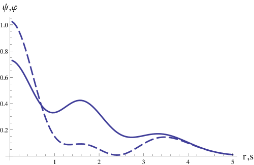
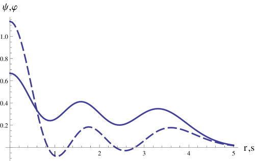
Figure 1: Examples of “positive-positive” and “positive-negative” test functions. Left: both $\psi_{pp}$ (full line), with components, $\{.901,.276,.259,.006,.214\}$, and $\varphi$ (dashed line) are positive. Right: $\psi_{pn}$, with components, $\{.772,.304,.386,.171,.366\}$, remains $>0$ but $\varphi$ takes both signs.

One-dimensional Bochner method

For further discussions, let us denote $\psi_{pp}(r),$ the “positive-positive” (resp. “positive-negative” $\psi_{pn}$) test functions which lead to $\varphi$ positive (resp. not everywhere positive). Figure 1 shows a typical example in each category.

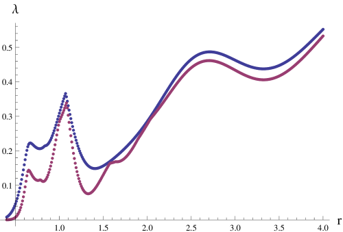
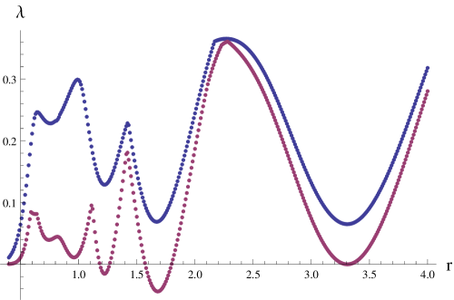
Figure 2: Lowest eigenvalue $\lambda$ as a function of the “grid” parameter $r$ of the Toeplitz matrices, see (36). Upper curves, matrix dimension $5$. Lower curves, matrix dimension $10$. Left: $\psi_{pp}$ case, as described by left part of Fig.1. Right: $\psi_{pn}$ case shown in right part of Fig.1, non positivity of $\varphi$ undetected by dimension $5$, detected by dimension $10$.

Following the results of section IV, all Toeplitz matrices (36) built from $\psi_{pp}(r)$ are positive definite, for all dimensions and for all values of the parameter $r$. None of our numerical tests based on positive-definiteness with our sample of 4388 functions $\psi_{pp}(r)$ contradicted this fact.

According to the same properties, the lack of positive definiteness of the Toeplitz matrix corresponding to the functions $\psi_{pn}(r)$ will show off, sooner or later, for some dimension and some range of $r$. The sign of the Toeplitz determinant, however, may be misleading if an even number of negative eigenvalues occurs. It is safer to track the lowest eigenvalue of a high enough dimensional matrix of the hierarchy (36).

Figure 2 shows, for dimensions $5$ and $10$, how this lowest eigenvalue, $\lambda_{5},\lambda_{10}$, respectively, behaves when $r$ varies when choosing the example functions of Fig.1. Obviously, $\lambda_{10}\leq\lambda_{5},$ since the 5-dimensional Toeplitz matrix is embedded in any higher-dimensional matrix of the hierarchy (36). The left part of Fig.2 considers again that case that was described by the left part of Fig.1. As should be, no negativity is observed, and a confirmation is expected for any matrix dimension. In turn, the right part of Fig.2 describes that case that was illustrated by the right part of Fig.1. No detection occurs if the Toeplitz matrix has only dimension $5$, while dimension $10$ provides a clear detection.

Across our sample of $11068$ cases, a proportion of $\sim 69\%$ are detected with Toeplitz matrices of dimension $5$. With dimension $10$, the success rate reaches $\sim 86\%$. The deeper the negative parts of $\varphi$, the higher the detection probability. However, the “Bochner method” may require for some “rebel” functions a very high dimensionality, and then becomes uneasy. The “Poisson method” will turn out to be easier and with almost full detection success.

One-dimensional Poisson method

Consider the parameter $r$ as an integration grid parameter, $\Delta r$, and also the ratio, $\theta/\Delta r$, as a pseudo momentum, $s$. Using the renormalized definition of the characteristic function (10) and the approximation (19) discussed in subsection III.1, the range of $\psi$ in our samples allows a truncation into a finite sum, namely,

$$F(s,\Delta r)\ \simeq\ \Delta r/\sqrt{2\pi}\,\sum_{n=-K}^{K}\psi(n\Delta r)\ \exp[i(n\Delta r)s]$$ (59)

with $K\simeq R/(\Delta r)$. Here a range $R=10$ is enough to perform a correct coverage of the characteristic function $F(s,\Delta r).$ Note that we thus keep $K\Delta r\simeq R$ constant and look for an integration grid parameter $\Delta r$ not too small, bounded from below, as discussed in subsection III.1.

Contour lines of the values of $F$, in terms of $\Delta r$ and $s$, are shown in Figure 3. Its left and right parts correspond to the “doubly positive” and “partly negative” cases already used for the previous Figures. As expected, no contour for a negative value of $F$ is found for the “doubly positive” case, while “negative contours” occur for the case when $\varphi$ is partly negative. Note, for instance, the “negative” contour line where $F=-0.028$. A few big dots have been plotted to reinforce the visual identification of such “negative” contours.

Such a result, namely a good approximation to a brute force Fourier transform, is expected when $\Delta r$ is small enough to ensure a good convergence, $F(s,\Delta r)\rightarrow\varphi(s)$, but larger values of $\Delta r$ maintain the criterion: negative values of $F$ occur only for non positive $\varphi$’s.

A comment is in thus order: It can be remarked from Fig.3 that the contour curves remain parallel to the abscissa axis for a rather large range of $\Delta r.$ This, joined to the previous remark, can be explained by the fact that the Fourier transform $\varphi(s)$ can be quite well reconstructed from the approximation (59) independently from the value of $\Delta r$ or equivalently of the summation number $K.$ This is exemplified in Figure 4 for the non Fourier-positive function of Fig.1 (right). This is why negative values are reproduced and the test for non Fourier-positivity is successful.

We verified, for $\Delta r$ running between $.1$ and $1$ and $0<s<8$, that our $4388$ “doubly positive” test cases did not generate any negative value of $F$. In turn we verified, for $\Delta r$ running between $.1$ and $1$ and $0<s<8$ again, that most partly negative $\varphi$’s are detected by negative contours. Typically, for $11068$ test cases, only $19$ of them fail generating negative values of $F$ and thus escape detection. An inspection of such “rebel” cases gives a clear explanation for the failure: the negative values of such $\varphi$’s are tiny.

It can be concluded that $F$ provides a very efficient test for the selection of $\psi$ without a detailed calculation of $\varphi$.

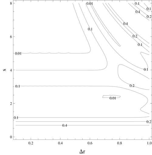
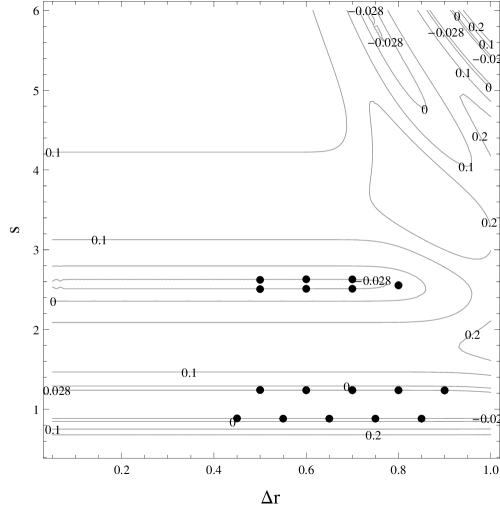
Figure 3: Contour plots of the characteristic function $F$ in terms of the discretization parameter $\Delta r$ and the pseudo-momentum $s\equiv\theta/\Delta r$. Left: Double positivity case, already described by left part of Fig.1. No contour line is found for negative values of $F$. Right: Case already shown in right part of Fig.1, non positivity of $\varphi$ detected by contours for negative values of $F$.

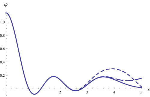
Figure 4: Example of a ‘reconstruction” of a non-Fourier-positive test function. The function $\varphi_{pn}$, depicted in the right part of Fig.1 by a dashed line, is approximated respectively with $K=12$ (small dashes), $K=14$ (large dashes) and $K=20$ (full line, indistinguishable from the true $\varphi_{pn}$.).

V.2 Fourier-Bessel-positivity

Basis of radial functions connected by Bessel transform

Using a similar method as in one dimension, we set a basis, for the functions $\psi$, built from the exponential, $e^{-\frac{x}{2}}$, multiplied by random linear combinations of nine Laguerre polynomials. These are normalized, $\int_{0}^{\infty}x\psi(x)^{2}dx=1$, from the condition, $\sum_{i}c_{i}^{2}=1,$ for the random, real number, mixture coefficients, $c_{i},i=0,\dots,8$. The same coefficients are also selected so that $\psi(x)$ be positive, $\forall x\geq 0.$ The partners in radial momentum space, $\varphi(p)=\int_{0}^{\infty}xJ_{0}(px)\psi(x)dx$, are obtained, with the same coefficients $c_{i}$, from the corresponding basis of functions , also normalized. It is clear that $\varphi(p)$ reads as a polynomial divided by a common denominator, $(1+4p^{2})^{19/2}$. This makes it easy to sort out positive $\varphi$’s from those which take both negative and positive values. We show in Figure 5 a double positivity case (left part) and a case with $\varphi$ partly negative (right part).

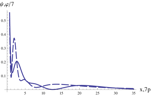
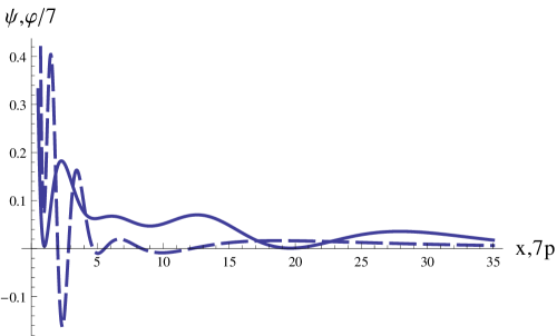
Figure 5: Radial partners under Bessel transform. $\psi$ (full lines) and $\varphi$ (dashes). $Left:$ Fourier-positive case $\psi=e^{-\frac{x}{2}}(3.6096-6.7462x+4.8826x^{2}-1.6141x^{3}+0.28086x^{4}-0.027009x^{5}+0.00145x^{6}-0.000042169x^{7}+5.63539\,10^{-7}x^{8}).$ $Right:$ non Fourier-positive case $\psi=e^{-\frac{x}{2}}(2.49362-6.84573x+6.76697x^{2}-3.04127x^{3}+0.723816x^{4}-0.0959944x^{5}+0.00705616x^{6}-0.000265057x^{7}+3.93896\,10^{-6}x^{8})$. For graphical reasons, the Figure actually shows $\varphi(p/7)/7$.

Our test basis for double positivity contains $185$ cases and that for situations where only $\psi$ remains always positive contains $9894$ cases.

Bochner method for radial functions

It must be kept in mind here that we are in a two-dimensional situation, namely that, given a point with coordinates $\{y,z\}$, the argument $x$ of $\psi$ is, $x=\sqrt{y^{2}+z^{2}}$. Given a list of points $\{y_{i},z_{i}\},i=1,\dots,K$, the matrix elements of the associated, $K$th-order Bochner matrix read, $\psi\left(\sqrt{(y_{i}\!-\!y_{j})^{2}+(z_{i}\!-\!z_{j})^{2}}\right)$. Our numerical tests used a set of points $\vec{r}_{i}$ the coordinates of which, $\{y_{i},z_{i}\}$, are random real numbers in a range, $\{-20,20\}$. A scale parameter, $\beta$, is then introduced to adjust such points to any range $\{-20\beta,20\beta\}$. Typically, we considered the first 20 points, $\{\beta y_{i},\beta z_{i}\}$, with for instance $\beta=.5$, but we also used $\beta=.1$, $\beta=.4$, $\beta=.8$, $\beta=1$. When 20 points gave too few detections, we used as many as $80$ or even $100$ points.

As expected, the Bochner matrices are found positive definite when we investigate the $185$ “doubly positive” cases. In turn, our set of $9884$ test functions for partly negative $\varphi$’s returned a detection rate of $\sim 20\%$ when Bochner matrices of dimension $20$ were used. The rate reached $\sim 40\%$ for matrices of dimension $80$ and hardly increased if $100$ points were used. This modest detection rate with reasonable size matrices contrasts with the good result obtained in the one-dimensional, Gaussian test function case. Matrices of a much higher order are now needed, or a set of more efficient points $\vec{r_{i}}$ must be defined. But we tried several sets of points, different from random ones, and failed to design a “maximum efficiency set of points”.

Fig. 6 shows, for dimensions $20,40,60,80$ respectively, the evolution of the lowest eigenvalue $\lambda$ of a Bochner matrix as a a function of the scale parameter $\beta$. Naturally, the matrix with dimension $20$ being a submatrix of that with dimension $40$, the latter generates a lower bound. The same reasoning applies when the dimension increases, hence the ordering of the four shown curves. The left part of the Figure describes a case where negative values of $\lambda$ are fast obtained. The left part describes a failure case (even for dimension 100).

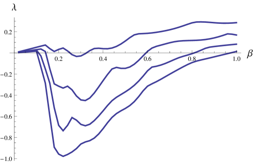
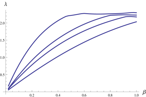
Figure 6: Evolution of the lowest eigenvalue of a Bochner matrix as a function of the scaling parameter $\beta$ for the random points which parametrize the matrix. From top to bottom curve, dimension $20,40,60,80$. Left: the eigenvalue soon becomes negative and detects a partly negative $\varphi$. Right: failure case, where a much larger dimension would be needed for the detection.

Poisson method for radial functions

With the obvious symmetries at our disposal, the Poisson function in this situation can be rewritten as,

$$F(\alpha,\gamma,\Delta r)=(\Delta r)^{2}/(2\pi)\sum_{m=0}^{K}\sum_{k=0}^{K}e_{m}e_{n}\psi\left(\Delta r\sqrt{m^{2}+n^{2}}\right)\cos(m\alpha)\cos(n\gamma)\,,$$ (60)

where, $e_{m}=2-\delta_{m0}$, and the same for $e_{n}$​ , account for edge effects. The range $R$ of $\psi$, typically $R\simeq 40$ for our test functions, provides a natural cut-off, $K\simeq R/\Delta r$, for the $\{m,n\}$ summations. The normalization coefficient, $(\Delta r)^{2}/(2\pi)$, has been introduced to make $F$ similar to a Fourier integral at the limit, $\Delta r\rightarrow 0$.

A similar comment to the one-dimensional case is in order for the radial case. An approximate reconstruction of the Fourier transform function appears to be allowed following formula (19)

Figure 7 shows that, for a finite value of $\Delta r$, hence for finite summations governed by the resulting $K$, negative values of $F$ can be found, even for a “rebel case” like that shown in the right part of Fig. 6. A search for negative values of $F$ under moderate values of $\Delta r$ returns a detection rate of $\sim 90\%$ through our set of 9884 functions. This is significantly better than the result discussed in the previous subsection, where the practical tests based on “Bochner method” appears to be only very slowly evolving with already high matrix order.

Fig.7 calls for a comment. The plots appear to approximately satisfy a radial symmetry in the two-dimensional $(\alpha,\gamma)$ plane, while the resummation formula (60) is not a priori symmetric. The reason is that it gives an approximate reconstruction of the radial function $\varphi(s)$ as predicted by our general argument of section II for the radial 2-dimensional case. This reconstruction property with a finite number of terms in (60) is exemplified in Fig.8 with the non Fourier-positive function depicted in Fig.5. The negative domain is detected already with $K=40$ and reasonably fully reproduced with $K=80.$

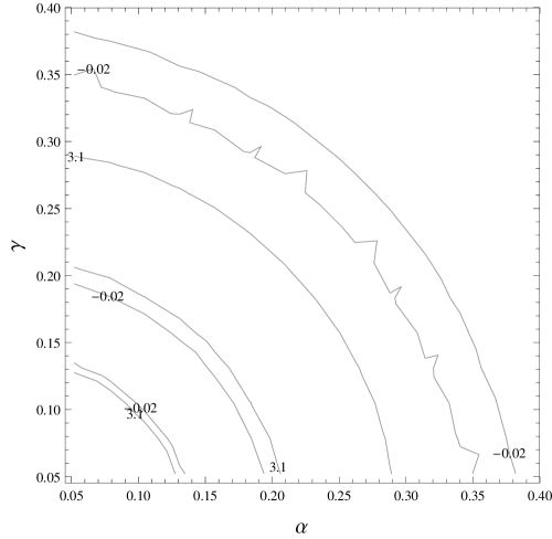
Figure 7: Contour plot of $F(\alpha,\gamma)$ when $\Delta r=.5$. Left: same case as the “success” case shown in the left part of Fig.6; contours for $F=-.3,3$ are shown. Right: same case as the “failure” case shown in the right part of Fig.6; but now, a contour with a negative value, $F=-.02$, provides a detection.

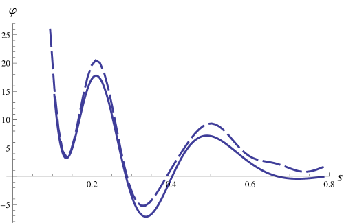
Figure 8: Example of a “reconstruction” of a radial non-Fourier-positive test function. The function $\varphi_{pn}$ depicted in the right part of Fig.5 by a dashed line is approximated respectively with $K=40$ (large dashes, detecting one negative domain) and with $K=80$ (full line, detecting both negative domains).

VI Summary and outlook

In any dimension $d$ there exists a set of real functions, partners under Fourier transform, that are both positive. We have called them Fourier-positive functions. If only for purely mathematical curiosity, the mapping between these two convex, partner sets is of some interest. But this interest is reinforced by the fact that, in theoretical physics, it happens that a “density” in one space has a Fourier partner which is also a “density”. (By definition, densities are positive observables.)

There is also an interesting “subproblem”, that of the mapping between subsets, for instance polynomials multiplied by Gaussians in both spaces, or polynomials multiplied by simple exponentials in one space with rational function partners. Such subsets are nested according to the order of the considered polynomials. This hierarchy allows a useful set of successive approximations.

In fact a general, both necessary and sufficient, mathematical criterion for ensuring Fourier-positivity seems not to be yet known. Indeed, examples taken from physics show that Fourier-positivity is a nontrivial constraint on density models lappi , where small modifications may play a role. For a simple illustration, compare a square well density, whose Fourier transform is the Bessel function, with a Gaussian density, which, being invariant by Fourier transform, is obviously Fourier positive.

Modern computers allow “Fast Fourier Transforms” which give an easy answer to positivity properties in both partner spaces, but, obviously, a pure numerical approach is not completely satisfactory. The present work gives several mathematical, analytical arguments to complement our previous work gipe , where it was shown that the topology of such interesting “positive partner subsets” was highly non trivial and moreover, where there appeared an intuition that extremal elements in such convex sets are reminiscent of Dirac combs.

The proofs displayed in this work do take advantage of this intuition, but indirectly. In substance, we use two kinds of criteria to test whether a positive “object” $\psi$ has a positive “image” $\varphi$, criteria that use values of $\psi$ only. i) A positivy criterion for the characteristic Poisson function associated with $\psi$ through a “Dirac comb” distribution turns out to be quite efficient for both $d=1$ and radial, $d=2$ cases. ii) A criterion taken from Boechner’s theorem, namely the positivity of Toeplitz matrices and similar matrices, turns out to be efficient for $d=1$ cases, but disappointing for radial, d=2 cases. In both cases, we took great care to validate our analytical considerations by means of controled, numerical tests, including statistical evaluations.

A third set of criteria newfourier was in fact our initial approach. It consisted in relating positivity of a function and convexity of analytical continuations of related functions, to define bounds via the Jensen’s theorem, but we failed in making this approach a convincing one, if only because analytical continuation most often has to face severe singularities. It is not displayed in the present work. We keep it on a back-burner.

On a deeper but difficult level, the question of a general criterion of Fourier positivity and a classification of those functions still remains widely open. We hope that the consideration of Dirac combs and Poisson resummation proposed in our paper in this context may help to make some new steps in that problem.

For a more immediate outlook, our priority will be to take advantage of the hierarchy of mapped subspaces abovementioned and use it for actual physical problems. Reliable error bars are essential in data analysis and we want to use our criteria for both estimates of $\psi$ and $\varphi$.

VII Acknowledgements

We want to thank Bertrand Eynard, Philippe Jaming, Jean-Pierre Kahane and Cyrille Marquet for stimulating discussions.

References

- (1)
-
(2)
For a first statement of the problem of Fourier-positivity:
P. Lévy: Fonctions caractéristiques positives [Positive characteristic functions]. Comptes Rendus Hebdomadaires des Séances de l’Académie des Sciences, Série A, Sciences Mathématiques 265 (1967) 249-252. [in French] Reprinted in: Œuvres de Paul Lévy. Volume III. Eléments Aléatoires, edited by D. Dugué in collaboration with P. Deheuvels, M. Ibéro. Gauthier-Villars Éditeur, Paris, 1976, pp. 607-610.
For recent mathematical works:
P. Jaming, M. Matolcsi and S.G. Révész, “On the extremal rays of the cone of positive, positive definite functions,” J. Fourier Anal. Appl., 1, 561 (2009).
A. Hinrichs, J. Vyb ral, “On positive positive-definite functions and Bochner’s Theorem,” J. Complexity 27 , 264, (2011). -
(3)
D. Heck, T. Schlömer and O. Deussen,
“Blue noise sampling with controlled aliasing.”
ACM Trans. Graph. 32,3,25:1, (2013).
S. Pigolotti, C López, E Hernández-García, “Species clustering in competitive Lotka-Volterra models,” Phys. Rev. Lett., 98, 258101 (2007). 2007
F. Baldovin, A.L. Stella, “Central limit theorem for anomalous scaling due to correlations,” Phys. Rev. E, 75(2), 020101, (2007).
T. Lappi “Small x physics and RHIC data,” Int. J. Mod. Phys. E 20, 1, (2011) .
B. Deissler, E. Lucioni, M. Modugno, G. Roati, L. Tanzi, M. Zaccanti, M. Inguscio, and G. Modugno, Correlation function of weakly interacting bosons in a disordered lattice, New J. Phys. 13, 023020 (2011).
C. Cotar, G Friesecke and B. Pass, “Infinite-body optimal transport with Coulomb cost,” arXiv:1307.6540, 2013.
B. G. Giraud and S. Karataglidis, “Algebraic Density Functionals,” Phys. Lett. B 703, 88 (2011). - (4) Y. V. Kovchegov, Phys. Rev. D60, 034008 (1999); Phys. Rev. D61, 074018 (2000).
-
(5)
S. Bochner, Vorlesung über Fouriersche Integrale (Leipzig Verlag,
1932);
English translation: Lectures on Fourier Integrals, Ann. Math. Stud.,
42, (Princeton University Press, 1959).
I.M. Gel’fand and N.Ya. Vilenkin (1968), Generalized Functions, Vol. IV, Academic Press, New-York and London. - (6) B. G. Giraud and R. B. Peschanski, “On positive functions with positive Fourier transforms,” Acta Phys. Polon. B 37, 331 (2006) [math-ph/0504015].
- (7) B. G. Giraud and R. Peschanski, “On the positivity of Fourier transforms,” arXiv:1405.3155 [math-ph].
-
(8)
A. C rdoba, ”La formule sommatoire de Poisson”, C.R. Acad. Sci. Paris,
Series I 306: 373 376.
L. H rmander, The analysis of linear partial differential operators I, Grundl. Math. Wissenschaft. 256, (1983), (Springer, ISBN 3-540-12104-8, MR 0717035). -
(9)
For a review and references including the seminal papers by Akhiezer and Krein on the trigonometric moment problem, see
N.I. Akhiezer, The Classical Moment Problem (Oliver and Boyd, 1965), http://www.maths.ed.ac.uk/ aar/papers/akhiezer.pdf - (10) J.A. Shohat and J.D. Tamarkin, The Problem of Moments, Mathematical Surveys, Number I, (American Mathematical Soc., 1943).
- (11) C. Carathéodory. Über den variabilitätsbereich der fourierschen konstanten von positiven harmonischen funktionen. Rend. Circ. Mat. Palermo, 32, 193-217, 1911.
- (12) O.Toeplitz, Über die Fouriersche Entwicklung positiver Funktionen, Rend. Circ. Mat. Palermo, 32, 1911.
- (13) JB Lasserre, Global optimization with polynomials and the problem of moments, SIAM Journal on Optimization 11 (3), 796-817, and references therein.
- (14) G. Szegö, “Ein Grenzwertsatz ber die Toeplitzschen Determinanten einer reellen positiven Funktion” Math. Ann. , 76 (1915) pp. 490-503; “On certain Hermitian forms associated with the Fourier series of a positive function” Comm. Sem. Math. Univ. Lund (1952) pp. 228-238.
- (15) T. Lappi, “Small x physics and RHIC data,” Int. J. Mod. Phys. E 20, 1 (2011) [arXiv:1003.1852 [hep-ph]].