Multipole modes in deformed nuclei within the finite amplitude method

Abstract

Background

To access selected excited states of nuclei, within the framework of nuclear density functional theory, the quasiparticle random phase approximation (QRPA) is commonly used.

Purpose

We present a computationally efficient, fully self-consistent framework to compute the QRPA transition strength function of an arbitrary multipole operator in axially-deformed superfluid nuclei.

Methods

The method is based on the finite amplitude method (FAM) QRPA, allowing fast iterative solution of QRPA equations. A numerical implementation of the FAM-QRPA solver module has been carried out for deformed nuclei.

Results

The practical feasibility of the deformed FAM module has been demonstrated. In particular, we calculate the quadrupole and octupole strength in a heavy deformed nucleus ²⁴⁰Pu, without any truncations in the quasiparticle space. To demonstrate the capability to calculate individual QRPA modes, we also compute low-lying negative-parity collective states in ¹⁵⁴Sm.

Conclusions

The new FAM implementation enables calculations of the QRPA strength function throughout the nuclear landscape. This will facilitate global surveys of multipole modes and beta decays, and will open new avenues for constraining the nuclear energy density functional.

Introduction – The response of the atomic nucleus to an external perturbation provides valuable information about the underlying nuclear structure and characteristics of the nuclear force Bohr and Mottelson (1975); Lipparini and Stringari (1989); Ring and Schuck (2000); Paar et al. (2007). In addition to nuclear physics aspects, electromagnetic excitations and transition rates have a profound impact on r-process and stellar nucleosynthesis Arnould et al. (2007). Theoretically, a microscopic description of a system with hundreds of strongly interacting fermions is a challenging task. Because exact ab-initio methods are still computationally out of reach for open-shell, heavy systems, self-consistent mean-field models rooted in nuclear density functional theory (DFT) are usually employed when it comes to complex deformed nuclei Ring and Schuck (2000); Bender et al. (2003). The main ingredient of the nuclear DFT is the energy density functional (EDF). Current EDF models have demonstrated the ability to provide a fairly accurate description of nuclear ground state properties across the nuclear chart, despite local deficiencies Bender et al. (2003); Erler et al. (2012); Bogner et al. (2013); Kortelainen et al. (2014).

To access the excited states of nucleus in the framework of nuclear DFT, one of the most straightforward and commonly used method is the linear response theory within random-phase-approximation (RPA) or quasiparticle random-phase-approximation (QRPA). Traditionally, the nuclear QRPA problem has been formulated in a matrix form (MQRPA). Due to large dimension of QRPA matrices, especially when spherical symmetry is broken, fully self-consistent deformed MQRPA calculations have become possible only recently Arteaga and Ring (2008); Terasaki and Engel (2010); Losa et al. (2010); Yoshida (2010); Péru and Goutte (2008); Péru et al. (2011); Yoshida and Nakatsukasa (2011); Martini et al. (2011); Terasaki and Engel (2011); Mustonen and Engel (2013). The large computational cost of deformed MQRPA implies that various truncations of quasi-particle space must be introduced. Such cut-offs, however, break the self-consistency between the underlying Hartree-Fock-Bogoliubov (HFB) solution and QRPA, and may cause an appearance of spurious states.

In order to circumvent various practical deficiencies of MQRPA, a finite amplitude method (FAM) was introduced as a way to compute multipole strength function. With FAM, the QRPA problem is solved iteratively, avoiding costly computation of the MQRPA matrix elements and a subsequent diagonalization. It was first implemented for a computation of the RPA strength function Nakatsukasa et al. (2007), and then applied to a spherically symmetric QRPA Avogadro and Nakatsukasa (2011). In the work of Ref. Stoitsov et al. (2011) the FAM-QRPA was extended to the axially symmetric case within the Skyrme-HFB framework in harmonic oscillator basis. The feasibility of FAM in the framework of relativistic mean field models was studied for the spherical Liang et al. (2013) and axially-symmetric Nikšić et al. (2013) cases. Recently, FAM was also used together with an axially symmetric coordinate-space HFB solver Pei et al. (2014).

The FAM turned out to be a versatile theoretical tool with a broad range of applications in addition to strength function evaluations. For instance, it was demonstrated that it can be used to compute the MQRPA matrix Avogadro and Nakatsukasa (2013); individual QRPA modes Hinohara et al. (2013); sum-rules Hinohara et al. (2015); and $\beta$ decay rates Mustonen et al. (2014). An alternative to FAM to solve the QRPA problem iteratively is the iterative Arnoldi diagonalization scheme, which solves the QRPA equations in a reduced Krylov space Toivanen et al. (2010). This method was also applied to superfluid systems and discrete QRPA states Veselý et al. (2012); Carlsson et al. (2012).

The objective of this work is to extend the FAM to the deformed case, allowing evaluation QRPA modes for operators of arbitrary multipolarity $LK$. This is an extension of our earlier work Stoitsov et al. (2011) that was limited to $K=0$.

Theoretical framework – Our formulation of the FAM-QRPA directly follows that of Ref. Stoitsov et al. (2011) where details can be found. The FAM equations can be written as:

$$\left(E_{\mu}+E_{\nu}-\omega\right)X_{\mu\nu}(\omega)+\delta H^{20}_{\mu\nu}(\omega) = -F^{20}_{\mu\nu},$$ (1a)

$$\left(E_{\mu}+E_{\nu}+\omega\right)Y_{\mu\nu}(\omega)+\delta H^{02}_{\mu\nu}(\omega) = -F^{02}_{\mu\nu},$$ (1b)

where $F^{20}$ and $F^{02}$ are constructed from the external multipole field $f$ that perturbs the system, and $X_{\mu\nu}(\omega)$ and $Y_{\mu\nu}(\omega)$ are the FAM-QRPA amplitudes at a given excitation energy $\omega$. Furthermore, $\delta H^{20}(\omega)$ and $\delta H^{02}(\omega)$ define the response of the nucleus to the external field Stoitsov et al. (2011).

In the original formulation of the FAM, the induced fields were calculated by taking a numerical derivative with respect of a small expansion parameter $\eta$: $\delta h(\omega)=(h[\rho_{\eta},\kappa_{\eta},\bar{\kappa}_{\eta}]-h[\rho,\kappa,\kappa^{*}])/\eta$, $\delta\Delta(\omega)=(\Delta[\rho_{\eta},\kappa_{\eta}]-\Delta[\rho,\kappa])/\eta$, and $\overline{\delta\Delta}(\omega)=(\Delta[\bar{\rho}_{\eta},\bar{\kappa}_{\eta}]-\Delta[\rho,\kappa])/\eta,$ where $\rho$ and $\kappa$ are the HFB particle density and pair density (pairing tensor), respectively, and $\rho_{\eta}$, $\bar{\rho}_{\eta}$, $\kappa_{\eta}$, and $\bar{\kappa}_{\eta}$ are the corresponding FAM densities that depend on $\eta$. In the $K\neq 0$ case considered here, however, the coordinate-space fields $h,\Delta$, and $\overline{\Delta}$ must be linearized explicitly in order not to mix densities with different values of the magnetic quantum number $K$. Such a linearization is possible since the oscillating part of the density, proportional to $\eta$, is assumed to be small compared to the static HFB density. Due to this explicit linearization, the expansion parameter $\eta$ is no longer needed and the induced densities are:

$$\rho_{\rm f} = +UXV^{T}+V^{*}Y^{T}U^{{\dagger}},$$ (2a)

$$\bar{\rho}_{\rm f} = +V^{*}X^{{\dagger}}U^{{\dagger}}+UY^{*}V^{T},$$ (2b)

$$\kappa_{\rm f} = -UX^{T}U^{T}-V^{*}YV^{{\dagger}},$$ (2c)

$$\bar{\kappa}_{\rm f} = -V^{*}X^{*}V^{{\dagger}}-UY^{{\dagger}}U^{T}\,,$$ (2d)

where $U$ and $V$ are the usual HFB matrices, and the subscript f indicates oscillating densities induced by the external field atop of the static HFB density. The linearized fields are: $\delta h(\omega)=h[\rho_{\rm f},\kappa_{\rm f},\bar{\kappa}_{\rm f}]$, $\delta\Delta(\omega)=\Delta[\rho_{\rm f},\kappa_{\rm f}]$, and $\overline{\delta\Delta}(\omega)=\Delta[\bar{\rho}_{\rm f},\bar{\kappa}_{\rm f}].$ In practice, for Skyrme-like EDFs, the explicit linearization is required for the density-dependent fields.

In implementation of the new FAM module, we have utilized the simplex-$y$ ($\hat{S}_{y}$) symmetry Dobaczewski et al. (2000). Consequently, the basis states used are eigenstates of $\hat{S}_{y}$ operator corresponding to eigenvalues of $+i$ and $-i$; they can be written as combinations of $|+\Omega\rangle$ and $|-\Omega\rangle$ states, where $\Omega$ is the projection of the single-particle angular momentum along the $z$-axis Goodman (1974). With a proper selection of the operator $f$ for the external field, basis states with opposite simplex eigenvalues are not connected by the induced density matrix $\rho_{\rm f}$. In a $K\neq 0$ case, the density matrix has a block structure, dictated by the operator $f$, corresponding to the selection rule $\Delta\Omega=K$.

In terms of FAM-QRPA amplitudes, the multipole strength can be expresses as:

$$\frac{dB(\omega;F)}{d\omega}=-\frac{1}{\pi}{\rm Im\,Tr}\left[f(UXV^{T}+V^{*}Y^{T}U^{{\dagger}})\right].$$ (3)

To guarantee that the FAM-QRPA solution has finite strength, a small imaginary component is introduced to the excitation energy $\omega$ as $\omega\,\to\,\omega+i\gamma$ Nakatsukasa et al. (2007). Actually, the position of $\omega$ in the complex plane does not need to be limited to this particular choice: by choosing a suitable integration contour in the complex-$\omega$ plane, discrete QRPA states or sum rules can be obtained Hinohara et al. (2013, 2015).

The electric isoscalar (IS) and isovector (IV) multipole operators are Lipparini and Stringari (1989):

$$f^{\rm IS}_{LK}=e_{\rm IS}\sum_{i=1}^{A}{f}_{LK}(\mbox{\boldmath$r$}_{i}),~{}f^{\rm IV}_{LK}=\sum_{i=1}^{A}e_{{\rm IV},\tau_{i}}\tau_{i}{f}_{LK}(\mbox{\boldmath$r$}_{i}),$$ (4)

where $\tau_{i}=\pm 1$ for neutrons/protons, $f_{LK}(\mbox{\boldmath$r$})=r^{L}{Y}_{LK}(\hat{\mbox{\boldmath$r$}})$, and $e_{\rm IS}$ and $e_{{\rm IV},\tau_{i}}$ are isoscalar and isovector effective charges, respectively. As simplex-$y$ is considered to be a self-consistent symmetry, one can replace

$$f_{LK}\rightarrow f^{+}_{LK}=\left(f_{LK}+f_{L,-K}\right)/\sqrt{2-\delta_{K0}}$$ (5)

and assume $K\geq 0$ in the following. Indeed, for an even-even axial nucleus, operators $f_{LK}$ and $f_{L,-K}$ produce identical strength functions.

Our FAM-QRPA implementation is based on the DFT code hfbtho Stoitsov et al. (2013), which solves the HFB equations in axially symmetric (transformed) harmonic oscillator basis by assuming time-reversal symmetry. The iterative Broyden method of Ref. Baran et al. (2008) is used to speed up the convergence of the FAM-QRPA iterations. For the direct Coulomb part, we use the same method as in the version v200d of hfbtho Stoitsov et al. (2013), generalized to the $K\neq 0$ case. We benchmarked the new FAM code against the old FAM module of Ref. Stoitsov et al. (2011) in the case of monopole and quadrupole modes with $K=0$, and obtained perfect agreement. For the negative-parity electric operators, the used coordinate mesh also included the half-volume corresponding to negative-$z$ values.

We would like to stress that, unlike in the standard deformed MQRPA, we do not impose any kind of truncation on the quasiparticle FAM-QRPA space. The only cut-off (besides the size of the harmonic oscillator basis) is the employed pairing window used for the calculation of induced densities, in order to keep self-consistency with respect to the underlying HFB calculation.

The calculation of the FAM strength function can be trivially parallelized by distributing parts of the strength function over multiple CPU cores. To this end, we have implemented a parallel MPI calculation scheme. In practice, a computation of a typical strength function with 20 oscillator shells, and without the reflection symmetry assumed, on a multicore Intel Sandy Bridge 2.6 GHz processor system, takes about 1000 CPU hours.

Results – In our illustrative examples, we have used two Skyrme EDF parameterizations, SkM* Bartel et al. (1982) and SLy4 Chabanat et al. (1995). Both parameterizations have been found to be stable to linear response in infinite nuclear matter Pastore et al. (2012).

In a spherical nucleus, the strength function for a given multipole $L$ does not depend on $K$ quantum number. This offers a stringent test of our numerical implementation of the FAM module. To this end, we computed the isovector quadrupole strength for ²⁰O, with SkM* Skyrme EDF, in a space of $N_{\rm sh}=15$ oscillator shells, by using mixed pairing interaction with strength of $V_{0}=-280\,{\rm MeV\,fm^{3}}$ and a quasiparticle cut-off of 50 MeV. The setup of this calculation was the same as in the MQRPA calculation of Ref. Losa et al. (2010) to facilitate comparison. We confirmed that the transition strengths of all $K$-modes coincide, and the results agree very well with those of Ref. Losa et al. (2010). The relative differences between various $K$-modes in our calculations were typically at the level of $\mathcal{O}(10^{-5})$, or smaller.

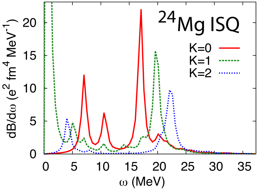
Figure 1: (Color online) Isoscalar quadrupole strength in the prolate deformed configuration of ²⁴Mg calculated with SkM* EDF and $N_{\rm sh}=15$.

Figure 1 shows the calculated isoscalar quadrupole transition strength in ²⁴Mg. The calculation was done by using the same setup as in the case of ²⁰O. Here, we consider the deformed configuration of ²⁴Mg with quadrupole deformation $\beta=0.39$. In this configuration, static pairing vanishes for both protons and neutrons. Due to the deformation, strength functions of different $K$-modes differ. By comparing our results with those of Ref. Losa et al. (2010), we again find excellent agreement, except for the spurious reorientation Nambu-Goldstone $K=1$ mode that shows up just above $\omega=0$. For more discussion of spurious modes in FAM-QRPA we refer the reader to the recent paper Hinohara (2015).

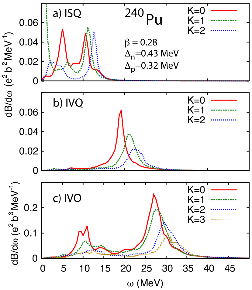
Figure 2: (Color online) Isoscalar (a) and isovector (b) quadrupole strengths, and isovector octupole strength (c) in ²⁴⁰Pu calculated with SLy4 EDF and $N_{\rm sh}=20$.

To demonstrate the performance of the new FAM module for deformed heavy nuclei, we calculated the quadrupole and octupole transition strengths in ²⁴⁰Pu. The results obtained with 20 oscillator shells are presented in Fig. 2, which shows a typical pattern dominated by the presence of giant quadrupole (GQR) and giant octupole (GOR) resonances. In this case we used SLy4 EDF together with a mixed pairing force with a strength of $V_{0}=-283.45\,{\rm MeV\,fm^{3}}$. The resulting HFB state had deformation $\beta=0.28$, and pairing gaps $\Delta_{\rm n}=0.43\,{\rm MeV}$ and $\Delta_{\rm p}=0.32\,{\rm MeV}$.

Our calculations predict the $K$-splitting of the multipole strength due to deformation. For the IS-GQR, the splitting follows the pattern predicted by phenomenological models Kishimoto et al. (1975); Lipparini and Stringari (1981); Nishizaki and Andō (1985), i.e., for the prolate deformations the ISGQR energy increases with $K$. A similar hierarchy is predicted for IV-GQR and IV-GOR. The mean GQR energies shown in Figs. 2(a) and (b) are consistent with the values predicted in the recent time-dependent DFT calculations of Ref. Scamps and Lacroix (2014) and the MQRPA study of Ref. Péru et al. (2011). The latter work also contains predictions for the octupole response in the neighboring nucleus ²³⁸U. Similar as in Fig.  2(c), they predict a strong fragmentation of low-energy and high-energy octupole strength. The mean energy of the high-energy IVGOR predicted in our work, around 28 MeV, agrees well with the early predictions of Ref. Malov et al. (1976). Once again, for the isoscalar quadrupole mode with $K=1$, we find a spurious state related to the rotational Nambu-Goldstone mode. In addition, we have also tested that, by using a stretched harmonic oscillator basis, the new FAM module can be employed to compute the multipole strength in the fission isomer of ²⁴⁰Pu.

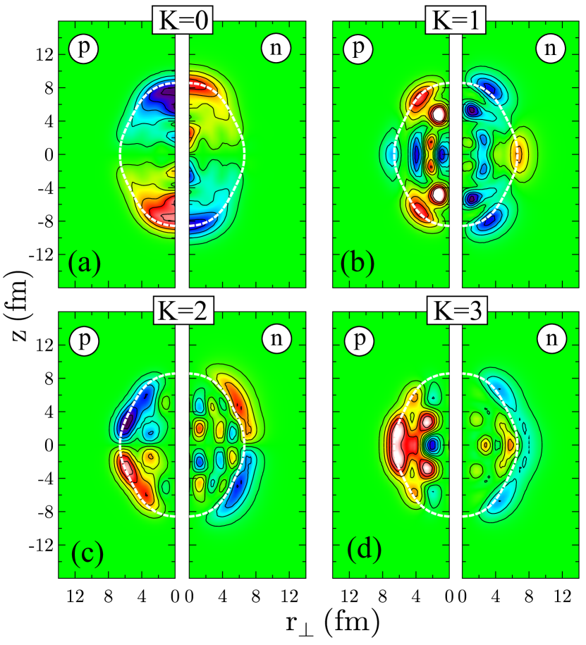
Figure 3: (Color online) The imaginary part of the induced IVO transition density $\rho_{\rm f}$ at the excitation energy $\omega=11$ MeV for protons and neutrons in ²⁴⁰Pu. All $K$-modes have been normalized in the same way: Red color indicates the maximum (positive) value for each mode and blue color indicates the minimum (negative) value. The white dashed line indicates the contour of $\rho_{\rm n}+\rho_{\rm p}=0.08\,{\rm fm}^{-3}$ obtained from the HFB calculation.

To shed light on the spatial structure of induced transition density, we show in Fig. 3 the induced proton and neutron IVO transition densities in ²⁴⁰Pu, for all the $K$-modes, at $\omega=11$ MeV. Owing to the isovector character of the mode, protons and neutrons exhibit out-of-phase oscillations. Furthermore, the spatial transition densities show a clear octupole pattern. The transition densities cover a significant portion of the nuclear volume; this reflects the collective character of the mode.

Finally, we demonstrate the capability of the new FAM module to compute the discrete QRPA modes. The samarium and neodymium isotopes around $A=150$ are known to exhibit low-energy octupole modes. We have chosen an octupole-stable isotope ¹⁵⁴Sm and calculated the low-lying octupole vibrational states, using the same computational setup as for ²⁴⁰Pu. The ground-state quadrupole deformation predicted in HFB was $\beta=0.32$, and the pairing gaps were $\Delta_{\rm n}=0.30$ MeV and $\Delta_{\rm p}=0.53$ MeV. The calculation was carried out by using the contour integration technique of Ref. Hinohara et al. (2013) and by applying an external isovector octupole field to extract the individual states. To confirm our results, we repeated the calculations by using the isovector dipole ($K=0$ and 1) and isoscalar octupole ($K=2$ and 3) fields. Table 1 displays the isovector octupole transition strengths and corresponding proton $B$(E3) values. The $K=0$ and 1 excited states carry the octupole strength that is larger than 1 W.u., indicating their collective nature.

Experimentally, two negative parity rotational bands with the band heads of $J^{\pi}=1^{-}$, 921.3 keV and $J^{\pi}=1^{-}$, 1475.8 keV have been identified in ¹⁵⁴Sm. Those bands have been associated with $K^{\pi}=0^{-}$ and $1^{-}$ octupole vibrations, respectively. Although our calculation underestimates the experimental excitation energies of these states, the $B$(E3) value of the $K^{\pi}=0^{-}$ state agrees well with the experimental value $B$(E3;$0_{1}^{+}\to 3_{1}^{-})=10(2)$ W.u. Spear (1989). The excitation energies of the lowest $K^{\pi}=0^{-}$ and $1^{-}$ excited states in ¹⁵⁴Sm are also presented in Ref. Yoshida and Nakatsukasa (2011), and their values obtained with MQRPA with SkM* EDF are higher than ours. The translational spurious modes appear at $\omega=0.11$ MeV ($K^{\pi}=0^{-}$) and $\pm$0.17$i$ MeV ($K^{\pi}=1^{-}$), and since the lowest $K^{\pi}=0^{-}$ collective state is close to the spurious mode, some contamination due to the spurious components is expected. We are in the process of implementing the prescription proposed in Ref. Nakatsukasa et al. (2007) to remove the spurious components from FAM-QRPA modes.

Table 1: Lowest octupole QRPA modes in ¹⁵⁴Sm predicted in our deformed FAM calculations. Shown are: the energy $\omega_{1}$; the IVO transition strength $|\langle 0|f^{IV,+}_{L=3,K}|1\rangle|^{2}$; and the corresponding $B$(E3) value. The transition probabilities were computed through the QRPA amplitudes (referred to as FAM-C in Hinohara et al. (2013)).

$K$	$\omega_{1}$	$|\langle 0|f^{IV,+}_{L=3,K}|1\rangle|^{2}$	$B$(E3)
	(MeV)	($e^{2}$fm6 MeV${}^{-1})$	(W.u.)
0	0.4168	6.684	8.70
1	0.9014	69.74	2.01
2	2.5973	1.916	0.24
3	1.3155	0.01809	0.0004

Conclusions – In this work we have introduced the FAM-QRPA method suitable for calculation of an arbitrary multipole strength function in axially deformed superfluid nuclei. The method allows a fast calculation of the strength function without any additional truncations in the quasiparticle space. The method has been benchmarked in spherical and deformed nuclei by comparing with earlier MQRPA calculations Losa et al. (2010). To demonstrate the applicability of the method to heavy deformed nuclei, we calculated quadrupole and octupole strength functions in ²⁴⁰Pu. We also showed that the deformed FAM module can be used to compute discrete QRPA modes.

Since the majority of nuclei are predicted to be axially deformed in their ground states, the proposed FAM-QRPA method is a tool of the choice to study the linear multipole response across the nuclear landscape. Large-scale surveys with the deformed FAM-QRPA approach can be carried out very efficiently as the method is amendable to parallel computing. Another useful application is in the area of EDF optimization, where new experimental information on multipole strength in deformed nuclei can be used to better constrain the isovector sector of the effective interaction.