Electric quadrupole and magnetic dipole moments of odd nuclei
near the magic ones in a self-consistent approach

Abstract

We present a model which describes the properties of odd-even nuclei with one nucleon more, or less, with respect to the magic number. In addition to the effects related to the unpaired nucleon, we consider those produced by the excitation of the closed shell core. By using a single particle basis generated with Hartree-Fock calculations, we describe the polarization of the doubly magic-core with Random Phase Approximation collective wave functions. In every step of the calculation, and for all the nuclei considered, we use the same finite-range nucleon-nucleon interaction. We apply our model to the evaluation of electric quadrupole and magnetic dipole moments of odd-even nuclei around oxygen, calcium, zirconium, tin and lead isotopes. Our Random Phase Approximation description of the polarization of the core improves the agreement with experimental data with respect to the predictions of the independent particle model. We compare our results with those obtained in first-order perturbation theory, with those produced by Hartree-Fock-Bogolioubov calculations and with those generated within the Landau-Migdal theory of finite Fermi systems. The results of our universal, self-consistent, and parameter free approach have the same quality of those obtained with phenomenological approaches where the various terms of the nucleon-nucleon interaction are adapted to reproduce some specific experimental data. A critical discussion on the validity of the model is presented.

I Introduction

The description of the angular momenta of odd-even nuclei is one of the greatest successes of the nuclear shell-model. The angular momentum and the parity of the single particle (s.p.) level of the unpaired nucleon correspond to those of the whole nucleus. This extreme shell model picture, where the s.p. properties are imposed to the whole interacting many-body system, is weakened when observables which are not quantized are investigated. For example, the values of electric quadrupole and magnetic dipole moments are rather different from those predicted by the extreme shell model. For these quantities, the interaction between the unpaired nucleon and the other nucleons plays an important role, strongly modifying the pure shell model predictions.

One expects that in odd-even nuclei around doubly-magic ones, the effects related to the extreme shell model picture, which we shall name henceforth Independent Particle Model (IPM), are dominant with respect to those induced by the two-body part of the nuclear hamiltonian, usually called residual interaction. This has induced the development of various perturbative models goo72 ; ell77 . A class of these models is based on the straightforward application of the traditional perturbation theory, which, however, has convergence problems, at least for the terms beyond those of the first order li13 .

Another perturbative approach consists in considering the residual interaction within the framework of the Random Phase Approximation (RPA) theory. This approach is based on the extension of the Landau theory of quantum liquids to finite Fermi systems (FFS) done by Migdal mig67 . This theory has been applied with great success to describe the properties of odd-even nuclei in the region of ²⁰⁸Pb rin73 ; bau73 ; spe77 . In these works the s.p. wave functions are generated by diagonalizing a Woods-Saxon well, and the residual interaction is a zero-range Landau-Migdal force mig67 . More recently, this approach has been extended to use the same interaction in the production of the s.p. wave functions and in the RPA calculations bor08 ; bor10 ; tol11 ; tol12 ; voi12 . Furthermore, also pairing effects have been considered. This self-consistent theory of FFS has been applied also to the tin and to the calcium isotopes. In these approaches, the use of the concept of quasi-particles implies the definition of the effective charge which contains free parameters whose values are chosen to have a good description of the data. In the phenomenological approach of Refs. rin73 ; bau73 ; spe77 also the constants defining the strength of the various channels of the Landau-Migdal nucleon-nucleon effective interaction have been used as free parameters. In this case, the values of these parameters are related to the dimension of the s.p. configuration space. The application of these methods to a different region of the nuclear chart, or, more simply, to a different s.p. configuration space, requires a new selection of the free parameter values. The self-consistent FFS approach of Refs. bor08 ; bor10 ; tol11 ; tol12 ; voi12 does not have cut-off problems in the RPA calculations, since it considers the full s.p. configuration space, continuum included. The problems arise in the pairing calculations, where the free parameter is the value of the cutoff energy used as regulator, in analogy to the renormalisation procedure adopted in effective field theories.

Inspired by these works, we propose here an extension of the RPA formalism to construct a fully self-consistent approach. For each nucleus considered, we use a set of s.p. wave functions generated by a Hartree-Fock (HF) calculation. The same, effective, nucleon-nucleon interaction used in HF is adopted in the RPA calculations, which allows the evaluation of the odd-even nucleus observables. The parameters of the force, which we consider having finite-range, have been chosen once forever in a global HF fit of properties mainly related to the ground state of a large set of nuclei in all the regions of the nuclear chart cha07t . The use of a finite-range interaction ensures the stability of our results whose values, after convergence has been reached, do not depend any more on the size of the s.p. configuration space.

The basic ideas of our work are relatively simple and straightforward. First, we use effective nucleon-nucleon interactions whose parameters have been chosen to reproduce data which are not directly related to the observables we investigate. Second, the chain of calculations needed to arrive at the final results does not contain any additional free parameter, but they depend exclusively on the effective nucleon-nucleon interaction. To be sure of identifying features related to the theory, and not to the specific choice of the interaction or to the nucleus investigated, we carried out calculations with different nucleon-nucleon forces, for a set of nuclei in a large region of the nuclear chart. We mainly concentrate our investigation on two observables, the electric quadrupole, $Q$, and the magnetic dipole, $\mu$, moments of a selected set of odd-even nuclei. The evaluation of these quantities requires, respectively, the description of the $2^{+}$ and $1^{+}$ excitations of the even-even core nuclei which we obtain by using a RPA approach don14a .

In Sec. II we present the basic ideas our model. In this section we also specify the form of the electromagnetic operators that we have adopted to describe $Q$ and $\mu$. The expression of the operator for $Q$ is simple and straightforward. More complex is the situation for $\mu$, where, in addition to the traditional one-body operator, we consider also two-body currents generated by the exchange of charged pions. We shall refer to these latter currents as meson exchange currents (MEC). In Sec. III we discuss some details of the calculations related to the specific applications of the model. The results obtained for $Q$ and $\mu$ are presented in Sect. IV. In both cases we also study the excitation of the even-even core nuclei for the two multipolarities involved. In Sec. V we summarize the main results of our study, and we draw our conclusions.

II The model

The starting point of our model is the construction of the basis of s.p. states $|\phi_{\alpha}\rangle$, which we generate by solving the HF equations. We used the symbol $\alpha$ to indicate all the quantum numbers characterizing the s.p. state, i.e. the principal quantum number $n_{\alpha}$, the orbital angular momentum $l_{\alpha}$, the total angular momentum $j_{\alpha}$, its third component $m_{\alpha}$, and the third component of the isospin $t_{\alpha}=-1/2$ for protons, and $t_{\alpha}=1/2$ for neutrons.

In the IPM picture, all the s.p. states below the Fermi energy are completely occupied, and those above it are empty. We indicate with $|\Phi_{0}\rangle$ the Slater determinant describing the IPM ground state of the doubly magic nucleus composed by $A$ nucleons. By definition, the RPA ground state of the doubly magic nucleus, which we indicate as $|\Psi_{0}\rangle$, contains correlations beyond the IPM.

The odd-even nuclei we want to describe are obtained by adding, or subtracting, one nucleon to the doubly-magic $A$-nucleon system. We label the states of these nuclei as $|A\pm 1;\alpha\rangle$, where the symbol $\alpha$ indicates the set of quantum numbers characterizing the s.p. state of the added, or subtracted, nucleon.

We describe the response of the odd-even nucleus to the perturbation induced by an external operator ${\cal B}$ by considering separately two effects. The first one is the action of the external operator on the unpaired nucleon, while the doubly-magic core remains unperturbed. The second effect considers the interaction of the external probe with one of the nucleons of the doubly magic core. In this case, the whole nucleus responds to the external perturbation because the nucleon struck by the external probe interacts strongly with all the other nucleons, included the unpaired one.

We express the expectation value of the external operator ${\cal B}$ between two states of the odd-even nucleus with one nucleon more than the doubly-magic one as mig67 ; rin73 ; bau73 ; spe77

$$\langle\,A+1;\alpha\,|\,{\cal B}\,|\,A+1;\beta\,\rangle\,=\,\langle\,\Phi_{0}\,|\,a_{\alpha}\,{\cal B}\,a^{+}_{\beta}\,|\,\Phi_{0}\,\rangle\,+\,\langle\,\Psi_{0}\,|\,a_{\alpha}\,a^{+}_{\beta}\,V_{\rm res}\,{\cal P}_{A}(\epsilon_{\alpha\beta})\,{\cal B}\,|\,\Psi_{0}\,\rangle\,,$$ (1)

where $a^{+}$ and $a$ are the usual creation and annihilation operators, $V_{\rm res}$ is the residual nucleon-nucleon interaction, and ${\cal P}_{A}$ is a propagator which describes the excitation of the doubly magic core and depends on $\epsilon_{\alpha\beta}=\epsilon_{\alpha}-\epsilon_{\beta}$, the difference between the energies of the two states of the $A+1$ system. A similar equation can be written for the $A-1$ nucleus by exchanging creation and annihilation operators.

In our approach, the excitation of the doubly magic core is described by using the RPA theory. In terms of an excitation operator $Q^{+}_{\nu}$, we define the excited states of the $A$-nucleon system as

$$|\,\Psi_{\nu}\,\rangle\,=\,Q^{+}_{\nu}\,|\,\Psi_{0}\,\rangle\,,$$ (2)

while the relation

$$Q_{\nu}\,|\,\Psi_{0}\,\rangle\,=\,0$$ (3)

defines the ground state. The label $\nu$ indicates all the quantum numbers needed to characterize the excited state. The RPA excitation operator is defined as

$$Q^{+}_{\nu}\,=\,\sum_{ph}\,\left(\,X^{\nu}_{ph}\,a^{+}_{p}\,a_{h}\,-\,Y^{\nu}_{ph}\,a^{+}_{h}\,a_{p}\,\right)\,,$$ (4)

where the index $p$ refers to s.p. states above the Fermi surface (particles) and $h$ to s.p. states below it (holes). The RPA propagator can be written as mig67 ; spe77 ; fet71

$${\cal P}^{\rm RPA}_{A}(\epsilon_{\alpha\beta})\,=\,\sum_{\nu}\,Q^{+}_{\nu}\,|\,\Psi_{0}\,\rangle\,\left(\,\frac{1}{\epsilon_{\alpha\beta}\,-\,\omega_{\nu}}\,-\,\frac{1}{\epsilon_{\alpha\beta}\,+\,\omega_{\nu}}\,\right)\langle\,\Psi_{0}\,|\,Q_{\nu}\,,$$ (5)

where $\omega_{\nu}$ is the excitation energy of the state $|\,\Psi_{\nu}\,\rangle$. By using this propagator, we express the second term in the r.h.s. of Eq. (1) as

$$\langle\,\Psi_{0}\,|\,a_{\alpha}\,a^{+}_{\beta}\,V_{\rm res}\,{\cal P}^{\rm RPA}_{A}(\epsilon_{\alpha\beta})\,{\cal B}\,|\,\Psi_{0}\,\rangle =$$

$$=\,\langle\,\Psi_{0}\,|\,a_{\alpha}\,a^{+}_{\beta}\,V_{\rm res}\,\sum_{\nu}\,Q^{+}_{\nu}\,|\,\Psi_{0}\,\rangle\,\left(\,\frac{1}{\epsilon_{\alpha\beta}\,-\,\omega_{\nu}}\,-\,\frac{1}{\epsilon_{\alpha\beta}\,+\,\omega_{\nu}}\,\right)\,\langle\,\Psi_{0}\,|\,Q_{\nu}\,{\cal B}\,|\,\Psi_{0}\,\rangle$$

$$=\,\sum_{\nu}\,\langle\,\Psi_{0}\,|\,\left[\,a_{\alpha}\,a^{+}_{\beta}\,V_{\rm res}\,,Q^{+}_{\nu}\,\right]\,|\,\Psi_{0}\,\rangle\left(\,\frac{1}{\epsilon_{\alpha\beta}\,-\,\omega_{\nu}}\,-\,\frac{1}{\epsilon_{\alpha\beta}\,+\,\omega_{\nu}}\,\right)\,\langle\,\Psi_{0}\,|\,\left[\,Q_{\nu}\,,{\cal B}\,\right]\,|\,\Psi_{0}\,\rangle\,,$$

where we have exploited Eq. (3) to insert the commutator $[\,,]$ between operators, with the aim of using the quasi-boson-approximation rin80 :

$$\langle\,\Psi_{0}\,|\,a_{\alpha}\,a^{+}_{\beta}\,V_{\rm res}\,{\cal P}^{\rm RPA}_{A}(\epsilon_{\alpha\beta})\,{\cal B}\,|\,\Psi_{0}\,\rangle \simeq$$

$$\simeq\,\sum_{\nu}\,\langle\,\Phi_{0}\,|\,\left[\,a_{\alpha}\,a^{+}_{\beta}\,V_{\rm res}\,,Q^{+}_{\nu}\,\right]\,|\,\Phi_{0}\,\rangle\left(\,\frac{1}{\epsilon_{\alpha\beta}\,-\,\omega_{\nu}}\,-\,\frac{1}{\epsilon_{\alpha\beta}\,+\,\omega_{\nu}}\,\right)\,\langle\,\Phi_{0}\,|\,\left[\,Q_{\nu}\,,{\cal B}\,\right]\,|\,\Phi_{0}\,\rangle\,.$$

The operator describing the action of the external probe on the nuclear system can be expressed in terms of a multipole expansion. Each term of this expansion, ${\cal B}_{JM}$, is characterized by the angular momentum $J$, and its projection $M$ on the quantization axis. In our calculations we consider the spherical symmetry of the problem. We use a set of s.p. wave functions with the following angular momentum coupling structure:

$$\phi_{\alpha}({\bf r})\,=\,R^{t_{\alpha}}_{n_{\alpha}l_{\alpha}j_{\alpha}}(r)\,\sum_{\mu_{\alpha}s_{\alpha}}\,\langle\,l_{\alpha}\,\mu_{\alpha}\,\frac{1}{2}\,s_{\alpha}\,|\,j_{\alpha}\,m_{\alpha}\,\rangle\,Y_{l_{\alpha}\mu_{\alpha}}(\theta,\phi)\,\chi_{s_{\alpha}}\,,$$ (8)

where $(r,\theta,\phi)$ are the usual polar coordinates, $Y_{l\mu}$ are the spherical harmonics, $\chi$ the Pauli spinor, and the symbol $\langle|\rangle$ indicates the Clebsch-Gordan coefficient. We calculate the matrix elements by applying the Wigner-Eckart theorem with the phase conventions of Ref. edm57 , and we sum on all the possible values of $m_{\alpha}$ and $m_{\beta}$. For the matrix element in Eq. (1) we obtain

$$\langle\,A+1;\alpha\,||\,{\cal B}_{J}\,||\,A+1;\beta\,\rangle =$$

$$=\,\langle\,\phi_{\alpha}\,||\,{\cal B}_{J}\,||\,\phi_{\beta}\,\rangle\,+\,\delta_{\alpha,\beta}\,\sum_{h}\,\langle\,\phi_{h}\,||\,{\cal B}_{J}\,||\,\phi_{h}\,\rangle$$

$$+\,\sum_{\nu}\,\Big{[}\,{\cal D}^{\nu}_{\alpha\beta}\,\sum_{ph}\,{\cal A}_{ph}^{\nu}\,\langle\,\phi_{p}\,||\,{\cal B}_{J}\,||\,\phi_{h}\,\rangle\,+\,{\cal G}^{\nu}_{\alpha\beta}\,\sum_{ph}\,(-1)^{j_{h}+j_{p}}\,{\cal A}_{ph}^{\nu}\,\langle\,\phi_{p}\,||\,{\cal B}_{J}\,||\,\phi_{h}\,\rangle\Big{]}\,,$$

where the two kernels are defined as

$${\cal D}^{\nu}_{\alpha\beta}\,=\,\sum_{ph}v^{J}_{\alpha\beta ph}\left(\frac{X^{\nu}_{ph}}{\epsilon_{\alpha\beta}-\omega_{\nu}}+(-1)^{j_{h}+j_{p}}\frac{Y^{\nu}_{ph}}{\epsilon_{\alpha\beta}+\omega_{\nu}}\right)$$ (10)

and

$${\cal G}^{\nu}_{\alpha\beta}\,=\,\sum_{ph}v^{J}_{\alpha\beta hp}\left(\frac{X^{\nu}_{ph}}{\epsilon_{\alpha\beta}+\omega_{\nu}}+(-1)^{j_{h}+j_{p}}\frac{Y^{\nu}_{ph}}{\epsilon_{\alpha\beta}-\omega_{\nu}}\right)\,,$$ (11)

with

$${\cal A}_{ph}^{\nu}\,=\,X^{\nu}_{ph}\,+\,(-1)^{j_{h}-j_{p}}\,Y^{\nu}_{ph}\,.$$ (12)

In Eq. (II) the double bars indicate that in the matrix elements between the two s.p. wave functions the angular part is evaluated in terms of reduced matrix elements. The calculation of the radial integrals is understood.

The expression of the interaction terms $v^{J}$ is analogous to that of the RPA fet71

$$v^{J}_{\alpha\beta\gamma\delta} = \sum_{K}\,(-1)^{K+j_{\beta}+j_{\delta}}\,\widehat{K}\,\left\{\begin{array}[]{ccc}j_{\alpha}&j_{\beta}&J\\ j_{\delta}&j_{\gamma}&K\end{array}\right\}$$ (16)

$$\times\,\Big{[}\langle\,j_{\alpha}\,j_{\gamma}\,K\,\|\,V_{\rm res}\,\|\,j_{\beta}\,j_{\delta}\,K\,\rangle\,-\,(-1)^{j_{\beta}+j_{\delta}-K}\,\langle\,j_{\delta}\,j_{\beta}\,K\,\|\,V_{\rm res}\,\|\,j_{\alpha}\,j_{\gamma}\,K\,\rangle\Big{]}\,.$$

In the above equation we used the Wigner 6-$j$ symbol edm57 , and $\widehat{j}\equiv\sqrt{2j+1}$, where $j$ is referred to an angular momentum. The interaction $V_{\rm res}$ is described as

$$V_{\rm res} = v_{1}({r_{ij}})\,+\,v_{2}({r_{ij}})\,{\boldsymbol{\tau}(i)\cdot\boldsymbol{\tau}(j)}\,+\,v_{3}({r_{ij}})\,{\boldsymbol{\sigma}(i)\cdot\boldsymbol{\sigma}(j)}\,+\,v_{4}({r_{ij}})\,{\boldsymbol{\sigma}(i)\cdot\boldsymbol{\sigma}(j)}\,{\boldsymbol{\tau}(i)\cdot\boldsymbol{\tau}(j)}$$

$$+\,t_{\rho}\left[1-{\boldsymbol{\tau}(i)\cdot\boldsymbol{\tau}(j)}\right]\,\rho^{1/3}\,\left(\frac{r_{i}+r_{j}}{2}\right)\delta({r_{ij}})\,+\,2\,i\,W_{0}\,\left[\overleftarrow{{\bf p}}_{ij}\times\delta(r_{ij})\,\overrightarrow{{\bf p}}_{ij}\right]\cdot\mathbf{S}+v_{\rm Coul}({r_{ij}})\,,$$

where $t_{\rho}$ and $W_{0}$ are real constants, $v({r_{ij}})$ are scalar functions of the distance between the two nucleons, and $v_{\rm Coul}({r_{ij}})$ is the Coulomb interaction acting between two protons. In the above equations $\sigma$ and $\tau$ are the usual Pauli matrices for the spin and isospin operators respectively, $\rho$ is the nucleon density, $\mathbf{S}=[\mbox{\boldmath$\sigma$}(i)+\mbox{\boldmath$\sigma$}(j)]/2$ and ${\bf p}$, is the relative momentum of the interacting pair with the arrows indicating the side on which the operator acts. It is worth pointing out that the same effective nucleon-nucleon interaction is used in the HF and in all the RPA calculations.

The sum over $\nu$ in Eq. (II) runs over all the excited states of the $A$-nucleon core with the same multipolarity and parity of the transition operator. Eq. (II) is the basic expression of our model and is analogous to those obtained in Refs. rin73 ; bau73 ; spe77 within the FFS theory.

The results obtained by using the whole expression in Eq. (II) have been labelled as RPA. We compare them with those of the IPM, i.e. those provided by the first term of Eq. (II). In addition we consider also the results obtained within the framework of the traditional time-independent first order perturbation theory (FOPT), which we obtain by calculating

$$\langle\,A+1;\alpha\,||\,{\cal B}_{J}\,||\,A+1;\beta\,\rangle_{\rm FOPT} = \langle\,\phi_{\alpha}\,||\,{\cal B}_{J}\,||\,\phi_{\beta}\,\rangle\,+\,\delta_{\alpha,\beta}\,\sum_{h}\,\langle\,\phi_{h}\,||\,{\cal B}_{J}\,||\,\phi_{h}\,\rangle$$ (18)

$$+\,\sum_{ph}\,v^{J}_{\alpha\beta hp}\,\left(\,\frac{1}{\epsilon_{\alpha\beta}-\epsilon_{ph}}\,+\,\frac{1}{\epsilon_{\alpha\beta}+\epsilon_{ph}}\,\right)\,\langle\,\phi_{p}\,||\,{\cal B}_{J}\,||\,\phi_{h}\,\rangle\,.$$

For nuclei with one nucleon less than the doubly magic ones we obtain equations similar to (II) and (18) with an additional overall phase.

The first operator we consider in this paper is a one-body electric operator,

$${\cal E}_{JM}\,=e\sum_{i}^{A}\,\left[\frac{1}{2}-t_{i}\right]\,r^{J}_{i}\,Y_{JM}(\Omega_{i})\,,$$ (19)

where $e$ is the elementary charge. We express the reduced s.p. matrix element of this operator as

$$\langle\,\phi_{\alpha}\,\|\,{\cal E}_{J}\,\|\,\phi_{\beta}\,\rangle = \frac{e}{\sqrt{4\pi}}\,\left(\frac{1}{2}-t_{\alpha}\right)\,\delta_{t_{\alpha}t_{\beta}}\,(-1)^{j_{\alpha}-1/2}\,\xi(l_{\alpha}+l_{\beta}+J)\,\widehat{j}_{\alpha}\,\widehat{j}_{\beta}\,\widehat{J}\,\left(\begin{array}[]{ccc}j_{\alpha}&J&j_{\beta}\\ -\frac{1}{2}&0&\frac{1}{2}\end{array}\right){\cal I}^{J}_{\alpha\beta}\,.$$ (22)

In the above expression we used the Wigner 3-$j$ symbol edm57 , and $\xi(l)=1$ if $l$ is even and zero otherwise. We have indicated with ${\cal I}_{\alpha\beta}^{J}$ the integral

$${\cal I}^{J}_{\alpha\beta}\,=\,\int{\rm d}r\,r^{J+2}\,R^{t_{\alpha}}_{n_{\alpha}l_{\alpha}j_{\alpha}}(r)\,R^{t_{\beta}}_{n_{\beta}l_{\beta}j_{\beta}}(r)\,.$$ (23)

Specifically, we calculate the electric quadrupole moment $Q$ defined as

$$Q=\sqrt{\frac{16\pi}{5}}\left(\begin{array}[]{ccc}j_{\alpha}&2&j_{\alpha}\\ -j_{\alpha}&0&j_{\alpha}\end{array}\right)\langle\,A\pm 1;\alpha\,\|\,{\cal E}_{2}\,\|\,A\pm 1;\alpha\,\rangle\,.$$ (24)

The second operator we consider in this work is the magnetic operator, composed by one- and two-body terms. We express the one-body (OB) part of the magnetic operator as

$${\cal M}^{\rm OB}_{JM}\,=\,\mu_{N}\,\sum_{i=1}^{A}\left[\frac{2}{J+1}\,g_{l}(t_{i})\,{\bf l}(i)\,+\,g_{s}(t_{i})\,\mbox{\boldmath$\sigma$}(i)\right]\cdot\nabla_{i}\left[r^{J}_{i}\,Y_{JM}(\Omega_{i})\right]\,,$$ (25)

where $\mu_{N}$ is the nuclear magneton, and we have for the gyroscopic constants the values $g_{l}$=1 and 0, and $g_{s}$ = 2.793 and $-1.913$, for protons and neutrons, respectively. The expression for the s.p. matrix element is

$$\langle\,\phi_{\alpha}\,\|\,{\cal M}^{\rm OB}_{J}\,\|\,\phi_{\beta}\,\rangle = \frac{1}{\sqrt{4\pi}}\,\delta_{t_{\alpha}t_{\beta}}\,(-1)^{j_{\beta}-1/2+J}\,\xi(l_{\alpha}+l_{\beta}+J+1)\,\widehat{j}_{\alpha}\,\widehat{j}_{\beta}\,\widehat{J}\,\left(\begin{array}[]{ccc}j_{\alpha}&j_{\beta}&J\\ \frac{1}{2}&-\frac{1}{2}&0\end{array}\right)$$ (29)

$$\times\,(J-\kappa_{\alpha\beta})\,\left[g_{l}(t_{\alpha})\left(1+\frac{\kappa_{\alpha\beta}}{J+1}\right)\,-\,g_{s}(t_{\alpha})\right]{\cal I}^{J-1}_{\alpha\beta}\,,$$

where we have defined

$$\kappa_{\alpha\beta}\,=\,(l_{\alpha}-j_{\alpha})\,(2j_{\alpha}+1)\,+\,(l_{\beta}-j_{\beta})\,(2j_{\beta}+1)\,.$$ (30)

Figure 1: Schematic representation of the MEC diagrams considered in this work. The wavy lines represent the external electromagnetic probe, the dashed lines the exchanged charged pion, and the full lines the nucleons. The A diagram is normally called seagull and the B diagram pionic.

In addition to the one-body operator, we consider two-body terms generated by the exchange of a single, charged pion, the so-called seagull, ${\cal M}^{\rm s}$, represented by the A diagram of Fig. 1, and pionic, ${\cal M}^{\pi}$, represented by the B diagram of the same figure. We give in Appendix A the expressions of the matrix elements of these two MEC operators. In the FFS theory, these MEC corrections to the OB operator are taken into account by considering the effective charge of the quasi-particle and by including an effective tensor term.

Specifically, we calculate the magnetic dipole moment defined as

$$\mu\,=\,\sqrt{\frac{4\pi}{3}}\left(\begin{array}[]{ccc}j_{\alpha}&1&j_{\alpha}\\ -j_{\alpha}&0&j_{\alpha}\end{array}\right)\langle\,A\pm 1;\alpha\,\|\,{\cal M}_{1}\,\|\,A\pm 1;\alpha\,\rangle\ \,,$$ (31)

where ${\cal M}_{1}={\cal M}_{1}^{\rm OB}+{\cal M}_{1}^{\rm MEC}$. In IPM calculations, by considering ${\cal M}_{1}={\cal M}_{1}^{\rm OB}$, we obtain the well known Schmidt values sch37 ; rin80 which depend only on the angular momentum $j$ of the s.p. level of the unpaired nucleon and are given by:

$$\mu_{\rm Sch}\,=\,\left\{\begin{array}[]{ll}\displaystyle\left[\left(j-\frac{1}{2}\right)\,g_{l}\,+\,g_{s}\right]\,\mu_{N}\,,&\mbox{for}\,\,j=l+\frac{1}{2}\,,\\[8.53581pt] \displaystyle\frac{j}{j+1}\left[\left(j+\frac{3}{2}\right)\,g_{l}\,-\,g_{s}\right]\,\mu_{N}\,,&\mbox{for}\,\,j=l-\frac{1}{2}\,.\end{array}\right.$$ (32)

A remarkable difference between our calculations and those based on the FFS theory is that we use bare, not effective, electromagnetic operators, therefore we do not include free parameters in our theory. Furthermore, we do not include in the magnetic operator (25) the tensor terms often added to take care of magnetic dipole $\Delta l=2$ transitions in the IPM picture boh69 ; bau73 ; bor08 .

III Specific applications

As pointed out in the Introduction, we carried out our calculations by using two different parameterizations of the finite-range density dependent Gogny interaction. These define the scalar functions $v({r_{ij}})$ of Eq. (II), and the values of the $t_{\rho}$ and $W_{0}$ constants. We have chosen the traditional D1S force ber91 and the more recent D1M one gor09 , which improves the behavior of the neutron matter equation of state at high density values. We would like to emphasize the fact that the parameters of these interactions have been chosen once forever in a fit process, described in detail in Ref. cha07t , and they have not been modified in the present work. Since the effective nucleon-nucleon interaction is the only input of our calculations, we may state that they are parameter free.

For each nucleus considered, the calculations of $Q$ and $\mu$ are carried out in three steps. In the first one we generate the set of s.p. wave functions by means of a HF calculation. In the second step, for a selected multipole excitation of angular momentum $J$ and parity $\Pi$, we solve the RPA equations. In the third step we calculate the expectation value of the operators ${\cal E}_{2}$ and ${\cal M}_{1}$ by using the expression (II) or the ones for IPM and FOPT.

From the computational point of view, it is necessary to ensure the numerical convergence of each of these three steps. In our calculations we use a set of s.p. wave functions with bound boundary conditions at the edge of an $r$-space box. In this manner all the s.p. states are bound, even those with positive energy. In the common jargon these are called discrete calculations. For the first two steps, the numerical stability of the results is related to the dimensions of the $r$-space integration box and to the size of the s.p. configuration space used in the discrete RPA calculations. We handle these problems by using the strategy described in Ref. don14b , i.e. by choosing the size of the integration boxes and the dimensions of the s.p. configuration spaces such as the centroid energies of the electric giant dipole resonances do not change by more than 0.5 MeV if the value of any of the two parameters is increased. In this respect, the most demanding calculations are those carried out for the ²⁰⁸Pb nucleus where we have used a box radius of 25 fm and a maximum s.p. energy of 100 MeV.

The stability of the results of the third step is related to the maximum value of the RPA excitation energy, $E_{\rm max}$, which is the upper limit of the sum on $\nu$ in Eq. (II) and of the sum on $ph$ in Eq. (18). We carried out convergence tests for each nucleus considered. An example of these tests is presented in Fig. 2, where we show the values of the quantities $|Q/e|/ZR^{2}$, with $R=1.2\,A^{1/3}$, in the upper panel, and $\mu/\mu_{\rm Sch}$, in the lower one, for the ground states of various nuclei, as a function of $E_{\rm max}$. We observe that in Fig. 2 all the results have already converged at $E_{\rm max}$ = 70 MeV, and this is the minimum value of $E_{\rm max}$ we adopted in our calculations.

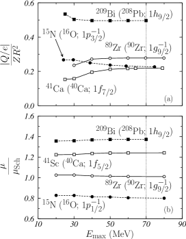
Figure 2: Convergence test of the stability of our results against $E_{\rm max}$, the upper limits of the sum on $\nu$ in Eq. (II), for $Q$, panel (a), and $\mu$, panel (b), as given by Eqs. (24) and (31), respectively. The vertical lines indicate the 70 MeV values which we have adopted as the value of $E_{\rm max}$ in our calculations.

IV Results

We have applied the model presented in the previous sections to various nuclei in different regions of the nuclear chart. The core nuclei have been selected to have closed shells and spherical symmetry, therefore, in these nuclei, deformation and pairing effects do not play any role del10 ; ang14 . We have identified isotopes of oxygen, calcium, zirconium, tin and lead endowed with these characteristics. We have investigated the role of the pairing in these nuclei by carrying out calculations in a HF plus Bardeen Cooper and Schrieffer framework ang14 . The protons and neutrons energy gaps between particle and hole states are so large that we did not find pairing effects. We found only one exception, the case of the protons in ⁹⁰Zr, where the particle fluctuation number is not exactly zero. The evaluation of the occupation probabilities of the single particle levels indicates deviations of few percent from that predicted by a sharp Fermi distribution. Only the proton $2p_{1/2}$ state, which in IPM does not contributes to the $Q$, is sensitively affected by the pairing with an occupation probability of 85%. This s.p. state does not contributes to the $Q$.

We first present the results obtained for $Q$, and, in a second step, those related to $\mu$.

IV.1 The $2^{+}$ excitations and the $Q$ values.

We show in Table 1 the excitation energies and the B(E2)$\uparrow$ values of the first $2^{+}$ state obtained in our RPA calculations for the various nuclei studied, and we compare them with the available experimental values taken from the compilations of Refs. led78 ; bnlw ; ram01 . We notice a large difference between the RPA values and the experimental ones in ¹⁶O and ⁴⁰Ca nuclei. The experimental energies are smaller than those predicted by our calculations, and the experimental B(E2)$\uparrow$ values much larger, especially in ⁴⁰Ca. Evidently, for ¹⁶O and ⁴⁰Ca, the lowest $2^{+}$ states cannot be properly described by the RPA approach since their structure is more complex than a simple combination of one-particle one-hole excitations. In effect, the experimental excitation spectrum of ¹⁶O presents at least other six 2⁺ states up to 15 MeV, and that of ⁴⁰Ca about fifty of them below 10 MeV led78 ; bnlw .

The situation for the other nuclei is different. We found reasonable agreement with the available empirical data in ⁴⁸Ca, ¹³²Sn and ²⁰⁸Pb. The 2⁺ states in these nuclei are dominated by particle-hole (ph) transitions between bound s.p. states. The simplest case is that of the ⁴⁸Ca nucleus where we found that the neutron ($2p_{3/2}\,1f_{7/2}^{-1}$) transition is the dominant component of the first $2^{+}$ excited state. We identify analogous situations in ¹³²Sn, with the proton ($2d_{5/2}\,1g_{9/2}^{-1}$) and neutron ($2f_{7/2}\,1h_{11/2}^{-1}$) transitions, and in ²⁰⁸Pb with the proton ($2f_{7/2}\,1h_{11/2}^{-1}$) and ($1h_{9/2}\,1h_{11/2}^{-1}$) and neutron ($2g_{9/2}\,1i_{13/2}^{-1}$) transitions. In these nuclei, the $2^{+}$ strength is concentrated in the s.p. transitions above mentioned with little fragmentation produced by the coupling with the continuum and/or with more complex excitations modes.

		$\omega$ (MeV)				B(E2)$\uparrow$ (e${}^{2}\,$fm4)
nucleus		D1M	D1S	exp		D1M	D1S	exp
16O		17.61	18.13	6.92		16.76	22.85	40.64
22O		2.34	2.65	3.19		15.84	14.72	28.12
24O		4.10	3.97			4.95	4.50
40Ca		13.41	14.63	3.90		3.08	3.66	99.17
48Ca		3.80	4.04	3.83		91.65	87.91	95.32
60Ca		5.82	5.63			0.39	0.40
90Zr		4.67	4.95	2.19		353.5	350.4	610.4
100Sn		4.13	4.40			1950	2055
132Sn		4.26	5.08	4.04		1574	1444
208Pb		4.91	5.05	4.09		4083	4244	3003

Table 1: Excitation energies, $\omega$ and B(E2)$\uparrow$ values of the lowest 2⁺ state for the core nuclei considered. The results obtained with the two interactions we have adopted are shown. The experimental values are taken from Refs. led78 ; bnlw ; ram01 .

core	nucleus	s.p. state	D1M	D1S	core	nucleus	s.p. state	D1M	D1S
16O	15N	$1p_{3/2}^{-1}$	2.07	2.17	100Sn	99In	$1g_{9/2}^{-1}$	22.48	23.03
	17F	$1d_{5/2}$	-4.50	-4.74		101Sb	$1g_{7/2}$	-25.04	-25.32
	17O	$1d_{5/2}$	-1.61	-1.55		99Sn	$1g_{9/2}^{-1}$	16.21	16.31
22O	21N	$1p_{3/2}^{-1}$	3.69	3.55		101Sn	$1g_{7/2}$	-19.12	-18.95
	23F	$1d_{5/2}$	-6.53	-6.35	132Sn	131In	$1g_{9/2}^{-1}$	18.61	17.70
24O	23N	$1p_{3/2}^{-1}$	2.34	2.47		133Sb	$1g_{7/2}$	-20.13	-23.02
	25F	$1d_{5/2}$	-4.58	-4.82		131Sn	$1h_{11/2}^{-1}$	14.65	12.41
40Ca	39K	$1d_{3/2}^{-1}$	4.33	4.51		133Sn	$1h_{9/2}$	-16.45	-13.45
	39Ka	$1d_{5/2}^{-1}$	5.51	5.75	208Pb	207Tl	$2d_{3/2}^{-1}$	11.33	11.93
	41Sc	$1f_{7/2}$	-8.30	-8.78		207Tla	$1h_{11/2}^{-1}$	25.62	27.08
	41Sca	$1f_{5/2}$	-10.80	-10.36		207Tlb	$2d_{5/2}^{-1}$	15.59	16.45
	39Ca	$1d_{3/2}^{-1}$	2.20	2.23		209Bi	$1h_{9/2}$	-27.71	-29.11
	41Ca	$1f_{7/2}$	-3.68	-3.66		209Bia	$2f_{7/2}$	-21.31	-22.28
48Ca	47K	$1d_{3/2}^{-1}$	5.90	5.97		209Bib	$1i_{13/2}$	-29.27	-30.79
	47Ka	$1d_{5/2}^{-1}$	7.34	7.43		207Pb	$2f_{5/2}^{-1}$	11.62	11.40
	49Sc	$1f_{7/2}$	-10.32	-10.45		207Pba	$3p_{3/2}^{-1}$	7.49	7.37
	49Sca	$1f_{5/2}$	-10.52	-10.63		207Pbb	$1i_{13/2}^{-1}$	18.54	18.58
	47Ca	$1f_{7/2}^{-1}$	4.95	4.86		207Pbc	$2f_{7/2}^{-1}$	12.97	12.80
	49Ca	$2p_{3/2}$	-2.58	-2.40		207Pbd	$1h_{9/2}^{-1}$	19.53	19.80
60Ca	59K	$1d_{3/2}^{-1}$	4.28	4.61		209Pb	$2g_{9/2}$	-14.42	-13.93
	59Ka	$1d_{5/2}^{-1}$	5.67	6.08		207Pb	$2f_{5/2}^{-1}$	11.62	11.40
	61Sc	$1f_{7/2}$	-8.17	-8.70		209Pba	$1i_{11/2}$	-21.80	-21.58
	61Sca	$1f_{5/2}$	-7.63	-8.16		209Pbb	$1j_{15/2}$	-20.11	-19.81
90Zr	91Nb	$1g_{9/2}$	-15.55	-15.94
	89Zr	$1g_{9/2}^{-1}$	8.04	8.01
	91Zr	$1g_{7/2}$	-8.62	-8.48

Table 2: Values of $Q_{\rm RPA}$, in e fm², obtained in our model for the two interactions considered. We present the core nuclei, the associated $A\pm 1$ nuclei and the s.p. states which characterize them. The upper latin letters indicate the excited states of the isotope.

The role of the continuum in this type of calculations has been studied in Ref. don11a where a detailed discussion about the position of the centroid energies and the sum rule exhaustion of the $2^{+}$ strength distribution is presented, resulting compatible with the theoretical expectations lan64 . There is a difference between the results of Ref. don11a and those of the present work, since in these latter RPA calculations the spin-orbit and Coulomb terms of the effective nucleon-nucleon interaction have been considered by using the procedure of Ref. don14a . We have verified that for the $Q$ values, and also for those of $\mu$, the differences between the two types of calculations are of the order of few percents.

If we neglect the cases of the ¹⁶O and ⁴⁰Ca nuclei, the average relative difference between our excitation energies and the experimental ones is about 15%. Even though our RPA description of the low-lying $2^{+}$ excitation of the core nuclei is not satisfactory, we have to consider that, in the calculation of $Q$ in the odd-even nearby nuclei, the relevant quantity to be considered is the global strength distribution. Our RPA calculations generate the expected amount of $2^{+}$ strength, but it is not properly distributed. This may affect our $Q$ results because the energy denominators of the kernels (10) and (11) indicate that the low-lying excited states are more important than those with high energies in the evaluation of the matrix element in Eq. (II). We have tested this sensitivity by artificially changing of the 10% the values of the $\omega_{\nu}$ energies calculated with the D1M force. The largest deviations of the $Q$ values we have identified are of about 10%, much smaller in any case than the differences with the IPM values.

Around the core nuclei, listed in Table 1, we have selected 48 states of several isotopes and isotones with one nucleon more or less, which allow us to compare our results with the experimental data of the compilation of Ref. sto05 and also with the results of Ref. rin73 obtained within the FFS theory.

In Table 2, we show the RPA results obtained in our model by using the D1M and D1S nucleon-nucleon effective interactions. In this table we indicate the core nuclei, the specific isotopes for which $Q$ was calculated, and the s.p. states characterizing them. In general, we have considered the states with lowest energy and $Q\not=0$. For example, the true ground states of ²⁰⁷Tl and ²⁰⁷Pb are a 1/2⁺ and a 1/2^- states respectively, but both have $Q=0$. For this reason, in these two cases, we have indicated the 3/2⁺ and 5/2^- states, respectively. In the table, the states of the same isotope with higher energy are indicated by a superscript latin letter.

Our calculations confirm the well known fact that the $Q$ values of nuclei with one nucleon more than the doubly closed shell core are negative, and those with a nucleon less are positive boh69 . A first general remark about the results of Table 2, is that the values we have obtained by using the two different interactions are very similar. The average relative difference between the RPA results calculated with D1M and D1S interactions is of few percent. Henceforth, if not explicitly stated, we shall discuss only the results obtained with the D1M interaction.

We compare in Fig. 3 the results of the IPM, triangles, FOPT, squares, and RPA, circles, calculations. The four panels show separately the results obtained for hole and particle-like states and for protons and neutrons. Since we do not use effective charge, the IPM results for the neutron states are zero.

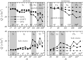
Figure 3: Values of $Q$, in e fm², for RPA (circles), FOPT (squares), and IPM (triangles), calculated with the D1M interaction for the various nuclei studied. The left (right) panels correspond to proton (neutron) states, while the upper (lower) panels show the results for particle (hole) states. The lines have been drawn to guide the eyes. The latin upper indexes indicate excited states following the nomenclature of Table 2. The RPA values for the nuclei around the ¹¹⁶Sn core, drawn as open circles, have been multiplied by 0.25.

A first, general, remark is that, in absolute value, the RPA results are always larger than those obtained in the other calculations. It is interesting to observe that, in the proton case, the FOPT results are very close to those of the IPM, and, sometime, even smaller in absolute value. In general, the RPA results produce a relatively small correction with respect to the IPM values.

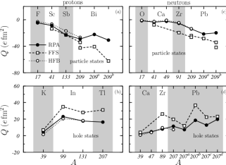
Figure 4: Values of $Q$, in $e$ fm², obtained in our RPA calculations with D1S interaction (solid circles), compared to the FFS results taken from Refs. spe77 ; tol11 ; tol12 ; voi12 (open squares) and to the HFB results found for D1S interaction (open circles).

We carried out an additional test of our model by comparing our results with those of other theoretical approaches, the Hartree-Fock-Bogolioubov (HFB) and the FFS theory spe77 ; tol11 ; tol12 ; voi12 . This comparison is shown in Fig. 4. The HFB calculations have been performed by using the technique developed by Robledo et al. rob12 , based on the gradient method. In the minimization procedure both time-even and time-odd fields are considered in the calculation of the energy functional and this allows us to avoid the equal filling approximation rod11 . In the figure, we show the RPA and HFB results obtained with the D1S interaction. The relevant point for the present study is the remarkable agreement between the HFB and our RPA results.

The other comparison proposed in Fig. 4 is that with the results of FFS calculations. This last approach is rather similar to ours, and the differences are due to the use of different interactions, and s.p. bases. The results of the nuclei around ²⁰⁸Pb taken from Ref. spe77 , have been obtained by fully exploiting the philosophy of the Landau-Migdal approach. The s.p. wave functions have been generated by using a Woods-Saxon potential well, and the RPA calculations have been conducted with a Landau-Migdal interaction whose parameters have been chosen to reproduce at best the data. The results of nuclei lighter than ²⁰⁸Pb, are taken from Refs. tol11 ; tol12 ; voi12 , and have been obtained by using a slightly different computational scheme. Skyrme interactions of different type have been used in HF calculations to generate the s.p. basis wave functions and, in the second step, also to solve the RPA equations. The zero-range characteristics of this type of interaction requires the use of a cutoff renormalisation parameter whose value depends on the size of the s.p. configuration space used in the RPA calculations. The $Q$ values obtained with the FFS approach are, in absolute value, larger than ours.

						exp
core	nucleus	s.p. state	IPM	FOPT	RPA	Ref. sto05	Ref. gar15
16O	17F	$1d_{5/2}$	-4.12	-3.74	-4.50	-5.80
	17O	$1d_{5/2}$	0.0	-1.51	-1.61	-2.60
40Ca	39K	$1d^{-1}_{3/2}$	3.37	3.04	4.33	5.90
	41Sc	$1f_{7/2}$	-7.01	-6.31	-8.30	-15.60
	39Ca	$1d^{-1}_{3/2}$	0.0	1.78	2.20	3.60
	41Ca	$1f_{7/2}$	0.0	-3.17	-3.68	-9.00
48Ca	47Ca	$1f^{-1}_{7/2}$	0.0	2.43	4.95	2.10	8.46
	49Ca	$2p_{3/2}$	0.0	-1.24	-2.58		-3.63
90Zr	91Zr	$2d_{5/2}$	0.0	-3.15	-5.68	-17.60
208Pb	209Bi	$1h_{9/2}$	-16.39	-13.84	-27.71	-51.60
	209Pb	$2g_{9/2}$	0.0	-7.55	-14.42	-30.00

Table 3: Values of $Q$, in e fm², for IPM, FOPT and RPA, calculated with the D1M interaction, compared to the experimental data taken from the compilation sto05 and from Ref. gar15 . The s.p. states refer to the corresponding doubly magic cores.

In Table 3 we compare our results with the experimental values taken from the compilation of Ref. sto05 and with those given in Ref. gar15 . The RPA description of these experimental data is not particularly satisfactory. All the experimental values are larger than our predictions. In heavier nuclei our calculations are able to account only for about half of the observed $Q$ values. This indicates that our approach is not fully able to describe the large collectivity of the $2^{+}$ excitations. On the other hand, the improvement with respect to the IPM predictions, and also with respect to the FOPT predictions, is remarkable.

IV.2 The $\mu$ and the $1^{+}$ excitation.

We use the same set of even-even core nuclei adopted for the calculation of $Q$ also for the investigation of the magnetic dipole moment $\mu$. Around each core nucleus we calculate the $\mu$ values for the four nuclei with one nucleon more or less. We present our results by following the strategy adopted in the investigation of $Q$. We first discuss the features of the $1^{+}$ excitation in the core nuclei and, after, we present the results of the calculation of $\mu$ and we compare them with the experimental values.

We present in Table 4 the excitation energies and the B(M1)$\uparrow$ values of the main low-lying $1^{+}$ states, and we compare them with the experimental values taken from Refs. led78 ; bnlw . We indicate in the table also the dominant ph transitions.

		$\omega$ (MeV)				B(M1)$\uparrow$ ($\mu_{N}^{2}$)			main s.p. transitions
nucleus		D1M	D1S	exp		D1M	D1S		proton	neutron
16O		17.76	18.37	13.66		0.01	0.01		$(2p_{3/2}1p^{-1}_{1/2})$
22O		8.35	8.97			5.81	5.18			$(1d_{3/2}1d^{-1}_{5/2})$
24O		8.50	9.06	9.50		5.75	5.13			$(1d_{3/2}1d^{-1}_{5/2})$
40Ca		14.62	15.03	9.87		0.006	0.006		$(2d_{5/2}1d^{-1}_{3/2})$
48Ca		9.30	10.19	10.23		10.23	9.66			$(1f_{5/2}1f^{-1}_{7/2})$
60Ca		6.73	6.76			0.04	0.04			$(3p_{3/2}2p^{-1}_{1/2})$
90Zr		9.08	9.98	9.37		13.98	13.49			$(1g_{7/2}1g^{-1}_{9/2})$
100Sn		7.49	9.13			0.65	0.97		$(1f_{5/2}1f^{-1}_{7/2})$
132Sn		6.78	8.00			6.05	9.84		$(1f_{5/2}1f^{-1}_{7/2})$
208Pb		6.30	7.60	5.85		7.80	11.89		$(1i_{11/2}1i^{-1}_{13/2})$	$(1h_{9/2}1h^{-1}_{11/2})$

Table 4: Energies, $\omega$, and B(M1)$\uparrow$ values of the main low-lying $1^{+}$ excited state obtained in our calculations for the core nuclei considered, with the two interactions we have adopted. The experimental values are taken from Refs. led78 ; bnlw .

The table shows that the B(M1)$\uparrow$ values of the ¹⁶O, ⁴⁰Ca and ⁶⁰Ca nuclei, where all the spin-orbit partner levels are occupied, are orders of magnitudes smaller than the other ones. This confirms the well known fact boh69 ; ram91 that the M1 excitation is strongly excited in nuclei where ph transitions between spin-orbit partner levels are allowed. We have presented in Ref. co12b a detailed discussion of the M1 strength distribution in oxygen and calcium isotopes.

The agreement with the experimental energies is reasonable for almost all the cases, but for ¹⁶O and ⁴⁰Ca. We have already pointed out the fact that in the first two nuclei the $1^{+}$ excitation is rather weak because all the spin-orbit partner levels are occupied. In these nuclei it is not easy to find out the $1^{+}$ states to be compared with those predicted by our model, since, experimentally, the M1 strength is rather fragmented. For example in ⁴⁰Ca we found more than twenty $1^{+}$ states below 12 MeV led78 ; bnlw .

Our description of the $1^{+}$ excitation is rather good in the situations where these excitations are dominated by a few ph transitions. In these cases our approach works at its best. The main features of the transitions are already well described within the IPM which is corrected by the RPA by including other, less important, ph transitions.

The ten doubly magic nuclei listed in Table 4 have been considered as core nuclei where we add or remove one nucleon at the time to form odd-even nuclei with magnetic dipole moment $\mu$. Before discussing the effects of the core polarization, i.e. of the excitation of the even-even core, we clarify the role played by the MEC in the calculation of $\mu$.

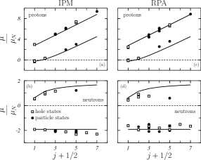
Figure 5: Comparison between the values of $\mu_{\rm IPM}$, left panels, and $\mu_{\rm RPA}$, right panels, expressed in nuclear magnetons, and the Schmidt values, as a function of the angular momentum $j$ of the odd-even nucleus. The results obtained with the full electromagnetic operator, ${\cal M}_{1}={\cal M}_{1}^{\rm OB}+{\cal M}_{1}^{\rm MEC}$, are indicated by the symbols and the Schmidt values by the solid lines. Open squares and solid circles represent the results obtained, respectively, for nuclei characterized by hole or particle-like s.p. states. The calculations have been carried out with the D1M interaction.

In Fig. 5 we adopt the usual representation of $\mu$ rin80 against the angular momentum $j$ of the odd-even nucleus, to show our results obtained with the D1M force. In the (a) and (b) panels the symbols represent the $\mu_{\rm IPM}$ values obtained by considering the full electromagnetic operator ${\cal M}_{1}={\cal M}_{1}^{\rm OB}+{\cal M}_{1}^{\rm MEC}$, while the lines indicate the Schmidt values found for ${\cal M}_{1}^{\rm OB}$ (see Eq. (32)). The MEC produce relatively small changes with respect to the Schmidt values, usually of the order of few percent up to a maximum value of about $10\%$. These changes have a consistent behavior over all the various regions of the nuclear chart, and we did not observe remarkable differences between nuclei characterized by a hole- (open squares) or a particle-like (solid circles) structure.

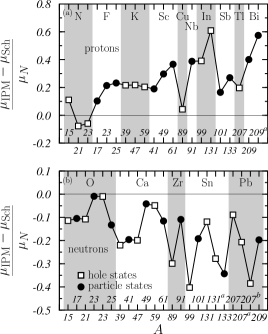
Figure 6: Difference $\mu_{\rm IPM}-\mu_{\rm Sch}$, expressed in nuclear magnetons, for proton, panel (a), and neutron, panel (b), odd nuclei. Open squares and solid circles represent the results obtained for nuclei characterized by hole or particle-like structure. The calculations have been carried out with the D1M interaction.

Another perspective to observe these results is given in Fig. 6 where we show the differences $\mu_{\rm IPM}-\mu_{\rm Sch}$ as a function of the mass number of the nuclei investigated. The results of panel (a) correspond to the odd-proton nuclei while those of panel (b) are those obtained for the odd-neutron nuclei. In the odd-proton cases the MEC always increase the $\mu$ values with respect to the Schmidt ones, but for the ²¹N and ²³N nuclei. The results of panel (b) show that the effect of the MEC on the odd-neutron nuclei consists in a lowering with respect to the Schmidt values, without exceptions. It is possible to outline a general overall tendency of the MEC effects to increase with the mass number, even though there are quite a few exceptions.

The effects we have just described are consistent for all the nuclei, and, in terms of the agreement with the experimental data implies two contrasting aspects. Since the experimental data are lying between the two Schmidt lines, the inclusion of the MEC improves the agreement for odd-proton nuclei with $j_{<}\equiv l-1/2$, while they are worsening it for odd-proton nuclei with $j_{>}\equiv l+1/2$. We have a similar situation also for the odd-neutron nuclei where we observe an improvement in the case of $j_{<}$ and a worsening for $j_{>}$.

core	nucleus	s.p. state	D1M	D1S		core	nucleus	s.p. state	D1M	D1S
16O	15N	1p${}_{1/2}^{-1}$	-0.137	-0.142		90Zr	89Y	2p${}_{1/2}^{-1}$	-0.108	-0.152
	17F	1d5/2	4.884	4.885			91Nb	1g9/2	6.727	6.996
	15O	1p${}_{1/2}^{-1}$	0.638	0.638			89Zr	1g${}_{9/2}^{-1}$	-1.937	-1.813
	17O	1d5/2	-2.088	-2.007			91Zr	2d5/2	-1.808	-1.715
22O	21N	1p${}_{1/2}^{-1}$	0.001	-0.042		100Sn	99In	1g${}_{9/2}^{-1}$	6.559	6.593
	23F	1d5/2	4.397	4.779			101Sb	2d5/2	4.448	4.476
	21O	1d${}_{5/2}^{-1}$	-1.667	-1.487			99Sn	1g${}_{9/2}^{-1}$	-1.638	-1.771
	23O	2s1/2	-1.610	-1.485			101Sn	2d5/2	-1.507	-1.614
24O	23N	1p${}_{1/2}^{-1}$	0.013	-0.024		132Sn	131In	1g${}_{9/2}^{-1}$	6.788	6.767
	25F	1d5/2	4.444	4.801			133Sb	1g7/2	2.579	2.546
	23O	2s${}_{1/2}^{-1}$	-1.628	-1.482			131Sn	2d${}_{3/2}^{-1}$	0.684	0.758
	25O	1d3/2	0.842	0.841			131Sna	1h${}_{11/2}^{-1}$	-1.520	-1.688
40Ca	39K	1d${}_{3/2}^{-1}$	0.358	0.350			133Sn	1h9/2	0.596	0.746
	41Sc	1f7/2	5.971	5.972		208Pb	207Tl	3s${}_{1/2}^{-1}$	2.528	2.538
	39Ca	1d${}_{3/2}^{-1}$	0.910	0.918			209Bi	1h9/2	3.604	3.548
	41Ca	1f7/2	-2.096	-2.098			209Bia	1i13/2	8.859
48Ca	47K	2s${}_{1/2}^{-1}$	2.384	2.695			207Pb	3p${}_{1/2}^{-1}$	0.437	0.463
	49Sc	1f7/2	5.577	5.888			207Pba	2f${}_{5/2}^{-1}$	0.764	0.857
	47Ca	1f${}_{7/2}^{-1}$	-1.809	-1.664			207Pbb	1i${}_{13/2}^{-1}$	-1.655
	49Ca	2p3/2	-1.709	-1.605			209Pb	2g9/2	-1.635	-1.756
60Ca	59K	1d${}_{3/2}^{-1}$	0.347	0.338
	61Sc	1f7/2	6.146	6.147
	59Ca	2p${}_{3/2}^{-1}$	-1.954	-1.951
	61Ca	1g9/2	-2.015	-2.011

Table 5: Values of $\mu$, in nuclear magnetons, obtained in our RPA model with the full ${\cal M}_{1}^{\rm\,OB}+{\cal M}_{1}^{\rm\,MEC}$ operator for the two interactions considered. We present the core nuclei, the specific $A\pm 1$ nuclei and the s.p. states which characterise them. The upper latin letters indicate the excited states of the isotope.

In Table 5 we present the RPA results obtained with the two interactions we have adopted, and by using the full electromagnetic operator which includes the MEC. We have considered those configurations which generate the ground state of the odd-even nuclei, and some excited state of interest. In the table, our results are compared to the available data taken from the compilation of Ref. sto05 .

With the exceptions of the ²¹N, ²³N, and ¹³¹Sn cases, some of which we shall discuss in more detail, the relative differences between the D1M and D1S results are of the order of 1%. This indicates that the effects we are discussing are almost independent of the specific implementation of the interaction used.

The quantitative stability of our results can be observed by considering that, in our approach, the ²³O nucleus can be obtained by adding a neutron to the ²²O core or subtracting one to ²⁴O. The differences between the two procedures are related to the different s.p. states produced by the HF calculations and the results obtained for D1M and D1S interactions show $\mu$ values that differ on the third and fourth significant figures, respectively.

We compare the D1M results of Table 5 with the Schmidt values in the panels (c) and (d) of Fig. 5. In general, the $\mu_{\rm RPA}$ values are situated between the two Schmidt lines, as it is observed for the experimental values. The deviation from the Schmidt values is particularly evident in the neutron case for the nuclei with $j_{<}$ above 5/2, which correspond to the ²⁰⁷Pb^a and ¹³³Sn isotopes.

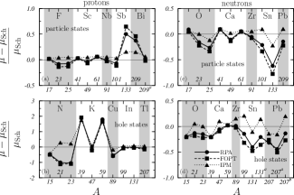
Figure 7: Comparison between our RPA, circles, FOPT, squares, and IPM, triangles, results. The calculations have been carried out with the D1M interaction and by using the full electromagnetic operator ${\cal M}_{1}={\cal M}_{1}^{\rm OB}+{\cal M}_{1}^{\rm MEC}$. The lines have been drawn to guide the eyes.

In Fig. 7 we compare the RPA, FOPT and IPM results. All the calculations have been carried out with the D1M interaction, and by using the complete electromagnetic operator ${\cal M}_{1}={\cal M}_{1}^{\rm OB}+{\cal M}_{1}^{\rm MEC}$. The results are shown as relative difference with respect to the Schmidt values, Eq. (32). We observe the great similarity between our RPA results and those obtained in FOPT. This indicates that the structure of the $1^{+}$ states is not as collective as that of the $2^{+}$ states, but it is rather dominated by single-particle excitations.

The FOPT and RPA results show very similar behaviors. In general, the FOPT deviate more from the Schmidt values than the RPA ones. We remark that the FOPT approach, often utilized in the literature bli53 ; ari54 ; ari11 ; li11 ; li13 , performs much better in this case than for the electric quadrupole moment case, as it is shown in Fig. 4.

Our results agree with those of the non-relativistic calculations of Refs. li13 ; ari11 . More precisely, and always with respect to the Schmidt values, we observe that: (i) both MEC and RPA increase the $\mu$ values in ²⁰⁹Bi; (ii) in ²⁰⁷Tl we find an enhancement due to the MEC while the RPA effects produce a lowering of $\mu$; (iii) in ²⁰⁹Pb we have opposite effects, and (iv) in ²⁰⁷Pb both MEC and RPA lower the $\mu$ values.

The $\mu$ values obtained in RPA show a remarkable difference with respect to the IPM results. The case of the ³⁹K and ⁵⁹K nuclei is particularly interesting since the three calculations provide very similar results and all of them noticeably deviate from the Schmidt values. This is only due to the presence of MEC in the operator. This effect should be investigated better, by considering also that the ⁴⁷K nucleus does not present this feature.

core	nucleus	s.p. state	Schmidt	IPM	FOPT	RPA	FFS	exp
16O	15N	1p${}_{1/2}^{-1}$	-0.264	-0.153	-0.133	-0.137	—	-0.283
	17F	1d5/2	4.793	4.896	4.882	4.884	—	4.721
	15O	1p${}_{1/2}^{-1}$	0.638	0.524	0.506	0.510	—	0.720
	17O	1d5/2	-1.913	-2.018	-2.003	-2.088	—	-1.894
40Ca	39K	1d${}_{3/2}^{-1}$	0.124	0.340	0.361	0.358	0.329	0.391
	41Sc	1f7/2	5.793	5.983	5.963	5.971	5.485	5.431
	39Ca	1d${}_{3/2}^{-1}$	1.148	0.928	0.910	0.910	0.888	1.022
	41Ca	1f7/2	-1.913	-2.109	-2.088	-2.096	-1.626	-1.595
48Ca	47K	2s${}_{1/2}^{-1}$	2.793	3.011	2.173	2.384	—	1.933
	47Ca	1f${}_{7/2}^{-1}$	-1.913	-2.112	-1.732	-1.809	-1.556	-1.380
	49Ca	2p3/2	-1.913	-1.954	-1.654	-1.709	-1.156	—
90Zr	89Y	2p${}_{1/2}^{-1}$	-0.264	-0.221	-0.114	-0.108	-0.125	-0.137
	89Zr	1g${}_{9/2}^{-1}$	-1.913	-2.212	-1.872	-1.937	-1.304	-1.046
	91Zr	2d5/2	-1.913	-2.022	-1.769	-1.808	-1.214	-1.304
132Sn	133Sb	1g7/2	1.717	1.987	2.826	2.579	2.693	3.000
	131Sn	2d${}_{3/2}^{-1}$	1.148	1.029	0.601	0.684	0.681	0.747
	131Sna	1h${}_{11/2}^{-1}$	-1.913	-2.191	-1.227	-1.520	—	-1.276
208Pb	207Tl	3s${}_{1/2}^{-1}$	2.793	2.990	2.379	2.528	1.857	1.876
	209Bi	1h9/2	2.624	3.025	3.827	3.604	3.691	4.110
	207Pb	3p${}_{1/2}^{-1}$	0.638	0.549	0.472	0.437	0.473	0.593
	207Pba	2f${}_{5/2}^{-1}$	1.366	1.159	0.677	0.764	0.720	0.800
	209Pb	2g9/2	-1.913	-2.110	-1.486	-1.635	-1.337	-1.474

Table 6: Comparison between $\mu$ values, expressed in nuclear magnetons, calculated in IPM, FOPT and RPA by using the complete electromagnetic operator ${\cal M}_{1}^{\rm\,OB}+{\cal M}_{1}^{\rm\,MEC}$ with the Schmidt values (32), the FFS results of Ref. bor08 and the experimental data of Ref. sto05 .

A direct comparison between our results and the available experimental data taken from Ref. sto05 is presented in Table 6. In this table we also include the results of the FFS calculation of Ref. bor08 . We observe that the effects of the core polarisation become more important in the heavier nuclei. The differences between the results of IPM, FOPT and RPA calculations are rather small in the nuclei around ¹⁶O and ⁴⁰Ca.

In the great majority of the cases the RPA results are closer to the experimental values than the other ones, indicating that the inclusion of the core polarization improves the agreement with the available experimental data. However, this is not a universal behavior since there are very specific cases, where the IPM approach produce a better description of the observed $\mu$ values. As expected the FFS results, which use effective electromagnetic operators, are in general closer to the experimental values that ours.

nucleus	interaction	Schmidt	IPM	FOPT	RPA
21N	D1M	-0.264	-0.341	0.030	0.001
	D1S	-0.264	-0.339	0.003	-0.042
23N	D1M	-0.264	-0.323	0.025	0.013
	D1S	-0.264	-0.322	-0.002	-0.024

Table 7: Values of $\mu$, in nuclear magnetons, of the ²¹N and ²³N nuclei. The Schmidt values are compared to those found within IPM, FOPT and RPA approaches with the full ${\cal M}_{1}^{\rm\,OB}+{\cal M}_{1}^{\rm\,MEC}$ operator.

We conclude this section by analyzing in detail the cases of the ²¹N and ²³N nuclei. In Table 7 we show the $\mu$ values for these two nuclei calculated by using different approximations. We observe that the Schmidt values have negative sign. The inclusion of the MEC in the IPM calculations gives a negative contribution, further lowering these values. The core polarization plays an important role as the results of two last columns indicate. In both nuclei, the effect of the residual interaction has opposite sign with respect to the contribution of the MEC. This effect is larger in the FOPT than in RPA results. In RPA calculations, the effects of the D1M force are large enough to change the sign of $\mu$ with respect to the Schmidt value. Experimental $\mu$ values for these two nuclei are not available. In any case, our RPA results follow the trend of the know experimental values of lying between the Schmidt values.

V Conclusions

In this work, we have presented the results of a parameter free theoretical approach which describes the properties of odd-even nuclei with one nucleon more, or less, than a doubly magic one. The convergence of the energy sum in Eq. (II), the fundamental equation of our model, is ensured by the use of finite-range nucleon-nucleon effective interaction. The use of zero-range interactions, as it is done for example in Refs. rin73 ; bau73 ; spe77 , requires the inclusion of additional free parameters. The universality of our approach allows us to apply it in each region of the nuclear chart, from light to heavy nuclei.

We have considered two parameterizations of the finite-range effective Gogny nucleon-nucleon interaction taken from the literature, the D1S and D1M. Our calculations are fully self-consistent, meaning that all results have been obtained by using the same interaction in each of the three steps of the calculation: the generation of the s.p. configuration space by means of a HF procedure, the solution of the RPA equations and, finally, the evaluation of the response of the odd-even nucleus to the external probe. In each step of the calculation the complete interaction has been used, including the spin-orbit and the Coulomb terms, commonly neglected in RPA.

We have tested the validity of our approach by calculating the values of the electric quadrupole moment, $Q$, of 48 different states, and the magnetic dipole moment, $\mu$, of 44 states, in various regions of the nuclear chart. We have used the traditional one-body operator for the calculation of $Q$, while for the $\mu$ we have considered also the contribution of MEC. We use bare electromagnetic operators whose coupling constants are those of free nucleons.

In absolute value, the results obtained by considering the MEC are always larger than the Schmidt values, implying an improvement of the agreement with experimental data for odd-proton nuclei with $j_{<}$ and with odd-neutron nuclei with $j_{>}$, and a worsening for the other type of nuclei.

The differences between the results obtained with the two forces are small, negligible if compared to the differences between RPA and IPM results. This indicates that the quantitative description of the core polarisation effects in our calculations is more related to the theoretical approach, rather than to the use of a specific interaction.

Our calculations require the description of the excitation of $2^{+}$ and $1^{+}$ states in doubly closed shell nuclei, in the framework of the RPA theory. We observe that our model describe better the $1^{+}$ excitations than the $2^{+}$ ones. This occurs because the most important $1^{+}$ states, those where the largest part of the strength is concentrated, are dominated by a single ph transition. In this case, our approach works at its best, by correcting the main ph transition with the presence of other one-particle one-hole transitions. On the other hand, the structure of many of the $2^{+}$ states is very collective, and a good description of it requires to go beyond the linear combination of one-particle one-hole transitions which is what the RPA considers.

This difference in the description of the two multipolarities is reflected in the results we have obtained for the values of $Q$ and $\mu$. The description of the magnetic dipole moments is certainly better than that of the electric quadrupole moments. The similarity between our results and those obtained in FOPT is a further indication of the perturbative structure of the $1^{+}$ excitations. In any case, we have to point out that our results show a remarkable improvement of the description of the experimental values with respect to the IPM predictions, and also with respect to the FOPT for $Q$.

We found a good agreement between our results and those of the FFS theory given in the literature rin73 ; bau73 ; spe77 ; bor08 ; bor10 ; tol11 ; tol12 ; voi12 . The basic theoretical hypotheses of the two approaches are rather similar. More remarkable is the agreement with the $Q$ values obtained in the HFB calculations. Our approach and the HFB treat the core polarisation in a completely different manner, but they produce similar results. In our approach the IPM response is corrected by the core polarisation described in terms of particle-hole excitations. Alternatively the HFB theory corrects the IPM by considering the effects of the pairing force. These two alternative visions of effects beyond the IPM picture generate very similar quantitative results. It would be interesting to identify specific observables which allow us to disentangle the two effects.

Despite the limitations we have pointed out, we think that our parameter free, self-consistent approach is adequate to make predictions of the properties of odd-even nuclei nearby the doubly magic-ones in regions of the nuclear chart not yet experimentally explored.

Appendix A MEC matrix elements

In this appendix we give the explicit expressions of the matrix elements of the MEC inserted in Eq. (II) to calculate the values of $\mu$. We have considered the contribution of the two diagrams indicated in Fig. 1 and called them seagull and pionic. We give here the final results of a calculation which describes these contributions in terms of Feynman’s diagrams, makes a non-relativistic reduction, a multipole expansion and the use of s.p. wave functions with the angular coupling indicated in Eq. (8).

We call $q$ the modulus of the momentum that the photon is exchanging with the nucleus, and $\omega$ the photon energy. In the specific case under study we have $\omega=\epsilon_{\alpha\beta}$ and $q=\omega/(\hbar c)$.

The contribution of the seagull term is given by

$$\langle\,\phi_{a}\,\|\,{\cal M}^{\rm s}_{J}\,\|\,\phi_{b}\,\rangle = \xi(l_{\alpha}+l_{\beta}+J+1)\,(-1)^{j_{a}-1/2}\,\frac{\widehat{j}_{a}\widehat{j}_{b}\widehat{J}}{\sqrt{J(J+1)}}\,\left(\begin{array}[]{ccc}j_{a}&j_{b}&J\\ \frac{1}{2}&-\frac{1}{2}&0\end{array}\right)$$

$$\times\left[G^{P}_{E}(q,\omega)\,-\,G^{N}_{E}(q,\omega)\right]\,\int{\rm d}r\,r^{2}\,j_{J}(qr)\,{\cal F}^{(\rm s)}_{a,b,J}(r)\,,$$

where $G^{P}_{E}$ and $G^{N}_{E}$ are, respectively, the proton and neutron electromagnetic form factors, and we have defined

$${\cal F}^{(\rm s)}_{a,b,J}(r) = -2\,\frac{f^{2}_{\pi}}{m^{2}_{\pi}}\,\sum_{h<\epsilon_{\rm F}}\,\widehat{j}_{h}^{2}\,\left[\delta_{ab,p}\delta_{h,n}-\delta_{ab,n}\delta_{h,p}\right]$$ (42)

$$\times\left\{\sum_{L_{1}}\xi(l_{a}+l_{h}+L_{1}+1)\,\widehat{L}^{2}_{1}\,\left(\begin{array}[]{ccc}j_{a}&j_{h}&L_{1}\\ \frac{1}{2}&-\frac{1}{2}&0\end{array}\right)^{2}\,\kappa_{ab}\,{\cal T}_{ah}(L_{1},r)\,R_{h}(r)\,R_{b}(r)\right.$$

$$\,\,\,\,\,\,\,\,\,\,\,\,+\,\left.\sum_{L_{2}}\,\xi(l_{b}+l_{h}+L_{2}+1)\,\widehat{L}^{2}_{2}\,\left(\begin{array}[]{ccc}j_{h}&j_{b}&L_{2}\\ \frac{1}{2}&-\frac{1}{2}&0\end{array}\right)^{2}\,\kappa_{ab}\,{\cal T}_{hb}(L_{2},r)\,R_{a}(r)\,R_{h}(r)\right\}\,,$$

where $f^{2}_{\pi}=0.079$ is the pion-nucleon coupling constant, $m_{\pi}$ is the pion mass, $\kappa$ is defined in Eq. (30), $\xi(l)=1$ if $l$ is even and zero otherwise, $R(r)$ is the radial part of the s.p. wave function (8), and ${\cal T}$ is defined as

$${\cal T}_{ab}(L,x) = \int_{0}^{\infty}{\rm d}r\,r^{2}\,\left\{\left(\frac{\rm d}{{\rm d}r}\,+\,\frac{\kappa_{ab}+2}{r}\right)\,R_{a}(r)\,R_{b}(r)\right\}$$ (43)

$$\times\int_{0}^{\infty}{\rm d}k\,k^{2}\,\frac{2}{\pi}\,v_{\pi}(k,\epsilon_{ab})\,j_{L}(kr)\,j_{L}(kx)\,.$$

In the above equations we have indicated with $v_{\pi}$ the pion propagator

$$v_{\pi}(k,\epsilon)\,=\,\frac{1}{k^{2}-\epsilon^{2}+m^{2}_{\pi}}\,.$$ (44)

The contribution of the pionic term is

$$\langle\,\phi_{a}\,\|\,{\cal M}^{\pi}_{J}\,\|\,\phi_{b}\,\rangle\,=\,\xi(l_{\alpha}+l_{\beta}+J+1)\,\widehat{j}_{a}\,\widehat{j}_{b}\,\widehat{J}\,F_{\pi\gamma}(q,\omega)\,\int{\rm d}r\,r^{2}\,j_{J}(qr)\,{\cal F}^{(\pi)}_{a,b,J}(r)\,,$$ (45)

where

$$F_{\pi\gamma}(q,\omega)\,=\,\frac{1}{1+(q^{2}-\omega^{2})/m_{\rho}^{2}}\,$$ (46)

is the electromagnetic form factor of the pion, with $m_{\rho}=776.0\,$MeV the $\rho$-meson mass, and

$${\cal F}^{(\pi)}_{a,b,J}(r) = 4\,\frac{f^{2}_{\pi}}{m^{2}_{\pi}}\,\frac{1}{r}\,\sum_{h<\epsilon_{\rm F}}\,(-1)^{j_{h}+j_{b}}\,\widehat{j}^{2}_{h}\,\left[\delta_{ab,p}\delta_{h,n}-\delta_{ab,n}\delta_{h,p}\right]$$

$$\times\sum_{L_{1}L_{2}}\,\xi(l_{a}+l_{h}+L_{1}+1)\,\xi(l_{b}+l_{h}+L_{2}+1)\,\widehat{L}^{2}_{1}\,\widehat{L}^{2}_{2}$$

$$\times\left\{\begin{array}[]{ccc}L_{1}&L_{2}&J\\ j_{b}&j_{a}&j_{h}\end{array}\right\}\,\left(\begin{array}[]{ccc}j_{a}&j_{h}&L_{1}\\ \frac{1}{2}&-\frac{1}{2}&0\end{array}\right)\,\left(\begin{array}[]{ccc}j_{h}&j_{b}&L_{2}\\ \frac{1}{2}&-\frac{1}{2}&0\end{array}\right)\,\left(\begin{array}[]{ccc}L_{1}&J&L_{2}\\ 1&-1&0\end{array}\right)\,$$

$$\times\sqrt{L_{2}(L_{2}+1)}\,{\cal T}_{ah}(L_{1},r)\,{\cal T}_{hb}(L_{1},r)\,.$$

- (1) P. Goode, B. J. West, S. Siegel, Nucl. Phys. A 187 (1972) 249.
- (2) P. J. Ellis, E. Osnes, Rev. Mod. Phys. 49 (1977) 777.
- (3) J. Li, J. X. Wei, J. N. Hu, P. Ring, J. Meng, Phys. Rev. C 88 (2013) 064307.
- (4) A. Migdal, Theory of finite Fermi systems and applications to atomic nuclei, Interscience, London, 1967.
- (5) P. Ring, R. Bauer, J. Speth, Nucl. Phys. A 206 (1973) 97.
- (6) R. Bauer, J. Speth, V. Klemt, E. Werner, T. Yamazaki, Nucl. Phys. A 209 (1973) 535.
- (7) J. Speth, E. Werner, W. Wild, Phys. Rep. 33 (1977) 127.
- (8) I. N. Borzov, E. E. Saperstein, S. V. Tolokonnikov, Physcs of Atomic Nuclei 71 (2008) 469.
- (9) I. N. Borzov, E. E. Saperstein, S. V. Tolokonnikov, G. Neyens, N. Severijns, Eur. Phys. J. A 45 (2010) 159.
- (10) S. V. Tolokonnikov, S. Kamerdzhiev, D. Voitenkov, S. Krewald, E. E. Saperstein, Phys. Rev. C 84 (2011) 064324.
- (11) S. V. Tolokonnikov, S. Kamerdzhiev, S. Krewald, E. E. Saperstein, D. Voitenkov, Eur. Phys. J. A 48 (2011) 70.
- (12) D. Voitenkov, O. Achakovskiy, S. Kamerdzhiev, S. V. Tolokonnikov, arxiv:1210.1691 [nucl-th].
- (13) F. Chappert, Nouvelles paramétrisation de l’interaction nucléaire effective de Gogny, Ph.D. thesis, Université de Paris-Sud XI (France), http://tel.archives-ouvertes.fr/tel-001777379/en/ (2007).
- (14) V. De Donno, G. Co’, M. Anguiano, A. M. Lallena, Phys. Rev. C 89 (2014) 014309.
- (15) A. L. Fetter, J. D. Walecka, Quantum theory of many-particle systems, McGraw-Hill, S. Francisco, 1971.
- (16) P. Ring, P. Schuck, The nuclear many-body problem, Springer, Berlin, 1980.
- (17) A. R. Edmonds, Angular momentum in quantum mechanics, Princeton University Press, Princeton, 1957.
- (18) T. Schmidt, Z. Phys. 106 (1937) 358.
- (19) A. Bohr, B. R. Mottelson, Nuclear structure, vol. I, Benjamin, New York, 1969.
- (20) J. F. Berger, M. Girod, D. Gogny, Comp. Phys. Commun. 63 (1991) 365.
- (21) S. Goriely, S. Hilaire, M. Girod, S. Péru, Phys. Rev. Lett. 102 (2009) 242501.
- (22) V. De Donno, G. Co’, M. Anguiano, A. M. Lallena, Phys. Rev. C 90 (2014) 024326.
- (23) J.-P. Delaroche, M. Girod, J. Libert, H. Goutte, S. Hilaire, S. Péru, N. Pillet, G. F. Bertsch, Phys. Rev. C 81 (2010) 014303.
- (24) M. Anguiano, A. M. Lallena, G. Co’, V. De Donno, J. Phys. G 41 (2014) 025102.
- (25) C. M. Lederer, V. S. Shirley, Table of isotopes, 7th ed., John Wiley and sons, New York, 1978.
- (26) Brookhaven National Laboratory, National nuclear data center, http://www.nndc.bnl.gov/.
- (27) S. Raman, C. W. Nestor Jr., P. Tikkanen, Phys. Rev. C 41 (1990) 1084.
- (28) V. De Donno, G. Co’, M. Anguiano, A. M. Lallena, Phys. Rev. C 83 (2011) 044324.
- (29) A. M. Lane, Nuclear theory, W. A. Benjamin, New York, 1964.
- (30) N. J. Stone, Atomic Data and Nuclear Data Tables 90 (2005) 75.
- (31) L. M. Robledo, R. Bernard, G. F. Bertsch, Phys. Rev. C 86 (2012) 064313.
- (32) R. Rodríguez-Guzmán, P. Sarriguren, L. M. Robledo, Phys. Rev. C 83 (2011) 044307.
- (33) R. F. Garcia Ruiz, et al., arxiv:1504.04474 [nucl-exp].
- (34) S. Raman, L. W. Fagg, R. S. Hicks, Giant magnetic resonances, in Electric and magnetic giant resonances in nuclei, J. Speth ed., World Scientific, Singapore, 1991.
- (35) G. Co’, V. De Donno, M. Anguiano, A. M. Lallena, Phys. Rev. C 85 (2012) 034323.
- (36) R. J. Blin-Stoyle, Proc. Phys. Soc. A 66 (1953) 1158.
- (37) A. Arima, H. Horie, Prog. Part. Nucl. Phys. 12 (1954) 623.
- (38) A. Arima, Sci. China Phys. Mec. Astron. 54 (2011) 188.
- (39) J. Li, J. M. Yao, J. Meng, A. Arima, Prog. Theor. Phys. 125 (2011) 1185.