Stability of patterns on thick curved surfaces

Abstract

We consider reaction-diffusion equations on a thick curved surface and obtain a set of effective R-D equation to ${\cal O}(\epsilon^{2})$, where $\epsilon$ is the surface thickness. We observe that the R-D systems on these curved surfaces can have space- dependent reaction kinetics. Further, we use linear stability analysis to study the Schnakenberg model on spherical and cylindrical geometries. The dependence of steady state on the thickness is determined for both cases, and we find that a change in the thickness can stabilize the unstable patterns, and vice versa. The combined effect of thickness and curvature can play an important role in the rearrangement of spatial patterns on thick curved surfaces.

I INTRODUCTION

In 1952 Turing Turing (1952) proposed the reaction-diffusion
(R-D) mechanism, where the chemicals can react and diffuse so as to produce spatially varying concentrations of chemicals in the steady state. Since then many models Murray (2001); Koch and Meinhardt (1994) have been proposed to mimic the complex pattern formation in biological systems. Turing-like R-D equations are routinely used in trying to understand the skin patterns of animals Murray (2001); for example in fish Shoji et al. (2002), mammals Bard (1981), snakes Murray and Myerscough (1991) leopards Liu et al. (2006) and many others. There have also been attempts to study changes in the pigmentation patterns on leopards and jaguars as they grow in size Liu et al. (2006).

In most studies, R-D equations are analyzed on flat geometries which are not always suitable for the study of patterns on animal skin surfaces. It is reasonable to assume that geometry of the surface can play an important role in determining the pattern formation. For instance, Turing considered the surface of a sphere in the context of gastrulation of a blastula Turing (1952). Geometry is probably responsible for stripes at the end of the tail while there are spots elsewhere in some animals Murray (2001). Understanding the pattern formation on curved surfaces can be important in some chemical, biochemical and embryological process Varea et al. (1999). It is also known that organ morphogenesis can be controlled by tissue geometry Nelson et al. (2006). Recently some studies have been initiated to understand the role of curvature in biological systems Halbedel et al. (2009); Peter et al. (2004); Gov and Gopinathan (2006); Orlandini et al. (2013).

The thickness of the surface is being neglected in most earlier studies. For instance, blastula is considered as a hollow sphere assuming no thickness Turing (1952). But protein diffusion in lipid bilayers can be viewed as a diffusion on a two-dimensional curved surface with thickness. In some of the recent studies, there has been attempts to incorporate the small thickness Ogawa (2010); Balois et al. (2014). The combined role of geometry and thickness can lead to curvature-dependent diffusion and may result in complex pattern formation in animals Ogawa (2010). Recent study on the pattern formation in melanocytic tumours again suggests the importance of geometry and of the thickness Balois et al. (2014).

Some of these studies suggest that it is relevant to ask about the effect of the thickness and curvature in R-D systems. In particular, how does the curvature and thickness affect the formation of steady state patterns?. We answer this question by considering the reaction-diffusion of two chemicals on a curved surface with small thickness. We first obtain an effective description of R-D equation and then deduce the dependence of steady state and its stability on the thickness.

This paper is organized as follows. In sec. II, we describe a general model of a R-D system and then explicitly obtained its effective description. In sec. III, we analyze the effect of the thickness and curvature in the Schnakenberg model, specifically on a spherical and cylindrical geometry. Finally, we summarize our results in sec. IV.

II model

We consider reaction-diffusion of two chemicals between two curved surfaces, $\sigma$ and $\sigma^{{}^{\prime}}$, which are parallel to each other and separated by a distance $\epsilon$. The concentrations of chemicals are denoted by $A(q^{0},q^{1},q^{2},t)$ and $B(q^{0},q^{1},q^{2},t)$ and the dynamics is governed by the R-D equations Turing (1952)

$$\frac{\partial A}{\partial t}=F_{1}(A,B)+D_{A}\nabla^{2}A$$ (1)

$$\frac{\partial B}{\partial t}=F_{2}(A,B)+D_{B}\nabla^{2}B$$ (2)

where $F_{1}(A,B)$ and $F_{2}(A,B)$ are the the reaction kinetics, which in general are nonlinear functions; $D_{A}$ and $D_{B}$ are the diffusion constants of the chemicals.

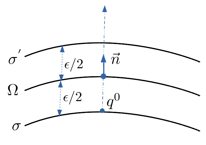
Figure 1: Coordinate System

The co-ordinate system we use here is similar to the one considered by Ogawa Ogawa (2010). We place a curved surface $\Omega$ between the surfaces $\sigma^{{}^{\prime}}$ and $\sigma$ at distances $\epsilon/2$ and $-\epsilon/2$ respectively. Any point between the surfaces $\sigma$ and $\sigma^{{}^{\prime}}$ can be represented by $q^{\mu}=(q^{0},q^{1},q^{2})$ where $(q^{1},q^{2})$ are the curved co-ordinates on the surface $\Omega$ and $q^{0}$ is the normal co-ordinate. The components of the metric $G_{\mu\nu}$ of the curvilinear co-ordinate system can be given as

$$G_{0i}=G_{i0}=0,~{}~{}G_{00}=1,$$

$$G_{ij}=g_{ij}+2q^{0}\kappa_{ij}+(q^{0})^{2}\kappa_{im}\kappa^{m}_{j},$$ (3)

where $g_{ij}$ is the metric on the curved surface $\Omega$, $\kappa_{ij}$ is the second fundamental tensor. The determinant of the metric, $G=\det(G_{\mu\nu}$) can be written as,

$$G_{~{}~{}}=g~{}\{1+2q^{0}\kappa+(q^{0})^{2}(\kappa^{2}+R)+{\cal O}(\epsilon^{3})\},$$ (4)

where, $g=\det(g_{ij})$, mean curvature $\kappa=g^{ij}\kappa_{ij}$ and Ricci scalar $R=(\kappa^{2}-\kappa_{ij}\kappa^{ij})$.

II.1 Effective Theory

In this subsection, we obtain the effective two dimensional description of R-D equations.

The total amount of the chemicals present in the system can be decomposed as follows

$$\int A\sqrt{G}~{}d^{3}q=\int[\int_{-\epsilon/2}^{\epsilon/2}dq^{0}A~{}\sqrt{\frac{G}{g}}~{}]~{}\sqrt{g}~{}d^{2}q,$$ (5)

$$\int B\sqrt{G}~{}d^{3}q=\int[\int_{-\epsilon/2}^{\epsilon/2}dq^{0}B~{}\sqrt{\frac{G}{g}}~{}]~{}\sqrt{g}~{}d^{2}q,$$ (6)

thus leading to a definition of concentrations of chemicals in the effective description

$$\tilde{A}(q^{1},q^{2},t)=\int_{-\epsilon/2}^{\epsilon/2}dq^{0}~{}\sqrt{\frac{G}{g}}~{}A(q^{0},q^{1},q^{2},t),$$ (7)

$$\tilde{B}(q^{1},q^{2},t)=\int_{-\epsilon/2}^{\epsilon/2}dq^{0}~{}\sqrt{\frac{G}{g}}~{}B(q^{0},q^{1},q^{2},t),$$ (8)

Multiplying equations (1) and (2) with $\sqrt{G/g}$ and integrating over $q^{0}$ result in the equations

$$\frac{\partial\tilde{A}}{\partial t}=\tilde{F_{1}}(\tilde{A},\tilde{B})+D_{A}\nabla^{2}_{eff}\tilde{A},$$ (9)

$$\frac{\partial\tilde{B}}{\partial t}=\tilde{F_{2}}(\tilde{A},\tilde{B})+D_{B}\nabla^{2}_{eff}\tilde{B},$$ (10)

where

$$\tilde{F_{1}}(\tilde{A},\tilde{B})=\int_{-\epsilon/2}^{\epsilon/2}dq^{0}~{}\sqrt{\frac{G}{g}}~{}F(A,B),$$ (11)

$$\tilde{F_{2}}(\tilde{A},\tilde{B})=\int_{-\epsilon/2}^{\epsilon/2}dq^{0}~{}\sqrt{\frac{G}{g}}~{}G(A,B),$$ (12)

and

$$\nabla_{eff}^{2}\tilde{A}=\int_{-\epsilon/2}^{\epsilon/2}dq^{0}~{}\sqrt{\frac{G}{g}}~{}\nabla^{2}A,$$ (13)

$$\nabla_{eff}^{2}\tilde{B}=\int_{-\epsilon/2}^{\epsilon/2}dq^{0}~{}\sqrt{\frac{G}{g}}~{}\nabla^{2}B,$$ (14)

If we assume that concentrations of chemicals are independent of $q^{0}$ co-ordinate, then we obtain to ${\cal O}(\epsilon^{2})$

$$\tilde{A}=\epsilon(1+\frac{\epsilon^{2}}{24}R)~{}A(q^{1},q^{2}),$$ (15)

$$\tilde{B}=\epsilon(1+\frac{\epsilon^{2}}{24}R)~{}B(q^{1},q^{2}),$$ (16)

and hence equations (11) and (12) can be rewritten as

$$\tilde{F_{1}}(\tilde{A},\tilde{B})\!\!\! = \!\!\!\epsilon(1\!\!+\!\!\frac{\epsilon^{2}}{24}R)F_{1}(\frac{1}{\epsilon}(1\!-\!\frac{\epsilon^{2}}{24}R)\tilde{A},\frac{1}{\epsilon}(\!1-\!\frac{\epsilon^{2}}{24}R)\tilde{B}),$$

$$\tilde{F_{2}}(\tilde{A},\tilde{B})\!\!\! = \!\!\!\epsilon(1\!+\!\frac{\epsilon^{2}}{24}R)F_{2}(\frac{1}{\epsilon}(1\!-\!\frac{\epsilon^{2}}{24}R)\tilde{A},\frac{1}{\epsilon}(1\!-\!\frac{\epsilon^{2}}{24}R)\tilde{B}).$$

Assuming the fluxes $\nabla A$ and $\nabla B$ vanish at boundaries $\sigma$ and $\sigma^{{}^{\prime}}$, and following similar steps as in Ogawa (2010) for the equations (13) and (14) will lead to

$$\nabla_{eff}^{2} = \Delta^{(2)}+\tilde{\nabla}$$ (19)

$$\tilde{\nabla} = \frac{\epsilon^{2}}{12}g^{-1/2}\frac{\partial}{\partial q^{i}}~{}g^{1/2}$$

$$\times \{(3\kappa^{im}\kappa_{m}^{j}-2\kappa\kappa^{ij})\frac{\partial}{\partial q^{j}}-\frac{1}{2}g^{ij}\frac{\partial R}{\partial q^{j}}\}.$$

where $\Delta^{(2)}$ is the Laplace-Beltrami operator on the curved surface $\Omega$. To summarize, the effective description is captured in (9),(10),(17),(18) and (19).

III Effect of thickness and curvature

In this section, we illustrate the effect of the thickness and curvature in the effective description of a R-D equation. In particular, how does the nature of steady state vary by changing the thickness?. This question can be addressed within the framework of above discussed effective theory. Note that, the thickness is kept constant during the dynamics of the system.

In flat geometries, it can be seen from equations (15) and (16), both the concentration are scaled, $A\rightarrow\epsilon A$ and $B\rightarrow\epsilon B$, and dynamics remains the same. While in curved geometries, combined role of thickness and curvature can lead to nontrivial effects.

In the following, we consider a R-D system between two curved surfaces, and point out some salient features of the effective description. We then proceed to analyze the effective description on spherical, and cylindrical geometry.

III.1 General surface

Let us restrict to the well-studied Schnakenberg model, where the reaction kinetics is taken as Schnakenberg (1979)

$$F_{1}(A,B)=k_{1}-k_{2}A+k_{3}A^{2}B,$$ (20)

$$F_{2}(A,B)=k_{4}-k_{3}A^{2}B,$$ (21)

Here, we confine the chemicals between two curved surfaces $\sigma$ and $\sigma^{{}^{\prime}}$ placed at a distance $\frac{\epsilon}{2}$ from a general curved surface $\Omega$. We can read the effective description of Schnakenberg model on a general surface using equations (17) and (18), and is given by

$$\frac{\partial\tilde{A}}{\partial t} = \tilde{k}_{1}-\tilde{k}_{2}\tilde{A}+\tilde{k}_{3}\tilde{A}^{2}\tilde{B}+D_{A}\nabla^{2}_{eff}\tilde{A},$$ (22)

$$\frac{\partial\tilde{B}}{\partial t} = \tilde{k}_{4}-\tilde{k}_{3}\tilde{A}^{2}\tilde{B}+D_{B}\nabla^{2}_{eff}\tilde{B},$$ (23)

where $\nabla^{2}_{eff}$ is given by (19), and the reaction constants in effective theory are related to the original model as

$$\tilde{k}_{1} = \epsilon k_{1}(1+\frac{\epsilon^{2}}{24}R),~{}\tilde{k}_{3}=\frac{1}{\epsilon^{2}}k_{3}(1-\frac{\epsilon^{2}}{12}R),~{}$$

$$\tilde{k}_{4} = \epsilon k_{4}(1+\frac{\epsilon^{2}}{24}R),~{}\tilde{k}_{2}=k_{2}~{}.$$

In general, the reaction constants in an effective theory of the Schnakenberg model are space-dependent as the Ricci scalar$(R)$ is not necessarily a constant, and may lead to interesting consequences. The space-dependent reaction kinetics can result in an absence of a homogeneous steady state.

A few comments about the dependence of reaction rates on Ricci scalar follows. The term $\tilde{k}_{3}\tilde{A}^{2}\tilde{B}$ in equation (22) represents the production of the chemical $\tilde{A}$. Note that the reaction constant $\tilde{k}_{3}$ is lower in regions with higher positive curvature. Hence, the production of $\tilde{A}$ is more in regions with lower positive curvature. Similarly the term -$\tilde{k}_{3}\tilde{A}^{2}\tilde{B}$ in equation (23) represents the depletion of $\tilde{B}$ and hence can result in more depletion in regions of lower positive curvature. Both the reaction constants $\tilde{k}_{1}$ and $\tilde{k}_{4}$ are higher in regions with higher positive curvature and result in more production of chemicals in these regions.

The term $D_{A}\nabla_{eff}^{2}$ can be rewritten as

$$\frac{1}{\sqrt{g}}\partial_{i}\sqrt{g}(D_{\tilde{A}}^{ij}\partial_{j}\tilde{A}-\frac{\epsilon^{2}}{24}g^{ij}\partial_{j}R.\tilde{A}),$$ (24)

where

$$D_{\tilde{A}}^{ij}=D_{A}(g^{ij}+\frac{\epsilon^{2}}{12}\{3\kappa^{im}\kappa_{m}^{j}-2\kappa\kappa^{ij}\}).$$ (25)

The first term in equation (24) is the diffusion term, which is not necessarily isotropic, and is characterized by the diffusion matrix $D^{ij}$ which depends on the extrinsic curvature. On a sphere the ${\cal O}(\epsilon^{2})$ term of both $D^{\theta\theta}$ and $D^{\phi\phi}$ is negative, where $(\theta,\phi)$ are the co-ordinates on the surface of a sphere. But on a cylindrical surface the ${\cal O}(\epsilon^{2})$ term of $D^{\theta\theta}$ is positive and $D^{zz}=0$, where $(\theta,z)$ are the co-ordinates on the surface of a cylinder. Hence there is an enhanced diffusion of chemicals along the the $\theta$ direction on a locally cylindrical region. The diffusion of chemical can be slow down along $\theta$ and $\phi$ directions on locally spherical regions. The second term in the equation (24) is the current due to the gradient of Ricci scalar between two points on a surface Ogawa (2010).

III.2 Spherical Geometry

We now consider the Schnakenberg model, where the chemicals are confined to the region between two spheres of radii $a_{0}+\frac{\epsilon}{2}$ and $a_{0}-\frac{\epsilon}{2}$. Choose the sphere with radius $a_{0}$ as the surface $\Omega$ and spheres with radii $a_{0}+\frac{\epsilon}{2}$ and   $a_{0}-\frac{\epsilon}{2}$ are the surfaces $\sigma^{{}^{\prime}}$ and $\sigma$, respectively. Our analysis suggests the following effective description for this model

$$\frac{\partial\tilde{A}}{\partial t}=\tilde{k_{1}}-\tilde{k_{2}}\tilde{A}+\tilde{k_{3}}\tilde{A}^{2}\tilde{B}+\nabla^{2}_{eff}\tilde{A},$$ (26)

$$\frac{\partial\tilde{B}}{\partial t}=\tilde{k_{4}}-\tilde{k_{3}}\tilde{A}^{2}\tilde{B}+\nabla^{2}_{eff}\tilde{B},$$ (27)

where the reaction constants in the effective theory are related to original model as follows

$$\tilde{k_{1}} = k_{1}\epsilon(1+\frac{\epsilon^{2}}{24a_{0}^{2}}),~{}\tilde{k_{3}}=\frac{1}{\epsilon^{2}}k_{3}(1-\frac{\epsilon^{2}}{12a_{0}^{2}}),~{}$$

$$\tilde{k_{4}} = k_{4}\epsilon(1+\frac{\epsilon^{2}}{24a_{0}^{2}}),~{}\tilde{k_{2}}=k_{2}~{},$$

since $R=1/a_{0}^{2}$ for the sphere of radius $a_{0}$.
Choosing the $(\theta,\phi)$ coordinates on the surface of a sphere with radius $a_{0}$, it is straightforward to obtain

$$g_{\theta\theta}=a_{0}^{2},g_{\phi\phi}=a_{0}^{2}\sin^{2}\theta,g_{\theta\phi}=g_{\phi\theta}=0,$$

$$\kappa_{\theta\theta}=-a_{0},\kappa_{\phi\phi}=-a_{0}\sin^{2}\theta,\kappa_{\theta\phi}=\kappa_{\phi\theta}=0,$$

$$\kappa_{\phi}^{\phi}=\frac{-1}{a_{0}},\kappa_{\theta}^{\theta}=\frac{-1}{a_{0}},\kappa_{\theta}^{\phi}=\kappa_{\phi}^{\theta}=0.$$

Hence $\nabla^{2}_{eff}$ read as

$$\nabla^{2}_{eff}=\frac{1}{b_{0}^{2}}\{\frac{\partial^{2}}{\partial\phi^{2}}+\frac{1}{\sin\theta}\frac{\partial}{\partial\theta}(\sin\theta~{}\frac{\partial}{\partial\theta})\},$$ (28)

where $b_{0}=a_{0}(1+\frac{\epsilon^{2}}{24a_{0}^{2}})$. In essence, the effective two dimensional R-D equations (26) and (27) can be interpreted as Schnakenberg model on a sphere of radius $b_{0}$ with redefined parameters.

Equations (26) and (27) can be rewritten in terms of rescaled variables as

$$\frac{\partial U}{\partial\tau}=\gamma(a-U+U^{2}~{}V)+\tilde{\nabla}_{eff}^{2}U,$$ (29)

$$\frac{\partial V}{\partial\tau}=\gamma(b-U^{2}~{}V)+d~{}\tilde{\nabla}_{eff}^{2}{V},$$ (30)

where,

$$\tau=D_{A}t/b_{0}^{2},U=\tilde{A}(\frac{\tilde{k}_{3}}{\tilde{k}_{2}})^{1/2},~{}V=\tilde{B}(\frac{\tilde{k}_{3}}{\tilde{k}_{2}})^{1/2},~{}d=\frac{D_{B}}{D_{A}},$$

(31)

$$a=(\frac{\tilde{\kappa}_{1}}{\tilde{k}_{2}})(\frac{\tilde{k}_{3}}{\tilde{k}_{2}})^{1/2},~{}b=(\frac{\tilde{k}_{4}}{\tilde{k}_{2}})(\frac{\tilde{\kappa}_{3}}{\tilde{k}_{2}})^{1/2},~{}\gamma=\frac{b_{0}^{2}\tilde{\kappa_{2}}}{D_{A}}.$$

and $\tilde{\nabla}_{eff}^{2}$ is the Laplace operator in the scaled variables.

The homogeneous steady state solution can be obtained from (29) and (30) as $(U_{0},V_{0})=(a+b,\frac{b}{(a+b)^{2}})$. We consider only positive solution of homogeneous steady state and discard the solution with negative concentration. Note that homogeneous steady state solution is independent of the thickness to ${\cal O}(\epsilon^{2})$.

The linear stability analysis about the homogeneous steady state follows. A small variation in the homogeneous steady state is denoted as

$$\delta W=\left(\begin{array}[]{c}\delta U-U_{0}\\ \delta V-V_{0}\\ \end{array}\right),$$

which satisfies the linearized equation

$$\frac{\partial~{}(\delta W)}{\partial t}=\hat{L}\delta W,$$ (32)

where

$$\hat{L}=\gamma C+D\nabla_{eff}^{2},$$ (33)

$$D=\left(\begin{array}[]{cc}1&0\\ 0&d\\ \end{array}\right),C=\left(\begin{array}[]{cc}\frac{\partial f}{\partial U}&\frac{\partial f}{\partial V}\\ \\ \frac{\partial g}{\partial U}&\frac{\partial g}{\partial V}\\ \end{array}\right)_{U_{0},V_{0}},$$

and

$$f(U,V)=\gamma(a-U+U^{2}~{}V),$$

$$g(U,V)=\gamma(b-U^{2}~{}V)~{}.$$

The solution to the equation (32) can be written as

$$\delta W(\theta,\phi,t)=\sum_{l=0}^{l=\infty}\sum_{m=-l}^{l}C_{l}^{m}e^{\lambda(l)t}P_{l}^{m}(\cos\theta)e^{im\phi},$$ (34)

where the constants $C_{l}^{m}$ can be determined from initial conditions. The eigenvalues $\lambda(l)$ satisfy

$$\lambda^{2}+\lambda[(l(l+1))(1+d)-\gamma(f_{u}+g_{v})]+h(l(l+1))=0,$$ (35)

where $f_{u}=\frac{\partial f}{\partial U}$, $g_{v}=\frac{\partial g}{\partial V}$ and $h(l(l+1))$ can be given as

$$h(l(l+1))=d(l(l+1))^{2}-\gamma(d~{}f_{u}+g_{v})~{}l(l+1)+\gamma^{2}(f_{u}g_{v}-f_{v}g_{u}).$$ (36)

The necessary condition for the instability to kick in is

$$h(l(l+1))<0,$$

The modes $l$ which satisfy $h(l(l+1))<0$ gives positive eigenvalues in equation (35). These are the modes which give rise to the instability (an inhomogeneous steady state) to the system. These modes(unstable modes) lie between $L_{-}<l(l+1)<L_{+}$, where $L_{-}$ and $L_{+}$ are the roots of $h(l(l+1))=0$, and given as

$$L_{\pm}(\epsilon)=\frac{a_{0}^{2}\tilde{k_{2}}}{D_{A}.2d}(1+\frac{\epsilon^{2}}{12a_{0}^{2}})[(df_{u}+g_{v})$$

$$\pm\{(df_{u}+g_{v})^{2}-4d(f_{u}g_{v}-f_{v}g_{u})\}^{1/2}].$$ (37)

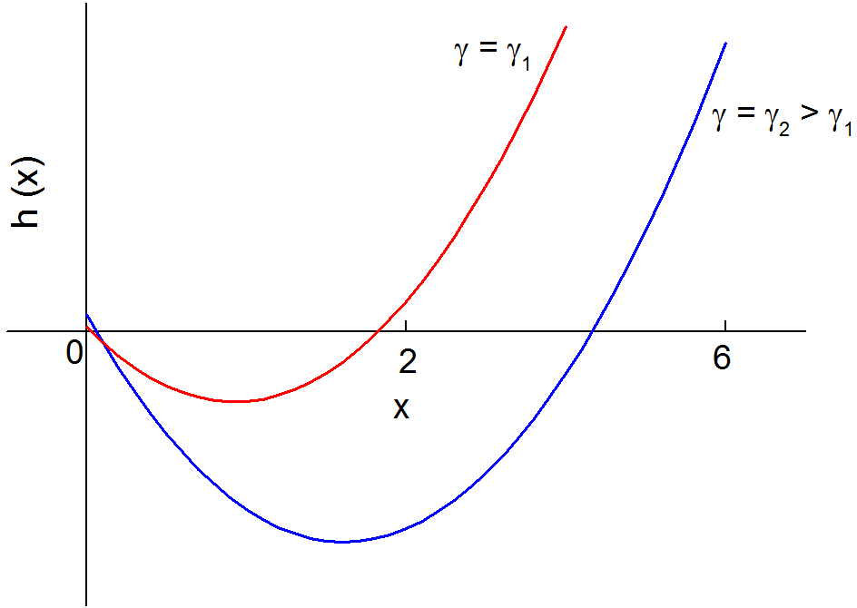
Figure 2: h(x) Vs x: Figure illustrates the role of thickness-dependent $\gamma$ in the selection of unstable modes.

Note that the unstable modes lie between the zeros$(L_{+},L_{-})$ of the function $h(x)$, where $L_{+}$ and $L_{-}$ depend on the thickness. It can be seen from the equation (37) that an increase(decrease) in thickness can shift the zeros of $h(x)$ towards right(left) on the $x$ axis as shown in the fig(2), and this can result in a scenario where the stable modes can become unstable and vice versa. Hence the nature of steady state can be changed by tuning the thickness. In other words, there can be a transition from a homogeneous steady state to an inhomogeneous steady state(a pattern) by changing the thickness. It is also possible to obtain different inhomogeneous steady states as thickness changes. The $\epsilon$ dependence in the equation (37) thus reveals the effect of thickness on the stability.

Let us distinguish two cases. In the case I, for certain ranges of parameters(a,b,d,$\gamma$) the zeros of function $h(x)$ lie below the point $x=2$, namely, $0<L_{-}$ and $L_{+}<2$. Here, the steady state configuration is homogeneous. In this case, since there is no unstable mode lies below the point $x=2$, the instability can set in only by increasing the thickness.

In the case II, the zeros of function $h(x)$ lie between $l_{1}(l_{1}+1)$ and $(l_{1}+1)(l_{1}+2)$, namely, $l_{1}(l_{1}+1)<L_{-}$ and $L_{+}<(l_{1}+1)(l_{1}+2)$. In this case the system can be driven to an inhomogeneous steady state either by decreasing or increasing the thickness.

III.3 Cylindrical Geometry

Here we consider Schnakenberg model, where the chemicals are confined between two cylinders of radii $a_{0}+\frac{\epsilon}{2}$ and $a_{0}-\frac{\epsilon}{2}$, and further assume the flux vanishes at $z=0$ and $z=l$.

In this case the effective description is governed by

$$\frac{\partial\tilde{A}}{\partial t} = \tilde{\kappa}_{1}-\tilde{\kappa}_{2}\tilde{A}+\tilde{\kappa}_{3}\tilde{A}^{2}\tilde{B}+\nabla^{2}_{eff}\tilde{A},$$ (38)

$$\frac{\partial\tilde{B}}{\partial t} = \tilde{\kappa}_{4}-\tilde{\kappa}_{3}\tilde{A}^{2}\tilde{B}+\nabla^{2}_{eff}\tilde{B},$$ (39)

where the reaction constants in the effective theory are related to the original model as follows

$$\tilde{k}_{1}=k_{1}\epsilon,~{}\tilde{k}_{3}=\frac{1}{\epsilon^{2}}k_{3},~{}\tilde{k}_{4}=k_{4}\epsilon,~{}\tilde{k}_{2}=k_{2}~{}.$$

on the surface of a cylinder with radius $a_{0}$ the quantities related to intrinsic and extrinsic curvatures are

$$g_{\theta\theta}=a_{0}^{2},g_{zz}=1,g_{\theta z}=g_{z\theta}=0,$$

$$\kappa_{\theta\theta}=a_{0},\kappa_{zz}=0,\kappa_{\theta z}=\kappa_{z\theta}=0,$$

$$\kappa^{\theta\theta}=\frac{1}{a_{0}^{3}},\kappa^{zz}=0,\kappa^{\theta z}=0.$$

Hence,

$$\nabla^{2}_{eff}=\frac{1}{b_{0}^{2}}\frac{\partial^{2}}{\partial\theta^{2}}+\frac{\partial^{2}}{\partial z^{2}},$$ (40)

where $b_{0}=a_{0}\{1-\frac{\epsilon^{2}}{24a_{0}^{2}}\}$. Thus the effective equations  (38) and (39) can be interpreted as Schnakenberg model on a cylinder with rescaled radius $b_{0}$. Equations (38) and (39) can be rewritten in terms of rescaled variables, $U=U(\theta,\tilde{z})$, and $V=V(\theta,\tilde{z})$, obeying the equations

$$\frac{\partial U}{\partial\tau}=\gamma(a-U+U^{2}~{}V)+\tilde{\nabla}_{eff}^{2}U,$$ (41)

$$\frac{\partial V}{\partial\tau}=\gamma(b-U^{2}~{}V)+d~{}\tilde{\nabla}_{eff}^{2}{V}~{},$$ (42)

where the scaled variables are defined in equation (31) and $\tilde{z}=\frac{z}{b_{0}}$, and $\tilde{\nabla}_{eff}^{2}$ is Laplace operator in the scaled variables.

If we now proceed similar to the case of a sphere, then the deviation from homogeneous solution

$$\delta W(\theta,\tilde{z},t)=\sum_{n,m}C_{nm}e^{\lambda t}e^{in\theta}\cos(\frac{m\pi b_{0}}{l}\tilde{z}),$$ (43)

where $C_{nm}$ depends on the initial conditions. The eigenvalues can be obtained from

$$\lambda^{2}+\lambda[(n^{2}+\frac{m^{2}\pi^{2}b_{0}^{2}}{l^{2}})(1+d)-\gamma(f_{u}+g_{v})]+h(n,m)=0,$$

where

$$h(n,m)=d\{n^{2}+\frac{m^{2}\pi^{2}b_{0}^{2}}{l^{2}}\}^{2}-\gamma(d~{}f_{u}+g_{v})(n^{2}+\frac{m^{2}\pi^{2}b_{0}^{2}}{l^{2}})$$

$$~{}+\gamma^{2}(f_{u}g_{v}-f_{v}g_{u}).$$

Following the same analysis as done in the case of a sphere, the modes (n,m) which satisfy the following condition

$$R_{-}^{2}<(n^{2}+\frac{m^{2}\pi^{2}b_{0}^{2}}{l^{2}})<R_{+}^{2},$$ (44)

will destabilize the homogeneous solution, where $R_{-}^{2}$ and $R_{+}^{2}$ are the zeros of $h(n,m)$ and given by

$$R_{\pm}^{2}(\epsilon)=\frac{a_{0}^{2}\tilde{k_{2}}}{D_{A}.2d}(1-\frac{\epsilon^{2}}{12a_{0}^{2}})[(df_{u}+g_{v})$$

$$\pm\{(df_{u}+g_{v})^{2}-4d(f_{u}g_{v}-f_{v}g_{u})\}^{1/2}]~{}.$$ (45)

Hence the unstable modes $\displaystyle(n,m)$ lie between the two semicircles in the $\displaystyle(n,\frac{m\pi b_{0}}{l})$ plane with radius $R_{+}$ and $R_{-}$ as shown in the figure 3. It can be seen from equation (45) that the values of both $R_{-}$ and $R_{+}$ decrease by increasing the thickness($\epsilon$).

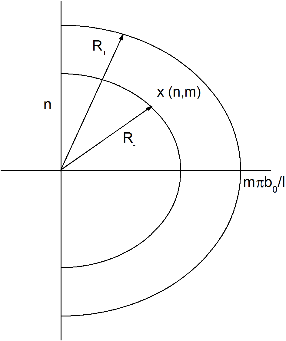
Figure 3: Unstable modes $(n,m)$ lie between semicircles with radius $R_{-}$ and $R_{+}$.

Let us distinguish two cases. In the case I, the space between two semicircles in the $(n,\frac{m\pi b_{0}}{l})$ plane encloses no mode $(n,m)$ satisfying the condition (44). The steady state configuration of R-D system is homogeneous in this case. By increasing the thickness the semicircles can shrink, and can result in the inclusion of some modes $(n,m)$. Hence, there is a possibility of obtaining an inhomogeneous steady state from the homogeneous one by increasing the thickness. It is also possible in this case that the region between two circles can encompass no modes $(n,m)$ even after increasing the thickness. In such a situation, the system can continue to be in the homogeneous steady state.

In the case II, some modes $(n,m)$ are enclosed within the semicircles of radius $R_{+}$ and $R_{-}$. The steady state configuration is inhomogeneous in this case. Now an increase in thickness can result in the shifting of curves such that modes $(n,m)$ are no longer present between $R_{-}$ and $R_{+}$ semicircles. Hence, there is a possibility of transition to a homogeneous steady state from an inhomogeneous one by increasing the thickness. Another possibility is that the semicircles can shrink. This can lead to an inclusion of new modes $(n,m)$ and result in transition to a new inhomogeneous steady state from the initial inhomogeneous state.

IV Conclusion

To conclude, we have studied the effect of curvature and thickness in R-D systems on quasi-two dimensional(thick) curved surfaces. We explicitly analyzed an effective description of the Schnakenberg model, in particular, on spherical and cylindrical geometry. In both spherical and cylindrical case, the effective theory is same as the original model on a sphere and a cylinder, respectively, with rescaled parameters. On the spherical geometry an increase in the thickness can lead to an increase in the parameter $\gamma$. In cylindrical geometry the parameter $\gamma$ can decrease by increasing the thickness. In the absence of curvature, the thickness play no significant role in the effective description.

In general, R-D systems on quasi-two dimensional curved surfaces can have space-dependent parameters. There are a few instances where spatially varying parameters are considered Page et al. (2005); Bhattacharyay and Bhattacharjee (1999); Page et al. (2003); Benson et al. (1993); Mau et al. (2012). The absence of homogeneous steady state is also a characteristic of the effective R-D equation. The effective R-D description is not necessarily similar to the original description on a two-dimensional surface with rescaled parameters. In R-D systems on quasi-two dimensional curved surfaces, a change in thickness can stabilize the unstable patterns and vice versa. Hence the patterns (inhomogeneous steady state) can appear or disappear by tuning the thickness. This might be a plausible reason for different patterns on leopards and jaguars Liu et al. (2006) as they grow in size or rather as the skin thickness increases.

There is a related model studied in the context of Belousov-Zhabotinsky reaction Rovinsky and Menzinger (1992) where there is no diffusion. Instead, equation to the chemical $A$ contain $v.\nabla A$ term, where $v$ is the velocity of the chemical $A$, while the other chemical $B$ is immobilized. In this model the chemical instability is of traveling-wave type, and the concentrations can vary both in space and time. In this case there is an isotropy in the wave speed when the speed of the chemical $A$ is same in every directions. Assume that the velocity$(v)$ of the chemical $A$ is independent of the $q^{0}$ direction. Then following the methods described in sec.II, one can straightforwardly obtain the effective description of the above model on an infinite cylinder. The stability analysis follows provided the linear terms in the reaction kinetics of the effective theory meet the stability condition. The above analysis shows that the thickness can induce an anisotropy in the speed of the traveling-wave.

The effective description outline in the paper can be easily extended to any R-D models like Gierer-Meinhardt model Gierer and Meinhardt (1972), and other R-D models Murray (2001); Koch and Meinhardt (1994); Maini et al. (1997). The analysis may prove useful in the study of the rearrangement of spatial patterns during various stages of growth in animals. Turing-like models also find applications in diverse areas like material sciences Krinsky (1984), hydrodynamics White (1988), astrophysics Nozakura and Ikeuchi (1984), etc. In these systems, under certain conditions it is conceivable that the thickness and curvature can play a significant role, and hence similar effective descriptions may be suitable.

V ACKNOWLEDGEMENT

I acknowledge Sreedhar Dutta for suggesting the problem, and for extensive discussions. I also thank him for various helpful suggestions during the preparation of the manuscript.

References

Turing (1952)
A. M. Turing,
Philosophical Transactions of the Royal Society of London
B: Biological Sciences 237, 37
(1952).
Murray (2001)
J. D. Murray,
Mathematical Biology. II Spatial Models and Biomedical
Applications Interdisciplinary Applied Mathematics V. 18
(Springer-Verlag New York Incorporated,
2001).
Koch and Meinhardt (1994)
A. Koch and
H. Meinhardt,
Reviews of modern physics 66,
1481 (1994).
Shoji et al. (2002)
H. Shoji,
Y. Iwasa,
A. Mochizuki,
and S. Kondo,
Journal of Theoretical Biology
214, 549 (2002).
Bard (1981)
J. B. Bard,
Journal of Theoretical Biology
93, 363 (1981).
Murray and Myerscough (1991)
J. D. Murray and
M. Myerscough,
Journal of theoretical biology
149, 339 (1991).
Liu et al. (2006)
R. Liu,
S. Liaw, and
P. Maini,
Physical review E 74,
011914 (2006).
Varea et al. (1999)
C. Varea,
J. Aragon, and
R. Barrio,
Physical Review E 60,
4588 (1999).
Nelson et al. (2006)
C. M. Nelson,
M. M. VanDuijn,
J. L. Inman,
D. A. Fletcher,
and M. J.
Bissell, Science
314, 298 (2006).
Halbedel et al. (2009)
S. Halbedel,
L. Visser,
M. Shaw,
L. J. Wu,
J. Errington,
D. Marenduzzo,
L. W. Hamoen,
et al., The EMBO journal
28, 2272 (2009).
Peter et al. (2004)
B. J. Peter,
H. M. Kent,
I. G. Mills,
Y. Vallis,
P. J. G. Butler,
P. R. Evans, and
H. T. McMahon,
Science 303,
495 (2004).
Gov and Gopinathan (2006)
N. S. Gov and
A. Gopinathan,
Biophysical journal 90,
454 (2006).
Orlandini et al. (2013)
E. Orlandini,
D. Marenduzzo,
and
A. Goryachev,
Soft Matter 9,
9311 (2013).
Ogawa (2010)
N. Ogawa,
Physical review E 81,
061113 (2010).
Balois et al. (2014)
T. Balois,
C. Chatelain,
and M. B. Amar,
Journal of The Royal Society Interface
11, 20140339
(2014).
Schnakenberg (1979)
J. Schnakenberg,
Journal of theoretical biology
81, 389 (1979).
Page et al. (2005)
K. M. Page,
P. K. Maini, and
N. A. Monk,
Physica D: Nonlinear Phenomena
202, 95 (2005).
Bhattacharyay and Bhattacharjee (1999)
A. Bhattacharyay
and
J. Bhattacharjee,
The European Physical Journal B-Condensed Matter and
Complex Systems 8, 137
(1999).
Page et al. (2003)
K. Page,
P. K. Maini, and
N. A. Monk,
Physica D: Nonlinear Phenomena
181, 80 (2003).
Benson et al. (1993)
D. Benson,
P. Maini, and
J. Sherratt,
Mathematical and computer modelling
17, 29 (1993).
Mau et al. (2012)
Y. Mau,
A. Hagberg, and
E. Meron,
Physical review letters 109,
034102 (2012).
Rovinsky and Menzinger (1992)
A. B. Rovinsky and
M. Menzinger,
Physical Review Letters 69,
1193 (1992).
Gierer and Meinhardt (1972)
A. Gierer and
H. Meinhardt,
Kybernetik 12,
30 (1972).
Maini et al. (1997)
P. Maini,
K. Painter, and
H. P. Chau,
Journal of the Chemical Society, Faraday Transactions
93, 3601 (1997).
Krinsky (1984)
V. Krinsky,
Self-organization: autowaves and structures far from
equilibrium (Springer, 1984).
White (1988)
D. B. White,
Journal of Fluid Mechanics 191,
247 (1988).
Nozakura and Ikeuchi (1984)
T. Nozakura and
S. Ikeuchi,
The Astrophysical Journal 279,
40 (1984).