A Scalable and Extensible Framework for Superposition-Structured Models

Abstract

In many learning tasks, structural models usually lead to better interpretability and higher generalization performance. In recent years, however, the simple structural models such as lasso are frequently proved to be insufficient. Accordingly, there has been a lot of work on “superposition-structured” models where multiple structural constraints are imposed. To efficiently solve these “superposition-structured” statistical models, we develop a framework based on a proximal Newton-type method. Employing the smoothed conic dual approach with the LBFGS updating formula, we propose a scalable and extensible proximal quasi-Newton (SEP-QN) framework. Empirical analysis on various datasets shows that our framework is potentially powerful, and achieves super-linear convergence rate for optimizing some popular “superposition-structured” statistical models such as the fused sparse group lasso.

1 Introduction

In this paper, we consider the “superposition-structured” statistical models (?) where multiple structural constraints are imposed. Examples of such structural constraints include sparsity constraint, graph-structure, group-structure, etc. We could leverage such structural constraints via specific regularization functions. Consequently, many problems of relevance in “superposition-structured” statistical learning can be formulated as minimizing a composite function:

$$\min_{\mathbf{x}\in\mathbb{R}^{p}}f(\mathbf{x})\triangleq g(\mathbf{x})+\Psi(\mathbf{x}),$$ (1)

where $g$ is a convex and continuously differentiable loss function, and $\Psi$ is a hybrid regularization, usually defined as sum of $N$ convex (non-smooth) functions. More specifically,

$$\Psi(\mathbf{x})\triangleq\sum_{i=1}^{N}\psi_{i}(\mathbf{W}_{i}\mathbf{x}+\mathbf{b}_{i}),$$

each $\psi_{i}$ is convex but not necessarily differentiable, $\mathbf{W}_{i}\in\mathbb{R}^{q_{i}\times p}$ and $\mathbf{b}_{i}\in\mathbb{R}^{q_{i}}$ are available. For example, $\Psi(\mathbf{x})\triangleq\lambda_{1}\|\mathbf{x}\|_{1}+\lambda_{2}\|\mathbf{F}\mathbf{x}\|_{1}+\lambda_{3}\sum_{j=1}^{N-2}\|\mathbf{G}_{j}\mathbf{x}\|_{2}$ defines a fused sparse group penalty (?) when $\mathbf{F}$ is the difference matrix and $\mathbf{G}_{j}$ indicates the group.

Indeed, there are plenty of machine learning models, which can be cast into the formulation in (1).

• Generalized lasso model: all generalized lasso models such as the fused lasso (?), the sparse group lasso (?), the group lasso for logistic regression (?) can be written as the following form:

  $$\min_{\mathbf{x}\in\mathbb{R}^{p}}f(\mathbf{x})\triangleq g(\mathbf{x})+\lambda_{1}\|\mathbf{F}\mathbf{x}\|_{1}+\sum_{j=2}^{N}\lambda_{j}\|\mathbf{G}_{j}\mathbf{x}\|_{2}.$$

• Multi-task learning: given $r$ tasks, each with sample matrix $\mathbf{A}^{(k)}\in\mathbb{R}^{(n_{k}\times p)}$ ( samples in the k-th task) and labels $\mathbf{y}^{(k)}$, ? proposed minimizing the following objective:

  $$\min_{\mathbf{x}\in\mathbb{R}^{p}}f(\mathbf{x})\triangleq\sum_{k=1}^{r} l(\mathbf{y}^{(k)},\mathbf{A}^{(k)}(\mathbf{S}^{(k)}+\mathbf{B}^{(k)}))$$

  $$+\lambda_{1}\|\mathbf{S}\|_{1}+\lambda_{2}\|\mathbf{B}\|_{1,\infty},$$ (2)

  where $l(\cdot)$ is the loss function and $\mathbf{S}^{(k)}$ is the k-th column of S. Besides, more multi-task learning like the model in (?) also could be cast into (1).

• Gaussian graphical model with latent variables: ? showed that the precision matrix will have a low rank + sparse structure when some random variables are hidden, thus the “superposition-structured” model will be much helpful.

Moreover, many real-world problems benefit from these models such as Gene expression, time-varying network and disease progression. In this paper we mainly study the computational issue of the model in (1).

There are some generic methods that can be used to solve these models theoretically. The CVX (?) is able to solve these models, but it is not scalable. The Primal-Dual approach proposed by ? (2012) can deal with these models, but it converges slowly. The smoothed conic dual (SCD) approach was studied in (?; ?) and ? (2012) could obtain $\mathcal{O}(\frac{1}{\epsilon})$ iteration-complexity, but it needs to find the minimizer related to $g(\mathbf{x})$ in each iteration. In addition, the alternating direction method of multipliers (ADMM) (?) can also be used to solve this kind of problems. However, ADMM still suffers from the same bottleneck as the methods mentioned earlier. Additionally, as we know that disk I/O is the bottleneck of computation, so it is important to reduce the number of evaluating $g(\mathbf{x})$. In summary, it is challenging to efficiently solve the model on large-scale datasets.

Recently, there has been a flurry of activity about developments of Newton-type methods for minimizing composite functions (1) in the literature. In particular, in (?; ?) the authors focused on minimizing a composite function, which contains a convex smooth function and a convex non-smooth function with a simple proximal mapping. They also analyzed the convergence rate of various proximal Newton-type methods. ? (2011) discussed a projected quasi-Newton algorithm, but the sub-iteration procedure costs too much. ? (2014) further generalized the Newton method to handle some dirty statistical estimators. Their developments “open up the state of the art but forbidding class of M-estimators to very large-scale problems.” In addition, there have already been plenty of packages that implement these Newton-type methods such as LIBLINEAR (?), GLMNET (?; ?), but are limited to solve simple models such as lasso and elastic net.

To solve the “superposition-structured” models in (1) on the large-scale problem, we resort to a proximal quasi-Newton method which converges superlinearly (?). We develop a Scalable and Extensible Proximal Quasi-Newton (SEP-QN) framework to solve these models. More specifically, we apply a smoothed conic dual (SCD) approach to solving a surrogate of the original model (1). We employ the LBFGS updating formula, so that the surrogate problem could be solved not only efficiently but also robust. Moreover, we present several accelerating techniques including adaptive initial Hessian, warm-start and continuation SCD to solve the surrogate problem more efficiently and gain faster convergence rate.

In the following we start by presenting our SEP-QN framework for solving the “superposition-structured” statistical models. Then we present the approach to solve the surrogate problem, followed by theoretical analysis and concluding empirical analysis.

2 The SEP-QN Framework

In this section we present the SEP-QN framework for solving the “superposition-structured” statistical model in (1). We refer to $g(\mathbf{x})$ as “smooth part” and $\Psi(\mathbf{x})$ as “non-smooth part.” Usually, $g(\mathbf{x})$ is a loss function. For example, $g(\mathbf{x})\triangleq\frac{1}{n}\sum_{i=1}^{n}(y_{i}{-}{\bf a}_{i}^{T}\mathbf{x})^{2}$ in the least squares regression problem where the ${\bf a}_{i}\in\mathbb{R}^{p}$ are input vectors and $y_{i}\in\mathbb{R}$ are the corresponding outputs, and $g(\mathbf{x})\triangleq\frac{1}{n}\sum_{i=1}^{n}\log(1+\exp(-y_{i}{\bf a}_{i}^{T}\mathbf{x}))$ in the logistic regression where the $y_{i}\in\{-1,1\}$. We are especially interested in the large-scale case; i.e., the number of training data $n$ is large.

Basic Framework

Roughly speaking, the method is built on a line search strategy, which produces a sequence of points $\{\mathbf{x}_{k}\}$ according to

$$\mathbf{x}_{k+1}=\mathbf{x}_{k}+t_{k}\Delta\mathbf{x}_{k},$$

where $t_{k}$ is a step length calculated by backtrack, and $\Delta\mathbf{x}_{k}$ is a descent direction. We compute the descent direction by minimizing a surrogate $\hat{f}_{k}$ of the objective function $f$. Given the $k$th estimate $\mathbf{x}_{k}$ of $\mathbf{x}$, we let $\hat{f}_{k}(\mathbf{x})$ be a local approximation of $f$ around $\mathbf{x}_{k}$. The descent direction $\Delta\mathbf{x}_{k}$ is obtained by solving the following surrogate problem:

$$\min_{\mathbf{x}}\;\hat{f}_{k}(\mathbf{x}).$$ (3)

Proximal Newton-type methods approximate only the smooth part $g$ with a local quadratic form. Thus, in this paper the surrogate function is defined by

$$\hat{f_{k}}(\mathbf{x})=~{} \hat{g}_{k}(\mathbf{x})+\Psi(\mathbf{x})$$

$$=~{} g(\mathbf{x}_{k})+\nabla g(\mathbf{x}_{k})^{T}(\mathbf{x}-\mathbf{x}_{k})$$

$$+\frac{1}{2}(\mathbf{x}-\mathbf{x}_{k})^{T}\mathbf{H}_{k}(\mathbf{x}-\mathbf{x}_{k})+\Psi(\mathbf{x}),$$ (4)

where $\mathbf{H}_{k}$ is a $p\times p$ positive definite matrix as approximation to the Hessian of $g$ at $\mathbf{x}=\mathbf{x}_{k}$. There are many strategies for choosing $\mathbf{H}_{k}$, such as BFGS and LBFGS (?). Considering the use in the large-scale problem, we will employ LBFGS to compute $\mathbf{H}_{k}$.

After we have obtained the minimizer $\hat{\mathbf{x}}_{k}$ of (3), we use the line search procedure such as backtracking to select the step length $t_{k}$ such that a sufficient descent condition is satisfied (?). That is,

$$f(\mathbf{x}_{k}+t_{k}\Delta\mathbf{x}_{k})\leq f(\mathbf{x}_{k})+\alpha t_{k}\gamma_{k},$$ (5)

where $\alpha\in(0,1/2)$, $\Delta\mathbf{x}_{k}\triangleq\hat{\mathbf{x}}_{k}-\mathbf{x}_{k}$, and

$$\gamma_{k}\triangleq\nabla g(\mathbf{x}_{k})^{T}\Delta\mathbf{x}_{k}+\Psi(\mathbf{x}_{k}+\Delta\mathbf{x}_{k})-\Psi(\mathbf{x}_{k}).$$

Algorithm 1 gives the basic framework of SEP-QN. The key is to solve the surrogate problem (3) when there are multiple structural constraints. In Algorithm 2 we present the method of solving the problem (3). Moreover, we develop several techniques to further accelerate our method. Specifically, we propose an acceleration schema by adaptively adjusting the initial Hessian $\mathbf{H}_{0}$ in Algorithm 3. We will see that with an appropriate $\mathbf{H}_{0}$, $\mathbf{H}_{k}$ can be a better approximation of $\nabla^{2}g(\mathbf{x}_{k})$, leading to a much faster convergent procedure.

Algorithm 1 The SEP-QN Framework

1:$\mathbf{x}_{0}$ and $\mathbf{H}_{0}$

2:$\mathbf{x}_{0}\in\mathrm{dom}f$, and $\mathbf{H}_{0}$ is a scaled identity matrix (positive definite).

3:$S\leftarrow[]$, $Y\leftarrow[]$, and $\beta\leftarrow 2$

4:repeat

5:     Update $\mathbf{H}_{k}$ using LBFGS, where $\mathbf{H}_{k}$ is symmetric positive definite.

6:     Solve the problem in (3) for a descent direction:

$$\Delta\mathbf{x}_{k}\leftarrow\operatorname*{argmin}_{\Delta}\hat{f}_{k}(\mathbf{x}_{k}+\Delta)\text{\quad(Alogrithm~{}\ref{alg:sub_scd_solver})}$$

7:     Search $t_{k}$ with backtracking method.

8:     Update $\mathbf{x}_{k+1}\leftarrow\mathbf{x}_{k}+t_{k}\Delta\mathbf{x}_{k}$

9:     if $(\mathbf{x}_{k+1}-\mathbf{x}_{k})^{T}(\nabla g(\mathbf{x}_{k+1})-\nabla g(\mathbf{x}_{k}))>0$ then

10:         $S\leftarrow[S,\mathbf{x}_{k+1}-\mathbf{x}_{k}]$

11:         $Y\leftarrow[Y,\nabla g(\mathbf{x}_{k+1})-\nabla g(\mathbf{x}_{k})]$

12:         $\mathbf{H}_{0}\leftarrow$ $Ada\_Hess(t_{k},\beta,\mathbf{x}_{k+1}-\mathbf{x}_{k},\nabla g(\mathbf{x}_{k+1})-\nabla g(\mathbf{x}_{k}),\mathbf{H}_{0})$ (Algorithm 3)

13:     end if

14:until stopping condition is satisfied

The Solution of the Surrogate Problem (3)

If there is only one non-smooth function in $\Psi(\mathbf{x})$ (i.e., $N$=1) with simple proximal mapping, we can solve the surrogate problem (3) directly and efficiently via various optimal first-order algorithms such as FISTA (?) and coordinate descent which is used in LIBLINEAR (?) and GLMNET (?; ?). In this paper we mainly consider the case that there are multiple non-smooth functions. In this case, we could use SCD or ADMM to solve the problem. Since we empirically observe that SCD outperforms ADMM, we resort to the SCD approach.

The SCD Approach

In order to solve the problem (3) efficiently when $N>1$, we employ the SCD approach. The main idea is to solve the surrogate problem via its dual.

We first reformulate our concerned problem in (3) into the following form:

$${\min}\quad\mathcal{P}(\boldsymbol{\nu})=\hat{g}_{k}(\mathbf{x})+\sum_{i=1}^{N}t_{i}$$ (6)

$$\text{s.t. \quad}(\mathbf{W}_{i}\mathbf{x}+\mathbf{b}_{i},t_{i})\in\mathcal{K}_{\psi_{i}},$$

where $\boldsymbol{\nu}=(\mathbf{x},t_{1},...,t_{N}),t_{i}$ are new scalar variables, and $\mathcal{K}_{\psi_{i}}$ is a closed convex cone (usually the epigraph $\psi_{i}(\mathbf{W}_{i}\mathbf{x}+\mathbf{b}_{i})\leq t_{i}$). Since projection onto the set $\{\mathbf{x}|(\mathbf{W}_{i}\mathbf{x}+\mathbf{b}_{i},t_{i})\in\mathcal{K}_{\psi_{i}}\}$ might be expensive, we address this issue by solving the dual problem.

We denote the dual variables by $\boldsymbol{\lambda}=(\mathbf{z}_{1},\tau_{1},...,\mathbf{z}_{N},\tau_{N})$, $\mathbf{z}=(\mathbf{z}_{1},...,\mathbf{z}_{N})$, where $(\mathbf{z}_{i},\tau_{i})\in\mathcal{K}_{\psi_{i}}^{*}$. And $\mathcal{K}_{\psi_{i}}^{*}$ is the dual cone defined by

$$\mathcal{K}_{\psi_{i}}^{*}=\{\mathbf{x}:\mathbf{x}^{T}\mathbf{y}\geq 0\text{~{}for all }\mathbf{y}\in\mathcal{K}_{\psi_{i}}\}.$$

Let us take an example in which $\psi_{i}(\mathbf{x})=\|\mathbf{W}_{i}\mathbf{x}+\mathbf{b}_{i}\|_{1}\leq t_{i}$. Then $\mathcal{K}_{\psi_{i}}=\{(\mathbf{W}_{i}\mathbf{x}+\mathbf{b}_{i},t_{i}):\|\mathbf{W}_{i}\mathbf{x}+\mathbf{b}_{i}\|_{1}\leq t_{i}\}$ and $\mathcal{K}_{\psi_{i}}^{*}=\{(\mathbf{z}_{i},\tau_{i}):\|\mathbf{z}_{i}\|_{\infty}\leq\tau_{i}\}$.

The Lagrangian and dual functions are given by

$$\mathcal{L}(\boldsymbol{\nu};\boldsymbol{\lambda}) =\hat{g}_{k}(\mathbf{x})+\sum_{i=1}^{N}(t_{i}-\mathbf{z}_{i}^{T}(\mathbf{W}_{i}\mathbf{x}+\mathbf{b}_{i})-\tau_{i}t_{i}),$$

$$\mathcal{D}(\boldsymbol{\lambda}) =\inf_{\mathbf{x},t_{i}}\;\Big{\{}\mathcal{L}(\mathbf{x},t_{i};\mathbf{z}_{i},\tau_{i})$$

$$\triangleq\hat{g}_{k}(\mathbf{x})+\sum_{i=1}^{N}(t_{i}-\mathbf{z}_{i}^{T}(\mathbf{W}_{i}\mathbf{x}+\mathbf{b}_{i})-\tau_{i}t_{i})\Big{\}}.$$ (7)

The Lagrangian is unbounded unless $\tau_{i}=1$. Because the appropriate Hessian matrix is positive definite, this problem strongly convex, guaranteeing the convergence rate.

Denote $\mathcal{D}^{-}(\mathbf{z})=-\mathcal{D}(\boldsymbol{\lambda})=-\mathcal{D}(\mathbf{z}_{1},1,...,\mathbf{z}_{N},1)$, and suppose $\hat{\mathbf{x}}(\mathbf{z})$ is the unique Lagrangian minimizer. ? (2005) proved that $\mathcal{D}^{-}(\mathbf{z})$ is convex and continuously differentiable, and that $\nabla\mathcal{D}^{-}(\mathbf{z})=(\mathbf{W}_{1}\hat{\mathbf{x}}(\mathbf{z})+\mathbf{b}_{1},\ldots,\mathbf{W}_{N}\hat{\mathbf{x}}(\mathbf{z})+\mathbf{b}_{N})^{T}$ is Lispchitz continuous. Thus, provably convergent and accelerated gradient methods in the Nesterov style are possible.

In particular, we need to minimize $\mathcal{D}^{-}(\mathbf{z})$. A standard gradient projection step for the smoothed dual problem is

$$\mathbf{z}^{(j+1)}=\operatorname*{arg\,min}_{\mathbf{z}:(\mathbf{z}_{i},1)\in\mathcal{K}_{\psi_{i}}^{*}}\|\mathbf{z}-\mathbf{z}^{(j)}+\delta^{(j)}\nabla\mathcal{D}^{-}(\mathbf{z}^{(j)})\|_{2}^{2}.$$ (8)

Then we need to obtain $\hat{\mathbf{x}}(\mathbf{z}^{(j)})$ and $\nabla\mathcal{D}^{-}(\mathbf{z}^{(j)})$. By substituting $\hat{g}_{k}(\mathbf{x})$ into (2), collecting the linear and quadratic terms, and eliminating the unrelated terms, we get the reduced Lagrangian

$$\hat{\mathcal{D}}(\mathbf{z})=\inf_{\mathbf{x}}\;\Big{\{}\frac{1}{2}\mathbf{x}^{T}\mathbf{H}_{k}\mathbf{x}+\mathbf{x}^{T}(\nabla g(\mathbf{x}_{k})-\mathbf{H}_{k}\mathbf{x}_{k}-\sum_{i=1}^{N}\mathbf{W}_{i}^{T}\mathbf{z}_{i})\Big{\}}.$$

The minimizer $\hat{\mathbf{x}}(\mathbf{z}^{(j)})$ is given by

$$\hat{\mathbf{x}}(\mathbf{z}^{(j)})=-\mathbf{H}_{k}^{-1}(\nabla g(\mathbf{x}_{k})-\mathbf{H}_{k}\mathbf{x}_{k}-\sum_{i=1}^{N}\mathbf{W}_{i}^{T}\mathbf{z}_{i}^{(j)}).$$ (9)

From (2), (8) and (9), the minimization problem over $\mathbf{z}$ is separable, so it can be implemented in parallel. The solution is given by

$$\mathbf{z}_{i}^{(j+1)}=\operatorname*{arg\,min}_{\mathbf{z}_{i}:(\mathbf{z}_{i},1)\in\mathcal{K}_{\psi_{i}}^{*}}\frac{1}{2\delta^{(j)}}\|\mathbf{z}_{i}-\mathbf{z}_{i}^{(j)}\|_{2}^{2}+\mathbf{z}_{i}^{T}(\mathbf{W}_{i}\hat{\mathbf{x}}(\mathbf{z}^{(j)})+\mathbf{b}_{i}).$$ (10)

From (9) and (10), we obtain the specific AT method (?) to solve the problem (3) in Algorithm 2.

Algorithm 2 Solve Problem (3) via SCD

1:$\mathbf{x}_{k},S,Y,\mathbf{H}_{0},\nabla g(\mathbf{x}_{k}),\mathbf{z}_{i}^{(0)},\mathbf{x}_{0}$

2:$\theta^{(0)}\leftarrow 1,\mathbf{v}_{i}^{(0)}\leftarrow\mathbf{z}_{i}^{(0)},j\leftarrow 0$

3:repeat

4:     $\mathbf{y}_{i}^{(j)}\leftarrow(1-\theta^{(j)})\mathbf{v}_{i}^{(j)}+\theta^{(j)}\mathbf{z}_{i}^{(j)}$

5:      $\hat{\mathbf{x}}\leftarrow-\mathbf{H}_{k}^{-1}(\nabla g(\mathbf{x}_{k})-\mathbf{H}_{k}\mathbf{x}_{k}-\sum_{i=1}^{N}\mathbf{W}_{i}^{T}\mathbf{y}_{i}^{(j)})$ by LBFGS method.

6:     for $i\leftarrow 1,N$ do

7:         $\mathbf{z}_{i}^{(j+1)}\leftarrow\underset{\mathbf{z}_{i}:(\mathbf{z}_{i},1)\in\mathcal{K}_{\psi_{i}}^{*}}{\text{argmin}}\frac{\theta^{(j)}}{2\delta^{(j)}}\|\mathbf{z}_{i}-\mathbf{z}_{i}^{(j)}\|_{2}^{2}+\mathbf{z}_{i}^{T}(\mathbf{W}_{i}\hat{\mathbf{x}}+\mathbf{b}_{i})$

8:         $\mathbf{v}_{i}^{(j+1)}\leftarrow(1-\theta^{(j)})\mathbf{v}_{i}^{(j)}+\theta^{(j)}\mathbf{z}_{i}^{(j+1)}$

9:     end for

10:     $\theta^{(j+1)}\leftarrow 2/(1+(1+4/(\theta^{(j)})^{2})^{\frac{1}{2}})$

11:     $j\leftarrow j+1$

12:until some stopping condition is satisfied

13:$\Delta\leftarrow\hat{\mathbf{x}}-\mathbf{x}_{k}$

14:return $\Delta$

There are many variants of optimal first-order methods (?; ?; ?; ?). Algorithm 2 is a generic algorithm but may not be the best choice for every model. By using the continuation techniques(?), we could obtain the exact solution very quickly.

Acceleration

We further employ several acceleration techniques in our implementation. By applying these techniques we achieve much faster convergence rate which is comparable to the conventional proximal Newton method. Our accelerated implementation behaves much better than the original proximal quasi-Newton method in various aspects.

Adaptive Initial Hessian

LBFGS sets the initial Hessian $\mathbf{H}_{0}$ as $\frac{\mathbf{y}_{k}^{T}\mathbf{y}_{k}}{\mathbf{s}_{k}^{T}\mathbf{y}_{k}}\mathbf{I}$. However, we find that this setting results in a much slower convergence procedure than the proximal Newton method. Thus, it is desirable to give a better initial Hessian $\mathbf{H}_{0}$, which in turn yields a better approximation of $\nabla^{2}g(\mathbf{x}_{k})$.

thmstepsufficient If $(1-\alpha)\mathbf{H}_{k}\succcurlyeq\nabla^{2}g(\mathbf{x}_{k})$  for  $\alpha\in(0,\frac{1}{2})$, $\mathbf{H}_{k}\succcurlyeq m\mathbf{I},(m>0)$  and  $\nabla^{2}g$ is Lipschitz continuous with constant $L_{2}$, then the unit step length satisfies the sufficient decrease condition (5) after sufficiently many iterations.

thmlargeH Assume $\mathbf{H}_{k}^{a}$ and $\mathbf{H}_{k}^{b}$ are generated by the same procedure $\{(\mathbf{s}_{k},\mathbf{y}_{k}):\mathbf{s}_{k}^{T}\mathbf{y}_{k}>0\}$ but with different initial Hessians $\mathbf{H}_{0}^{a}$ and $\mathbf{H}_{0}^{b}$, respectively. If  $\mathbf{H}_{0}^{a}\succ\mathbf{H}_{0}^{b}\succ\mathbf{0}$, then $\mathbf{H}_{k}^{a}\succ\mathbf{H}_{k}^{b}\succ\mathbf{0}$. Based on Theorems 2 and 2, we can decrease $\mathbf{H}_{0}$ more aggressively. Once the unit step fails, we know that $(1-\alpha)\mathbf{H}_{k}\succ\nabla^{2}g(\mathbf{x}_{k})$ is broken; hence we need to increase $\mathbf{H}_{0}$. We propose our adaptive initial Hessian strategy in Algorithm 3. In practice, we set $\alpha$ to a small number like $0.0001$.

Algorithm 3 Adaptive Initial Hessian

1:procedure Ada_Hess($t_{k},\beta,\mathbf{s}_{k},\mathbf{y}_{k},\mathbf{H}_{0}$)

2:     if  $t_{k}<1$ then

3:         $\mathbf{H}_{0}=\mathbf{H}_{0}/t_{k}$

4:         $\beta=\frac{2}{1+1/\beta}$

5:     end if

6:     $\mathbf{H}_{0}=\text{elementwise\_min}(\frac{\mathbf{H}_{0}}{\beta},\frac{\mathbf{y}_{k}^{T}\mathbf{y}_{k}}{\mathbf{y}_{k}^{T}\mathbf{s}_{k}}\mathbf{I})$

7:     return $\mathbf{H}_{0}$

8:end procedure

Warm start and continuation SCD

We use the optimal dual value $\mathbf{z}_{k}^{*}$ which is obtained in solving dual of $\hat{f}_{k}(\mathbf{x})$ as the initial dual value to solve dual of $\hat{f}_{k+1}(\mathbf{x})$. This leads to a warm start in solving the problem (3), and the iteration complexity will be dramatically reduced.

By employing continuation SCD to solve the problem (3), the dual of the original problem (6) could reach $\epsilon$ optimal within $\mathcal{O}(\sqrt{\frac{1}{\lambda_{min}\epsilon}}\|\mathbf{z}_{k}^{*}-\mathbf{z}_{k+1}^{*}\|_{2})$ iterations which shows in (?).

3 Theoretical Analysis

In this section we conduct analysis about the convergence rate of SEP-QN method. Because of space limitations, we give the detailed proofs in the supplementary. In order to provide the global convergence and solve the problem efficiently, we make the following assumptions:

Assumption 1.

$f$ is a closed convex function and $\underset{\mathbf{x}}{\inf}\{f(\mathbf{x})|\mathbf{x}\in\mathrm{dom}f\}$ is attained at some $\mathbf{x}^{*}$.

Assumption 2.

The smooth part $g$ is a closed, proper convex, continuously differentiable function, and its gradient $\nabla g$ is Lipschitz continuous with $L_{1}$.

Assumption 3.

The non-smooth part $\Psi$ should be closed, proper, and convex. The projection onto the dual cone associated with each $\psi_{i}$ is tractable, or equivalently, easy to solve problem (10).

First, we analyze the global convergence behavior of SEP-QN under these assumptions.

thmglobalc If the problem (3) is solved by continuation SCD, then $\{\mathbf{x}_{k}\}$ generated by the SEP-QN method converges to an optimal solution $\mathbf{x}^{*}$ starting at any $\mathbf{x}_{0}\in\mathrm{dom}f$.

Under the stronger assumptions, we could derive the local superlinear convergence rate as shown in the following theorem. thmlocalc Suppose $g$ is twice-continuously differentiable and strongly convex with constant $l$, and $\nabla^{2}g$ is Lipschitz continuous with constant $L_{2}$. If  $\mathbf{x}_{0}$ is sufficiently close to $\mathbf{x}^{*}$, the sequence $\{\mathbf{H}_{k}\}$ satisfies the Dennis-More criterion, and $l\mathbf{I}\preceq\mathbf{H}_{k}\preceq L\mathbf{I}$  for some  $0<l\leq L$, then SEP-QN with the continuation SCD converges superlinearly after sufficiently many iterations.

Remark 4.

Suppose SEP-QN converges within $T$ iterations. If the dataset is dense, then the complexity of SEP-QN is $T\mathcal{O}(np)+T\mathcal{O}(\frac{1}{\epsilon_{s}}(Mp+\sum_{i=1}^{N}q_{i}p))$; if the dataset is sparse, the complexity is $T\mathcal{O}(\textnormal{nnz})+T\mathcal{O}(\frac{1}{\epsilon_{s}}(Mp+\sum_{i=1}^{N}q_{i}p))$, where $M$ is the history size of LBFGS, $\epsilon_{s}$ is the tolerance of the problem (3) and nnz is the amount of non-zero entries in the sparse dataset.

We require that $n$ or nnz are relatively large, otherwise the complexity of the problem (3) will go over the complexity of evaluating the loss function. In this case, it would be better to use some first-order methods instead of SEP-QN. If ignoring the impact of $T$ and the dataset is dense, the convergence time of SEP-QN is linear with respect to the number of features, the amount of data size, and the number of non-smooth terms. We will empirically validate the scalability and extensibility of SEP-QN in the following section.

4 Empirical Analysis

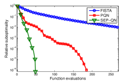
(a) epochs of $\ell_{1}$-logistic regression

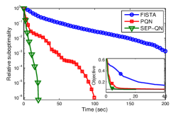
(b) runtime of $\ell_{1}$-logistic regression

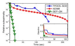
(c) fused $\ell_{1}$-logistic regression

Figure 1: Convergence comparison

We implement all the experiments on a single machine running the 64-bit version of Linux with an Intel Core i5-3470 CPU and 8 GB RAM. We test the SEP-QN framework on various real-world datasets such as gisette ($n=6,000$ and $p=5,000$) and epsilon ($n=300,000$ and $p=2,000$) which can be downloaded from LIBSVM website. The dataset characteristics are provided in the Table 1.

Table 1: Details of the datasets in our experiments

Dataset	p	n (train)	n (test)	nnz (train)
epsilon	2,000	300,000	100,000	600,000,000
gisette	5,000	6,000	1,000	29,729,997
usps	649	1000	1000	649,000

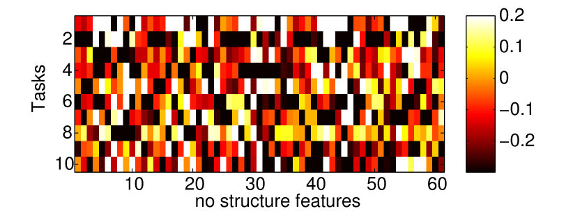
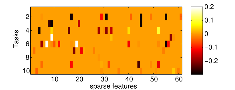
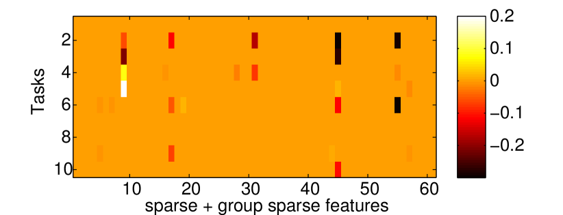
Figure 2: Feature visualization. As shown in the colorbar, orange color indicates that the value of corresponding feature is 0.

“Superposition-structured” Logistic Regression

We consider the “superposition-structured” logistic regression problem:

$$\underset{\mathbf{x}\in\mathbb{R}^{p}}{\min}\;\frac{1}{n}\sum_{i=1}^{n}{\log}(1+{\exp}(-y_{i}{\bf a}_{i}^{T}\mathbf{x}))+\lambda\|\mathbf{x}\|_{1}+\gamma\|\mathbf{W}\mathbf{x}\|_{q}.$$

We first set $\mathbf{W}=\mathbf{0}$ for comparison with the result of PQN in (?). For fairness of comparison, we use the same dataset gisette and the same setting of the tuning parameter $\lambda$ as (?; ?). The results are shown in the Figures 1(a) and 1(b). We can see that the SEP-QN method has the fastest convergence rate, which agrees with Theorems 3 and 3.

In order to verify the effectiveness and efficiency when the model has multiple structural constraints.We compare SEP-QN with ADMM and the direct SCD in TFOCS (?) on the fused sparse logistic regression by setting $\|\mathbf{W}\mathbf{x}\|_{q}=\|\mathbf{x}\|_{TV}$ and $\gamma=\lambda$. Figure 1(c) shows that the three algorithms converge to the same optimal value, but SEP-QN performs much better.

Table 2: The comparisons on multi-task problems.

n	relative error	sparse + group sparse (test error rate / training time )			Other Models
		SEP-QN	QUIC & DIRTY	ADMM	Lasso	Group Lasso
100	$10^{-1}$	7.3% / 0.32s	8.3% / 0.42s	8.3% / 1.5s	7.9%	7.4%
	$10^{-4}$	6.4% / 0.93s	7.4% / 0.75s	7.5% / 4.3s
400	$10^{-1}$	3.0% / 1.2s	2.9% / 1.01s	3.0% / 3.6s	3.0%	3.1%
	$10^{-4}$	2.6% / 2.0s	2.5% / 1.55s	2.6% / 11.0s

(a) feature-number scalability

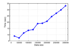
(b) data-size scalability

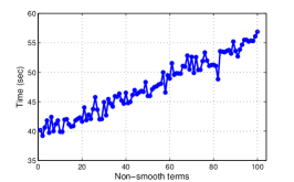
(c) nonsmooth-terms extensibility

Figure 3: Scalability and extensibility

Multi-task Learning

Next we solve the multi-task learning problem where the parameter matrix $\mathbf{X}$ will have a sparse + group sparse structure. In our framework, there is no need to seperate the parameter matrix $\mathbf{X}$ into $\mathbf{S}+\mathbf{B}$ as in (?; ?). Instead of using the square loss (as in (?)), we consider the logistic loss, which gives better performance. Thus, $\mathbf{X}$ could be estimated by the following objective function,

$$\min_{\mathbf{X}\in\mathbb{R}^{p\times r}}\sum_{k=1}^{r}l_{logistic}(\mathbf{y}^{(k)},\mathbf{A}^{(k)}\mathbf{X}^{(k)})+\lambda\|\mathbf{X}\|_{1}+\gamma\|\mathbf{X}\|_{1,2}.$$

We follow (?; ?) and transform multi-class problems into multi-task problems. For fairness of comparison, we test on the same dataset USPS which was first collected in (?) and subsequently widely used in multi-task papers as a reliable dataset for handwritten recognition algorithms. There are $r=10$ tasks, and each handwritten sample consists of $p=649$ features. In (?; ?), the authors demonstrated that on USPS, using sparse and group sparse regularizations together outperforms the models with a single regularizer.

We visualize features that estimated by our SEP-QN framework in Figure 2, and we just plot the first sixty features to provide a clear visualization. Figure 2 shows that the feature structure is well maintained by the regularizer. The promising results of “sparse + group sparse structure” further validate the effectiveness of our SEP-QN framework. As shown in Table 2, our SEP-QN framework is comparable to QUIC & DIRTY which is the state-of-art method. Unlike QUIS & DIRTY, our implementation is straightforward in the SEP-QN framework. Because of broad interest of our framework, it may be slower than QUIC & DIRTY on some specifical datasets. However, we will show that our framework is scalable by the experiments in the following section.

Scalability and Extensibility

We consider the group generalized lasso problem (?; ?; ?), but use the logistic loss function instead for classification. Specifically,

$$\underset{\mathbf{x}\in\mathbb{R}^{p}}{\min} \;\frac{1}{n}\sum_{i=1}^{n}{\log}(1+{\exp}(-y_{i}{\bf a}_{i}^{T}\mathbf{x}))$$

$$+\lambda_{1}\|\mathbf{x}\|_{1}+\lambda_{2}\|\mathbf{F}\mathbf{x}\|_{1}+\sum_{j=1}^{N-2}\gamma_{j}\|\mathbf{G}_{j}\mathbf{x}\|_{2}.$$

As far as we know, there is no an efficient algorithm to solve this model. Note that this dirty model may not be a good choice for gisette and epsilon datasets. We just use this model to validate the scalability and extensibility of SEP-QN framework.

We use the fused sparse logistic regression ($\lambda_{1}=\frac{2}{n},\lambda_{2}=\frac{2}{n},N=2$) and gisette dataset to test the feature-number scalability of SEP-QN as shown in Figure 3(a). Then we test the data-size scalability on epsilon dataset as shown in Figure 3(b). We can see that the convergence time is linear with respect to the number of features as well as the amount of data.

Then we use the group sparse logistic model ($\lambda_{1}=\frac{2}{n},\lambda_{2}=0,\gamma_{j}=\frac{2}{n}$) and epsilon dataset to test the nonsmooth-terms extensibility of SEP-QN. As shown in Figure 3(c), the convergence time is linear with respect to the number of non-smooth terms. These experiments further verify Remark 4 under the assumptions.

5 Conclusion

In this paper, we have generalized the proximal quasi-Newton method to handle “superposition-structured” statistical models and devised a SEP-QN framework. With the help of the SCD approach and LBFGS updating formula, we can solve the surrogate problem in an efficient and feasible way. We have explored the global convergence and the super-linear convergence both theoretically and empirically. Compared with prior methods, SEP-QN converges significantly faster and scales much better, and the promising experimental results on several real-world datasets have further validated the scalability and extensibility of the SEP-QN framework.

Appendix A

Proof of Theorem 2

Lemma A.1.

If  $\mathbf{H}_{k}$ is positive definite, then $\Delta\mathbf{x}_{k}$ satisfies

$$\nabla g(\mathbf{x}_{k})^{T}\Delta\mathbf{x}_{k}+\Psi(\mathbf{x}_{k}+\Delta\mathbf{x}_{k})-\Psi(\mathbf{x}_{k})\leq-\Delta\mathbf{x}_{k}^{T}\mathbf{H}_{k}\Delta\mathbf{x}_{k}$$

The proof of this lemma is shown in (?).

*

Proof.

By Lemma A.1, we have

$$\nabla g(\mathbf{x}_{k})^{T}\Delta\mathbf{x}_{k}+\Psi(\mathbf{x}_{k}+\Delta\mathbf{x}_{k})-\Psi(\mathbf{x}_{k})+\frac{1}{2}\Delta\mathbf{x}_{k}^{T}\mathbf{H}_{k}\Delta\mathbf{x}_{k}$$

$$\leq-\frac{1}{2}\Delta\mathbf{x}_{k}^{T}\mathbf{H}_{k}\Delta\mathbf{x}_{k}\leq 0.$$

Since $\gamma_{k}=\nabla g(\mathbf{x}_{k})^{T}\Delta\mathbf{x}_{k}+\Psi(\mathbf{x}_{k}+\Delta\mathbf{x}_{k})-\Psi(\mathbf{x}_{k})$ (the sufficient descent condition (5)), we have

$$\nabla g(\mathbf{x}_{k})^{T}\Delta\mathbf{x}_{k}+\Psi(\mathbf{x}_{k}+\Delta\mathbf{x}_{k})-\Psi(\mathbf{x}_{k})+\frac{1-\alpha}{2}\Delta\mathbf{x}_{k}^{T}\mathbf{H}_{k}\Delta\mathbf{x}_{k}$$

$$\leq\alpha\gamma_{k}$$

$$g(\mathbf{x}_{k})+\nabla g(\mathbf{x}_{k})^{T}\Delta\mathbf{x}_{k}+\Psi(\mathbf{x}_{k}+\Delta\mathbf{x}_{k})+\frac{1-\alpha}{2}\Delta\mathbf{x}_{k}^{T}\mathbf{H}_{k}\Delta\mathbf{x}_{k}$$

$$\leq g(\mathbf{x}_{k})+\Psi(\mathbf{x}_{k})+\alpha\gamma_{k}.$$ (A.1)

Since $\nabla^{2}g$ is Lipschitz continuous with constant $L_{2}$, the smooth part $g(x)$ can be expanded in Taylor’s series as following

$$f(\mathbf{x}_{k}+\Delta\mathbf{x}_{k}) =g(\mathbf{x}_{k})+\nabla g(\mathbf{x}_{k})^{T}\Delta\mathbf{x}_{k}+\frac{1}{2}\Delta\mathbf{x}_{k}^{T}\nabla^{2}g(\mathbf{x}_{k})\Delta\mathbf{x}_{k}$$

$$+o(\Delta\mathbf{x}_{k}^{2})+\Psi(\mathbf{x}_{k}+\Delta\mathbf{x}_{k})$$

$$\leq g(\mathbf{x}_{k})+\nabla g(\mathbf{x}_{k})^{T}\Delta\mathbf{x}_{k}+\frac{1}{2}\Delta\mathbf{x}_{k}^{T}\nabla^{2}g(\mathbf{x}_{k})\Delta\mathbf{x}_{k}$$

$$+\frac{L_{2}}{6}\|\Delta\mathbf{x}_{k}\|_{2}^{3}+\Psi(\mathbf{x}_{k}+\Delta\mathbf{x}_{k}).$$ (A.2)

Since $\mathbf{H}_{k}\succcurlyeq m\mathbf{I}$, from Lemma A.1, we have

$$\|\Delta\mathbf{x}_{k}\|_{2}^{2}\leq-\frac{\gamma_{k}}{m}.$$ (A.3)

Because $(1-\alpha)\mathbf{H}_{k}\succ\nabla^{2}g(\mathbf{x}_{k})$, we use the results in (A), (A) and (A.3) to yield

$$f(\mathbf{x}_{k}+\Delta\mathbf{x}_{k}) \leq g(\mathbf{x}_{k})+\nabla g(\mathbf{x}_{k})^{T}\Delta\mathbf{x}_{k}+\Psi(\mathbf{x}_{k}+\Delta\mathbf{x}_{k})+$$

$$\frac{1-\alpha}{2}\Delta\mathbf{x}_{k}^{T}\mathbf{H}_{k}\Delta\mathbf{x}_{k}+\frac{L_{2}}{6}\|\Delta\mathbf{x}_{k}\|_{2}^{3}$$

$$\leq f(\mathbf{x}_{k})+\alpha\gamma_{k}+\frac{L_{2}}{6}\|\Delta\mathbf{x}_{k}\|_{2}^{3}$$

$$\leq f(\mathbf{x}_{k})+\alpha\gamma_{k}-\frac{L_{2}}{6m}\|\Delta\mathbf{x}_{k}\|_{2}\gamma_{k}.$$

We can show that $\|\Delta\mathbf{x}_{k}\|_{2}$ converges to zero via Theorem 3. Hence, for $k$ sufficiently large, the unit step length satisfies the sufficient descent condition (5). ∎

Proof of Theorem 2

*

Proof.

By assumptions $\mathbf{s}_{k}^{T}\mathbf{y}_{k}>0$ and $H_{0}\succ\mathbf{0}$, we can prove this result using the BFGS updating formula,

$$\mathbf{H}_{k+1}^{-1}=(\mathbf{I}-\frac{\mathbf{s}_{k}\mathbf{y}_{k}^{T}}{\mathbf{y}_{k}^{T}\mathbf{s}_{k}})\mathbf{H}_{k}^{-1}(\mathbf{I}-\frac{\mathbf{y}_{k}\mathbf{s}_{k}^{T}}{\mathbf{y}_{k}^{T}\mathbf{s}_{k}})+\frac{\mathbf{s}_{k}\mathbf{s}_{k}^{T}}{\mathbf{y}_{k}^{T}\mathbf{s}_{k}}.$$

By reduction, if $\mathbf{H}_{k}^{a}\succ\mathbf{H}_{k}^{b}\succ\mathbf{0}$,

$$(\mathbf{H}_{k+1}^{b})^{-1}-(\mathbf{H}_{k+1}^{a})^{-1}=(\mathbf{I}-\frac{\mathbf{s}_{k}\mathbf{y}_{k}^{T}}{\mathbf{y}_{k}^{T}\mathbf{s}_{k}})((\mathbf{H}_{k}^{b})^{-1}-(\mathbf{H}_{k}^{a})^{-1})(\mathbf{I}-\frac{\mathbf{y}_{k}\mathbf{s}_{k}^{T}}{\mathbf{y}_{k}^{T}\mathbf{s}_{k}})$$

is positive definite when $\mathbf{s}_{k}^{T}\mathbf{y}_{k}>0$, then $\mathbf{H}_{k+1}^{a}\succ\mathbf{H}_{k+1}^{b}$, so with larger initial $\mathbf{H}_{0}$, we could obtain larger $\mathbf{H}_{k}$. ∎

Proof of Theorem 3

Lemma A.2.

Suppose $f$ is a closed convex function and $\underset{\mathbf{x}}{\inf}\{f(\mathbf{x})|\mathbf{x}\in\mathrm{dom}f\}$ is attained at some $\mathbf{x}^{*}$, If $\mathbf{H}_{k}\succ l\mathbf{I}$ for some $l>0$ and the surrogate problem (3) is solved exactly in proximal quasi-Newton method, then $\mathbf{x}_{k}$ converges to an optimal solution starting at any $\mathbf{x}_{0}\in\mathrm{dom}f$.

The proof of this Lemma is shown in (?). *

Proof.

From Algorithm 2, SEP-QN use SCD to solve the local proximal of the composite functions, and the adaptive Hessian strategy keep $\mathbf{H}_{k}\succ l\mathbf{I}$  for some $l>0$. By continuation SCD, the surrogate problem (3) would be solved exactly. Based on Lemma A.2 and Assumption 1, $\mathbf{x}_{k}$ converges to an optimal solution $\mathbf{x}^{*}$ starting at any $\mathbf{x}_{0}\in\mathrm{dom}f$. ∎

Proof of Theorem 3

*

Proof.

After sufficiently many iterations, $\beta\approx 1$. Under the Dennis-More criterion, we can show that the unit step length satisfied the sufficient descent condition (5) via the argument used in the proof of Theorem 2. Then we have,

$$\|Vx_{k+1}-\mathbf{x}^{*}\|_{2} =\|\mathbf{x}_{k}+\Delta\mathbf{x}_{k}-\mathbf{x}^{*}\|_{2}$$

$$=\|\mathbf{x}_{k}+\Delta\mathbf{x}_{k}+\Delta\mathbf{x}_{k}^{nt}-\Delta\mathbf{x}_{k}^{nt}-\mathbf{x}^{*}\|_{2}$$

$$\leq\|\mathbf{x}_{k}+\Delta\mathbf{x}_{k}^{nt}-\mathbf{x}^{*}\|_{2}+\|\Delta\mathbf{x}_{k}-\Delta\mathbf{x}_{k}^{nt}\|_{2}$$ (A.4)

According to Theorem 3.4 in (?), the proximal Newton method convergence quadraticly, that is,

$$\|\mathbf{x}_{k+1}^{nt}-\mathbf{x}^{*}\|_{2} \leq\frac{L_{2}}{2l}\|\mathbf{x}_{k}^{nt}-\mathbf{x}^{*}\|_{2}^{2}$$ (A.5)

By continuation SCD, the surrogate problem (3) would be solved exactly. We draw the same conclusion as (?), that is,

$$\|\Delta\mathbf{x}_{k}-\Delta\mathbf{x}_{k}^{nt}\|_{2}\leq c_{1}\|\mathbf{x}_{k}-\mathbf{x}^{*}\|_{2}^{\frac{1}{2}}\|\Delta\mathbf{x}_{k}\|_{2}+o(\|\Delta\mathbf{x}_{k}\|_{2})$$

$$\|\Delta\mathbf{x}_{k}\|_{2}\leq c_{2}\|\Delta\mathbf{x}^{nt}\|_{2}=c_{2}\|\mathbf{x}_{k+1}^{nt}-\mathbf{x}_{k}\|_{2}$$

$$\leq O(\|\mathbf{x}_{k}-\mathbf{x}^{*}\|_{2}^{2})+c_{2}(\|\mathbf{x}_{k}-\mathbf{x}^{*}\|_{2})$$ (A.6)

From (A), (A.5) and (A), we conclude that,

$$\|\mathbf{x}_{k+1}-\mathbf{x}^{*}\|_{2} \leq\frac{L_{2}}{2l}\|\mathbf{x}_{k}^{nt}-\mathbf{x}^{*}\|_{2}^{2}+o(\|\mathbf{x}_{k}-\mathbf{x}^{*}\|_{2}).$$

Because proximal Newton method convergence much quickly, we deduce that $\mathbf{x}_{k}$ converges to $\mathbf{x}^{*}$ superlinearly. ∎

References

- [Auslender and Teboulle 2006] Auslender, A., and Teboulle, M. 2006. Interior gradient and proximal methods for convex and conic optimization. SIAM Journal on Optimization 16(3):697–725.
- [Beck and Teboulle 2009] Beck, A., and Teboulle, M. 2009. A fast iterative shrinkage-thresholding algorithm for linear inverse problems. SIAM Journal on Imaging Sciences 2(1):183–202.
- [Becker and Fadili 2012] Becker, S., and Fadili, J. 2012. A quasi-Newton proximal splitting method. In Advances in Neural Information Processing Systems, 2618–2626.
- [Becker, Candès, and Grant 2012] Becker, S.; Candès, E.; and Grant, M. 2012. TFOCS: Templates for first-order conic solvers.
- [Boyd et al. 2011] Boyd, S.; Parikh, N.; Chu, E.; Peleato, B.; and Eckstein, J. 2011. Distributed optimization and statistical learning via the alternating direction method of multipliers. Foundations and Trends® in Machine Learning 3(1):1–122.
- [Chandrasekaran et al. 2010] Chandrasekaran, V.; Parrilo, P.; Willsky, A. S.; et al. 2010. Latent variable graphical model selection via convex optimization. In Communication, Control, and Computing (Allerton), 2010 48th Annual Allerton Conference on, 1610–1613. IEEE.
- [Combettes and Pesquet 2012] Combettes, P. L., and Pesquet, J.-C. 2012. Primal-dual splitting algorithm for solving inclusions with mixtures of composite, Lipschitzian, and parallel-sum type monotone operators. Set-Valued and variational analysis 20(2):307–330.
- [Fan et al. 2008] Fan, R.-E.; Chang, K.-W.; Hsieh, C.-J.; Wang, X.-R.; and Lin, C.-J. 2008. Liblinear: A library for large linear classification. The Journal of Machine Learning Research 9:1871–1874.
- [Friedman, Hastie, and Tibshirani 2009] Friedman, J.; Hastie, T.; and Tibshirani, R. 2009. glmnet: Lasso and elastic-net regularized generalized linear models. R package version 1.
- [Grant and Boyd 2014] Grant, M., and Boyd, S. 2014. CVX: Matlab software for disciplined convex programming, version 2.1.
- [Hsieh et al. 2014] Hsieh, C.-J.; Dhillon, I. S.; Ravikumar, P. K.; Becker, S.; and Olsen, P. A. 2014. QUIC & DIRTY: A quadratic approximation approach for dirty statistical models. In Advances in Neural Information Processing Systems, 2006–2014.
- [Jalali et al. 2010] Jalali, A.; Sanghavi, S.; Ruan, C.; and Ravikumar, P. K. 2010. A dirty model for multi-task learning. In Advances in Neural Information Processing Systems, 964–972.
- [Kim and Xing 2010] Kim, S., and Xing, E. P. 2010. Tree-guided group lasso for multi-task regression with structured sparsity. In Proceedings of the 27th International Conference on Machine Learning (ICML-10), 543–550.
- [Lan, Lu, and Monteiro 2011] Lan, G.; Lu, Z.; and Monteiro, R. D. 2011. Primal-dual first-order methods with iteration-complexity for cone programming. Mathematical Programming 126(1):1–29.
- [Lee, Sun, and Saunders 2012] Lee, J.; Sun, Y.; and Saunders, M. 2012. Proximal Newton-type methods for convex optimization. In Advances in Neural Information Processing Systems, 836–844.
- [Lee, Sun, and Saunders 2014] Lee, J. D.; Sun, Y.; and Saunders, M. A. 2014. Proximal Newton-type methods for minimizing composite functions. SIAM Journal on Optimization 24(3):1420–1443.
- [Meier, Van De Geer, and Bühlmann 2008] Meier, L.; Van De Geer, S.; and Bühlmann, P. 2008. The group lasso for logistic regression. Journal of the Royal Statistical Society: Series B (Statistical Methodology) 70(1):53–71.
- [Nesterov 2005] Nesterov, Y. 2005. Smooth minimization of non-smooth functions. Mathematical programming 103(1):127–152.
- [Nesterov 2007] Nesterov, Y. 2007. Gradient methods for minimizing composite objective function.
- [Nocedal and Wright 2006] Nocedal, J., and Wright, S. 2006. Numerical optimization, series in operations research and financial engineering. Springer, New York, USA.
- [Schmidt, Kim, and Sra 2011] Schmidt, M.; Kim, D.; and Sra, S. 2011. Projected Newton-type methods in machine learning.
- [Simon et al. 2013] Simon, N.; Friedman, J.; Hastie, T.; and Tibshirani, R. 2013. A sparse-group lasso. Journal of Computational and Graphical Statistics 22(2):231–245.
- [Tibshirani et al. 2005] Tibshirani, R.; Saunders, M.; Rosset, S.; Zhu, J.; and Knight, K. 2005. Sparsity and smoothness via the fused lasso. Journal of the Royal Statistical Society: Series B (Statistical Methodology) 67(1):91–108.
- [Tseng 2008] Tseng, P. 2008. On accelerated proximal gradient methods for convex-concave optimization. submitted to SIAM Journal on Optimization.
- [Van Breukelen et al. 1998] Van Breukelen, M.; Duin, R. P.; Tax, D. M.; and Den Hartog, J. 1998. Handwritten digit recognition by combined classifiers. Kybernetika 34(4):381–386.
- [Yang and Ravikumar 2013] Yang, E., and Ravikumar, P. K. 2013. Dirty statistical models. In Advances in Neural Information Processing Systems, 611–619.
- [Yuan, Ho, and Lin 2012] Yuan, G.-X.; Ho, C.-H.; and Lin, C.-J. 2012. An improved glmnet for l1-regularized logistic regression. The Journal of Machine Learning Research 13(1):1999–2030.
- [Zhou et al. 2012] Zhou, J.; Liu, J.; Narayan, V. A.; and Ye, J. 2012. Modeling disease progression via fused sparse group lasso. In Proceedings of the 18th ACM SIGKDD international conference on Knowledge discovery and data mining, 1095–1103. ACM.