On Capacity Formulation with Stationary Inputs and Application to a Bit-Patterned Media Recording Channel Model

Abstract

In this correspondence, we illustrate among other things the use of the stationarity property of the set of capacity-achieving inputs in capacity calculations. In particular, as a case study, we consider a bit-patterned media recording channel model and formulate new lower and upper bounds on its capacity that yield improvements over existing results. Inspired by the observation that the new bounds are tight at low noise levels, we also characterize the capacity of this model as a series expansion in the low-noise regime.

The key to these results is the realization of stationarity in the supremizing input set in the capacity formula. While the property is prevalent in capacity formulations in the ergodic-theoretic literature, we show that this realization is possible in the Shannon-theoretic framework where a channel is defined as a sequence of finite-dimensional conditional probabilities, by defining a new class of consistent stationary and ergodic channels.

I Background

The fundamental limit of information transmission through noisy channels, the channel capacity, has been a holy grail in information theory. The capacity problem of a general point-to-point channel has been well resolved with the information-spectrum framework [1]. Such general formula for the capacity, however, does not lend itself to computation in general, since it requires one to scrutinize the distribution of the information density at the limit of infinite block length. To overcome this problem, a common approach is to find an alternative expression that, instead of being described by an information-spectrum quantity, contains a mutual information quantity (or entropy quantities). While an expression of this kind is not as general, it may cover a sufficiently large class of channels for many practical purposes.

There are two popular forms of such expression. One is Dobrushin's information-stable channel capacity [2]:

$$C=\lim_{n\to\infty}\frac{1}{n}\sup_{X^{n}}I\left(X^{n};Y^{n}\right)$$ (1)

where the supremum is over all possible sequences of distributions $\left\{P^{\left(n\right)}:\;X^{n}\sim P^{\left(n\right)}\right\}$. This formula holds for the class of information-stable channels. A similar formula also appears in the context of (decomposable or indecomposable) finite-state channels [3]. The other form swaps the supremum and the limit in the above formula, with the supremum being taken over a smaller set of input distributions with special structures. This type of formula appears in the ergodic-theoretic literature of information theory. For example, for $\bar{d}$-continuous discrete stationary and ergodic (SE) two-sided channels, the capacity was shown to be [4]

$$C=\sup_{\text{Stationary }\mu}\lim_{n\to\infty}\frac{1}{n}I\left(X^{n};Y^{n}\right)$$ (2)

where $\mu$ is a probability measure that describes the input process. (See Section I-B for the distinction between the two sets being supremized over in the above formulas.)

Such capacity formulations that involve supremization over stationary inputs are common in the ergodic-theoretic setting, where a channel only admits infinitely long input sequences, mostly for SE channels with memory and anticipation [5, 4]. In the Shannon-theoretic framework, where an admissible input is a sequence of finite-dimensional distributions, capacity formulations similar to Eq. (1) are, however, more prevalent.

Intuitively constraints on the supremizing input set reduce the capacity-achieving input search space and may become useful. A major aim of this paper is to illustrate possible ways to exploit the stationarity property of the supremizing input set in capacity calculations, via a case study of a bit-patterned media recording (BPMR) channel model. This model was first introduced in [8] and subsequently studied in [9]. To achieve ultra-high density magnetic recording, in BPMR technologies, the data write process takes place on a new magnetic medium comprising of magnetic islands that are separated by non-magnetic materials. The difficulty in maintaining synchronization between the write head's position and the correct island where data is to be written in is captured by a channel model with paired insertion-deletion errors, underlied by a first-order Markov process. The channel input is the actual data to be written and the output is the data as written on the islands. This channel model is essentially a finite-state channel with dependent insertion-deletion (DID) errors, and is henceforth called the DID channel model.

Both works [8] and [9] analyze the capacity of the DID channel using a formula of the form of Eq. (1). In our case study, we will contrast this with the use of a formula that involves stationary inputs, which is able to yield improvements and new results. In particular, the formula we seek assumes a form similar to Eq. (2). We consider both Shannon-theoretic and ergodic-theoretic frameworks. While we analyze specifically the DID channel, we believe techniques we present to evaluate its capacity could be applicable to similar BPMR channel models, e.g. the model in [10], and beyond.

We give a high-level view of the calculation techniques. As in Eq. (1) and (2), computing the capacity generally involves an infinite-dimensional optimization problem, which in most cases is intractable. Our idea towards computational feasibility is to decompose $I\left(X^{n};Y^{n}\right)$ into a sum of finite-dimensional terms of the form

$$I\left(X^{n};Y^{n}\right)\approx\sum_{i=1}^{n}f\left(\left\llbracket X\right\rrbracket_{i},\left\llbracket Y\right\rrbracket_{i},\left\llbracket Z\right\rrbracket_{i}\right)$$

where $\left\llbracket X\right\rrbracket_{i}$ indicates a finite-size group of terms in the neighborhood of $X_{i}$ (i.e. $\left(X_{i-a},X_{i-a+1},\ldots,X_{i+b}\right)$ for some finite non-negative constants $a$ and $b$), and the same for $\left\llbracket Y\right\rrbracket_{i}$ and $\left\llbracket Z\right\rrbracket_{i}$, and $f$ is a function mapping the joint distribution of $\left(\left\llbracket X\right\rrbracket_{i},\left\llbracket Y\right\rrbracket_{i},\left\llbracket Z\right\rrbracket_{i}\right)$ to $\mathbb{R}_{+}$ and is independent of the index $i$. Here $\left\llbracket Z\right\rrbracket_{i}$ can be thought of as an external source of randomness introduced by the channel. The approximation ``$\approx$'' is to be replaced with an exact inequality (i.e. ``$\leq$'' or ``$\geq$''). Given the finite-dimensional distribution of each input block $\left\llbracket X\right\rrbracket_{i}$, $f\left(\left\llbracket X\right\rrbracket_{i},\left\llbracket Y\right\rrbracket_{i},\left\llbracket Z\right\rrbracket_{i}\right)$ can be computed. However the curse of dimensionality is not yet completely eliminated: for a general input, we have $n$ possibly different distributions for $\left\llbracket X\right\rrbracket_{1},\left\llbracket X\right\rrbracket_{2},\ldots,\left\llbracket X\right\rrbracket_{n}$.

The problem is resolved when the input is stationary, in which we reduce the number of said distributions from $n$ to one, which is the lowest possible. Furthermore, for many classes of channels, input stationarity implies stationarity of $\left\{\left\llbracket X\right\rrbracket_{i},\left\llbracket Y\right\rrbracket_{i},\left\llbracket Z\right\rrbracket_{i}\right\}_{i=1}^{n}$. Effectively,

$$\frac{1}{n}I\left(X^{n};Y^{n}\right)\approx f\left(\left\llbracket X\right\rrbracket_{i},\left\llbracket Y\right\rrbracket_{i},\left\llbracket Z\right\rrbracket_{i}\right)$$

which is now computable.

Broadly speaking, input stationarity helps reduce an infinite-dimensional problem to a finite-dimensional one. This reduction is potentially useful for constructing upper bounds on the capacity. With a ``good'' $f$, one may hope $f\left(\left\llbracket X\right\rrbracket_{i},\left\llbracket Y\right\rrbracket_{i},\left\llbracket Z\right\rrbracket_{i}\right)$ provides a tight upper bound. With a matching lower bound, the exact capacity can be deduced. We make a note that the advantage is not only computational, but also analytical, since we then only need to work with a finite number of variables, instead of infinitely many. We shall illustrate so for the case of the DID channel.

For the rest of this section, after introducing some mathematical conventions and common definitions, we briefly discussed the two different channel definitions that correspond to the two frameworks, and their relation to practical channel models. We then give a brief description of the DID channel model with known results on its capacity and outline the main contributions of the paper.

I-A Mathematical Conventions

To denote random variables, uppercase letters (e.g. $V$, $X$, $Y$) are used, and corresponding lowercase letters (e.g. $v$, $x$, $y$) are adopted for values they take. Their respective alphabets are in calligraphic style (e.g. $\mathcal{V}$, $\mathcal{X}$, $\mathcal{Y}$). $V_{a}^{b}$ denotes the vector $\left(V_{a},V_{a+1},...,V_{b}\right)^{\top}$ for $a\leq b$. At times $V^{b}$ may be used in place of $V_{1}^{b}$ (or $V_{0}^{b}$ where appropriate). Whenever the length is not specified or is implicitly understood, the vector is written in boldface, e.g. $\mathbf{V}$ (resp. $\mathbf{v}$), in which case $V_{a}$ (resp. $v_{a}$) denotes its $a$-th entry. All vectors are understood to be column vectors.

The notation $\left\{V_{i}\right\}_{i=1}^{\infty}$ (or $\left\{V_{i}\right\}$, depending on the starting index) denotes a one-sided random process. We only consider processes $\left\{V_{i}\right\}$ in which $V_{i}\in\mathcal{V}$ $\forall i$. This restriction is technically not an issue, since we can always expand the alphabet of each $V_{i}$ to the largest one, with an appropriately modified probability measure that assigns probability $0$ to any event that involves taking values that are not in the original alphabets.

An event $E_{V}$ (on a process $\left\{V_{i}\right\}$) is a set of values $\mathbf{v}$ that the process takes. At times we use the notations, e.g. $\left\{V_{i}=a\right\}$, to refer to an event $\left\{\mathbf{v}:\;v_{i}=a\right\}$. A similar meaning applies to e.g. $\left\{V_{i}=a\;\text{or}\;V_{i}=b\right\}$. We also write e.g. $\left\{V_{a}^{a+b}=v_{1}v_{2}...v_{b+1}\right\}$, where $v_{1},v_{2},...,v_{b+1}\in{\cal V}$, to mean $\left\{V_{a}=v_{1},V_{a+1}=v_{2},...,V_{a+b}=v_{b+1}\right\}$.

The letter $X$ is used specifically for the channel input, and the letter $Y$ is for the channel output.

The operator $\left|\cdot\right|$ returns the length of a vector, e.g. $\left|V_{a}^{b}\right|=b-a+1$, the absolute value of a scalar quantity, or the size of a set. The expectation operator is $\mathbb{E}\left[\cdot\right]$. The binary entropy function is $h_{2}(x)=-x\log x-(1-x)\log(1-x)$. We write $\left[\mathbf{x},\mathbf{y}\right]$ to denote the concatenation of vectors $\mathbf{x}$ and $\mathbf{y}$, i.e. $\left[\mathbf{x},\mathbf{y}\right]=\left(x_{1},...,x_{\left|\mathbf{x}\right|},y_{1},...,y_{\left|\mathbf{y}\right|}\right)^{\top}$. When the alphabet is binary, we use $\neg\mathbf{x}$ to denote the vector obtained by flipping all bits in $\mathbf{x}$, and $\neg E$ to denote $\left\{\neg\mathbf{x}:\;\mathbf{x}\in E\right\}$.

Throughout this paper, $\log$ is understood to be of base $2$.

I-B Definitions

Let $T$ denote the left-shift transformation. That is, e.g. for a vector $\left(v_{1},v_{2},...\right)^{\top}$, we have $T\left(v_{1},v_{2},...\right)^{\top}=\left(v_{2},v_{3},...\right)^{\top}$. Also, let $T^{-1}E=\left\{\mathbf{v}:\;T\mathbf{v}\in E\right\}$.

We refer to ``finite-dimensional'' events as cylinders. That is, a cylinder $E$ on the process $\{V_{n}\}_{n=1}^{\infty}$ takes the form $c_{t}^{m}\left(G\right)=\left\{\mathbf{v}:\;\left(v_{t},v_{t+1},\ldots,v_{t+m-1}\right)\in G\right\}$ for some $G\subseteq{\cal V}^{m}$. Also, $\text{cylind}\left(t,m,{\cal V}\right)=\left\{c_{t}^{m}\left(G\right):\;G\subseteq{\cal V}^{m}\right\}$, the set of all cylinders with ``starting index'' $t$ and length $m$ over ${\cal V}$. For finite $m$ and ${\cal V}$, $\text{cylind}\left(t,m,{\cal V}\right)$ is finite-sized.

A random process $\left\{V_{n}\right\}$, defined over a probability space $\left(\Omega,\mathcal{F},P\right)$, is said to be stationary if $\forall E\in\mathcal{F}$, $P\left(E\right)=P\left(T^{-1}E\right)$. It is $N$-stationary, for some integer $N\geq 1$, if $\forall E\in\mathcal{F}$, $P\left(E\right)=P\left(T^{-N}E\right)$. It is ergodic if $P\left(E\right)=0$ or $P\left(E\right)=1$ for all invariant events $E\in\mathcal{F}$.

The notion of stationarity can be extended to an $n$-dimensional probability measure $P^{\left(n\right)}$ for finite $n$. That is,

$$P^{\left(n\right)}\left(E\times{\cal V}\right)=P^{\left(n\right)}\left(T^{-1}E\right)\quad\forall E\subseteq{\cal V}^{n-1}$$

It can be observed that if $P$ is stationary and $P^{\left(n\right)}$ is an $n$-dimensional marginal of $P$, i.e. $P^{\left(n\right)}\left(E\right)=P\left(\left\{V_{1+k}^{n+k}\in E\right\}\right)$ $\forall E\subseteq{\cal V}^{n}$ for some $k$, then $P^{\left(n\right)}$ is stationary.

We make a note on Kolmogorov consistency. A sequence $\left\{V^{n}\right\}$ is consistent, where $V^{n}$ is associated with probability measure $P^{\left(n\right)}$ for each $n$, if

$$\sum_{v_{n+1}\in{\cal V}}P^{\left(n+1\right)}\left(v^{n+1}\right)=P^{\left(n\right)}\left(v^{n}\right)\quad\forall v^{n}\in{\cal V}^{n}$$

for every $n$. That is, consistent $\left\{V^{n}\right\}$ can be described by a single probability measure, whereas inconsistent $\left\{V^{n}\right\}$ is described by an infinite number of probability measures $\left\{P^{\left(n\right)}\right\}$. Notice that the notation $\left\{V_{n}\right\}$ implies a standard random process which must be consistent by definition, while $\left\{V^{n}\right\}$ is only a sequence in $n$. The two notations coincide if $\left\{V^{n}\right\}$ is consistent. We also note that if $\left\{V^{n}\right\}$ is stationary, $N$-stationary or ergodic, it must be specified by a single probability measure and therefore consistent.

I-B1 Channel Definitions

We discuss the channel definition in two settings: the ergodic-theoretic framework (see e.g. [5]) and the Shannon-theoretic framework (see e.g. [1]).

• In the ergodic-theoretic setting, a channel is defined as a list of probability measures $\left\{\nu_{\mathbf{x}}:\;\mathbf{x}\in{\cal X}^{\infty}\right\}$ which act on output events $E_{Y}\subseteq{\cal Y}^{\infty}$, where each $\mathbf{x}$ is either a bi-infinite sequence (i.e. $\mathbf{x}=\left(\ldots,x_{-1},x_{0},x_{1},\ldots\right)$) or a uni-infinite sequence (i.e. $\mathbf{x}=\left(x_{k},x_{k+1},\ldots\right)$ for some finite $k\in\mathbb{Z}$). This definition only admits inputs that are consistent random processes. The joint input-output distribution $\omega$ for an input process $\mu$ is determined by

  $$\omega\left(E_{X},E_{Y}\right)=\int_{E_{X}}\nu_{\mathbf{x}}\left(E_{Y}\right)d\mu\left(\mathbf{x}\right)$$ (3)

  for any events $E_{X}$ and $E_{Y}$ on the channel input and output respectively. Here we only consider uni-infinite input sequences only, which correspond to one-sided processes and one-sided channels. The literature on bi-infinite inputs (and correspondingly two-sided channels) is more extensive, but lacks the descriptive power for the channel model of application in this paper, i.e. the DID channel.

• The Shannon-theoretic definition of a channel is a sequence of finite-dimensional conditional probability measures $\left\{P_{\left.\mathbf{Y}\middle|X^{n}\right.}\left(\cdot\middle|\mathbf{x}\right),\;\mathbf{x}\in\mathcal{X}^{n}\right\}_{n=1}^{\infty}$, in which $\mathbf{Y}$ can take any abstract alphabet. This definition avoids placing any restrictions on the channel and allows inputs that are not necessarily consistent and take the form $\left\{X^{n}\right\}$. The joint input-output distribution is determined for each block length $n$, i.e.

  $$P_{X^{n}\mathbf{Y}}\left(x^{n},\mathbf{y}\right)=P_{\left.\mathbf{Y}\middle|X^{n}\right.}\left(\mathbf{y}\middle|x^{n}\right)Q^{\left(n\right)}\left(x^{n}\right)$$ (4)

  where $X^{n}\sim Q^{\left(n\right)}$, and it is not necessarily consistent throughout all $n$'s.

Compatibility between the two definitions may not be entirely immediate. On one hand, the sequence in the Shannon-theoretic definition may not be viewed as converging to a limit equal to the ergodic-theoretic definition without careful justification of such a limit. On the other hand, the lack of channel laws $P_{\left.\mathbf{Y}\middle|X^{n}\right.}\left(\cdot\middle|\mathbf{x}\right)$ for finite block lengths $n$ in the ergodic-theoretic framework has been noted to pose technical difficulties in proving coding theorems [4]. The difference in the channel definition, as noted in [1], also leads to a difference in how the error probability is defined. Despite this discrepancy, the capacities under the two frameworks are of little difference in the overall implication to reliable communications in the asymptotic regime of infinite block length. Depending on the actual channel model, one may find either framework suitable. In general, we shall treat the two frameworks separately.

I-B2 From Channel Definitions to Channel Models

The channel definitions abstract away from specific channel models and form the basis under which reliable communications is defined. Practical channel models, however, are usually not described in terms of probability measures as in the channel definitions. When the ergodic-theoretic channel definition is applicable to a channel model, we mean that there exists a list of probability measures $\left\{\nu_{\mathbf{x}}:\;\mathbf{x}\in{\cal X}^{\infty}\right\}$ such that for every consistent input, the joint input-output distribution can be described by Eq. (3). Likewise, when the Shannon-theoretic channel definition is applicable to a channel model, there exists a sequence of finite-dimensional conditional probability measures $\left\{P_{\left.\mathbf{Y}\middle|X^{n}\right.}\left(\cdot\middle|\mathbf{x}\right),\;\mathbf{x}\in\mathcal{X}^{n}\right\}_{n=1}^{\infty}$ such that for every input $\left\{X^{n}\sim Q^{\left(n\right)}\right\}$, the joint input-output distributions can be described by Eq. (4).

While the two frameworks associated with the two channel definitions are handled separately, when both channel definitions are applicable, the observation that the measures $\nu_{\mathbf{x}}$ and $P_{\left.\mathbf{Y}\middle|X^{n}\right.}\left(\cdot\middle|\mathbf{x}\right)$ coexist for a channel model can be exploited. In particular, in such cases, the joint input-output distribution can be described either ways, thereby allowing certain results from one framework to be used in another.

I-C DID Channel Model

The DID channel model is described by

$$Y_{i}=X_{i-Z_{i}}$$

where $\left\{Z_{i}\right\}_{i=1}^{\infty}$ is a first-order binary Markov process, independent of the binary input. Note that the starting indices of the state process and the output are $1$ and that of the input is $0$. Here $P\left(Z_{i}=1\middle|Z_{i-1}=0\right)=p_{i}$, the insertion probability, and $P\left(Z_{i}=0\middle|Z_{i-1}=1\right)=p_{d}$, the deletion probability.

An illustration is given in Fig. 1. It could be observed that every insertion must be followed by a deletion and vice versa, i.e. insertions and deletions are paired; hence the name dependent insertion-deletion channel.

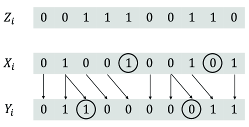
Figure 1: An illustration of the DID channel. The circled input bits are deleted, and the circled output bits are inserted. Each $Z_{i}=0\rightarrow Z_{i+1}=1$ transition induces an insertion, in which the inserted bit is the same as the last input bit, whereas each $Z_{i}=1\rightarrow Z_{i+1}=0$ transition induces a deletion.

This channel describes a simplified model for the BPMR write process, capturing certain key features of the errors introduced in this process. As mentioned, the aim of this technology is to achieve ultra-high storage densities, envisioned at $10\text{ Tb/in}^{2}$ and beyond [11]. Conventional magnetic recording media comprise of successive magnetic units, each of which is written with one data bit, represented by the magnetic state of the unit. As the density increases, interference from adjacent units produces graver effects on the magnetic state, hence degrading the reliability of the process and placing a limit on these media. BPMR, as one of the responses to this problem, separates these units with non-magnetic materials in between. However, as another challenge with increasing densities, the write head does not shrink proportionally with the size of each magnetic unit; in fact, it may span over multiple units. Difficulties thereby arise in controlling the position of the write head relative to the units, leading to timing mismatches. There are two typical erroneous scenarios: one is when the write head lags behind the next unit and fails to write the data bit on this unit, and the other is when it advances beyond the intended unit which is hence written with the past data bit. The first error is modeled by the transition $Z_{i-1}=1\to Z_{i}=0$, and the second error corresponds to $Z_{i-1}=0\to Z_{i}=1$.

For more details about the BPMR, see [12, 11, 13, 14]. A more informative justification of the DID channel model can be found in [8, 9]. It has been pointed out that this model does not capture all error types in the BPMR write process, which motivates another channel model in [10]. They are however similar from an information-theoretic perspective. Since this paper concerns with the capacity aspect of these channels, the simplicity of the DID channel is appealing, making the model suitable for illustrating our information-theoretic results and capacity-evaluating techniques.

A number of bounds on the DID channel capacity have been established in [8] and [9]. In particular, in [8], an upper bound, given by $1-p_{i}p_{d}/\left(p_{i}+p_{d}\right)$ and termed genie-erasure upper bound, was derived, and a numerical simulation-based lower bound, which is in fact the achievable rate $C_{iud}$ with independent and uniformly distributed (i.u.d.) input, was computed for all channel parameters $p_{i}$ and $p_{d}$. The specific case of $p_{d}=1$ was analyzed in [9], which provided a finite-lettered expression of $C_{iud}$ and also the genie-erasure upper bound. However these upper and lower bounds, as seen in [8, Fig. 10, 11] and [9, Fig. 2], are relatively distant. (We reproduce their bounds, plotted as dashed curves, in Fig. 4 and 6 below, for greater convenience of the readers.) We emphasize that both works relied on the capacity formula for indecomposable channels.

In later sections, we restrict our attention to $p_{i}\in(0,1)$ and $p_{d}\in(0,1)$. A simple continuity argument yields results for special cases where $p_{i}\in\{0,1\}$ or $p_{d}\in\{0,1\}$. Henceforth we say e.g. $p_{d}=1$ to mean $p_{d}$ is very close to $1$.

I-D Summary of Contributions and Structure

As said, a main contribution of this work is the realization of the stationarity condition in the supremizing input set. In Sections II and III, we explore this in capacity formulations for the DID channel model in both ergodic-theoretic and Shannon-theoretic frameworks.

• The ergodic-theoretic literature on such formulation is vast. However to the best of our knowledge, the theory developed for one-sided channels contains solely forward coding theorems, which establish achievability results on the rate [5]. Converse theorems, which concern with inachievability, are unfortunately missing. In Section II, we verify that a ``capacity'' formula is applicable to the DID channel. This formula encompasses other known achievable rate formulas for one-sided channels. For simplicity, we shall refer to this formula as a capacity formula.

• To realize input stationarity in the Shannon-theoretic framework, we introduce new definitions on consistent, stationary and ergodic channels, and prove that SE inputs can achieve the capacity of the finite-alphabet class of these channels in Theorem 11. We also verify its applicability to the DID channel. Note that the formula obtained here is the true capacity. These are done in Section III.

Further towards the aim of computational suitability, a portion of these two sections introduces the notion of bit-symmetry and proves that we can further restrict the input search space to bit-symmetric inputs in Proposition 4 (and to a lesser extent, Proposition 14) when the channel is, in addition, bit-symmetric.

While it is not conclusive whether the ergodic-theoretic formula is the true capacity, it is the same as the one in the Shannon-theoretic framework. Subsequent sections are devoted to evaluations of this single formula. In Section IV, a new lower bound is derived analytically in a finite-lettered computable form. A series of new computation-based upper bounds is formulated in Section V. These bounds are shown to yield improvements over those in [8] and [9] and are tight at low noise levels. Inspired by this observation, we then characterize the DID channel capacity in the low-noise regime in Section VI for the case $p_{i}=p_{d}=p_{id}$, given by

$$C=1-\left[\sum_{k=1}^{\infty}\frac{1}{2^{k+1}}h_{2}\left(\frac{1}{2}+\frac{1}{2}\left(1-2p_{id}\right)^{k}\right)\right]+{\cal O}\left(p_{id}^{2}\right)$$

This characterization is achieved (up to the order of $p_{id}^{2}$) by the i.u.d. input. The paper concludes with Section VII.

As shown in [14], in models that closely mimic the actual BPMR write channel, the occurrence frequency should be almost the same for both insertion and deletion errors. For this reason, while our bounds are formulated for any $p_{i}$ and $p_{d}$, we illustrate the numerical evaluation of the DID channel capacity mostly for the case $p_{i}=p_{d}=p_{id}$. It is also shown in [14] that the occurrence frequency could be as low as $10^{-4}$, which justifies our interest in the low-noise regime.

II Ergodic-Theoretic Capacity Formulation

In this section, we find a ``capacity'' formula that involves stationary inputs for the DID channel under the ergodic-theoretic framework. As a reminder, this formula yields an achievable rate, not the true capacity, and we consider one-sided channels only. Our main reference is the work [5]. We also develop the notion of bit-symmetry in this setting. Roughly speaking, bit-symmetry for binary inputs is the property in which the probability of drawing a binary string $\mathbf{x}$ is equal to the probability of drawing $\neg\mathbf{x}$. Likewise, a bit-symmetric (binary) channel is one in which the posterior probability of the output $\mathbf{y}$ given the input $\mathbf{x}$ is equal to that of $\neg\mathbf{y}$ given $\neg\mathbf{x}$. Intuitively a bit-symmetric channel should attain its capacity for some bit-symmetric inputs. We show that this is true for certain channels.

II-A Ergodic-Theoretic Capacity

We review some definitions under the ergodic-theoretic framework.

• A random process $\{V_{n}\}_{n=1}^{\infty}$, defined over a probability space $(\Omega,\mathcal{F},P)$, is said to be asymptotically mean stationary (AMS) if $\forall E\in\mathcal{F}$, the limit

  $$P_{AMS}\left(E\right)=\lim_{n\to\infty}\frac{1}{n}\sum_{i=0}^{n-1}P\left(T^{-i}E\right)$$

  exists. $P_{AMS}$ is called the stationary mean. A stationary processes is also AMS.

• A channel $\left\{\nu_{\mathbf{x}}:\;\mathbf{x}\in{\cal X}^{\infty}\right\}$ is stationary if $\nu_{\mathbf{x}}\left(T^{-1}E_{Y}\right)=\nu_{T\mathbf{x}}\left(E_{Y}\right)$ for any output event $E_{Y}\subseteq{\cal Y}^{\infty}$. It is known that the joint input-output distribution $\omega$ (and hence the output distribution $\eta\left(E_{Y}\right)=\omega\left({\cal X}^{\infty},E_{Y}\right)$) is stationary given a stationary input $\mu$ and a stationary channel [5, Lemma 9.3.1].

• A channel is said to be AMS if given an AMS input, $\omega$ is also AMS. A stationary channel is also AMS [5, Lemma 9.3.2].

• A stationary (resp. AMS) channel is ergodic if $\omega$ is ergodic, given any stationary (resp. AMS) and ergodic input distribution $\mu$.

Let us first consider stationary channels, in which the developments are more straightforward. In the ergodic-theoretic literature, coding theorems are established for finite-alphabet stationary and ergodic (SE) channels with various assumptions on the channel memory and anticipation. A simple class is the class of finite-input-memory and causal channels. A channel is said to have finite input memory if there exists a natural number $m$ such that for any $n$,

$$\nu_{\mathbf{x}}\left(T^{-n}E_{Y}\right)=\nu_{\hat{\mathbf{x}}}\left(T^{-n}E_{Y}\right)$$

for any $\mathbf{x}$ and $\hat{\mathbf{x}}$ such that $x_{n-m}^{\infty}=\hat{x}_{n-m}^{\infty}$ and any event $E_{Y}$. A channel is causal (or without anticipation) if for any $n$,

$$\nu_{\mathbf{x}}\left(\left\{Y^{n}=y^{n}\right\}\right)=\nu_{\hat{\mathbf{x}}}\left(\left\{Y^{n}=y^{n}\right\}\right)$$

for any $\mathbf{x}$ and $\hat{\mathbf{x}}$ such that $x^{n}=\hat{x}^{n}$ and any $y^{n}$.

For the DID channel, we use $P_{X_{0}^{\infty}}$, $P_{X_{0}^{\infty}\mathbf{Y}}$ and $P_{\left.\mathbf{Y}\middle|X_{0}^{\infty}\right.}\left(\cdot\middle|\mathbf{x}\right)$ in place of $\mu$, $\omega$ and $\nu_{\mathbf{x}}$ respectively. The model can be described under the ergodic-theoretic channel definition as follows. For an output sequence $\mathbf{Y}=\mathbf{y}$, given an input sequence $X_{0}^{\infty}=\mathbf{x}$, each triplet $\left(y_{i},x_{i},x_{i-1}\right)$ corresponding to the pair $(\mathbf{x},\mathbf{y})$ uniquely determines the occurrence of either one of the four events $\left\{Z_{i}=0\right\}$, $\left\{Z_{i}=1\right\}$, $\left\{Z_{i}=0\;\text{or}\;Z_{i}=1\right\}$ and $\left\{Z_{i}\in\emptyset\right\}$. Let us denote the determined event ${\cal E}\left(Z_{i};y_{i},x_{i},x_{i-1}\right)$. Also, for some output event $E_{Y}$, let us define

$${\cal E}\left(\mathbf{x},E_{Y}\right)=\bigcup_{\mathbf{y}\in E_{Y}}\bigcap_{i=1}^{\infty}{\cal E}\left(Z_{i};y_{i},x_{i},x_{i-1}\right)$$

Then the channel law $P_{\left.\mathbf{Y}\middle|X_{0}^{\infty}\right.}\left(\cdot\middle|\mathbf{x}\right)$ is determined by

$$P_{\left.\mathbf{Y}\middle|X_{0}^{\infty}\right.}\left(E_{Y}\middle|\mathbf{x}\right) =\int_{E_{Y}}dP_{\left.\mathbf{Y}\middle|X_{0}^{\infty}\right.}\left(\mathbf{y}\middle|\mathbf{x}\right)$$

$$=\int_{E_{Y}}dP_{\mathbf{Z}}\left(\bigcap_{i=1}^{\infty}{\cal E}\left(Z_{i};y_{i},x_{i},x_{i-1}\right)\right)$$

$$\stackrel{{\scriptstyle\left(a\right)}}{{=}}P_{\mathbf{Z}}\left({\cal E}\left(\mathbf{x},E_{Y}\right)\right)$$ (5)

where $P_{\mathbf{Z}}$ is the probability measure of the $\left\{Z_{i}\right\}_{i=1}^{\infty}$ process. The step $\left(a\right)$ is by the following reason: ${\cal E}\left(Z_{i};y_{i},x_{i},x_{i-1}\right)$ and ${\cal E}\left(Z_{i};y_{i}^{\prime},x_{i},x_{i-1}\right)$ are disjoint for $y_{i}\neq y_{i}^{\prime}$, so $\bigcap_{i=1}^{\infty}{\cal E}\left(Z_{i};y_{i},x_{i},x_{i-1}\right)$ and $\bigcap_{i=1}^{\infty}{\cal E}\left(Z_{i};y_{i}^{\prime},x_{i},x_{i-1}\right)$ are disjoint for $\mathbf{y}\neq\mathbf{y}^{\prime}$.

It is easy to see that the DID channel model is finite-input-memory and causal. Combining [5, Theorem 12.6.1] and [5, Lemma 12.4.2], the capacity of the DID channel is given by

$$C =\sup_{\text{\emph{\emph{Stationary} }}P_{X_{0}^{\infty}}}\lim_{n\to\infty}\frac{1}{n}I\left(X_{0}^{n};Y_{1}^{n}\right)$$ (6)

$$=\sup_{\text{\emph{\emph{Stationary} }}P_{X_{0}^{\infty}}}\lim_{n\to\infty}\frac{1}{n}\left[H\left(Y^{n}\right)-H\left(Y^{n}\middle|X_{0}^{n}\right)\right]$$ (7)

$$=\sup_{\text{\emph{\emph{Stationary} }}P_{X_{0}^{\infty}}}\Big{[}\lim_{n\rightarrow\infty}H\left(Y_{n}\middle|Y^{n-1}\right)$$

$$\qquad\qquad\qquad\qquad-\lim_{n\rightarrow\infty}H\left(Y_{n}\middle|Y^{n-1},X_{0}^{n}\right)\Big{]}$$

if it could be shown to be SE. The third equation follows from causality of the channel and the fact that the joint input-output distribution is stationary. We note that the starting indices in the formula are chosen to suit the DID channel description, although this is not critical for the following reason. For any finite non-negative $a$ and $b$,

$$I\left(X_{-b}^{n+a};Y_{1}^{n}\right) =I\left(X_{0}^{n};Y_{1}^{n}\right)+I\left(X_{-b}^{-1},X_{n+1}^{n+a};Y_{1}^{n}\middle|X_{0}^{n}\right)$$

$$\leq I\left(X_{0}^{n};Y_{1}^{n}\right)+\left(a+b\right)\log\left|{\cal X}\right|$$

and that $I\left(X_{-b}^{n+a};Y_{1}^{n}\right)\geq I\left(X_{0}^{n};Y_{1}^{n}\right)$. Then:

$$\lim_{n\rightarrow\infty}\frac{1}{n}I\left(X_{0}^{n};Y_{1}^{n}\right)=\lim_{n\rightarrow\infty}\frac{1}{n}I\left(X_{-b}^{n+a};Y_{1}^{n}\right)$$

since $\left(a+b\right)\log\left|{\cal X}\right|$ is finite.

We now argue that the DID channel is stationary under the condition that $\left\{Z_{i}\right\}_{i=1}^{\infty}$ is stationary, which can be achieved with a suitable initialization: $P\left(Z_{1}=0\right)=p_{d}/\left(p_{i}+p_{d}\right)$ and $P\left(Z_{1}=1\right)=p_{i}/\left(p_{i}+p_{d}\right)$. For any output event $E_{Y}$,

$$P_{\left.\mathbf{Y}\middle|X_{0}^{\infty}\right.}\left(E_{Y}\middle|T\mathbf{x}\right) =P_{\mathbf{Z}}\left({\cal E}\left(T\mathbf{x},E_{Y}\right)\right)$$

$$\stackrel{{\scriptstyle\left(a\right)}}{{=}}P_{\mathbf{Z}}\left(T^{-1}{\cal E}\left(T\mathbf{x},E_{Y}\right)\right)$$

$$=P_{\mathbf{Z}}\left(\bigcup_{\mathbf{y}\in E_{Y}}\bigcap_{i=1}^{\infty}{\cal E}\left(Z_{i+1};y_{i},x_{i+1},x_{i}\right)\right)$$

$$=P_{\mathbf{Z}}\left(\bigcup_{\mathbf{y}\in E_{Y}}\bigcap_{i=2}^{\infty}{\cal E}\left(Z_{i};y_{i-1},x_{i},x_{i-1}\right)\right)$$

$$=P_{\mathbf{Z}}\left(\bigcup_{\mathbf{y}\in T^{-1}E_{Y}}\bigcap_{i=1}^{\infty}{\cal E}\left(Z_{i};y_{i},x_{i},x_{i-1}\right)\right)$$

$$=P_{\left.\mathbf{Y}\middle|X_{0}^{\infty}\right.}\left(T^{-1}E_{Y}\middle|\mathbf{x}\right)$$

where $\left(a\right)$ is because $P_{\mathbf{Z}}$ is stationary. Stationarity of the DID channel is thus proven.

To prove ergodicity, we refer to the following definition. A channel is said to be output strongly mixing if for every $\mathbf{x}\in{\cal X}^{\infty}$ and cylinders $F_{1}$ and $F_{2}$ on the output,

$$\lim_{n\to\infty}\left|\nu_{\mathbf{x}}\left(T^{-n}F_{1}\cap F_{2}\right)-\nu_{\mathbf{x}}\left(T^{-n}F_{1}\right)\nu_{\mathbf{x}}\left(F_{2}\right)\right|=0$$

Lemma 1.

A stationary channel is ergodic if it is output strongly mixing.

Lemma 1 is an easy consequence of [5, Lemma 9.4.3]. Now for any two cylinders $F_{1}$ and $F_{2}$ on the output, for sufficiently large $n$, we have:

$$\Big{|}P_{\left.\mathbf{Y}\middle|X_{0}^{\infty}\right.}\left(T^{-n}F_{1}\cap F_{2}\middle|\mathbf{x}\right)-$$

$$\qquad\qquad P_{\left.\mathbf{Y}\middle|X_{0}^{\infty}\right.}\left(T^{-n}F_{1}\middle|\mathbf{x}\right)P_{\left.\mathbf{Y}\middle|X_{0}^{\infty}\right.}\left(F_{2}\middle|\mathbf{x}\right)\Big{|}$$

$$=\Big{|}P_{\mathbf{Z}}\left({\cal E}\left(\mathbf{x},T^{-n}F_{1}\cap F_{2}\right)\right)-$$

$$\qquad\qquad P_{\mathbf{Z}}\left({\cal E}\left(\mathbf{x},T^{-n}F_{1}\right)\right)P_{\mathbf{Z}}\left({\cal E}\left(\mathbf{x},F_{2}\right)\right)\Big{|}$$

$$\stackrel{{\scriptstyle\left(a\right)}}{{=}}\Big{|}P_{\mathbf{Z}}\left(T^{-n}{\cal E}\left(T^{n}\mathbf{x},F_{1}\right)\cap{\cal E}\left(\mathbf{x},F_{2}\right)\right)-$$

$$\qquad\qquad P_{\mathbf{Z}}\left(T^{-n}{\cal E}\left(T^{n}\mathbf{x},F_{1}\right)\right)P_{\mathbf{Z}}\left({\cal E}\left(\mathbf{x},F_{2}\right)\right)\Big{|}$$

$$\xrightarrow{n\to\infty}0$$

To see $\left(a\right)$, suppose $F_{1}$ and $F_{2}$ take the forms $c_{t_{1}}^{m_{1}}\left(G_{1}\right)$ and $c_{t_{2}}^{m_{2}}\left(G_{2}\right)$ for, respectively, some $G_{1}\subseteq{\cal Y}^{m_{1}}$ and $G_{2}\subseteq{\cal Y}^{m_{2}}$. Then for $n\geq t_{2}+m_{2}-t_{1}$:

$${\cal E}\left(\mathbf{x},T^{-n}F_{1}\cap F_{2}\right)$$

$$=\bigcup_{\mathbf{y}\in T^{-n}F_{1}\cap F_{2}}\bigcap_{i=1}^{\infty}{\cal E}\left(Z_{i};y_{i},x_{i},x_{i-1}\right)$$

$$=\left[\bigcup_{\tilde{\mathbf{y}}\in G_{1}}\bigcap_{i=n+t_{1}}^{n+t_{1}+m_{1}-1}{\cal E}\left(Z_{i};\tilde{y}_{i-n-t_{1}+1},x_{i},x_{i-1}\right)\right]$$

$$\qquad\cap\left[\bigcup_{\tilde{\mathbf{y}}\in G_{2}}\bigcap_{i=t_{2}}^{t_{2}+m_{2}-1}{\cal E}\left(Z_{i};\tilde{y}_{i-t_{2}+1},x_{i},x_{i-1}\right)\right]$$

$$=T^{-n}\left[\bigcup_{\tilde{\mathbf{y}}\in G_{1}}\bigcap_{i=t_{1}}^{t_{1}+m_{1}-1}{\cal E}\left(Z_{i};\tilde{y}_{i-t_{1}+1},x_{n+i},x_{n+i-1}\right)\right]$$

$$\qquad\cap\left[\bigcup_{\tilde{\mathbf{y}}\in G_{2}}\bigcap_{i=t_{2}}^{t_{2}+m_{2}-1}{\cal E}\left(Z_{i};\tilde{y}_{i-t_{2}+1},x_{i},x_{i-1}\right)\right]$$

$$=T^{-n}\left[\bigcup_{\mathbf{y}\in F_{1}}\bigcap_{i=1}^{\infty}{\cal E}\left(Z_{i};y_{i},x_{n+i},x_{n+i-1}\right)\right]$$

$$\qquad\cap\left[\bigcup_{\mathbf{y}\in F_{2}}\bigcap_{i=1}^{\infty}{\cal E}\left(Z_{i};y_{i},x_{i},x_{i-1}\right)\right]$$

$$=T^{-n}{\cal E}\left(T^{n}\mathbf{x},F_{1}\right)\cap{\cal E}\left(\mathbf{x},F_{2}\right)$$

Replacing $F_{2}$ by $c_{t_{2}}^{m_{2}}\left({\cal Y}^{m_{2}}\right)$ in the above, we also obtain ${\cal E}\left(\mathbf{x},T^{-n}F_{1}\right)=T^{-n}{\cal E}\left(T^{n}\mathbf{x},F_{1}\right)$; hence step $\left(a\right)$ is shown. The convergence with $n\to\infty$ in the last step is justified as follows. Under the aforementioned distribution of $Z_{1}$, the process $\left\{Z_{i}\right\}_{i=1}^{\infty}$ is mixing [20], i.e. for any events $E_{1}$ and $E_{2}$ and any $\epsilon>0$, there exists a finite $n_{\epsilon}\left(E_{1},E_{2}\right)$ such that $\forall n\geq n_{\epsilon}\left(E_{1},E_{2}\right)$,

$$\left|P_{\mathbf{Z}}\left(T^{-n}E_{1}\cap E_{2}\right)-P_{\mathbf{Z}}\left(T^{-n}E_{1}\right)P_{\mathbf{Z}}\left(E_{2}\right)\right|<\epsilon$$

With $F_{1}=c_{t_{1}}^{m_{1}}\left(G_{1}\right)$ and $F_{2}=c_{t_{2}}^{m_{2}}\left(G_{2}\right)$ as above, let

$$N_{\epsilon} =\Big{\{}n_{\epsilon}\left(E_{1},E_{2}\right)\Big{|}E_{1}\in\text{cylind}\left(t_{1},m_{1},{\cal Z}\right),$$

$$\qquad\qquad\qquad\qquad E_{2}\in\text{cylind}\left(t_{2},m_{2},{\cal Z}\right)\Big{\}}$$

which is a finite set, since $\text{cylind}\left(t_{1},m_{1},{\cal Z}\right)$ and $\text{cylind}\left(t_{2},m_{2},{\cal Z}\right)$ are finite. Hence $\max N_{\epsilon}$ exists and is finite. Then:

$$\Big{|}P_{\mathbf{Z}}\left(T^{-n}{\cal E}\left(T^{n}\mathbf{x},F_{1}\right)\cap{\cal E}\left(\mathbf{x},F_{2}\right)\right)-$$

$$\quad P_{\mathbf{Z}}\left(T^{-n}{\cal E}\left(T^{n}\mathbf{x},F_{1}\right)\right)P_{\mathbf{Z}}\left({\cal E}\left(\mathbf{x},F_{2}\right)\right)\Big{|}<\epsilon\quad\forall n\geq\max N_{\epsilon}$$

since ${\cal E}\left(T^{n}\mathbf{x},F_{1}\right)\in\text{cylind}\left(t_{1},m_{1},{\cal Z}\right)$ and ${\cal E}\left(\mathbf{x},F_{2}\right)\in\text{cylind}\left(t_{2},m_{2},{\cal Z}\right)$. This completes the establishment of the DID channel's ergodicity.

With other initializations, can we still achieve a rate equal to that in Eq. (7)? The answer is positive, even though the DID channel turns out to be AMS in this case. This is shown in Appendix A, which is an interesting application of the connection between the ergodic-theoretic and Shannon-theoretic frameworks.

II-B Bit-Symmetric Channels: Ergodic-Theoretic Setting

Definition 2.

A binary probability measure $\mu$ (i.e. one that acts on $\mathrm{GF}\left(2\right)$) is bit-symmetric if $\mu\left(E\right)=\mu\left(\neg E\right)$ $\forall E\subseteq\mathrm{GF}\left(2\right)^{\infty}$.

Definition 3.

A binary channel, in which $X_{i},Y_{i}\in\mathrm{GF}\left(2\right)$, is bit-symmetric if $\nu_{\mathbf{x}}\left(E_{Y}\right)=\nu_{\neg\mathbf{x}}\left(\neg E_{Y}\right)$ $\forall\mathbf{x}\in\mathrm{GF}\left(2\right)^{\infty},E_{Y}\subseteq\mathrm{GF}\left(2\right)^{\infty}$.

Proposition 4.

For any bit-symmetric binary channel,

$$\sup_{\text{\emph{Stationary} }\mu}\lim_{n\to\infty}\frac{1}{n}I\left(X_{0}^{n};Y_{1}^{n}\right) =\sup_{\begin{subarray}{c}\text{\emph{Bit-symmetric,}}\\ \emph{stationary }\mu\end{subarray}}\lim_{n\to\infty}\frac{1}{n}I\left(X_{0}^{n};Y_{1}^{n}\right)$$

As before, as long as the starting indices are finite and the ending indices are within finite differences from $n$, they do not affect the result.

Proof:

The complete proof is given in Appendix C. The main idea is to define an input distribution $\mu_{0}$ based on a stationary input $\mu$ such that $\mu_{0}\left(E\right)=\left(\mu\left(E\right)+\mu\left(\neg E\right)\right)/2$, then prove that the mutual information corresponding to $\mu_{0}$ is at least that of $\mu$. Also, $\mu_{0}$ can be shown to be stationary and bit-symmetric. ∎

It is easy to see that the DID channel is bit-symmetric. Then from the above proposition,

$$C =\sup_{\begin{subarray}{c}\text{Bit-symmetric,}\\ \text{stationary }P_{X_{0}^{\infty}}\end{subarray}}\Big{[}\lim_{n\rightarrow\infty}H\left(Y_{n}\middle|Y^{n-1}\right)$$

$$\qquad\qquad\qquad\qquad-\lim_{n\rightarrow\infty}H\left(Y_{n}\middle|Y^{n-1},X_{0}^{n}\right)\Big{]}$$ (8)

This equation is pivotal to subsequent calculations of the DID channel capacity.

The implication of the proposition is broader: capacity of a bit-symmetric channel whose form is similar to that of the DID channel can be attained with some bit-symmetric inputs. Although the bit-symmetry condition may not be as helpful to tightening capacity bounds as the stationarity condition as shall be seen in later sections, it offers an analytical advantage by reducing the number of variables representing an input by a half.

II-C Two-sided Channels

Although the DID channel is naturally modeled as a one-sided channel, we make a note here on the applicability of the theory for two-sided channels. In this setting, all processes are two-sided. Roughly speaking, this means that the starting index of the processes is $-\infty$. The difficulty of casting the DID channel as a two-sided one is that the state process $\left\{Z_{i}\right\}$ has an initialization.

Consider a different model of the state process: $\left\{Z_{i}\right\}$ (or more explicitly, $\left\{Z_{i}\right\}_{i=-\infty}^{+\infty}$) is a (two-sided) stationary and ergodic binary first-order Markov process, in which $P\left(Z_{i}=1\middle|Z_{i-1}=0\right)=p_{i}$ and $P\left(Z_{i}=0\middle|Z_{i-1}=1\right)=p_{d}$. This implies that for any $i\in\mathbb{Z}$, $P\left(Z_{i}=0\right)=p_{d}/\left(p_{i}+p_{d}\right)$ and $P\left(Z_{i}=1\right)=p_{i}/\left(p_{i}+p_{d}\right)$. Then the DID channel falls under the two-sided setting:

$$P_{\left.\mathbf{Y}\middle|X_{-\infty}^{+\infty}\right.}\left(E_{Y}\middle|\mathbf{x}\right)=P_{\mathbf{Z}}\left(\bigcup_{\mathbf{y}\in E_{Y}}\bigcap_{i=-\infty}^{+\infty}{\cal E}\left(Z_{i};y_{i},x_{i},x_{i-1}\right)\right)$$

where $\mathbf{x}$ is a bi-infinite input sequence and $E_{Y}$ is a subset of the space of all bi-infinite sequences $\left(\ldots,y_{-1},y_{0},y_{1},\ldots\right)$, $y_{i}\in{\cal Y}$. All properties we have showed in the one-sided case (stationarity, ergodicity, bit-symmetry) can be proven in a similar fashion. Its true capacity is given by [4]

$${\cal C} =\sup_{\text{Stationary }P_{X_{-\infty}^{+\infty}}}\lim_{n\to\infty}\frac{1}{n}I\left(X_{0}^{n};Y_{1}^{n}\right)$$

$$=\sup_{\begin{subarray}{c}\text{Bit-symmetric,}\\ \text{stationary }P_{X_{-\infty}^{+\infty}}\end{subarray}}\lim_{n\to\infty}\frac{1}{n}I\left(X_{0}^{n};Y_{1}^{n}\right)$$

which is essentially the same as Eq. (6) and (8).

III Shannon-Theoretic Capacity Formulation

In this section, we depart from the ergodic-theoretic setting and formulate a capacity formula that involves input stationarity in the Shannon-theoretic framework. To this end, we define a new class of consistent, stationary and ergodic channels. Like the previous section, we also introduce the notion of bit-symmetry under the Shannon-theoretic framework with a similar result. We verify that the results are applicable to the DID channel model.

III-A Consistent, Stationary and Ergodic Channels

Consider the following channel definition. A channel is specified by a sequence of conditional probabilities $\left\{P_{\left.Y^{n}\middle|X_{1-\lambda_{-}}^{n+\lambda_{+}}\right.}\left(\cdot\middle|\mathbf{x}\right),\;\mathbf{x}\in\mathcal{X}^{n+\lambda_{-}+\lambda_{+}}\right\}_{n=1}^{\infty}$, in which $\lambda_{-}$ and $\lambda_{+}$ are two finite non-negative integer constants specified by the specific channel model. Here $P_{\left.Y^{n}\middle|X_{1-\lambda_{-}}^{n+\lambda_{+}}\right.}\left(\cdot\middle|\mathbf{x}\right)$ is a (finite-dimensional) probability measure on $Y^{n}$ and hence can admit any events on $Y^{n}$ (e.g. $\left\{Y_{k}^{n}=\mathbf{y}\right\}$ for $1\leq k\leq n$). As usual,

$$P_{\left.Y^{n}\middle|X_{1-\lambda_{-}}^{n+\lambda_{+}}\right.}\left(\mathbf{y}\middle|\mathbf{x}\right)=P_{\left.Y^{n}\middle|X_{1-\lambda_{-}}^{n+\lambda_{+}}\right.}\left(\left\{Y^{n}=\mathbf{y}\right\}\middle|\mathbf{x}\right)$$

Also, the channel admits input sequences $\left\{X_{1-\lambda_{-}}^{n+\lambda_{+}}:\;X_{1-\lambda_{-}}^{n+\lambda_{+}}\sim P^{\left(n\right)}\right\}_{n=1}^{\infty}$ that are not necessarily consistent. In this context, $P^{\left(n\right)}$ is understood to be $\left(n+\lambda_{+}+\lambda_{-}\right)$-dimensional. This channel definition can be easily seen to be a subclass of the Shannon-theoretic definition in Section I-B. It allows us to focus on channel models whose operation is described for each length-$n$ output sequence $Y^{n}$ (of starting index $1$) given an input sequence $X_{1-\lambda_{-}}^{n+\lambda_{+}}$. In the case of the DID channel, $\lambda_{-}=1$ and $\lambda_{+}=0$.

We expect that capacity-achieving inputs would be stationary for channels that behave similarly to those SE channels of the ergodic-theoretic setting. This motivates the following definitions.

Definition 5.

A channel is consistent if for every consistent input sequence $\left\{X_{1-\lambda_{-}}^{n+\lambda_{+}}\right\}_{n=1}^{\infty}$, the channel induces consistent $\left\{X_{1-\lambda_{-}}^{n+\lambda_{+}},Y^{n}\right\}_{n=1}^{\infty}$.

Definition 6.

A consistent channel is weakly stationary if for any $N\geq 1$, any $N$-stationary input distribution $P_{X_{1-\lambda_{-}}^{\infty}}$ (or $N$-stationary input sequence $\left\{X_{1-\lambda_{-}}^{n+\lambda_{+}}\right\}_{n=1}^{\infty}$) induces a joint input-output sequence $\left\{X_{1-\lambda_{-}}^{n+\lambda_{+}},Y^{n}\right\}_{n=1}^{\infty}$ that is $N$-stationary. A consistent weakly stationary channel is ergodic if any SE input distribution induces a joint input-output sequence that is ergodic.

By defining a consistent channel, we legitimize our definition of weakly stationary and ergodic channels. It can be seen that for a consistent weakly stationary channel, if the finite-dimensional input $X_{1-\lambda_{-}}^{n+\lambda_{+}}$ satisfies the stationarity condition, i.e.

$$P_{X_{1-\lambda_{-}}^{n+\lambda_{+}}}\left(E\times{\cal X}\right)=P_{X_{1-\lambda_{-}}^{n+\lambda_{+}}}\left(T^{-1}E\right)\quad\forall E\subseteq{\cal X}^{n+\lambda_{+}+\lambda_{-}-1}$$

the corresponding finite-dimensional input-output pair $\left(X_{1-\lambda_{-}}^{n+\lambda_{+}},Y^{n}\right)$ is stationary as well, since one can easily construct a stationary input $P_{X_{1-\lambda_{-}}^{\infty}}$ that retains the same marginal distribution on $X_{1-\lambda_{-}}^{n+\lambda_{+}}$. Therefore our definition of weakly stationary channels captures the stationary behavior for every block length. This is however not the case for ergodic channels, since ergodicity cannot be described by finite-dimensional measures. Our definition of ergodic channels consequently remains almost the same as the ergodic-theoretic definition.

Definition 7.

A channel is stationary if for any $n,k\geq 1$,

$$P_{\left.Y^{n+k}\middle|X_{1-\lambda_{-}}^{n+k+\lambda_{+}}\right.}\left(\left\{Y_{k+1}^{n+k}=\mathbf{y}\right\}\middle|\left[\mathbf{\tilde{x}},\mathbf{x}\right]\right)=P_{\left.Y^{n}\middle|X_{1-\lambda_{-}}^{n+\lambda_{+}}\right.}\left(\mathbf{y}\middle|\mathbf{x}\right)$$

for any $\mathbf{x}\in{\cal X}^{n+\lambda_{+}+\lambda_{-}}$, $\mathbf{\tilde{x}}\in{\cal X}^{k}$, $\mathbf{y}\in{\cal Y}^{n}$.

Our definitions of stationary and weakly stationary channels can be viewed as Shannon-theoretic counterparts of, respectively, the classical and general definitions of the ergodic-theoretic stationary channel in [5, 19]. The following two lemmas are useful facts concerning these channels.

Lemma 8.

A sequence $\left\{P_{\left.Y^{n}\middle|X_{1-\lambda_{-}}^{n+\lambda_{+}}\right.}\left(\cdot\middle|\mathbf{x}\right)\right\}_{n=1}^{\infty}$ forms a consistent channel if $\forall y^{n},x_{1-\lambda_{-}}^{n+1+\lambda_{+}}$ for every $n\geq 1$, there exists a probability measure $\Phi_{n+1}\left(\cdot\middle|y^{n},x_{1-\lambda_{-}}^{n+1+\lambda_{+}}\right)$ on $Y_{n+1}$ such that

$$P_{\left.Y^{n+1}\middle|X_{1-\lambda_{-}}^{n+1+\lambda_{+}}\right.}\left(\left[y^{n},y_{n+1}\right]\middle|x_{1-\lambda_{-}}^{n+1+\lambda_{+}}\right)$$

$$=\Phi_{n+1}\left(y_{n+1}\middle|y^{n},x_{1-\lambda_{-}}^{n+1+\lambda_{+}}\right)P_{\left.Y^{n}\middle|X_{1-\lambda_{-}}^{n+\lambda_{+}}\right.}\left(y^{n}\middle|x_{1-\lambda_{-}}^{n+\lambda_{+}}\right)$$

for any $y_{n+1}$.

Proof:

For any consistent $\left\{X_{1-\lambda_{-}}^{n+\lambda_{+}}\sim P^{\left(n\right)}\right\}_{n=1}^{\infty}$,

$$\sum_{\begin{subarray}{c}x_{n+1+\lambda_{+}}\\ y_{n+1}\end{subarray}}P_{X_{1-\lambda_{-}}^{n+1+\lambda_{+}}Y^{n+1}}\left(x_{1-\lambda_{-}}^{n+1+\lambda_{+}},y^{n+1}\right)$$

$$=\sum_{\begin{subarray}{c}x_{n+1+\lambda_{+}}\\ y_{n+1}\end{subarray}}P^{\left(n+1\right)}\left(x_{1-\lambda_{-}}^{n+1+\lambda_{+}}\right)\times$$

$$\qquad\qquad P_{\left.Y^{n+1}\middle|X_{1-\lambda_{-}}^{n+1+\lambda_{+}}\right.}\left(y^{n+1}\middle|x_{1-\lambda_{-}}^{n+1+\lambda_{+}}\right)$$

$$=\sum_{\begin{subarray}{c}x_{n+1+\lambda_{+}}\\ y_{n+1}\end{subarray}}P^{\left(n+1\right)}\left(x_{1-\lambda_{-}}^{n+1+\lambda_{+}}\right)\times$$

$$\qquad\quad\Phi_{n+1}\left(y_{n+1}\middle|y^{n},x_{1-\lambda_{-}}^{n+1+\lambda_{+}}\right)P_{\left.Y^{n}\middle|X_{1-\lambda_{-}}^{n+\lambda_{+}}\right.}\left(y^{n}\middle|x_{1-\lambda_{-}}^{n+\lambda_{+}}\right)$$

$$\stackrel{{\scriptstyle\left(a\right)}}{{=}}\sum_{x_{n+1+\lambda_{+}}}P^{\left(n+1\right)}\left(x_{1-\lambda_{-}}^{n+1+\lambda_{+}}\right)P_{\left.Y^{n}\middle|X_{1-\lambda_{-}}^{n+\lambda_{+}}\right.}\left(y^{n}\middle|x_{1-\lambda_{-}}^{n+\lambda_{+}}\right)$$

$$\stackrel{{\scriptstyle\left(b\right)}}{{=}}P_{X_{1-\lambda_{-}}^{n+\lambda_{+}}Y^{n}}\left(x_{1-\lambda_{-}}^{n+\lambda_{+}},y^{n}\right)$$

$\forall x_{1-\lambda_{-}}^{n+\lambda_{+}},y^{n}$, for every $n\geq 1$, where $\left(a\right)$ is because $\sum_{y}\Phi_{n+1}\left(y\middle|y^{n},x_{1-\lambda_{-}}^{n+1+\lambda_{+}}\right)=1$, and $\left(b\right)$ is because

$$\sum_{x_{n+1+\lambda_{+}}}P^{\left(n+1\right)}\left(x_{1-\lambda_{-}}^{n+1+\lambda_{+}}\right)=P^{\left(n\right)}\left(x_{1-\lambda_{-}}^{n+\lambda_{+}}\right)$$

thanks to consistency of the input.∎

Lemma 9.

For a consistent channel, if it is stationary, it is also weakly stationary.

Proof:

For any $k$, consider a $k$-stationary input $P_{X_{1-\lambda_{-}}^{\infty}}$, inducing a joint input-output distribution $P_{X_{1-\lambda_{-}}^{\infty}\mathbf{Y}}$. For any $n$ and any $\mathbf{x}\in{\cal X}^{n+\lambda_{+}+\lambda_{-}}$, $\mathbf{y}\in{\cal Y}^{n}$,

$$P_{X_{1-\lambda_{-}}^{\infty}\mathbf{Y}}\left(T^{-k}\left\{X_{1-\lambda_{-}}^{n+\lambda_{+}}=\mathbf{x},Y^{n}=\mathbf{y}\right\}\right)$$

$$=\sum_{\mathbf{\tilde{x}}\in{\cal X}^{k}}P_{\left.Y^{n+k}\middle|X_{1-\lambda_{-}}^{n+k+\lambda_{+}}\right.}\left(\left\{Y_{k+1}^{n+k}=\mathbf{y}\right\}\middle|\left[\mathbf{\tilde{x}},\mathbf{x}\right]\right)$$

$$\qquad\qquad\times P_{X_{1-\lambda_{-}}^{\infty}}\left(\left\{X_{1-\lambda_{-}}^{n+k+\lambda_{+}}=\left[\mathbf{\tilde{x}},\mathbf{x}\right]\right\}\right)$$

$$=\sum_{\mathbf{\tilde{x}}\in{\cal X}^{k}}P_{\left.Y^{n}\middle|X_{1-\lambda_{-}}^{n+\lambda_{+}}\right.}\left(\mathbf{y}\middle|\mathbf{x}\right)P_{X_{1-\lambda_{-}}^{\infty}}\left(\left\{X_{1-\lambda_{-}}^{n+k+\lambda_{+}}=\left[\mathbf{\tilde{x}},\mathbf{x}\right]\right\}\right)$$

$$=P_{\left.Y^{n}\middle|X_{1-\lambda_{-}}^{n+\lambda_{+}}\right.}\left(\mathbf{y}\middle|\mathbf{x}\right)P_{X_{1-\lambda_{-}}^{\infty}}\left(\left\{X_{1+k-\lambda_{-}}^{n+k+\lambda_{+}}=\mathbf{x}\right\}\right)$$

$$\stackrel{{\scriptstyle\left(a\right)}}{{=}}P_{\left.Y^{n}\middle|X_{1-\lambda_{-}}^{n+\lambda_{+}}\right.}\left(\mathbf{y}\middle|\mathbf{x}\right)P_{X_{1-\lambda_{-}}^{\infty}}\left(\left\{X_{1-\lambda_{-}}^{n+\lambda_{+}}=\mathbf{x}\right\}\right)$$

$$=P_{X_{1-\lambda_{-}}^{\infty}\mathbf{Y}}\left(\left\{X_{1-\lambda_{-}}^{n+\lambda_{+}}=\mathbf{x},Y^{n}=\mathbf{y}\right\}\right)$$

where $\left(a\right)$ is because the input is $k$-stationary. Hence $P_{X_{1-\lambda_{-}}^{\infty}\mathbf{Y}}$ is also $k$-stationary. ∎

III-B Capacity Theorem

Let

$$i^{\left(n\right)}\left(x_{1-\lambda_{-}}^{n+\lambda_{+}};y^{n}\right)=$$

$$\log\frac{P_{\left.Y^{n}\middle|X_{1-\lambda_{-}}^{n+\lambda_{+}}\right.}\left(y^{n}\middle|x_{1-\lambda_{-}}^{n+\lambda_{+}}\right)}{{\displaystyle\sum_{\hat{x}_{1-\lambda_{-}}^{n+\lambda_{+}}}P_{\left.Y^{n}\middle|X_{1-\lambda_{-}}^{n+\lambda_{+}}\right.}\left(y^{n}\middle|\hat{x}_{1-\lambda_{-}}^{n+\lambda_{+}}\right)P^{\left(n\right)}\left(\hat{x}_{1-\lambda_{-}}^{n+\lambda_{+}}\right)}}$$

be the information density of $x_{1-\lambda_{-}}^{n+\lambda_{+}}$ and $y^{n}$ under the input $\left\{X_{1-\lambda_{-}}^{n+\lambda_{+}}\sim P^{\left(n\right)}\right\}_{n=1}^{\infty}$. The mutual information is denoted by

$$I^{\left(n\right)}\left(X_{1-\lambda_{-}}^{n+\lambda_{+}};Y^{n}\right)=\mathbb{E}^{\left(n\right)}\left[i^{\left(n\right)}\left(X_{1-\lambda_{-}}^{n+\lambda_{+}};Y^{n}\right)\right]$$

The superscript $\left(n\right)$ implies the calculation is w.r.t. $P_{\left.Y^{n}\middle|X_{1-\lambda_{-}}^{n+\lambda_{+}}\right.}$ and $P^{\left(n\right)}$, and it is dropped without ambiguity when the input and the channel are both consistent.

With respect to the channel definition stated previously, define the following capacity formula:

$$C=\sup_{\left\{X_{1-\lambda_{-}}^{n+\lambda_{+}}\right\}_{n=1}^{\infty}}\underline{\mathbf{I}}\left(\mathbf{X};\mathbf{Y}\right)$$

where

$$\underline{\mathbf{I}}\left(\mathbf{X};\mathbf{Y}\right)=$$

$$\sup\left\{\alpha\in\mathbb{R}:\;\lim_{n\rightarrow\infty}\Pr\left(\frac{1}{n}i^{\left(n\right)}\left(X_{1-\lambda_{-}}^{n+\lambda_{+}};Y^{n}\right)\leq\alpha\right)=0\right\}$$

It is still an open question whether there is only one input that attains the supremum in $C$, so we generally do not assume such. As shown by Verdú and Han in [1], the above capacity is equal to the operational capacity, which holds with full generality for any point-to-point channel under the considered definition. Suppose that we restrict our attention to the class of SE inputs. We then have the following definition.

Definition 10.

The stationary and ergodic capacity of a channel is

$$C_{SE}=\sup_{\text{SE }\left\{X_{1-\lambda_{-}}^{n+\lambda_{+}}\right\}_{n=1}^{\infty}}\underline{\mathbf{I}}\left(\mathbf{X};\mathbf{Y}\right)$$

where the supremum is taken over all SE inputs.

Theorem 11.

The capacity of a consistent SE channel with finite alphabets is

$$C =C_{SE}$$

$$=\sup_{\text{\emph{SE} }\left\{X_{1-\lambda_{-}}^{n+\lambda_{+}}\right\}_{n=1}^{\infty}}\lim_{n\to\infty}\frac{1}{n}I\left(X_{1-\lambda_{-}}^{n+\lambda_{+}};Y^{n}\right)$$

i.e. SE inputs can achieve its capacity.

Proof:

The proof is a combination of ergodic-theoretic techniques, information-spectrum results and manipulations on information-theoretic quantities. We provide a sketch here; the complete proof is given in Appendix B. We first establish the second equality via the Shannon-McMillan-Breiman theorem, in which the information density normalized by $n$ converges to the mutual information rate. To show that $C=C_{SE}$, note that $C_{SE}\leq C$ trivially. We then have to show that the mutual information rate quantity is an upper bound on $C$. To do so, we use a technique in [15] to construct an SE input $\hat{\mu}$ from an arbitrary finite-dimensional distribution on $X_{1-\lambda_{-}}^{r+\lambda_{+}}$, for some $r\in\mathbb{N}^{+}$. We show that

$$\lim_{n\rightarrow\infty}\frac{1}{n}I_{\hat{\mu}}\left(X_{1-\lambda_{-}}^{n+\lambda_{+}};Y^{n}\right)\geq\frac{1}{r+\lambda_{+}+\lambda_{-}}I^{\left(r\right)}\left(X_{1-\lambda_{-}}^{r+\lambda_{+}};Y_{1}^{r}\right)$$

where $I_{\hat{\mu}}$ is the mutual information under $\hat{\mu}$. The right-hand side term is an upper bound on $\underline{\mathbf{I}}\left(\mathbf{X};\mathbf{Y}\right)$ in the limit $r\to\infty$. Since $\hat{\mu}$ is SE, for any such $\hat{\mu}$,

$$C_{SE}\geq\lim_{n\rightarrow\infty}\frac{1}{n}I_{\hat{\mu}}\left(X_{1-\lambda_{-}}^{n+\lambda_{+}};Y^{n}\right)$$

which completes the proof. ∎

III-C Bit-Symmetric Channels: Shannon-Theoretic Setting

Definition 12.

A binary input $\left\{X_{1-\lambda_{-}}^{n+\lambda_{+}}\right\}_{n=1}^{\infty}$ , where $X_{1-\lambda_{-}}^{n+\lambda_{+}}\sim P^{\left(n\right)}$, is bit-symmetric if for any $n\geq 1$, $P^{\left(n\right)}(\mathbf{x})=P^{\left(n\right)}(\neg\mathbf{x})$ $\forall\mathbf{x}\in\mathrm{GF}(2)^{n+\lambda_{+}+\lambda_{-}}$.

Definition 13.

A binary channel $\left\{P_{\left.Y^{n}\middle|X_{1-\lambda_{-}}^{n+\lambda_{+}}\right.}\left(\cdot\middle|\mathbf{x}\right)\right\}_{n=1}^{\infty}$ is bit-symmetric if for any $n\geq 1$, $P_{\left.Y^{n}\middle|X_{1-\lambda_{-}}^{n+\lambda_{+}}\right.}\left(\mathbf{y}\middle|\mathbf{x}\right)=P_{\left.Y^{n}\middle|X_{1-\lambda_{-}}^{n+\lambda_{+}}\right.}\left(\neg\mathbf{y}\middle|\neg\mathbf{x}\right)$ $\forall\mathbf{x},\mathbf{y}$.

Proposition 14.

For any bit-symmetric binary channel,

$$\sup_{\text{\emph{Stationary} }\left\{X_{1-\lambda_{-}}^{n+\lambda_{+}}\right\}_{n=1}^{\infty}}\lim_{n\to\infty}\frac{1}{n}I\left(X_{1-\lambda_{-}}^{n+\lambda_{+}};Y^{n}\right)$$

$$=\sup_{\text{\emph{Stationary, bit-symmetric} }\left\{X_{1-\lambda_{-}}^{n+\lambda_{+}}\right\}_{n=1}^{\infty}}\lim_{n\to\infty}\frac{1}{n}I\left(X_{1-\lambda_{-}}^{n+\lambda_{+}};Y^{n}\right)$$ (9)

The proof is given in Appendix C. The idea is similar to the proof of Proposition 4.

It is an open question whether the supremizing input set in Proposition 14 could further be reduced to the SE input set to match with Theorem 11, thereby allowing us to obtain a Shannon-theoretic result in parallel with Eq. (8). In the specific case of the DID channel, we shall answer this in the positive in the next section. Nevertheless, since the left-hand side of Eq. (9) is an upper bound on the capacity $C$ given in Theorem 11, the proposition helps in calculating this upper bound in general.

III-D Applicability to the DID Channel

Reusing the notation ${\cal E}\left(Z_{i};y_{i},x_{i},x_{i-1}\right)$ in Section II-A, define

$${\cal E}\left(x_{0}^{n},\left\{Y^{n}=y^{n}\right\}\right)=\bigcap_{i=1}^{n}{\cal E}\left(Z_{i};y_{i},x_{i},x_{i-1}\right)$$

Then the channel law, under the Shannon-theoretic setting, is specified by:

$$P_{\left.Y^{n}\middle|X_{0}^{n}\right.}\left(y^{n}\middle|x_{0}^{n}\right)=P_{\mathbf{Z}}\left({\cal E}\left(x_{0}^{n},\left\{Y^{n}=y^{n}\right\}\right)\right)$$

We first verify that the DID channel is consistent. Noticing $\left\{Z_{i}\right\}_{i=1}^{\infty}$ is consistent, one easily deduces that:

$$P_{\left.Y^{n+1}\middle|X_{0}^{n+1}\right.}\left(y^{n+1}\middle|x_{0}^{n+1}\right)$$

$$=P_{\left.Y^{n}\middle|X_{0}^{n}\right.}\left(y^{n}\middle|x_{0}^{n}\right)P_{\left.Z_{n+1}\middle|Z_{1}^{n}\right.}\Big{(}{\cal E}\left(Z_{n+1};y_{n+1},x_{n+1},x_{n}\right)\Big{|}$$

$$\qquad\qquad\qquad\qquad\qquad\qquad\qquad{\cal E}\left(x_{0}^{n},\left\{Y^{n}=y^{n}\right\}\right)\Big{)}$$

But for any $y^{n}$ and $x_{0}^{n+1}$,

$$\sum_{y_{n+1}\in\mathrm{GF}\left(2\right)}P_{\left.Z_{n+1}\middle|Z_{1}^{n}\right.}\Big{(}{\cal E}\left(Z_{n+1};y_{n+1},x_{n+1},x_{n}\right)\Big{|}$$

$$\qquad\qquad\qquad\qquad\qquad{\cal E}\left(x_{0}^{n},\left\{Y^{n}=y^{n}\right\}\right)\Big{)}=1$$

and therefore,

$$P_{\left.Z_{n+1}\middle|Z_{1}^{n}\right.}\left({\cal E}\left(Z_{n+1};\cdot,x_{n+1},x_{n}\right)\middle|{\cal E}\left(x_{0}^{n},\left\{Y^{n}=y^{n}\right\}\right)\right)$$

is equivalent to a probability measure $\Phi_{n+1}\left(\cdot\middle|y^{n},x_{0}^{n+1}\right)$ on $Y_{n+1}$. By Lemma 8, the DID channel is consistent.

Like Section II-A, under the initialization $P\left(Z_{1}=0\right)=p_{d}/\left(p_{i}+p_{d}\right)$ and $P\left(Z_{1}=1\right)=p_{i}/\left(p_{i}+p_{d}\right)$, we have:

$$P_{\left.Y^{n+k}\middle|X_{0}^{n+k}\right.}\left(\left\{Y_{k+1}^{n+k}=\mathbf{y}\right\}\middle|x_{0}^{n+k}\right)$$

$$=P_{\mathbf{Z}}\left(\bigcap_{i=1}^{n}{\cal E}\left(Z_{k+i};y_{i},x_{k+i},x_{k+i-1}\right)\right)$$

$$=P_{\mathbf{Z}}\left(\bigcap_{i=1}^{n}{\cal E}\left(Z_{i};y_{i},x_{k+i},x_{k+i-1}\right)\right)$$

$$=P_{\left.Y^{n}\middle|X_{0}^{n}\right.}\left(\mathbf{y}\middle|x_{k}^{n+k}\right)$$

which establishes the DID channel's stationarity. It is also easy to see that the DID channel is bit-symmetric in the Shannon-theoretic sense. Finally, we recall that the channel law $P_{\left.\mathbf{Y}\middle|X_{0}^{\infty}\right.}\left(\cdot\middle|\mathbf{x}\right)$ exists for the DID channel under the ergodic-theoretic framework. As such, for consistent inputs, the joint input-output distribution of this model can always be described by Eq. (3). In Section II-A, we have shown that for the DID channel model, under the aforementioned initialization, the channel law $P_{\left.\mathbf{Y}\middle|X_{0}^{\infty}\right.}\left(\cdot\middle|\mathbf{x}\right)$ is ergodic (in the ergodic-theoretic sense), i.e. an SE input induces an ergodic joint input-output distribution. By our Shannon-theoretic definition of ergodic channels, the DID channel's ergodicity is thus validated.

Now we argue that initializations are irrelevant to the DID channel capacity under the Shannon-theoretic framework. The following capacity formula for indecomposable finite-state channels (FSC), which are those with the initial FSC state's effect vanishing with time, is well-known [3]:

$$C={\displaystyle\lim_{n\rightarrow\infty}\frac{1}{n}\sup_{X_{0}^{n}}I\left(X_{0}^{n};Y^{n}\right)}$$ (10)

It can be proven that the DID channel is an indecomposable FSC for any $p_{i},p_{d}\in(0,1)$ by an easy extension of the argument of the case $p_{d}=1$ presented in [9, Proposition 11]. The initial FSC state is $\left(X_{0},Z_{0}\right)$ as in that argument, where we extend the DID channel state sequence to $Z_{0}$ without affecting $Z_{1},Z_{2},\ldots$, which is possible for Markov processes. Since the DID channel is indecomposable, its capacity is the same for all distributions on $\left(X_{0},Z_{0}\right)$. Hence for given $p_{i}$ and $p_{d}$, it can be calculated w.r.t. $P\left(Z_{0}=0\right)=p_{d}/\left(p_{i}+p_{d}\right)$ and $P\left(Z_{0}=1\right)=p_{i}/\left(p_{i}+p_{d}\right)$. But this distribution on $Z_{0}$ induces the aforementioned distribution on $Z_{1}$, which concludes our argument.

Finally the observation that the ergodic-theoretic channel definition also applies to the DID channel model leads to the following result:

$$C=\sup_{\begin{subarray}{c}\text{Stationary, bit-symmetric}\\ \left\{X_{0}^{n}\right\}_{n=1}^{\infty}\end{subarray}}\lim_{n\to\infty}\frac{1}{n}I\left(X_{0}^{n};Y^{n}\right)$$

To see this, we first note that since the channel law $P_{\left.\mathbf{Y}\middle|X_{0}^{\infty}\right.}\left(\cdot\middle|\mathbf{x}\right)$ exists and is shown to define an ergodic-theoretic stationary (one-sided) channel, and the joint input-output distribution obeys Eq. (3), applying [5, Lemma 12.4.2], we have:

$$\sup_{\begin{subarray}{c}\text{Stationary}\\ \left\{X_{0}^{n}\right\}_{n=1}^{\infty}\end{subarray}}\lim_{n\to\infty}\frac{1}{n}I\left(X_{0}^{n};Y^{n}\right)=\sup_{\text{SE }\left\{X_{0}^{n}\right\}_{n=1}^{\infty}}\lim_{n\to\infty}\frac{1}{n}I\left(X_{0}^{n};Y^{n}\right)$$

The formula for $C$ then follows immediately from Proposition 14 and Theorem 11.

The formula we obtain is hence the same under both frameworks. In subsequent sections, we shall explore various ways to evaluate the right-hand side of Eq. (8), thereby yielding the same results for both frameworks.

IV DID Channel Capacity Lower Bound

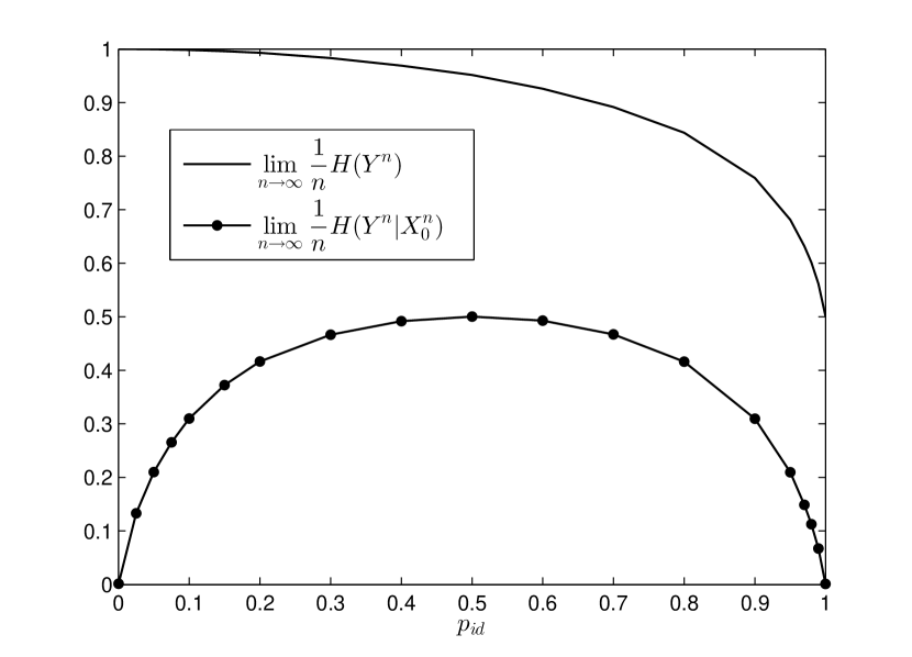
Figure 2: The two terms in Eq. (7) for the i.u.d. input.

$$H\left(Y_{n}\middle|Y_{n-1},X_{n-2},Z_{n-2}\right)={\displaystyle\frac{\alpha p_{d}}{p_{i}+p_{d}}h_{2}(\alpha-\alpha p_{i})}+\frac{p_{i}(1-\alpha p_{d})}{p_{i}+p_{d}}h_{2}\left(A_{1}\right){\displaystyle+\frac{p_{d}(1+\alpha p_{i}-\alpha)}{p_{i}+p_{d}}h_{2}\left(A_{2}\right)}$$ (12)

$$A_{1} ={\displaystyle\frac{1-\alpha-2\alpha p_{d}+\alpha p_{d}^{2}+3\alpha^{2}p_{d}-2\alpha^{2}p_{d}^{2}+\alpha p_{i}p_{d}-\alpha^{2}p_{i}p_{d}}{1-\alpha p_{d}}}$$

$$A_{2} ={\displaystyle\frac{1+2\alpha p_{i}-2\alpha-\alpha p_{i}^{2}-2\alpha^{2}p_{i}+\alpha^{2}+\alpha^{2}p_{i}^{2}-\alpha p_{d}p_{i}+2\alpha^{2}p_{i}p_{d}}{1+\alpha p_{i}-\alpha}}$$

 

$${\displaystyle\lim_{n\to\infty}H\left(Y_{n}\middle|Y^{n-1},X_{0}^{n}\right)}=$$

$${\displaystyle\sum_{k=1}^{\infty}\alpha^{2}\left(1-\alpha\right)^{k-1}\left[{\displaystyle\frac{p_{d}}{p_{i}+p_{d}}h_{2}\left(\frac{p_{d}+p_{i}\left(1-p_{i}-p_{d}\right)^{k}}{p_{i}+p_{d}}\right)}{\displaystyle+\frac{p_{i}}{p_{i}+p_{d}}h_{2}\left(\frac{p_{i}+p_{d}\left(1-p_{i}-p_{d}\right)^{k}}{p_{i}+p_{d}}\right)}\right]}$$ (13)

 

To derive a good lower bound, behaviors of the two terms in Eq. (7) have to be analyzed. Fig. 2 plots the terms for the case of i.u.d. input, using the method in [21], when $p_{i}=p_{d}=p_{id}$. It can be observed that $\lim_{n\to\infty}\frac{1}{n}H\left(Y^{n}\right)$ decreases slowly for low $p_{id}$ (e.g. $p_{id}<0.5$), whereas $\lim_{n\to\infty}\frac{1}{n}H\left(Y^{n}\middle|X_{0}^{n}\right)$ varies drastically. As such, if we are to approximate the capacity for practical values of $p_{id}$, the term $\lim_{n\to\infty}\frac{1}{n}H\left(Y^{n}\middle|X_{0}^{n}\right)$ should be carefully handled, and an estimation of $\lim_{n\to\infty}\frac{1}{n}H\left(Y^{n}\right)$ might be sufficient.

To gain more insights into how the terms could be evaluated, from Eq. (8), notice the following correspondence:

$$\lim_{n\to\infty}\frac{1}{n}H\left(Y^{n}\right) ={\displaystyle\lim_{n\to\infty}H\left(Y_{n}\middle|Y^{n-1}\right)}$$

$$\lim_{n\to\infty}\frac{1}{n}H\left(Y^{n}\middle|X_{0}^{n}\right) =\lim_{n\to\infty}H\left(Y_{n}\middle|Y^{n-1},X_{0}^{n}\right)$$

Since the input is i.u.d., it can be shown that $H\left(Y_{n}\right)=1$ for any $p_{id}$. With the fact that the first term is close to $1$ at low $p_{id}$ whereas the second term differs, one may say, only a few most recent past outputs in $Y^{n-1}$ carry a majority of knowledge about $Y_{n}$ for low $p_{id}$; however, when given $X_{0}^{n}$, farther past outputs are able to resolve more uncertainty about $Y_{n}$ and thus may not be ignored. While this discussion pertains to the i.u.d. input only, the (only) capacity-achieving input is i.u.d. when $p_{id}=0$ (i.e. the channel is noiseless) and so by a continuity argument, at low $p_{id}$, the inputs that achieve the capacity should behave nearly i.u.d.-like and the insights drawn are thus expected to be useful.

Recall that the lower bound established in [8, 9] is the achievable rate with i.u.d. input $C_{iud}$. Now to derive an analytical lower bound that improves on $C_{iud}$, not only do we need to consider a more complex input distribution, but it also cannot be too complicated to analyze. An immediate candidate is its fortiori, a stationary bit-symmetric first-order Markovian input: $P_{\left.X_{n+1}\middle|X_{n}\right.}(1|0)=P_{\left.X_{n+1}\middle|X_{n}\right.}(0|1)=\alpha$ and $P_{X_{0}}(0)=P_{X_{0}}(1)=0.5$. We evaluate each term in Eq. (8) in the following.

IV-A The first term

As discussed, an estimation of this term that retains the first few recent past outputs is sufficient. We lower-bound the term with $Y^{n-2}$ to be discarded:

$$\lim_{n\to\infty}H\left(Y_{n}\middle|Y^{n-1}\right) \geq\lim_{n\to\infty}H\left(Y_{n}\middle|Y^{n-1},X_{0}^{n-2},Z^{n-2}\right)$$

$$\stackrel{{\scriptstyle\left(a\right)}}{{=}}\lim_{n\to\infty}H\left(Y_{n}\middle|Y_{n-1},X_{0}^{n-2},Z^{n-2}\right)$$

$$\stackrel{{\scriptstyle\left(b\right)}}{{=}}\lim_{n\to\infty}H\left(Y_{n}\middle|Y_{n-1},X_{n-2},Z_{n-2}\right)$$

$$\stackrel{{\scriptstyle\left(c\right)}}{{=}}H\left(Y_{n}\middle|Y_{n-1},X_{n-2},Z_{n-2}\right)$$ (11)

where $\left(a\right)$ is because $Y_{i}$ is a function of $Z_{i}$ and $X_{i-1}^{i}$, $\left(b\right)$ is because

$$\left(X_{0}^{n-3},Z^{n-3}\right)\to\left(X_{n-2},Z_{n-2}\right)\to\left(X_{n-2}^{n},Z_{n-1}^{n}\right)\to Y_{n-1}^{n}$$

i.e. they form a Markov chain in that order, and $\left(c\right)$ is due to the following:

$$P_{Y_{n}Y_{n-1}X_{n-2}Z_{n-2}}\left(y_{1},y_{2},x,z\right)$$

$$=\sum_{\begin{subarray}{c}x_{1},x_{2}\\ z_{1},z_{2}\end{subarray}}\left\{\begin{array}[]{c}P_{\left.Y_{n}\middle|X_{n}X_{n-1}Z_{n}\right.}\left(y_{1}\middle|x_{1},x_{2},z_{1}\right)\times\\ P_{\left.Y_{n-1}\middle|X_{n-1}X_{n-2}Z_{n-1}\right.}\left(y_{2}\middle|x_{2},x,z_{2}\right)\times\\ P_{Z_{n-2}^{n}}\left(z_{1},z_{2},z\right)P_{X_{n-2}^{n}}\left(x_{1},x_{2},x\right)\end{array}\right\}$$

$$=\sum_{\begin{subarray}{c}x_{1},x_{2}\\ z_{1},z_{2}\end{subarray}}\left\{\begin{array}[]{c}P_{\left.Y_{n+1}\middle|X_{n+1}X_{n}Z_{n+1}\right.}\left(y_{1}\middle|x_{1},x_{2},z_{1}\right)\times\\ P_{\left.Y_{n}\middle|X_{n}X_{n-1}Z_{n}\right.}\left(y_{2}\middle|x_{2},x,z_{2}\right)\times\\ P_{Z_{n-1}^{n+1}}\left(z_{1},z_{2},z\right)P_{X_{n-1}^{n+1}}\left(x_{1},x_{2},x\right)\end{array}\right\}$$

$$=P_{Y_{n+1}Y_{n}X_{n-1}Z_{n-1}}\left(y_{1},y_{2},x,z\right)$$

for any $\left(y_{1},y_{2},x,z\right)$ and $n\geq 3$, where we make use of the fact that $Y_{n}$ is a time-invariant function of $\left(X_{n},X_{n-1},Z_{n}\right)$ for any $n$, the considered input is stationary, and the capacity is computed w.r.t. stationary $\left\{Z_{n}\right\}_{n=1}^{\infty}$, as mentioned in Section II-A. $H\left(Y_{n}\middle|Y_{n-1},X_{n-2},Z_{n-2}\right)$ is then given by Eq. (12), given that $\left\{Z_{n}\right\}_{n=1}^{\infty}$ attains its stationary distribution as stated.

For a better approximation, repeating the same argument above, we have:

$$\lim_{n\to\infty}H\left(Y_{n}\middle|Y^{n-1}\right) \geq H\left(Y_{n}\middle|Y_{n-\kappa}^{n-1},X_{n-\kappa-1},Z_{n-\kappa-1}\right)$$

for some finite $\kappa\geq 1$. However at relatively low noise, $\kappa=1$ suffices.

IV-B The second term

$$\left[\begin{array}[]{cc}P_{Z_{n}|Z_{n-k}}(0|0)&P_{Z_{n}|Z_{n-k}}(0|1)\\ P_{Z_{n}|Z_{n-k}}(1|0)&P_{Z_{n}|Z_{n-k}}(1|1)\end{array}\right]\;=\;\mathfrak{M}^{k}\;=\;{\displaystyle\frac{1}{p_{i}+p_{d}}\left[\begin{array}[]{cc}p_{d}+p_{i}\left(1-p_{i}-p_{d}\right)^{k}&p_{d}-p_{d}\left(1-p_{i}-p_{d}\right)^{k}\\ p_{i}-p_{i}\left(1-p_{i}-p_{d}\right)^{k}&p_{i}+p_{d}\left(1-p_{i}-p_{d}\right)^{k}\end{array}\right]}$$ (14)

 

$$H\left(Z_{n}\middle|Z_{n-k}\right)={\displaystyle\frac{p_{d}}{p_{i}+p_{d}}h_{2}\left(\frac{p_{d}+p_{i}\left(1-p_{i}-p_{d}\right)^{k}}{p_{i}+p_{d}}\right)+\frac{p_{i}}{p_{i}+p_{d}}h_{2}\left(\frac{p_{i}+p_{d}\left(1-p_{i}-p_{d}\right)^{k}}{p_{i}+p_{d}}\right)}$$ (15)

 

$$C_{Mkv}^{lb}=\max_{\alpha\in\left[0,1\right]}\left[H\left(Y_{n}\middle|Y_{n-1},X_{n-2},Z_{n-2}\right)-\lim_{n\to\infty}H\left(Y_{n}\middle|Y^{n-1},X_{0}^{n}\right)\right]_{{\displaystyle X_{0}^{\infty}\sim\mbox{Markov}\left(\alpha\right)}}$$ (16)

 

Lemma 15.

$\lim_{n\to\infty}H\left(Y_{n}\middle|Y^{n-1},X_{0}^{n}\right)$ is given by Eq. (13), in which $\alpha=P\left(X_{i}\neq X_{i-1}\right)$, for any stationary input.

Proof:

$\alpha$ exists thanks to stationarity of the input. We make a few observations:

(Ob.1) Given $X_{i}\neq X_{i-1}$, knowledge (or respectively, uncertainty) about $Y_{i}$ is equivalent to knowledge (or respectively, uncertainty) about $Z_{i}$.

(Ob.2) Given $X_{i}=X_{i-1}$, uncertainty about $Y_{i}$ is completely resolved, and knowledge of $Y_{i}$ provides no information about $Z_{i}$.

(Ob.3) Without knowing $Y_{i}$, knowledge of $X_{i}$ also provides no information about $Z_{i}$, since the input $X_{0}^{n}$ and the channel state $Z^{n}$ are independent.

(Ob.4) As for resolving uncertainty about $Z_{i}$, knowledge of $Y^{i-1}$ and $X_{0}^{i-1}$ is only as good as to provide (partial) knowledge of $Z^{i-1}$. Furthermore, since $Z^{n}$ is a first-order Markov process, in the resolution of uncertainty about $Z_{i}$, for $q\leq k\leq i-1$, knowing $Z_{q}^{k}$ (without knowledge of $Z_{k+1}^{i-1}$, if $k<i-1$) is the same as knowing $Z_{k}$.

We then have:

$$H\left(Y_{n}\middle|Y^{n-1},X_{0}^{n}\right)$$

$$=H\left(Y_{n}\middle|Y^{n-1},X_{0}^{n},X_{n}=X_{n-1}\right)P\left(X_{n}=X_{n-1}\right)$$

$$\quad+H\left(Y_{n}\middle|Y^{n-1},X_{0}^{n},X_{n}\neq X_{n-1}\right)P\left(X_{n}\neq X_{n-1}\right)$$

$$=\alpha H\left(Z_{n}\middle|Y^{n-1},X_{0}^{n},X_{n}\neq X_{n-1}\right)$$

$$=\alpha H\left(Z_{n}\middle|Y^{n-1},X_{0}^{n-1}\right)$$

$$H\left(Z_{n}\middle|Y^{n-1},X_{0}^{n-1}\right)$$

$$=\alpha H\left(Z_{n}\middle|Y^{n-1},X_{0}^{n-1},X_{n-1}\neq X_{n-2}\right)$$

$$\quad+\left(1-\alpha\right)H\left(Z_{n}\middle|Y^{n-1},X_{0}^{n-1},X_{n-1}=X_{n-2}\right)$$

$$=\alpha H\left(Z_{n}\middle|Z_{n-1}\right)+\left(1-\alpha\right)H\left(Z_{n}\middle|Y^{n-2},X_{0}^{n-2}\right)$$

Similarly:

$$H\left(Z_{n}\middle|Y^{n-2},X_{0}^{n-2}\right)$$

$$=\alpha H\left(Z_{n}\middle|Z_{n-2}\right)+\left(1-\alpha\right)H\left(Z_{n}\middle|Y^{n-3},X_{0}^{n-3}\right)$$

$$\ldots$$

$$H\left(Z_{n}\middle|Y_{1},X_{0}^{1}\right)=\alpha H\left(Z_{n}\middle|Z_{1}\right)+\left(1-\alpha\right)H\left(Z_{n}\right)$$

We are then left with evaluating $H\left(Z_{n}\middle|Z_{n-k}\right)$ for $k=1,\ldots,n-1$. Consider

$$\mathfrak{M} =\left[\begin{array}[]{cc}P_{Z_{n}|Z_{n-1}}(0|0)&P_{Z_{n}|Z_{n-1}}(0|1)\\ P_{Z_{n}|Z_{n-1}}(1|0)&P_{Z_{n}|Z_{n-1}}(1|1)\end{array}\right]$$

$$=\left[\begin{array}[]{cc}1-p_{i}&p_{d}\\ p_{i}&1-p_{d}\end{array}\right]$$

We then obtain Eq. (14). Subsequently $H\left(Z_{n}\middle|Z_{n-k}\right)$ is given by Eq. (15). Putting everything together, we obtain the lemma. ∎

When the input is the aforementioned first-order Markovian process, $\alpha$ given in Eq. (13) is also $P_{\left.X_{n+1}\middle|X_{n}\right.}(1|0)=P_{\left.X_{n+1}\middle|X_{n}\right.}(0|1)$.

Now combining Eq. (12) and (13), the new lower bound $C_{Mkv}^{lb}$ is then given by Eq. (16). The maximization is reduced to a univariate one (i.e. maximization in $\alpha$), which can be computed efficiently. The results are given in Fig. 3 and 4. It can be observed that $C_{Mkv}^{lb}$ has improved over $C_{iud}$, given in [8], for most values of $p_{id}$. We also note, the fact that $C_{iud}^{lb}$ (which is $C_{Mkv}^{lb}$ with unoptimized $\alpha=0.5$) is close to $C_{iud}$ shows that the estimation in Eq. (11) is not a bad one as previously expected.

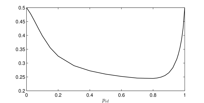
Figure 3: Optimized $\alpha$ for $C_{Mkv}^{lb}$.

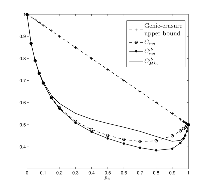
Figure 4: New lower bound $C_{Mkv}^{lb}$. Here $C_{iud}^{lb}$ is $C_{Mkv}^{lb}$ with unoptimized $\alpha=0.5$ (i.e. i.u.d. input) for all $p_{id}$.

The bounding technique here relies on the exact establishment of the second entropy term. While Lemma 15 is heavily channel-dependent, we make a short note on how the strategy could be extended to calculate the entropy term when $Z_{i}$ has a larger alphabet. For example, consider ${\cal Z}=\left\{0,1,2\right\}$, and the term is then $\lim_{n\to\infty}H\left(Y_{n}\middle|Y^{n-1},X_{-1}^{n}\right)$. Consider the following $4$ variables:

$$\alpha_{1} =P\left(X_{n}=X_{n-1}=X_{n-2}\right)$$

$$\alpha_{2} =P\left(X_{n}=X_{n-1}\neq X_{n-2}\right)$$

$$\alpha_{3} =P\left(X_{n}\neq X_{n-1}=X_{n-2}\right)$$

$$\alpha_{4} =P\left(X_{n-1}\neq X_{n}=X_{n-2}\right)$$

$\left\{\alpha_{1},\alpha_{2},\alpha_{3},\alpha_{4}\right\}$ plays the role as $\alpha$ in Lemma 15 and can be reduced in size via the stationarity condition and also the fact $\alpha_{1}+\alpha_{2}+\alpha_{3}+\alpha_{4}=1$. The key to the extension is to realize that similar to (Ob.1) and (Ob.2), given an event that corresponds to one among $\alpha_{1},\alpha_{2},\alpha_{3},\alpha_{4}$, the uncertainty of $Y_{i}$ could be partially reduced to that of $Z_{i}$, and knowledge of $Y_{i}$ is partially equivalent to that of $Z_{i}$. For example,

$$H\left(Y_{n}\middle|Y^{n-1},X_{-1}^{n},X_{n}\neq X_{n-1}=X_{n-2}\right)$$

$$=H\left(Z_{n}^{\left(12\right)}\middle|Y^{n-1},X_{-1}^{n},X_{n}\neq X_{n-1}=X_{n-2}\right)$$

$$=H\left(Z_{n}^{\left(12\right)}\middle|Y^{n-1},X_{-1}^{n-1}\right)$$

$$H\left(Z_{n}^{\left(12\right)}\middle|Y^{n-1},X_{-1}^{n-1},X_{n-2}\neq X_{n-1}=X_{n-3}\right)$$

$$=H\left(Z_{n}^{\left(12\right)}\middle|Z_{n-1}^{\left(02\right)},Y^{n-1},X_{-1}^{n-1},X_{n-2}\neq X_{n-1}=X_{n-3}\right)$$

$$=H\left(Z_{n}^{\left(12\right)}\middle|Z_{n-1}^{\left(02\right)},Y^{n-2},X_{-1}^{n-2}\right)$$

where $Z_{n}^{\left(jk\right)}=\mathbb{I}\left(Z_{n}\in\left\{j,k\right\}\right)$. Here $\mathbb{I}\left(A\right)$ is $1$ if $A$ is true and $0$ otherwise.

V DID Channel Capacity Upper Bound

In this section, we formulate a new series of computable upper bounds with a parameter ${\cal L}$. The upper bounds improve as ${\cal L}$ increases, and match up with the developed lower bound at low noise levels. We also discuss the crucial role of the input stationarity condition in the new upper bounds, without which the bounds could be trivialized.

V-A Formulation and Computation

An upper bound is usually difficult to establish analytically, since it involves maximization over all input distributions, unlike lower bounds. We shall rely on computational methods. To do so, we assume stationary inputs and bound each term in Eq. (8) as follows. Let $\mathcal{L}\geq 1$ be a given finite parameter to control the accuracy of the to-be-formulated upper bound. For any $n\geq 1$, we have:

$$H\left(Y_{n+{\cal L}}\middle|Y^{n+{\cal L}-1}\right)\leq H\left(Y_{n+{\cal L}}\middle|Y_{n+1}^{n+{\cal L}-1}\right)$$

Note that the right-hand side is independent of $n$ by stationarity. As such,

$$\lim_{n\to\infty}H\left(Y_{n}\middle|Y^{n-1}\right)\leq H\left(Y_{n+{\cal L}}\middle|Y_{n+1}^{n+{\cal L}-1}\right)$$ (17)

Next, notice that in the resolution of uncertainty in $Y_{i}$, given $X_{i-1}^{i}$, other random variables can help at best by providing information about $Z_{i}$. Together with observation (Ob.4) made earlier, we have the Markov chain

$$\left(Y^{n},X_{0}^{n-1}\right)\to\left(Y_{n+1}^{n+{\cal L}-1},X_{n}^{n+{\cal L}},Z_{n}\right)\to Y_{n+{\cal L}}$$

Therefore:

$$H\left(Y_{n+{\cal L}}\middle|Y^{n+{\cal L}-1},X_{0}^{n+{\cal L}}\right) \geq H\left(Y_{n+{\cal L}}\middle|Y^{n+{\cal L}-1},X_{0}^{n+{\cal L}},Z_{n}\right)$$

$$=H\left(Y_{n+{\cal L}}\middle|Y_{n+1}^{n+{\cal L}-1},X_{n}^{n+{\cal L}},Z_{n}\right)$$

whose right-hand side is independent of $n$ for the same reason that leads to Eq. (11). Then:

$$\lim_{n\to\infty}H\left(Y_{n}\middle|Y^{n-1},X_{0}^{n}\right)\geq H\left(Y_{n+{\cal L}}\middle|Y_{n+1}^{n+{\cal L}-1},X_{n}^{n+{\cal L}},Z_{n}\right)$$ (18)

By Eq. (17) and (18), letting

$$C_{\mathcal{L}}^{ub}\left(P_{X_{n}^{n+{\cal L}}}\right)$$

$$=H\left(Y_{n+{\cal L}}\middle|Y_{n+1}^{n+{\cal L}-1}\right)-H\left(Y_{n+{\cal L}}\middle|Y_{n+1}^{n+{\cal L}-1},X_{n}^{n+{\cal L}},Z_{n}\right)$$

we have

$$C\leq C_{\mathcal{L}}^{ub}\equiv\sup_{\begin{subarray}{c}\text{Stationary, bit-symmetric}\\ P_{X_{n}^{n+{\cal L}}}\end{subarray}}C_{\mathcal{L}}^{ub}\left(P_{X_{n}^{n+{\cal L}}}\right)$$

Then $C_{\mathcal{L}}^{ub}$ gives a capacity upper bound, controlled by $\mathcal{L}$.

To compute this bound, we turn to the following lemma, which is a straightforward exercise.

Lemma 16.

Given vectors $w_{i},q_{i}\in\mathbb{R}^{n}$ and variable $u\in\mathbb{R}^{n}$, define a function $f(u)=-\sum_{i}w_{i}^{\top}u\log\left(w_{i}^{\top}u\left/q_{i}^{\top}u\right)\right.$ where $\mbox{dom}(f)=\{u:\;w_{i}^{\top}u\geq 0\;\forall i\}$. Then $f$ is a concave function.

It is easy to see that $H\left(Y_{n+{\cal L}}\middle|Y_{n+1}^{n+{\cal L}-1},X_{n}^{n+{\cal L}},Z_{n}\right)$ is affine in $P_{X_{n}^{n+{\cal L}}}$, and $H\left(Y_{n+{\cal L}}\middle|Y_{n+1}^{n+{\cal L}-1}\right)$ takes the form of function $f$ in the above lemma with $P_{X_{n}^{n+{\cal L}}}$ being the variable $u$. Then $C_{\mathcal{L}}^{ub}\left(P_{X_{n}^{n+{\cal L}}}\right)$ is a concave function. We note the following:

• $P_{X_{n}^{n+{\cal L}}}$ being a valid probability measure means $\sum_{\mathbf{x}}P_{X_{n}^{n+{\cal L}}}\left(\mathbf{x}\right)=1$ (unity-sum condition) and $P_{X_{n}^{n+{\cal L}}}\left(\mathbf{x}\right)\geq 0$ (non-negativity condition) $\forall\mathbf{x}\in\mbox{GF}(2)^{\mathcal{L}+1}$.

• The stationarity condition is linear and hence can be converted into the form $Sp_{X}=0$, where $p_{X}=\left[\begin{array}[]{ccc}...&P_{X_{n}^{n+{\cal L}}}\left(\mathbf{x}\right)&...\end{array}\right]^{\top}$ and $S$ is a matrix. For example, when $\mathcal{L}=1$, we have:

  $$p_{X}=\left[\begin{array}[]{c}P_{X_{n}^{n+1}}\left(0,0\right)\\ P_{X_{n}^{n+1}}\left(0,1\right)\\ P_{X_{n}^{n+1}}\left(1,0\right)\\ P_{X_{n}^{n+1}}\left(1,1\right)\end{array}\right]\quad S=\left[\begin{array}[]{clcc}0&1&-1&0\end{array}\right]$$

  which represents $P_{X_{n}}\left(0\right)=P_{X_{n+1}}\left(0\right)$ and $P_{X_{n}}\left(1\right)=P_{X_{n+1}}\left(1\right)$. In general, $S$ can be constructed efficiently by computations. The following lemma indicates that the number of rows in $S$ is at most $2^{\mathcal{L}}-1$, i.e. it grows linearly with the size of $p_{X}$ and so using the stationarity condition in computations is not too costly.

Lemma 17.

For any finite $n$ and random vector $V^{n}\in\text{GF}(2)^{n}$ with probability distribution $P$, it is stationary if and only if, for any $\mathbf{v}\in\text{GF}(2)^{n-1}$,

$$P\left(V_{1}^{n-1}=\mathbf{v}\right)=P\left(V_{2}^{n}=\mathbf{v}\right)$$ (19)

In fact, if Eq. (19) is satisfied for any $2^{n-1}-1$ vectors $\mathbf{v}$ from $\text{GF}(2)^{n-1}$, it is also satisfied for the other $\mathbf{v}\in\text{GF}(2)^{n-1}$.

Proof:

Let us consider the first claim. The forward is immediate. We prove the converse. Since $V^{n}$ is defined over $\mbox{GF}(2)$, any event on it implies that a subset of entries in $\{V_{i}:\;i=1,...,n\}$ takes up a specific value. Consider an arbitrary event $E=\left\{V_{i}=a_{i},\;i\in N_{E}\right\}$ for any $N_{E}\subseteq\left\{1,...,n-1\right\}$. Then if for any such event, $P(E)=P(T^{-s}E)$ for $s=1,...,n-\max N_{E}$, $P$ is stationary. Assume that for any $\mathbf{v}\in\mbox{GF}(2)^{n-1}$, $P\left(V_{1}^{n-1}=\mathbf{v}\right)=P\left(V_{2}^{n}=\mathbf{v}\right)$. We have:

$$P(T^{-s}E) =\sum_{\begin{subarray}{c}v_{i+s-1}=a_{i},\;i\in N_{E}\\ v_{j+s-1}\in\text{GF}(2),\;j\notin N_{E}\end{subarray}}P\left(V_{2}^{n}=\mathbf{v}\right)$$

$$=\sum_{\begin{subarray}{c}v_{i+s-1}=a_{i},\;i\in N_{E}\\ v_{j+s-1}\in\text{GF}(2),\;j\notin N_{E}\end{subarray}}P\left(V_{1}^{n-1}=\mathbf{v}\right)$$

$$=\sum_{\begin{subarray}{c}v_{i+s-2}=a_{i},\;i\in N_{E}\\ v_{j+s-2}\in\text{GF}(2),\;j\notin N_{E}\end{subarray}}P\left(V_{2}^{n}=\mathbf{v}\right)$$

$$=\sum_{\begin{subarray}{c}v_{i+s-2}=a_{i},\;i\in N_{E}\\ v_{j+s-2}\in\text{GF}(2),\;j\notin N_{E}\end{subarray}}P\left(V_{1}^{n-1}=\mathbf{v}\right)$$

$$\ldots$$

$$=\sum_{\begin{subarray}{c}v_{i}=a_{i},\;i\in N_{E}\\ v_{j}\in\text{GF}(2),\;j\notin N_{E}\end{subarray}}P\left(V_{2}^{n}=\mathbf{v}\right)$$

$$=\sum_{\begin{subarray}{c}v_{i}=a_{i},\;i\in N_{E}\\ v_{j}\in\text{GF}(2),\;j\notin N_{E}\end{subarray}}P\left(V_{1}^{n-1}=\mathbf{v}\right)$$

$$=P(E)$$

The first claim is hence proven.

To see the second claim, notice Eq. (19) can be written as

$$P_{V^{n}}\left(\left[\mathbf{v},0\right]\right)+P_{V^{n}}\left(\left[\mathbf{v},1\right]\right)=P_{V^{n}}\left(\left[0,\mathbf{v}\right]\right)+P_{V^{n}}\left(\left[1,\mathbf{v}\right]\right)$$

Summing both sides over all $\mathbf{v}\in\mbox{GF}(2)^{n-1}$, we then obtain a trivial equation, which implies one redundant equation in the system. ∎

• The condition of bit-symmetry is also equivalent to a set of linear equations $P_{X_{n}^{n+{\cal L}}}\left(\mathbf{x}\right)=P_{X_{n}^{n+{\cal L}}}\left(\neg\mathbf{x}\right)$ $\forall\mathbf{x}\in\mbox{GF}(2)^{\mathcal{L}+1}$. In fact, this condition is not even needed: one can easily establish a result for $C_{\mathcal{L}}^{ub}$ similar to Proposition 4 using the same technique, i.e.

  $$\sup_{\begin{subarray}{c}\text{Stationary}\\ P_{X_{n}^{n+{\cal L}}}\end{subarray}}C_{\mathcal{L}}^{ub}\left(P_{X_{n}^{n+{\cal L}}}\right)=\sup_{\begin{subarray}{c}\text{Bit-symmetric,}\\ \text{stationary }P_{X_{n}^{n+{\cal L}}}\end{subarray}}C_{\mathcal{L}}^{ub}\left(P_{X_{n}^{n+{\cal L}}}\right)$$

With those points made above, we conclude that finding $C_{\mathcal{L}}^{ub}$ is a convex optimization problem, which can be efficiently solved using various computational methods [22]. The results are shown in Fig. 5 for $\mathcal{L}=2,3,...,7$. It can be observed that the series of upper bounds improves over the genie-erasure upper bound, given in [8], for most values of $p_{id}$ and approaches closely to the new lower bound $C_{Mkv}^{lb}$ at low $p_{id}$.

The complexity of the program to find $C_{\mathcal{L}}^{ub}$ scales rapidly with ${\cal L}$: it increases polynomially with the number of variables $2^{{\cal L}+1}$ and the number of equality constraints $2^{{\cal L}}$ (including the stationarity condition and the unity-sum condition, excluding the bit-symmetry condition). Nevertheless Fig. 5 suggests that the upper bounds converge quickly with ${\cal L}$, so small ${\cal L}$ is sufficient to produce decent results.

In Fig. 6, we also compare our new bounds to those in [9], which were derived for the case $p_{d}=1$. Improvements are observed.

As a note, Lemma 15 should not be used in place of Eq. (18); otherwise the maximization problem would be a non-convex one.

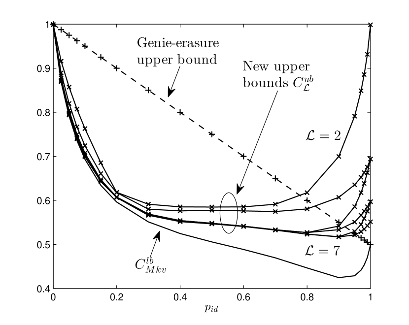
Figure 5: New upper bounds $C_{\mathcal{L}}^{ub}$ for $\mathcal{L}=2,3,...,7$. The higher curve corresponds to the lower $\mathcal{L}$.

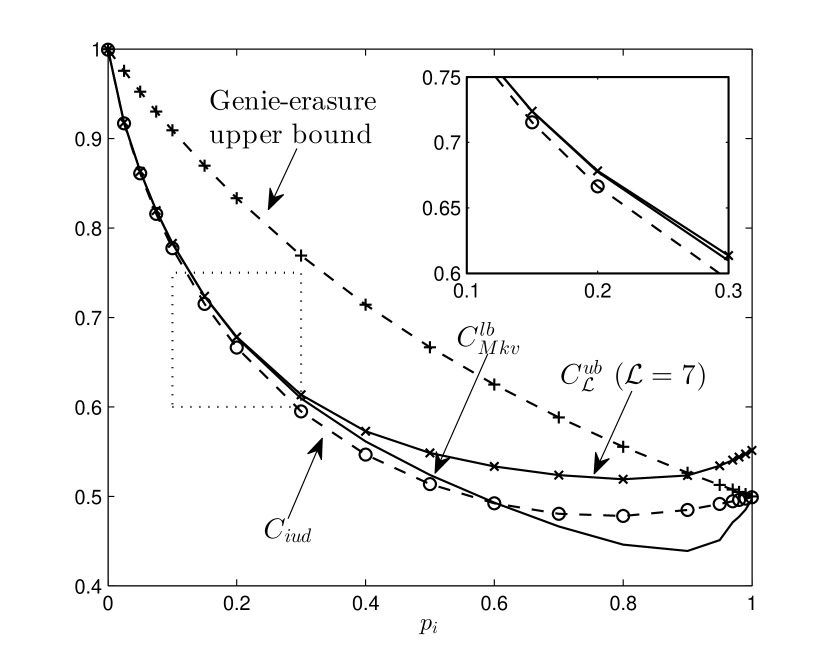
Figure 6: New bounds for the case $p_{d}=1$ in comparison with bounds derived in [9] (dashed curves).

V-B Tightness of the New Upper Bounds

It is easy to see that the bound is improved monotonically with increasing $\mathcal{L}$. Indeed,

$$H\left(Y_{n+{\cal L}+1}\middle|Y_{n+1}^{n+{\cal L}}\right) =H\left(Y_{n+{\cal L}}\middle|Y_{n}^{n+{\cal L}-1}\right)$$

$$\leq H\left(Y_{n+{\cal L}}\middle|Y_{n+1}^{n+{\cal L}-1}\right)$$

where the first equation is because of the channel output's stationarity, given that the channel and the input are stationary. We also have:

$$H\left(Y_{n+{\cal L}+1}\middle|Y_{n+1}^{n+{\cal L}},X_{n}^{n+{\cal L}+1},Z_{n}\right)$$

$$=H\left(Y_{n+{\cal L}}\middle|Y_{n}^{n+{\cal L}-1},X_{n-1}^{n+{\cal L}},Z_{n-1}\right)$$

$$\geq H\left(Y_{n+{\cal L}}\middle|Y_{n}^{n+{\cal L}-1},X_{n-1}^{n+{\cal L}},Z_{n-1},Z_{n}\right)$$

$$=H\left(Y_{n+{\cal L}}\middle|Y_{n+1}^{n+{\cal L}-1},X_{n}^{n+{\cal L}},Z_{n}\right)$$

where the first and last equalities are by arguing in a similar manner to the derivation of Eq. (11) and (18) respectively. These show that

$$C_{\mathcal{L}+1}^{ub}\left(P_{X_{n}^{n+{\cal L}+1}}\right)\leq C_{\mathcal{L}}^{ub}\left(P_{X_{n}^{n+{\cal L}}}\right)$$

where $P_{X_{n}^{n+{\cal L}}}$ is a marginal distribution of $P_{X_{n}^{n+{\cal L}+1}}$. Taking the supremum, we obtain $C\leq C_{\mathcal{L}+1}^{ub}\leq C_{\mathcal{L}}^{ub}$.

We next discuss the gap between $C$ and $C_{\infty}^{ub}$. Here $C_{\infty}^{ub}$ exists since $C_{{\cal L}}^{ub}$ decreases with increasing ${\cal L}$ and is bounded from below. We first connect $C$ and $C_{\mathcal{L}}^{ub}\left(P_{X_{n}^{n+{\cal L}}}\right)$ by establishing the following:

$$C_{\mathcal{L}}^{ub}\left(P_{X_{n}^{n+{\cal L}}}\right)\xrightarrow{\mathcal{L}\to\infty}$$

$$\left[\lim_{n\to\infty}H\left(Y_{n}\middle|Y^{n-1}\right)-\lim_{n\to\infty}H\left(Y_{n}\middle|Y^{n-1},X_{0}^{n}\right)\right]_{X_{0}^{\infty}\sim P_{X_{0}^{\infty}}}$$

where the right-hand side is evaluated w.r.t. a stationary input distribution $P_{X_{0}^{\infty}}$ such that for every ${\cal L}$, $P_{X_{n}^{n+{\cal L}}}$ is a marginal distribution of $P_{X_{0}^{\infty}}$. Let $g\left(P_{X_{0}^{\infty}}\right)$ denote the right-hand side. Since $P_{X_{0}^{\infty}}$ is stationary, all $\left({\cal L}+1\right)$-dimensional marginals of $P_{X_{0}^{\infty}}$ are the same. We can then regard $C_{\mathcal{L}}^{ub}\left(\cdot\right)$ as a function of $P_{X_{0}^{\infty}}$. With an abuse of notation, we write $C_{\mathcal{L}}^{ub}\left(P_{X_{0}^{\infty}}\right)$ to mean $C_{\mathcal{L}}^{ub}\left(P_{X_{n}^{n+{\cal L}}}\right)$. It is easy to see that

$$C_{\mathcal{L}}^{ub}\left(P_{X_{0}^{\infty}}\right)$$

$$=H\left(Y_{n+{\cal L}}\middle|Y_{n+1}^{n+{\cal L}-1}\right)+H\left(Z_{n}\middle|Y_{n+1}^{n+{\cal L}-1},X_{n}^{n+{\cal L}}\right)$$

$$\quad-H\left(Y_{n+{\cal L}}\middle|Y_{n+1}^{n+{\cal L}-1},X_{n}^{n+{\cal L}}\right)-H\left(Z_{n}\middle|Y_{n+1}^{n+{\cal L}},X_{n}^{n+{\cal L}}\right)$$

Notice that

$$H\left(Z_{n}\middle|Y_{n+1}^{n+{\cal L}-1},X_{n}^{n+{\cal L}}\right) \leq H\left(Z_{n}\middle|Y_{n+1}^{n+{\cal L}-1},X_{n}^{n+{\cal L}-1}\right)$$

$$H\left(Z_{n}\middle|Y_{n+1}^{n+{\cal L}-1},X_{n}^{n+{\cal L}}\right) \geq H\left(Z_{n}\middle|Y_{n+1}^{n+{\cal L}},X_{n}^{n+{\cal L}}\right)$$

whereas

$$\lim_{\mathcal{L\to\infty}}H\left(Z_{n}\middle|Y_{n+1}^{n+{\cal L}-1},X_{n}^{n+{\cal L}-1}\right)$$

$$\quad=\lim_{\mathcal{L\to\infty}}H\left(Z_{n}\middle|Y_{n+1}^{n+{\cal L}},X_{n}^{n+{\cal L}}\right)$$

Furthermore, thanks to stationarity of the channel output and the joint input-output distribution,

$$\lim_{\mathcal{L\to\infty}}H\left(Y_{n+{\cal L}}\middle|Y_{n+1}^{n+{\cal L}-1}\right) ={\displaystyle\lim_{n\to\infty}H\left(Y_{n}\left|Y^{n-1}\right)\right.}$$

$$\lim_{\mathcal{L\to\infty}}H\left(Y_{n+{\cal L}}\middle|Y_{n+1}^{n+{\cal L}-1},X_{n}^{n+{\cal L}}\right) =\lim_{n\to\infty}H\left(Y_{n}\middle|Y^{n-1},X_{0}^{n}\right)$$

Therefore, $C_{\mathcal{L}}^{ub}\left(P_{X_{0}^{\infty}}\right)\to g\left(P_{X_{0}^{\infty}}\right)$ as ${\cal L}\to\infty$, for any stationary distribution $P_{X_{0}^{\infty}}$. Now notice that

$$C=\sup_{\text{Stationary }P_{X_{0}^{\infty}}}g\left(P_{X_{0}^{\infty}}\right)=\sup_{\text{Stationary }P_{X_{0}^{\infty}}}\lim_{{\cal L}\to\infty}C_{\mathcal{L}}^{ub}\left(P_{X_{0}^{\infty}}\right)$$

whereas

$$C_{\infty}^{ub}=\lim_{{\cal L}\to\infty}\sup_{\text{Stationary }P_{X_{0}^{\infty}}}C_{\mathcal{L}}^{ub}\left(P_{X_{0}^{\infty}}\right)$$

The gap hence lies in the order of the limit and the supremum. This is a consequence of computational feasibility: restriction to finite-dimensional distributions $P_{X_{n}^{n+{\cal L}}}$ is required for computations, whereas $C$ is inherently a quantity with infinite block lengths. We conjecture that no other upper-bounding methods that directly modify the entropy terms in Eq. (8) (or the mutual information term in Eq. (6)) are better than the presented one. If the discussed gap is non-trivial and one seeks a better upper bound, a different formulation of the capacity might be called for.

In fact, in the Shannon-theoretic framework, it shall be proven that the gap is trivial, i.e. $C_{\infty}^{ub}=C$! We have:

$${\cal L}C_{{\cal L}}^{ub}\left(P_{X_{0}^{\infty}}\right)\stackrel{{\scriptstyle\left(a\right)}}{{\leq}}\sum_{j=1}^{{\cal L}}C_{j}^{ub}\left(P_{X_{0}^{\infty}}\right)$$

$$=\sum_{j=1}^{{\cal L}}H\left(Y_{n+j}\middle|Y_{n+1}^{n+j-1}\right)-H\left(Y_{n+j}\middle|Y_{n+1}^{n+j-1},X_{n}^{n+j},Z_{n}\right)$$

$$\leq\sum_{j=1}^{{\cal L}}H\left(Y_{n+j}\middle|Y_{n+1}^{n+j-1}\right)-H\left(Y_{n+j}\middle|Y_{n+1}^{n+j-1},X_{n}^{n+{\cal L}},Z_{n}\right)$$

$$=H\left(Y_{n+1}^{n+{\cal L}}\right)-H\left(Y_{n+1}^{n+{\cal L}}\middle|X_{n}^{n+{\cal L}},Z_{n}\right)$$

$$=I\left(X_{n}^{n+{\cal L}};Y_{n+1}^{n+{\cal L}}\right)+I\left(Z_{n};Y_{n+1}^{n+{\cal L}}\middle|X_{n}^{n+{\cal L}}\right)$$

and therefore

$$C_{\infty}^{ub} \leq\lim_{{\cal L}\to\infty}\frac{1}{{\cal L}}\sup_{\text{Stationary }P_{X_{0}^{\infty}}}I\left(X_{n}^{n+{\cal L}};Y_{n+1}^{n+{\cal L}}\right)$$

$$\quad+\lim_{{\cal L}\to\infty}\frac{1}{{\cal L}}\sup_{\text{Stationary }P_{X_{0}^{\infty}}}I\left(Z_{n};Y_{n+1}^{n+{\cal L}}\middle|X_{n}^{n+{\cal L}}\right)$$

$$\stackrel{{\scriptstyle\left(b\right)}}{{=}}\lim_{{\cal L}\to\infty}\frac{1}{{\cal L}}\sup_{\text{Stationary }P_{X_{0}^{\infty}}}I\left(X_{n}^{n+{\cal L}};Y_{n+1}^{n+{\cal L}}\right)$$

$$\stackrel{{\scriptstyle\left(c\right)}}{{=}}\lim_{n\to\infty}\frac{1}{n}\sup_{\text{Stationary }P_{X_{0}^{\infty}}}I\left(X_{0}^{n};Y_{1}^{n}\right)$$

$$\leq\lim_{n\to\infty}\frac{1}{n}\sup_{X_{0}^{n}}I\left(X_{0}^{n};Y_{1}^{n}\right)$$

$$\stackrel{{\scriptstyle\left(d\right)}}{{=}}C$$

Here $\left(a\right)$ is because $C_{j+1}^{ub}\left(P_{X_{0}^{\infty}}\right)\leq C_{j}^{ub}\left(P_{X_{0}^{\infty}}\right)$ as proven above, $\left(b\right)$ is because

$$0\leq\frac{1}{{\cal L}}I\left(Z_{n};Y_{n+1}^{n+{\cal L}}\middle|X_{n}^{n+{\cal L}}\right)\leq\frac{1}{{\cal L}}\log\left|{\cal Z}\right|=\frac{1}{{\cal L}}\to 0$$

$\left(c\right)$ is because of stationarity, and $\left(d\right)$ is Eq. (10), stemming from the fact the DID channel is an indecomposable FSC in the Shannon-theoretic framework. Finally, since $C\leq C_{\infty}^{ub}$, we have $C_{\infty}^{ub}=C$.

Aside from increasing ${\cal L}$, one may expect to obtain a better upper bound by adding more constraints on the input search space. Note, however, not all constraints would help. One example is bit-symmetry as pointed out earlier. An opposite example is the stationarity condition, which is discussed next.

V-C Importance of the Stationary Condition

We shed light on why the stationarity condition is crucial to developing meaningful upper bounds. In particular, without this condition, they could be trivialized, i.e. equal to $1$. To this end, let us consider the following quantity:

$$U_{\mathcal{L}}\equiv\sup_{P_{X_{n}^{n+{\cal L}}}}C_{\mathcal{L}}^{ub}\left(P_{X_{n}^{n+{\cal L}}}\right)$$

which is essentially $C_{\mathcal{L}}^{ub}$ without input stationarity. Notice that when the input is not stationary, $C_{\mathcal{L}}^{ub}\left(P_{X_{n}^{n+{\cal L}}}\right)$ is implicitly a function of $n$, denoted by $\gamma\left(n\right)$ to emphasize this dependency. In a similar manner to the derivation of Eq. (11), it is easy to see that if $P_{X_{n}^{n+{\cal L}}}=P^{*}$ yields the supremum of $\gamma\left(n\right)$ then $P_{X_{n+1}^{n+{\cal L}+1}}=P^{*}$ yields the supremum of $\gamma\left(n+1\right)$. As such, the supremum in $U_{\mathcal{L}}$ is independent of $n$, i.e. $U_{\mathcal{L}}$ is not a function of $n$.

First, we need to justify that $U_{\mathcal{L}}$ is a valid upper bound on $C$. This is indeed the case since $U_{\mathcal{L}}\geq C_{\mathcal{L}}^{ub}\geq C$. Alternatively this can be shown without resorting to $C_{\mathcal{L}}^{ub}$ as follows. We modify Eq. (17) and (18):

$$\lim_{n\to\infty}H\left(Y_{n}\middle|Y^{n-1}\right)\leq\liminf_{n\to\infty}H\left(Y_{n+{\cal L}}\middle|Y_{n+1}^{n+{\cal L}-1}\right)$$

$$\lim_{n\to\infty}H\left(Y_{n}\middle|Y^{n-1},X_{0}^{n}\right)$$

$$\quad\geq\limsup_{n\to\infty}H\left(Y_{n+{\cal L}}\middle|Y_{n+1}^{n+{\cal L}-1},X_{n}^{n+{\cal L}},Z_{n}\right)$$

which are valid without the restriction to stationary inputs. Then:

$$C \leq\sup\left\{\begin{array}[]{c}{\displaystyle\liminf_{n\to\infty}H\left(Y_{n+{\cal L}}\middle|Y_{n+1}^{n+{\cal L}-1}\right)-}\\ {\displaystyle\limsup_{n\to\infty}H\left(Y_{n+{\cal L}}\middle|Y_{n+1}^{n+{\cal L}-1},X_{n}^{n+{\cal L}},Z_{n}\right)}\end{array}\right\}$$

$$\leq\sup\liminf_{n\to\infty}C_{\mathcal{L}}^{ub}\left(P_{X_{n}^{n+{\cal L}}}\right)$$

$$\leq\liminf_{n\to\infty}\sup C_{\mathcal{L}}^{ub}\left(P_{X_{n}^{n+{\cal L}}}\right)\stackrel{{\scriptstyle\left(a\right)}}{{=}}U_{\mathcal{L}}$$

where the suprema are over all valid inputs, and $\left(a\right)$ is because $U_{{\cal L}}$ is independent of $n$.

We now show that $U_{{\cal L}}=1$ in the case $p_{i}=p_{d}$ for any $\mathcal{L}\geq 2$. Consider a specific input distribution $P_{X_{n}^{n+{\cal L}}}^{*}$ such that

$$P\left(X_{n}^{n+{\cal L}}=...1010100\right)=P\left(X_{n}^{n+{\cal L}}=...0101011\right)=0.5$$

i.e. only two input strings with identical first two bits and alternating bits thereafter are assigned probability $0.5$. It is easy to see that $P_{X_{n}^{n+{\cal L}}}^{*}$ is not stationary. With probability $1$, we have $X_{n+{\cal L}}=X_{n+{\cal L}-1}$, which completely resolves uncertainty in $Y_{n+{\cal L}}$, and so $H\left(Y_{n+{\cal L}}\middle|Y_{n+1}^{n+{\cal L}-1},X_{n}^{n+{\cal L}},Z_{n}\right)=0$. For any $\mathbf{y}\in\mbox{GF}(2)^{\mathcal{L}-1}$,

$$P\left(Y_{n+{\cal L}}=0\middle|Y_{n+1}^{n+{\cal L}-1}=\mathbf{y}\right)P\left(Y_{n+1}^{n+{\cal L}-1}=\mathbf{y}\right)$$

$$\quad=0.5P\left(Y_{n+1}^{n+{\cal L}-1}=\mathbf{y}\middle|X_{n}^{n+{\cal L}-1}=...1010\right)$$

$$P\left(Y_{n+{\cal L}}=1\middle|Y_{n+1}^{n+{\cal L}-1}=\mathbf{y}\right)P\left(Y_{n+1}^{n+{\cal L}-1}=\mathbf{y}\right)$$

$$\quad=0.5P\left(Y_{n+1}^{n+{\cal L}-1}=\mathbf{y}\middle|X_{n}^{n+{\cal L}-1}=...0101\right)$$

As a property of the DID channel, for any output sequence $\mathbf{y}\in\text{GF}\left(2\right)^{{\cal L}-1}$, there exists only one $\mathbf{z}\in\text{GF}\left(2\right)^{{\cal L}-1}$ such that the event $\left\{Y_{n+1}^{n+{\cal L}-1}=\mathbf{y}\middle|X_{n}^{n+{\cal L}-1}=...1010\right\}$ is equivalent to $\left\{Z_{n+1}^{n+{\cal L}-1}=\mathbf{z}\right\}$. We also have that the event $\left\{Y_{n+1}^{n+{\cal L}-1}=\mathbf{y}\middle|X_{n}^{n+{\cal L}-1}=...0101\right\}$ is equivalent to $\left\{Z_{n+1}^{n+{\cal L}-1}=\neg\mathbf{z}\right\}$. But we have

$$P\left(Z_{n+1}^{n+{\cal L}-1}=\mathbf{z}\right)=P\left(Z_{n+1}^{n+{\cal L}-1}=\neg\mathbf{z}\right)$$

since $p_{i}=p_{d}$. As a result,

$$P\left(Y_{n+{\cal L}}=0\middle|Y_{n+1}^{n+{\cal L}-1}=\mathbf{y}\right)=P\left(Y_{n+{\cal L}}=1\middle|Y_{n+1}^{n+{\cal L}-1}=\mathbf{y}\right)$$

which implies $Y_{n+{\cal L}}$ is independent of $Y_{n+1}^{n+{\cal L}-1}$ and $P\left(Y_{n+{\cal L}}=0\right)=P\left(Y_{n+{\cal L}}=1\right)$. Then $H\left(Y_{n+{\cal L}}\middle|Y_{n+1}^{n+{\cal L}-1}\right)=1$, and consequently $C_{\mathcal{L}}^{ub}\left(P_{X_{n}^{n+{\cal L}}}^{*}\right)=1$. We thus have $C_{\mathcal{L}}^{ub}\left(P_{X_{n}^{n+{\cal L}}}^{*}\right)\leq U_{{\cal L}}\leq 1$, in which the latter inequality is the trivial upper bound $1$. Therefore, $U_{{\cal L}}=1$ for any $\mathcal{L}\geq 2$.

When ${\cal L}=1$, it is easy to construct the same $P_{X_{n}^{n+{\cal L}}}^{*}$ and show that $C_{\mathcal{L}}^{ub}\left(P_{X_{n}^{n+{\cal L}}}^{*}\right)=1$. Notice that $P_{X_{n}^{n+{\cal L}}}^{*}$ satisfies the stationarity condition in this case. Then both $C_{\mathcal{L}}^{ub}$ and $U_{{\cal L}}$ are equal to $1$. We see why ${\cal L}\geq 2$ has been used to obtain good upper bounds so far.

In the general case where $p_{i}\neq p_{d}$, we wish to find some similar distribution $P_{X_{n}^{n+{\cal L}}}^{*}$. We may choose one such that $P\left(X_{n+{\cal L}}\neq X_{n+{\cal L}-1}\right)=0$, i.e. input strings whose $X_{n+{\cal L}-1}^{n+{\cal L}}$ is either $10$ or $01$ are not allowed, and hence the term $H\left(Y_{n+{\cal L}}\middle|Y_{n+1}^{n+{\cal L}-1},X_{n}^{n+{\cal L}},Z_{n}\right)$ is eliminated. In order that $H\left(Y_{n+{\cal L}}\middle|Y_{n+1}^{n+{\cal L}-1}\right)=1$, we seek to have $P\left(Y_{n+{\cal L}}=0\middle|Y_{n+1}^{n+{\cal L}-1}=\mathbf{y}\right)=P\left(Y_{n+{\cal L}}=1\middle|Y_{n+1}^{n+{\cal L}-1}=\mathbf{y}\right)$ for any $\mathbf{y}\in\mbox{GF}(2)^{\mathcal{L}-1}$. This is equivalent to finding $P_{X_{n}^{n+{\cal L}}}^{*}$ that satisfies

$$\sum_{\mathbf{x}}\left\{\begin{array}[]{c}P\left(X_{n+{\cal L}-1}^{n+{\cal L}}=00,X_{n}^{n+{\cal L}-2}=\mathbf{x}\right)\times\\ P\left(Y_{n+1}^{n+{\cal L}-1}=\mathbf{y}\middle|X_{n+{\cal L}-1}=0,X_{n}^{n+{\cal L}-2}=\mathbf{x}\right)\end{array}\right\}$$

$$=\sum_{\mathbf{x}}\left\{\begin{array}[]{c}P\left(X_{n+{\cal L}-1}^{n+{\cal L}}=11,X_{n}^{n+{\cal L}-2}=\mathbf{x}\right)\times\\ P\left(Y_{n+1}^{n+{\cal L}-1}=\mathbf{y}\middle|X_{n+{\cal L}-1}=1,X_{n}^{n+{\cal L}-2}=\mathbf{x}\right)\end{array}\right\}$$

$\forall\mathbf{y}\in\mbox{GF}(2)^{\mathcal{L}-1}$, which accounts for $2^{\mathcal{L}-1}$ equations. We further have $2^{\mathcal{L}}$ equations for the condition $P\left(X_{n+{\cal L}}\neq X_{n+{\cal L}-1}\right)=0$, where half of the input strings are assigned probability $0$, and another equation for $\sum_{\mathbf{x}}P_{X_{n}^{n+{\cal L}}}^{*}\left(\mathbf{x}\right)=1$. Then we are left with a system of $2^{\mathcal{L}+1}$ variables and $2^{\mathcal{L}}+2^{\mathcal{L}-1}+1$ equations totally. It is easy to see that $2^{\mathcal{L}+1}\geq 2^{\mathcal{L}}+2^{\mathcal{L}-1}+1$ for any $\mathcal{L}\geq 1$, which means we may able to find at least one input distribution $P_{X_{n}^{n+{\cal L}}}^{*}$ that results in $C_{\mathcal{L}}^{ub}\left(P_{X_{n}^{n+{\cal L}}}^{*}\right)=1$, implying again that $U_{{\cal L}}=1$. While this is not guaranteed due to the non-negativity condition ${\displaystyle P_{X_{n}^{n+{\cal L}}}^{*}\left(\mathbf{x}\right)\geq 0}$ $\forall\mathbf{x}\in\mbox{GF}(2)^{\mathcal{L}+1}$, simulations show that it could be indeed the case for $p_{i}\geq p_{d}$, and when $p_{i}<p_{d}$, the upper bound is also worse (see Fig. 7).

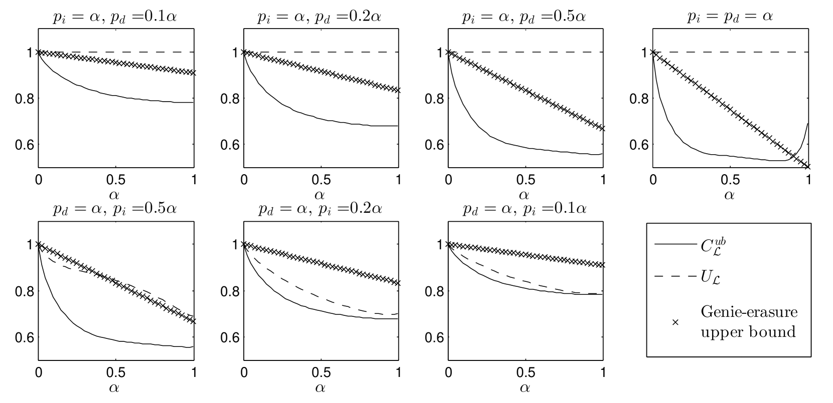
Figure 7: Comparison of the upper bounds for different $p_{i}$ and $p_{d}$. Here $\mathcal{L}=4$.

VI DID Channel Capacity at Low Noise

Observe that our bounds visually match up with one another and with the lower bound on the i.u.d. achievable rate $C_{iud}^{lb}$ (from Fig. 4) nicely for $p_{id}<0.1$. It is thus clear that for this noise range, the computed values are the true capacity. In this section, we will be interested in a finite-lettered characterization of the capacity at such low noise. Again, we will restrict the analysis to the case $p_{i}=p_{d}=p_{id}$, in particular $p_{id}<0.5$. In principle, other cases can be resolved in a similar fashion.

Along this line of work, Kanoria and Montanari [23] achieved the same goal for the deletion channel. Their approach and ours share certain similarities: both find a lower bound and an upper bound, and the lower bound is simply the achievable rate with a specific input distribution, which is the i.u.d. input. The key difference lies in the upper-bounding technique. In their analysis, first, an intermediate input distribution class is shown to yield an ``upper bound'' on the rate achieved with any input distribution; second, the rate achieved by this class is then expressed in terms of the channel parameters. The choice of the intermediate input class is not arbitrary. On one hand, properties of this class should offer sufficient analytical advantages. On the other hand, the class should be sufficiently broad so that it is possible to find an upper-bounding relation with any input distributions. Indeed the choice in [23] appears to be quite specific to the deletion channel.

In our case, it is not obvious how to pinpoint such an input class. Our problem hence calls for a different approach. Suppose that $f\left(\mu\right)$ is a good upper bound on the rate achieved by an input $\mu$. At each fixed $p_{id}$, we find the deviation $\Delta f=f\left(\mu^{*}\right)-f\left(\mu_{iud}\right)$, which results from the deviation of $\mu^{*}$, one of the capacity-achieving inputs, from $\mu_{iud}$ the i.u.d. input, via the Taylor expansion theorem. Then the order of magnitude of $\Delta f$ is evaluated w.r.t. $p_{id}$. To make this feasible, an important observation is that since we know the i.u.d. input is the only capacity-achieving input when $p_{id}=0$, $\mu^{*}\to\mu_{iud}$ as $p_{id}\to 0$. The use of $\Delta f$ hence circumvents the need for a specific intermediate input class. Note that $f$ is, strictly speaking, a function of $\mu$ and $p_{id}$. However an expansion about both $\mu_{iud}$ and $p_{id}=0$ is expected to yield the trivial rate of $1$, which is not useful. This explains why we need to treat $p_{id}$ as a fixed parameter in the expansion of $f$. Fig. 8 illustrates pictorially our strategy.

As observed from Fig. 8, the two curves close their gap and hence $\Delta f\to 0$ as $p_{id}\to 0$, which makes sense since the i.u.d. input achieves capacity at $p_{id}=0$. This is the basis for us to evaluate the order of magnitude of $\Delta f$ in terms of $p_{id}$.

Figure 8: Illustration of the low-noise calculation strategy. The upper and lower solid curves are $f$ corresponding to a capacity-achieving input and the i.u.d. input respectively. A different input deviation from the i.u.d. input would yield a different curve, e.g. the dashed curve, which may not come close to the lower solid curve as $p_{id}\to 0$.

We first define the ${\cal O}$ and $\Theta$ notations. Since $p_{id}$ is small, we say

• a quantity $Q$ scales as ${\cal O}\left(g\left(p_{id}\right)\right)$, or $Q={\cal O}\left(g\left(p_{id}\right)\right)$, if $\lim_{p_{id}\to 0}\left(\left.Q\left/g\left(p_{id}\right)\right.\right.\right)$ is finite,

• a quantity $Q$ scales as $\Theta\left(g\left(p_{id}\right)\right)$, or $Q=\Theta\left(g\left(p_{id}\right)\right)$, if $\lim_{p_{id}\to 0}\left(\left.Q\left/g\left(p_{id}\right)\right.\right.\right)$ is finite and not equal to $0$,

• a quantity $Q$ is more significant than ${\cal O}\left(g\left(p_{id}\right)\right)$ if $\lim_{p_{id}\to 0}\left(\left.Q\left/g\left(p_{id}\right)\right.\right.\right)$ is infinite.

should the limits exist.

VI-A Low-Noise Lower Bound

$C_{iud}^{lb}$ is sufficient for this purpose. The first term in $C_{iud}^{lb}$, given in Eq. (12), can be expressed as follows:

$$H\left(Y_{n}\middle|Y_{n-1},X_{n-2},Z_{n-2}\right)$$

$$=\frac{1}{4}h_{2}\left(\frac{1}{2}-\frac{1}{2}p_{id}\right)$$

$$\quad+\left(\frac{1}{2}-\frac{1}{4}p_{id}\right)h_{2}\left(\frac{1}{2}-\frac{1}{2}p_{id}+{\cal O}\left(p_{id}^{2}\right)\right)$$

$$\quad+\left(\frac{1}{4}+\frac{1}{4}p_{id}\right)h_{2}\left(\frac{1}{2}-\frac{1}{2}p_{id}+{\cal O}\left(p_{id}^{2}\right)\right)$$

$$=1+{\cal O}\left(p_{id}^{2}\right)$$

since $h_{2}\left(\frac{1}{2}+x\right)=1+\mathcal{O}\left(x^{2}\right)$. The second term, given in Eq. (13), can be shown to be more significant than ${\cal O}\left(p_{id}^{2}\right)$. Therefore, we leave the whole term as it is, and obtain the following:

$$C\geq C_{iud}^{lb}=1-\left[\sum_{k=1}^{\infty}\frac{1}{2^{k+1}}R\left(p_{id};k\right)\right]+{\cal O}\left(p_{id}^{2}\right)$$ (20)

where

$$R\left(p_{id};k\right)=h_{2}\left(\frac{1}{2}+\frac{1}{2}\left(1-2p_{id}\right)^{k}\right)$$

VI-B Low-Noise Upper Bound

$$f\left(\delta_{1},\delta_{2},p_{id}\right) =f\left(0,0,p_{id}\right)+A_{1}\left(p_{id}\right)\delta_{1}+A_{2}\left(p_{id}\right)\delta_{2}$$

$$\quad-B_{2,0}\left(c\delta_{1},c\delta_{2},p_{id}\right)\delta_{1}^{2}-2B_{1,1}\left(c\delta_{1},c\delta_{2},p_{id}\right)\delta_{1}\delta_{2}-B_{0,2}\left(c\delta_{1},c\delta_{2},p_{id}\right)\delta_{2}^{2}$$ (22)

$$f\left(0,0,p_{id}\right) =1-\left[\sum_{k=1}^{\infty}\frac{1}{2^{k+1}}R\left(p_{id};k\right)\right]+{\cal O}\left(p_{id}^{2}\right)$$

$$A_{1}\left(p_{id}\right) =\left(1-p_{id}\right)\log\frac{2-p_{id}}{2+p_{id}}-\sum_{k=1}^{\infty}\frac{k-3}{2^{k}}R\left(p_{id};k\right)$$

$$A_{2}\left(p_{id}\right) =\left(1-2p_{id}\right)\log\frac{2-p_{id}}{2+p_{id}}-\sum_{k=1}^{\infty}\frac{k-3}{2^{k}}R\left(p_{id};k\right)$$

$$B_{2,0}\left(c\delta_{1},c\delta_{2},p_{id}\right) =\frac{2\left(1-p_{id}\right)^{2}}{{\displaystyle\left[1-\left(\frac{1}{2}p_{id}+r\right)^{2}\right]}\ln 2}+\frac{1}{2}\sum_{k=1}^{\infty}q^{k-3}\left[\left(q-1\right)^{2}k^{2}+\left(q^{2}+2q-3\right)k+2\right]R\left(p_{id};k\right)$$

$$B_{0,2}\left(c\delta_{1},c\delta_{2},p_{id}\right) =\frac{2\left(1-2p_{id}\right)^{2}}{{\displaystyle\left[1-\left(\frac{1}{2}p_{id}+r\right)^{2}\right]}\ln 2}+\frac{1}{2}\sum_{k=1}^{\infty}q^{k-3}\left[\left(q-1\right)^{2}k^{2}+\left(q^{2}+2q-3\right)k+2\right]R\left(p_{id};k\right)$$

$$B_{1,1}\left(c\delta_{1},c\delta_{2},p_{id}\right) =\frac{2\left(1-p_{id}\right)\left(1-2p_{id}\right)}{{\displaystyle\left[1-\left(\frac{1}{2}p_{id}+r\right)^{2}\right]}\ln 2}+\frac{1}{2}\sum_{k=1}^{\infty}q^{k-3}\left[\left(q-1\right)^{2}k^{2}+\left(q^{2}+2q-3\right)k+2\right]R\left(p_{id};k\right)$$

$$r =2\left(1-p_{id}\right)c\delta_{1}+2\left(1-2p_{id}\right)c\delta_{2}$$

$$q =\frac{1}{2}+c\delta_{1}+c\delta_{2}$$

 

A suitable upper bound not only is sufficiently simple to analyze, but also well retains its second term $\lim_{n\to\infty}H\left(Y_{n}\middle|Y^{n-1},X^{n}\right)$ so that it can match up with the summand in Eq. (20). We now develop an upper bound with $\lim_{n\to\infty}H\left(Y_{n}\middle|Y^{n-1}\right)\leq H\left(Y_{n}\middle|Y_{n-1}\right)$, which is Eq. (17) with ${\cal L}=2$ (which should suffice since the first term on the left-hand side of this inequality decreases slowly for low $p_{id}$, as suggested by Fig. 2), while leaving the second term unchanged as before.

Let

$$p_{1} =P\left(X_{n}=X_{n-1}=X_{n-2}\right)$$

$$p_{2} =P\left(X_{n}=X_{n-1}\neq X_{n-2}\right)$$

$$p_{3} =P\left(X_{n}\neq X_{n-1}=X_{n-2}\right)$$

$$p_{4} =P\left(X_{n}=X_{n-2}\neq X_{n-1}\right)$$

The bit-symmetry condition gives us

$$P\left(X_{n-2}^{n}=000\right)= P\left(X_{n-2}^{n}=111\right)= p_{1}/2$$

$$P\left(X_{n-2}^{n}=100\right)= P\left(X_{n-2}^{n}=011\right)= p_{2}/2$$

$$P\left(X_{n-2}^{n}=110\right)= P\left(X_{n-2}^{n}=001\right)= p_{3}/2$$

$$P\left(X_{n-2}^{n}=010\right)= P\left(X_{n-2}^{n}=101\right)= p_{4}/2$$

The stationarity condition, as in Lemma 17, requires that

$$P\left(X_{n-1}^{n}=x_{1}x_{2}\right)=P\left(X_{n-2}^{n-1}=x_{1}x_{2}\right)$$

for any $x_{1},x_{2}\in\left\{0,1\right\}$, leading to $p_{2}=p_{3}$. With the fact that $p_{1}+p_{2}+p_{3}+p_{4}=1$, we are left with 2 free variables $p_{1}$ and $p_{2}$ such that $p_{4}=1-p_{1}-2p_{2}$. Then:

$$H\left(Y_{n}\middle|Y_{n-1}\right)=$$

$$h_{2}\left(\left(1-\frac{2p_{i}p_{d}}{p_{i}+p_{d}}\right)p_{1}+\left(1-\frac{4p_{i}p_{d}}{p_{i}+p_{d}}\right)p_{2}+\frac{2p_{i}p_{d}}{p_{i}+p_{d}}\right)$$

For the term $\lim_{n\to\infty}H\left(Y_{n}\middle|Y^{n-1},X_{0}^{n}\right)$, in Eq. (13), we have $\alpha=P\left(X_{n}\neq X_{n-1}\right)=1-p_{1}-p_{2}$. Let $\delta_{1}=p_{1}-\nicefrac{{1}}{{4}}$, $\delta_{2}=p_{2}-\nicefrac{{1}}{{4}}$, and

$$f\left(\delta_{1},\delta_{2},p_{id}\right)=H\left(Y_{n}\middle|Y_{n-1}\right)-{\displaystyle\lim_{n\to\infty}H\left(Y_{n}\middle|Y^{n-1},X_{0}^{n}\right)}$$

The non-negativity condition of the input distribution (i.e. $p_{1}\geq 0$, $p_{2}\geq 0$, $p_{4}=1-p_{1}-2p_{2}\geq 0$) translates to

$${\displaystyle\frac{1}{4}\geq\delta_{1}}+2\delta_{2},\quad\delta_{1}\geq-\frac{1}{4},\quad\delta_{2}\geq-\frac{1}{4}$$ (21)

The Taylor expansion theorem with Lagrange remainder applied to $f$ about the i.u.d. input (i.e. $\delta_{1}=\delta_{2}=0$) with $p_{id}$ fixed as a parameter gives Eq. (22) for some $c\in\left[0,1\right]$ (see next page). Let $\delta_{1}^{*}$ and $\delta_{2}^{*}$ be values that correspond to a capacity-achieving input. As an upper bound on the capacity $C=C\left(p_{id}\right)$ at $p_{id}$,

$$C\left(p_{id}\right)\leq f\left(\delta_{1}^{*},\delta_{2}^{*},p_{id}\right)$$

Observe that $f\left(0,0,p_{id}\right)$ matches up with $C_{iud}^{lb}$ up to ${\cal O}\left(p_{id}^{2}\right)$, which is expected for the zero-order term of a good upper bound expanded about the i.u.d. input. Therefore we only need to estimate how the rest of the terms, which represent $\Delta f$ in the opening discussion of this section, scale with $p_{id}$, without knowing their exact expression in terms of $p_{id}$.

Allowing approximations to reduce unnecessarily complex algebra and noticing that $\delta_{1}^{*}$ and $\delta_{2}^{*}$ are functions of $p_{id}$, we have:

$$A_{1}\left(p_{id}\right) \approx A_{2}\left(p_{id}\right)=A\left(p_{id}\right)$$

$$B_{2,0}\left(c\delta_{1}^{*},c\delta_{2}^{*},p_{id}\right) \approx{\displaystyle B_{0,2}\left(c\delta_{1}^{*},c\delta_{2}^{*},p_{id}\right)}$$

$$\approx{\displaystyle B_{1,1}\left(c\delta_{1}^{*},c\delta_{2}^{*},p_{id}\right)}={\displaystyle B\left(p_{id}\right)}$$

One can show that $A\left(p_{id}\right)=\Theta\left(p_{id}\right)$ with elementary calculations. The analysis of $B\left(p_{id}\right)$ requires more care, since it involves $\delta_{1}^{*}$ and $\delta_{2}^{*}$. Let $b_{1}\left(p_{id}\right)$ denote the first term in $B\left(p_{id}\right)$, i.e.

$$b_{1}\left(p_{id}\right)=\frac{2\left(1-p_{id}\right)\left(1-2p_{id}\right)}{{\displaystyle\left[1-\left(\frac{1}{2}p_{id}+r^{*}\right)^{2}\right]}\ln 2}$$

where $r^{*}=2\left(1-p_{id}\right)c\delta_{1}^{*}+2\left(1-2p_{id}\right)c\delta_{2}^{*}$, and $b_{2}\left(p_{id}\right)=B\left(p_{id}\right)-b_{1}\left(p_{id}\right)$. For $\delta_{1}^{*}$ and $\delta_{2}^{*}$ under the constraint (21) and $p_{id}<0.5$, noticing that $\delta_{1}^{*}$ and $\delta_{2}^{*}$ approach $0$ as $p_{id}\to 0$, one can see easily that $b_{1}\left(p_{id}\right)>0$ and $b_{1}\left(p_{id}\right)=\Theta\left(1\right)$. Also, $b_{1}\left(p_{id}\right)$ is undefined if and only if $c=1$, $\delta_{1}^{*}=0.75$ and $\delta_{2}^{*}=-0.25$, in which case the capacity-achieving input only allows the all-zeros and all-ones input strings and hence the capacity is trivially $0$. However $C_{iud}^{lb}$ is always away from $0$ for any $p_{id}$. We therefore exclude such large deviations from $0$ of $\delta_{1}^{*}$ and $\delta_{2}^{*}$.

To evaluate $b_{2}\left(p_{id}\right)$, we first note that $q^{*}=\frac{1}{2}+c\delta_{1}^{*}+c\delta_{2}^{*}\in\left[0,1\right]$ under the constraint (21). $q^{*}=1$ if and only if $c=1$, $\delta_{1}^{*}=0.75$ and $\delta_{2}^{*}=-0.25$. So for the same reason above, we can bound $q^{*}\leq\epsilon<1$. In addition, since $q^{*}$ is finite, there exists a polynomial $P_{2}\left(k\right)$ of degree $2$ over the real numbers such that $P_{2}\left(k\right)\geq\left|\left(q^{*}-1\right)^{2}k^{2}+\left(q^{*2}+2q^{*}-3\right)k+2\right|$ for any $k\geq 1$. Letting $M_{k}=\epsilon^{k-3}P_{2}\left(k\right)$, we then have $M_{k}\geq\left|q^{*k-3}\left[\left(q^{*}-1\right)^{2}k^{2}+\left(q^{*2}+2q^{*}-3\right)k+2\right]R\left(p_{id};k\right)\right|$ for any $p_{id}$, since $\left|R\left(p_{id};k\right)\right|\leq 1$. We also have that $\sum_{k=1}^{\infty}M_{k}$ converges as a straightforward application of the ratio test for series convergence. Then by the Weierstrass M-test, we have that $b_{2}\left(p_{id}\right)$ converges uniformly. Consequently,

$$\lim_{p_{id}\to 0}b_{2}\left(p_{id}\right)$$

$$=\frac{1}{2}\sum_{k=1}^{\infty}\lim_{p_{id}\to 0}\left\{\begin{array}[]{c}q^{*k-3}R\left(p_{id};k\right)\times\\ \left[\left(q^{*}-1\right)^{2}k^{2}+\left(q^{*2}+2q^{*}-3\right)k+2\right]\end{array}\right\}$$

$$=0$$

That is, $b_{2}\left(p_{id}\right)={\cal O}\left(1\right)$ (and in fact, of order of magnitude much lesser than $\Theta\left(1\right)$).

As a result, $B\left(p_{id}\right)=\Theta\left(1\right)$ for $p_{id}<0.5$. Since $b_{2}\left(p_{id}\right)\ll b_{1}\left(p_{id}\right)$ and $b_{1}\left(p_{id}\right)>0$, we can conclude that $B\left(p_{id}\right)>0$ at sufficiently low $p_{id}$. In fact, Fig. 9 suggests that $B\left(p_{id}\right)$ is potentially non-positive only in extreme cases where $p_{id}$ is close to $0.5$, $\delta_{1}^{*}$ is close to $0.75$ and $\delta_{2}^{*}$ is close to $-0.25$. For the purpose of obtaining low-noise approximations, we can therefore say that $B\left(p_{id}\right)>0$. We then have:

$$C\left(p_{id}\right)-f\left(0,0,p_{id}\right)$$

$$\leq f\left(\delta_{1}^{*},\delta_{2}^{*},p_{id}\right)-f\left(0,0,p_{id}\right)$$

$$\approx\left(\delta_{1}^{*}+\delta_{2}^{*}\right)A\left(p_{id}\right)-\left(\delta_{1}^{*}+\delta_{2}^{*}\right)^{2}B\left(p_{id}\right)$$

$$\leq\sup_{t\in\mathbb{R}}\left[tA\left(p_{id}\right)-t^{2}B\left(p_{id}\right)\right]$$

$$=\frac{A^{2}\left(p_{id}\right)}{4B\left(p_{id}\right)}=\Theta\left(p_{id}^{2}\right)$$ (23)

using the identity $\sup_{t\in\mathbb{R}}\left(at^{2}+bt+c\right)=\left(4ac-b^{2}\right)/\left(4a\right)$ for $a<0$. This completes the derivation of the low-noise upper bound.

The same conclusion, $C\left(p_{id}\right)\leq f\left(0,0,p_{id}\right)+\Theta\left(p_{id}^{2}\right)$, can be reached without the approximations by doing some tedious algebra. Approximations do not affect our result anyway, since in this analysis only the order of magnitude of $A\left(p_{id}\right)$ and $B\left(p_{id}\right)$ matters. We also see that $\Delta f$ in the opening discussion corresponds to $\Theta\left(p_{id}^{2}\right)$, which tends to $0$ as $p_{id}\to 0$. This concurs with the discussed observation from Fig. 8.

As a note, it is clear why the expansion of $f$ is up to the second order. The first-order expansion would make the supremum in our final step unbounded, while any higher-order expansions would complicate the analysis.

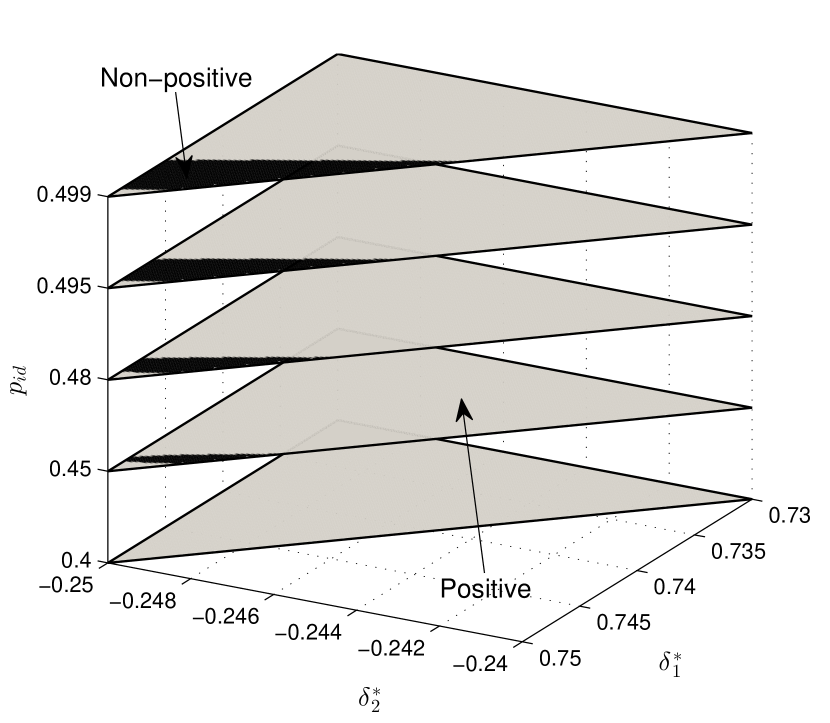
Figure 9: Sign of $B\left(p_{id}\right)$ for different values of $p_{id}$, $\delta_{1}^{*}$ and $\delta_{2}^{*}$, which satisfy the constraint (21). The summands of $b_{2}\left(p_{id}\right)$ are limited to a maximum $k$ of $2000$ for computational feasibility. In general, the ``non-positive'' region shrinks as the maximum $k$ is increased. Here $c$ is set to $1$. However this particular choice of $c$ is irrelevant, since values of $B\left(p_{id}\right)$ with $\left(c,\delta_{1}^{*},\delta_{2}^{*}\right)=\left(c^{\prime},d_{1},d_{2}\right)$, where $c^{\prime}<1$, are equal to those with $\left(c,\delta_{1}^{*},\delta_{2}^{*}\right)=\left(1,c^{\prime}d_{1},c^{\prime}d_{2}\right)$.

VI-C Low-Noise Characterization of the Capacity

Putting Eq. (20) and (23) together,

$$C=1-\left[\sum_{k=1}^{\infty}\frac{1}{2^{k+1}}R\left(p_{id};k\right)\right]+{\cal O}\left(p_{id}^{2}\right)$$

This characterization, ignoring ${\cal O}\left(p_{id}^{2}\right)$, is plotted in Fig. 10.

It can be easily shown that $R\left(p_{id};k\right)$ is concave in $p_{id}$ for every $k\geq 1$ and $p_{id}\in\left(0,0.5\right)$. Therefore this analysis suggests that the capacity is a convex function of the channel parameter $p_{id}$ in the low-noise regime.

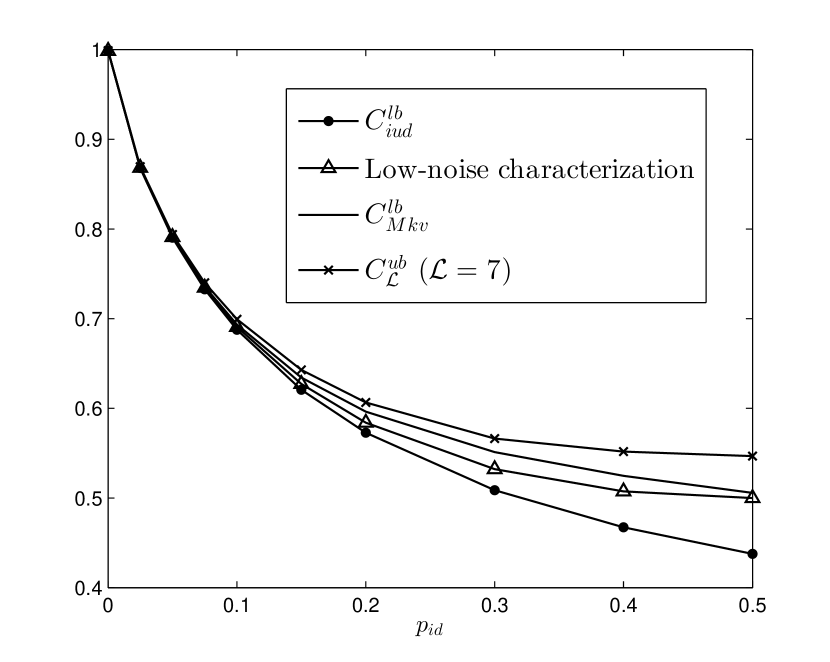
Figure 10: The DID channel capacity at low noise.

VII Concluding Remarks

This work has illustrated the use of the stationarity condition of the supremizing input set in the capacity formula in a case study of the DID channel model. Input stationarity has been identified in both ergodic-theoretic and Shannon-theoretic capacity formulations. Evidently this condition is pivotal to many of our results. Without it, the new upper bounds could become trivial as discussed in Section V-C. Moreover this condition helps describe finite-dimensional marginal distributions $P_{X_{n+a}^{n+b}}$, with $a\leq b$, for all $n$'s in only a finite number of variables, which is key to establishing Lemma 15 and subsequently the low-noise characterization.

Our simultaneous treatment of the two separate, seemingly unrelated frameworks is necessary. Input stationarity arises naturally in the ergodic-theoretic framework. The reason is that this framework allows only infinitely long input sequences, an example of whose source is stationary inputs. On the contrary, in the Shannon-theoretic framework, allowable input sequences have finite (block) lengths, and only when reliable communications is of concern (i.e. the error probability is driven to zero) are the block lengths increased to infinity. This setting makes it harder to see whether stationary inputs and the likes should play any role in capacity formulations. As witnessed in Section III-D, via a connection to results in the ergodic-theoretic framework, developments to a formulation with stationary inputs could be realized. With further scrutiny, one sees that the difference between the two frameworks lies mainly in their operational structures, whereas the said connection is purely on information-theoretic quantities, which are dictated by the joint input-output distribution, shared by both frameworks. Curiously the Shannon-theoretic framework is not the only beneficiary. An argument in Appendix A shows that so is the ergodic-theoretic framework.

Next we discuss a few relevant directions concerning the capacity evaluation techniques for further investigations.

Channels with High Local Dependency

The DID channel output has relatively low local dependency: $Y_{i}$ is determined only through the present and the immediate past, $\left\{Z_{i},X_{i-1}^{i}\right\}$. This may give an intuitive explanation of why the upper bounds in Fig. 5 converge very quickly at low $\mathcal{L}$.

We however cannot expect this to be the case for other practical channels, e.g. the model in [10]. As mentioned in Section I-C, the DID channel only captures partially key features of the BPMR write process. For example, it can be observed that in the DID channel model, an output sub-sequence either remains synchronized with its corresponding input sub-sequence or leads it by $1$ bit. The scenario in which the output sub-sequence lags behind the input sub-sequence by $1$ bit is therefore missing. This was considered by the model in [10], which sets the alphabet of $Z_{i}$ to ${\cal Z}=\left\{-1,0,1\right\}$. While such ${\cal{\cal Z}}$ makes the channel non-causal, one can redefine the input to be $\hat{X}_{i}=X_{i-1}$ and consequently $Y_{i}=\hat{X}_{i+1-Z_{i}}$, which is a mathematically causal channel and to which Eq. (8) is again applicable. The scenario where misalignment by more than $1$ bit is allowed was discussed in [8, Section VI], in which case ${\cal Z}$ also has larger sizes.

All those considerations lead to higher local dependency, which gives rise to numerous difficulties. At first glance, the convergence would be slower. To resolve this, one may increase $\mathcal{L}$ (or some similar parameters that control the bounds) to obtain the desired accuracy to the true capacity. However the larger ${\cal L}$ is, higher the computational complexity. The intrinsic tradeoff between accuracy and complexity is therefore more stringent in this case, which may call for a modification or a different formulation of the upper bound.

Channels with Substitution Errors

Substitution errors are usually inevitable in practical systems. For example, it was noted in [10] that insertion and deletion errors, underlied by the Markov channel state $\left\{Z_{i}\right\}_{i=1}^{\infty}$, are not sufficient to faithfully describe all imperfections that arise in the context of BPMR. Their model considered burst substitution errors that accompany insertion and deletion events, in addition to random substitution errors caused by a localized random phase drift between the desired and actual window to write each bit.

In general, we may model substitution errors by $Y_{i}=X_{i-Z_{i}}\oplus B_{i}$, where $B_{i}$ is a binary random variable representing the additive noise, independent of the input. A straightforward approach is to take into account $B_{i}$ and do the exact calculation. Another way is to view the model as two subsystems, in which one is $A_{i}=X_{i-Z_{i}}$, concatenated with the other $Y_{i}=A_{i}\oplus B_{i}$. Then an upper bound on the capacity is given by the data processing inequality, $I\left(\mathbf{X};\mathbf{Y}\right)\leq\min\left\{I\left(\mathbf{X};\mathbf{A}\right),I\left(\mathbf{A};\mathbf{Y}\right)\right\}$, suggesting that $C\leq\min\left\{C_{1},C_{2}\right\}$, where $C$, $C_{1}$ and $C_{2}$ are the true capacity, the first subsystem's capacity and that of the second subsystem respectively. This gives a simple benchmark upper bound.

Finite-Block-Length Regime

One natural question is how the fundamental limit behaves when the block length is finite (see e.g. [24, 25]). In this analysis, the capacity is known as the first-order coding rate, and the quest is to find higher-order coding rates given a finite block length $n$ and some non-zero tolerable error probability $\epsilon$. Note that the finite-block-length analysis is usually developed under the Shannon-theoretic framework. It is unclear how the ergodic-theoretic channel definition could extend itself to encompass finite block lengths.

While finite-lettered characterizations of the second-order coding rate have been determined precisely for certain channels, they are not known in general for channels with memory or complex structures. Since the DID channel's first-order coding rate has been determined approximately under the Shannon-theoretic framework as discussed above, it would be interesting to see how one can approximate its second-order coding rate as a series expansion in the channel parameters.

Appendix A

We consider the ergodic-theoretic ``capacity'' formulation with general initializations of the state $Z_{1}$. The DID channel is an FSC in the Shannon-theoretic framework. It was pointed out by Kieffer and Rahe [26] (and also by Gray et al. [27]) that FSCs can be naturally described as a special case of (one-sided) Markov channels in the ergodic-theoretic setting. Furthermore they showed that Markov channels are asymptotically mean stationary (AMS). Hence so is the DID channel.

For any $p_{i}$ and $p_{d}$ in $\left(0,1\right)$, the process $\left\{Z_{i}\right\}_{i=1}^{\infty}$ is mixing. As such, the DID channel is output strongly mixing, in light of Section II-A. Since the channel is (one-sided) Markov, by [27, Theorem 2] and [27, Lemma 3], it is ergodic.

By [5, Theorem 12.6.1], the following rate is achievable:

$$C^{*}\left(P_{\mathbf{Z}}\right) =\sup_{\text{AMS }P_{X_{0}^{\infty}}}\lim_{n\to\infty}\frac{1}{n}I_{AMS}\left(X_{0}^{n};Y_{1}^{n}\right)$$ (24)

Here the subscript $AMS$ means that it is calculated w.r.t. the stationary mean of the joint input-output distribution, and the notation $C^{*}\left(P_{\mathbf{Z}}\right)$ emphasizes the dependence of the rate on the distribution $P_{\mathbf{Z}}$ of the process $\left\{Z_{i}\right\}_{i=1}^{\infty}$.

All that is left is to establish an equality between Eq. (6) (which assumes $P\left(Z_{1}=0\right)=p_{d}/\left(p_{i}+p_{d}\right)$ and $P\left(Z_{1}=1\right)=p_{i}/\left(p_{i}+p_{d}\right)$) and Eq. (24). We digress from the task temporarily. The notion of AMS processes does not closely describe the processes associated with the DID channel. We hence appeal to the following definition.

Definition 18.

A random process $\{V_{n}\}_{n=1}^{\infty}$, defined over a probability space $(\Omega,\mathcal{F},P)$, is asymptotically stationary (AS) if $\forall E\in\mathcal{F}$, the limit $P^{\infty}(E)=\lim_{n\rightarrow\infty}P(T^{-n}E)$ exists. $P^{\infty}$ is then called the asymptotic stationary probability measure.

One can easily prove that a stationary measure is AS and AMS. In addition, we have the following lemma.

Lemma 19.

An AS process is AMS. Furthermore, the stationary mean is its asymptotic stationary probability measure.

Proof:

The claim follows easily from the definitions and the Cesàro mean theorem. ∎

Consider two independent processes $\{A_{n}\}_{n=1}^{\infty}$ and $\{B_{n}\}_{n=1}^{\infty}$, whose underlying probability measures are respectively $P_{A}$ and $P_{B}$. Let $P_{AB}$ denote the probability measure of the joint process $\left\{\left(A_{n},B_{n}\right)\right\}_{n=1}^{\infty}$. For any event $E$ on this joint process, we have:

$$P_{AB}\left(T^{-n}E\right) =\intop_{\left(\mathbf{a},\mathbf{b}\right)\in E}\sum_{\begin{subarray}{c}\mathbf{a}^{\prime}\in{\cal A}^{n}\\ \mathbf{b}^{\prime}\in{\cal B}^{n}\end{subarray}}dP_{AB}\left(\left[\mathbf{a}^{\prime},\mathbf{a}\right],\left[\mathbf{b}^{\prime},\mathbf{b}\right]\right)$$

$$=\intop_{\left(\mathbf{a},\mathbf{b}\right)\in E}\sum_{\begin{subarray}{c}\mathbf{a}^{\prime}\in{\cal A}^{n}\\ \mathbf{b}^{\prime}\in{\cal B}^{n}\end{subarray}}d\left(P_{A}\times P_{B}\right)\left(\left[\mathbf{a}^{\prime},\mathbf{a}\right],\left[\mathbf{b}^{\prime},\mathbf{b}\right]\right)$$

$$=\intop_{\left(\mathbf{a},\mathbf{b}\right)\in E}d\left(P_{A}\times P_{B}\right)\left(T^{-n}\left\{\mathbf{a}\right\},T^{-n}\left\{\mathbf{b}\right\}\right)$$

This shows that if $\{A_{n}\}_{n=1}^{\infty}$ and $\{B_{n}\}_{n=1}^{\infty}$ are AS, $\left\{\left(A_{n},B_{n}\right)\right\}_{n=1}^{\infty}$ is also AS. Moreover $P_{AB}^{\infty}$ is determined completely by $P_{A}^{\infty}$ and $P_{B}^{\infty}$, which denote the associated asymptotic stationary probability measures.

Next, consider a process $\{V_{n}\}_{n=1}^{\infty}$, defined under $P_{V}$. Define another process $\{W_{n}:\;W_{n}=\phi(V_{n},V_{n-1},...,V_{n-k})\}$, where $\phi$ is a deterministic and time-invariant function and $k$ is finite. Let $P_{W}$ be the underlying probability measure of $\{W_{n}\}_{n=k+1}^{\infty}$, and consider an event $E_{W}$ on the process. Let $\mathcal{E}_{i}=\left\{u_{i}:\;\mathbf{u}\in E_{W}\right\}$. Let $E_{W}^{i}=\left\{\mathbf{w}:\;w_{i}\in\mathcal{E}_{i}\right\}$ and $E_{V}^{i}=\left\{\mathbf{v}:\;\phi\left(v_{i-k}^{i}\right)\in\mathcal{E}_{i}\right\}$. Then for any $j\geq 0$:

$$P_{W}\left(T^{-j}E_{W}\right) =P_{W}\left(T^{-j}\bigcap_{i=k+1}^{\infty}E_{W}^{i}\right)$$

$$=P_{W}\left(\bigcap_{i=k+1}^{\infty}\left\{\mathbf{w}:\;w_{i+j}\in\mathcal{E}_{i}\right\}\right)$$

$$=P_{V}\left(\bigcap_{i=k+1}^{\infty}\left\{\mathbf{v}:\;\phi\left(v_{i+j-k}^{i+j}\right)\in\mathcal{E}_{i}\right\}\right)$$

$$=P_{V}\left(T^{-j}\bigcap_{i=k+1}^{\infty}E_{V}^{i}\right)$$

where the third equality is because firstly, any $\mathbf{v}\in\bigcap_{i=k+1}^{\infty}\left\{\mathbf{v}:\;\phi\left(v_{i+j-k}^{i+j}\right)\in\mathcal{E}_{i}\right\}$, under $\phi$, is transformed into some $\mathbf{w}\in\bigcap_{i=k+1}^{\infty}\left\{\mathbf{w}:\;w_{i+j}\in\mathcal{E}_{i}\right\}$, and secondly, for any $\mathbf{v}\notin\bigcap_{i=k+1}^{\infty}\left\{\mathbf{v}:\;\phi\left(v_{i+j-k}^{i+j}\right)\in\mathcal{E}_{i}\right\}$, there exists at least one index $r\geq k+1$ such that $\phi\left(v_{r+j-k}^{r+j}\right)\notin\mathcal{E}_{r}$ and so $\mathbf{v}$ is not transformed into any member of $\bigcap_{i=k+1}^{\infty}\left\{\mathbf{w}:\;w_{i+j}\in\mathcal{E}_{i}\right\}$. This shows that if $\{V_{n}\}_{n=1}^{\infty}$ is AS, so is $\{W_{n}\}_{n=k+1}^{\infty}$. Moreover $P_{W}^{\infty}$ is completely determined by $P_{V}^{\infty}$.

We return to our original problem. Consider AMS $P_{X_{0}^{\infty}}$, since Eq. (24) involves only AMS inputs. It is known that $\{Z_{i}\}_{i=1}^{\infty}$ is AS for any $p_{i},p_{d}\in\left(0,1\right)$; moreover it has a unique $P_{\mathbf{Z}}^{\infty}$ which coincides with its distribution $P_{\mathbf{Z}}^{*}$ when $P\left(Z_{1}=0\right)=p_{d}/\left(p_{i}+p_{d}\right)$ and $P\left(Z_{1}=1\right)=p_{i}/\left(p_{i}+p_{d}\right)$, i.e. when the initialization allows it to be stationary, for the same $p_{i}$ and $p_{d}$. Notice that for the DID channel, we can express $\left(X_{i},Y_{i}\right)$ as deterministic and time-invariant functions of $\left(\left(X_{i},X_{i-1}\right),Z_{i}\right)$. Let $\left(X_{i},X_{i-1}\right)$, $Z_{i}$, $\left(\left(X_{i},X_{i-1}\right),Z_{i}\right)$ and $\left(X_{i},Y_{i}\right)$ play the role of $A_{i}$, $B_{i}$, $V_{i}$ and $W_{i}$, respectively, in the above discussion. We see that the joint input-output distribution is AS. By Lemma 19, this implies that $C^{*}\left(P_{\mathbf{Z}}\right)$ can be computed w.r.t. $P_{X^{\infty}\mathbf{Y}}^{\infty}$. Furthermore $P_{X^{\infty}\mathbf{Y}}^{\infty}$ is completely determined by the input distribution, which is AMS, and $P_{\mathbf{Z}}^{\infty}$, which is the same as $P_{\mathbf{Z}}^{*}$. Therefore, instead of using the channel law in Eq. (5) which asserts

$$P_{\left.\mathbf{Y}\middle|X_{0}^{\infty}\right.}\left(E_{Y}\middle|\mathbf{x}\right)=P_{\mathbf{Z}}\left({\cal E}\left(\mathbf{x},E_{Y}\right)\right)$$

we can compute $C^{*}\left(P_{\mathbf{Z}}\right)$ as if the channel law is

$$P_{\left.\mathbf{Y}\middle|X_{0}^{\infty}\right.}\left(E_{Y}\middle|\mathbf{x}\right)=P_{\mathbf{Z}}^{*}\left({\cal E}\left(\mathbf{x},E_{Y}\right)\right)$$

i.e. $C^{*}\left(P_{\mathbf{Z}}\right)=C^{*}\left(P_{\mathbf{Z}}^{*}\right)$. When the channel assumes $P_{\mathbf{Z}}^{*}$, it is stationary as shown in Section II-A. By [5, Lemma 12.4.2],

$$C^{*}\left(P_{\mathbf{Z}}^{*}\right) =\sup_{\text{Stationary }P_{X_{0}^{\infty}}}\lim_{n\to\infty}\frac{1}{n}I\left(X_{0}^{n};Y_{1}^{n}\right)$$

whose right-hand side coincides with that of Eq. (6). This completes our argument.

Appendix B

We prove Theorem 11. As a reminder, this proof is under the Shannon-theoretic framework.

Lemma 20.

The SE capacity of a consistent SE channel with finite alphabets is given by

$$C_{SE}=\sup_{\text{SE }\left\{X_{1-\lambda_{-}}^{n+\lambda_{+}}\right\}_{n=1}^{\infty}}\lim_{n\to\infty}\frac{1}{n}I\left(X_{1-\lambda_{-}}^{n+\lambda_{+}};Y^{n}\right)$$

Proof:

Given any SE input, a single joint distribution $P_{X_{1-\lambda_{-}}^{\infty}\mathbf{Y}}$ exists and is SE. With an abuse of notation, we therefore drop all subscripts and use $p$ to denote the respective probability measure. Let $W_{n}=\left(Y_{n},X_{n-\lambda_{-}}^{n+\lambda_{+}}\right)$; then $\left\{W_{n}\right\}_{n=1}^{\infty}$ is SE.

$$\frac{1}{n}i^{\left(n\right)}\left(X_{1-\lambda_{-}}^{n+\lambda_{+}};Y^{n}\right)$$

$$=\frac{1}{n}\log p\left(W^{n}\right)-\frac{1}{n}\log p\left(X_{1-\lambda_{-}}^{n+\lambda_{+}}\right)-\frac{1}{n}\log p\left(Y^{n}\right)$$

$$\xrightarrow{n\to\infty}-\lim_{n\to\infty}\frac{1}{n}H\left(W^{n}\right)+\lim_{n\to\infty}\frac{1}{n}H\left(X_{1-\lambda_{-}}^{n+\lambda_{+}}\right)$$

$$\qquad\quad+\lim_{n\to\infty}\frac{1}{n}H\left(Y^{n}\right)$$

$$=\lim_{n\to\infty}\frac{1}{n}I\left(X_{1-\lambda_{-}}^{n+\lambda_{+}};Y^{n}\right)$$

where the convergence is almost-sure in $P_{X_{1-\lambda_{-}}^{\infty}\mathbf{Y}}$, by invoking the Shannon-McMillan-Breiman theorem. Since $\underline{\mathbf{I}}\left(\mathbf{X};\mathbf{Y}\right)$ is the left end point of the support of the distribution of $\frac{1}{n}i^{\left(n\right)}\left(X_{1-\lambda_{-}}^{n+\lambda_{+}};Y^{n}\right)$ at the limit $n\to\infty$, this convergence implies the claim. ∎

The main proof is a modification of Feinstein's work [15], which is under the ergodic-theoretic framework. We exploit his construction of an SE probability measure from a finite-dimensional probability measure. For some fixed $r\in\mathbb{N}^{+}$ and $s=r+\lambda_{+}+\lambda_{-}$, let us consider an arbitrary probability measure $P^{\left(r\right)}$ of $X_{1-\lambda_{-}}^{r+\lambda_{+}}$. Define a probability measure $\mu$ such that for any two integers $k_{1}$ and $k_{2}$ where $0\leq k_{1}<k_{2}$:

$$\mu\left(X_{k_{1}s+1-\lambda_{-}}^{k_{2}s-\lambda_{-}}=x_{k_{1}s+1}^{k_{2}s}\right)=\prod_{k=k_{1}}^{k_{2}-1}P^{\left(r\right)}\left(x_{ks+1}^{\left(k+1\right)s}\right)$$

It is easy to see that $\mu$ is $s$-stationary. Let us define another probability measure $\hat{\mu}$ such that for any event $E$ on the input:

$$\hat{\mu}\left(E\right)=\frac{1}{s}\left[\mu_{0}\left(E\right)+\mu_{1}\left(E\right)+...+\mu_{s-1}\left(E\right)\right]$$

where $\mu_{k}$ is defined by $\mu_{k}\left(E\right)=\mu\left(T^{-k}E\right)$ $\forall E$, for $k=0,\ldots,s-1$. It can be easily established in a similar manner to [15] that $\hat{\mu}$ is SE. Then we immediately see that $\mu$ is ergodic, since for any invariant event $E$, $\mu\left(E\right)=\hat{\mu}\left(E\right)$, which is equal to either $0$ or $1$.

We shall need the following lemma.

Lemma 21.

For any four random variables $X_{1}$, $X_{2}$, $Y_{1}$ and $Y_{2}$, in which $X_{1}$ is independent of $X_{2}$, we have:

$$I\left(X_{1},X_{2};Y_{1},Y_{2}\right)\geq I\left(X_{1};Y_{1}\right)+I\left(X_{2};Y_{2}\right)$$

Proof:

This lemma can be found in [28, Problem 2.4(e)]. We provide a proof here for completeness.

$$I\left(X_{1},X_{2};Y_{1},Y_{2}\right)$$

$$=I\left(X_{1};Y_{1},Y_{2}\right)+I\left(X_{2};Y_{1},Y_{2}\middle|X_{1}\right)$$

$$=I\left(X_{1};Y_{1},Y_{2}\right)+I\left(X_{2};Y_{1},Y_{2},X_{1}\right)-I\left(X_{1};X_{2}\right)$$

$$=I\left(X_{1};Y_{1},Y_{2}\right)+I\left(X_{2};Y_{1},Y_{2},X_{1}\right)$$

$$\geq I\left(X_{1};Y_{1}\right)+I\left(X_{2};Y_{2}\right)$$

where $I\left(X_{1};X_{2}\right)=0$ since $X_{1}$ and $X_{2}$ are independent. ∎

Proof:

Let us consider an arbitrary finite-dimensional distribution sequence $\left\{P^{\left(n\right)}\right\}_{n=1}^{\infty}$, which should be understood as an arbitrary input sequence and is not necessarily consistent, and some $r\in\mathbb{N}^{+}$. We construct the aforementioned probability measures $\mu$ and $\hat{\mu}$ from $P^{\left(r\right)}$. By passing the input generated by $\mu$ (resp. $\hat{\mu}$) through the channel, we obtain the joint input-output distribution $\omega$ (resp. $\hat{\omega}$) and the output distribution $\eta$ (resp. $\hat{\eta}$). A single measure $\omega$ (resp. $\hat{\omega}$) exists, and consequently $\eta$ (resp. $\hat{\eta}$) exists, since the channel is consistent. Since the relations are linear,

$$\hat{\omega} =\frac{1}{s}\left(\omega_{0}+\omega_{1}+...+\omega_{s-1}\right)$$

$$\hat{\eta} =\frac{1}{s}\left(\eta_{0}+\eta_{1}+...+\eta_{s-1}\right)$$

where $\omega_{k}$ and $\eta_{k}$ are the distributions corresponding to the input $\mu_{k}$, for $k=0,\ldots,s-1$. It is easy to see that $\mu_{k}$ is $s$-stationary since $\mu$ is $s$-stationary. Therefore $\omega_{k}$ and $\eta_{k}$ are $s$-stationary, since the channel is weakly stationary. Notice the following:

$$\omega_{k}\left(X_{1-\lambda_{-}}^{n+\lambda_{+}}=\mathbf{x},Y^{n}=\mathbf{y}\right)$$

$$=P_{\left.Y^{n}\middle|X_{1-\lambda_{-}}^{n+\lambda_{+}}\right.}\left(\mathbf{y}\middle|\mathbf{x}\right)\mu_{k}\left(X_{1-\lambda_{-}}^{n+\lambda_{+}}=\mathbf{x}\right)$$

$$=\sum_{\mathbf{\tilde{x}\in{\cal X}^{k}}}P_{\left.Y^{n}\middle|X_{1-\lambda_{-}}^{n+\lambda_{+}}\right.}\left(\mathbf{y}\middle|\mathbf{x}\right)\mu\left(\left\{X_{1-\lambda_{-}}^{n+k+\lambda_{+}}=\left[\mathbf{\tilde{x}},\mathbf{x}\right]\right\}\right)$$

$$\stackrel{{\scriptstyle\left(a\right)}}{{=}}\sum_{\mathbf{\tilde{x}\in{\cal X}^{k}}}P_{\left.Y^{n+k}\middle|X_{1-\lambda_{-}}^{n+k+\lambda_{+}}\right.}\left(\left\{Y_{k+1}^{n+k}=\mathbf{y}\right\}\middle|\left[\mathbf{\tilde{x}},\mathbf{x}\right]\right)$$

$$\qquad\qquad\times\mu\left(\left\{X_{1-\lambda_{-}}^{n+k+\lambda_{+}}=\left[\mathbf{\tilde{x}},\mathbf{x}\right]\right\}\right)$$

$$=\omega\left(T^{-k}\left\{X_{1-\lambda_{-}}^{n+\lambda_{+}}=\mathbf{x},Y^{n}=\mathbf{y}\right\}\right)$$

where $\left(a\right)$ is because the channel is stationary. This implies that $\omega_{k}=\omega T^{-k}$ and consequently $\eta_{k}=\eta T^{-k}$.

With these facts, similar to [15], one can prove the following limits exist:

$${\displaystyle\lim_{n\rightarrow\infty}\frac{1}{n}H_{\hat{\mu}}\left(X_{1-\lambda_{-}}^{n+\lambda_{+}}\right)} ={\displaystyle\lim_{n\rightarrow\infty}\frac{1}{n}H_{\mu}\left(X_{1-\lambda_{-}}^{n+\lambda_{+}}\right)}$$

$${\displaystyle\lim_{n\rightarrow\infty}\frac{1}{n}H_{\hat{\omega}}\left(X_{1-\lambda_{-}}^{n+\lambda_{+}},Y^{n}\right)} ={\displaystyle\lim_{n\rightarrow\infty}\frac{1}{n}H_{\omega}\left(X_{1-\lambda_{-}}^{n+\lambda_{+}},Y^{n}\right)}$$

$${\displaystyle\lim_{n\rightarrow\infty}\frac{1}{n}H_{\hat{\eta}}\left(Y^{n}\right)} =\lim_{n\rightarrow\infty}\frac{1}{n}H_{\eta}\left(Y^{n}\right)$$

and consequently,

$$\lim_{n\rightarrow\infty}\frac{1}{n}I_{\hat{\mu}}\left(X_{1-\lambda_{-}}^{n+\lambda_{+}};Y^{n}\right)=\lim_{n\rightarrow\infty}\frac{1}{n}I_{\mu}\left(X_{1-\lambda_{-}}^{n+\lambda_{+}};Y^{n}\right)$$

where the probability measure subscript in the entropy quantity implies that the quantity is calculated w.r.t. that measure, and that in the mutual information quantity implies the ``rate'' achieved by using the respective measure as the input distribution. The superscript $\left(n\right)$ is dropped without ambiguity.

Without loss of generality, let $n=ts-\lambda_{+}-\lambda_{-}$, in which $t\rightarrow\infty$. Notice that, due to the structure of $\mu$, the blocks $\left\{X_{(i-1)s+1-\lambda_{-}}^{is-\lambda_{-}}\right\}_{i=1}^{t}$ are independent of each other under $\mu$. Then:

$$\frac{1}{n}I_{\mu}\left(X_{1-\lambda_{-}}^{n+\lambda_{+}};Y^{n}\right)$$

$$\geq\frac{1}{n}I_{\mu}\left(X_{1-\lambda_{-}}^{ts-\lambda_{-}};Y_{1}^{r},Y_{s+1}^{s+r},\ldots,Y_{\left(t-1\right)s+1}^{\left(t-1\right)s+r}\right)$$

$$\stackrel{{\scriptstyle\left(a\right)}}{{\geq}}\frac{1}{n}\sum_{i=1}^{t}I_{\mu}\left(X_{\left(i-1\right)s+1-\lambda_{-}}^{is-\lambda_{-}};Y_{\left(i-1\right)s+1}^{\left(i-1\right)s+r}\right)$$

$$\stackrel{{\scriptstyle\left(b\right)}}{{=}}\frac{t}{n}I_{\mu}\left(X_{1-\lambda_{-}}^{r+\lambda_{+}};Y_{1}^{r}\right)$$

$$\stackrel{{\scriptstyle\left(c\right)}}{{=}}\frac{t}{n}I^{\left(r\right)}\left(X_{1-\lambda_{-}}^{r+\lambda_{+}};Y_{1}^{r}\right)$$

$$\geq\frac{1}{r+\lambda_{+}+\lambda_{-}}I^{\left(r\right)}\left(X_{1-\lambda_{-}}^{r+\lambda_{+}};Y_{1}^{r}\right)$$

Here $\left(a\right)$ is by applying repeatedly Lemma 21; $\left(b\right)$ is because the channel is weakly stationary, $\mu$ is $s$-stationary and consequently $\omega$ is $s$-stationary; $\left(c\right)$ is due to the fact that the distribution of $X_{1-\lambda_{-}}^{r+\lambda_{+}}$ under $\mu$ is simply $P^{\left(r\right)}$ and the channel is consistent.

Next we indicate the choice of $r$. We have $\forall\epsilon>0$, there exists $r=r\left(\epsilon\right)$ such that

$$\frac{1}{r+\lambda_{+}+\lambda_{-}}I^{\left(r\right)}\left(X_{1-\lambda_{-}}^{r+\lambda_{+}};Y_{1}^{r}\right)$$

$$\geq\liminf_{N\rightarrow\infty}\frac{1}{N+\lambda_{+}+\lambda_{-}}I^{\left(N\right)}\left(X_{1-\lambda_{-}}^{N+\lambda_{+}};Y^{N}\right)-\epsilon$$

$$=\liminf_{N\rightarrow\infty}\frac{1}{N}I^{\left(N\right)}\left(X_{1-\lambda_{-}}^{N+\lambda_{+}};Y^{N}\right)-\epsilon$$

Then:

$$\lim_{n\rightarrow\infty}\frac{1}{n}I_{\hat{\mu}}\left(X_{1-\lambda_{-}}^{n+\lambda_{+}};Y^{n}\right)$$

$$\geq\liminf_{N\rightarrow\infty}\frac{1}{N}I^{\left(N\right)}\left(X_{1-\lambda_{-}}^{N+\lambda_{+}};Y^{N}\right)-\epsilon$$

$$\geq\underline{\mathbf{I}}\left(\mathbf{X};\mathbf{Y}\right)-\epsilon$$

where the last inequality is from [1, Theorem 8.h]. Maximizing the respective input on each side (i.e. $\hat{\mu}$ on the left-hand side and $\left\{X_{1-\lambda_{-}}^{n+\lambda_{+}}\right\}_{n=1}^{\infty}$ on the right-hand side), we obtain:

$$C-\epsilon \leq\sup_{\hat{\mu}}\lim_{n\rightarrow\infty}\frac{1}{n}I_{\hat{\mu}}\left(X_{1-\lambda_{-}}^{n+\lambda_{+}};Y^{n}\right)$$

$$\leq\sup_{\text{SE }\left\{X_{1-\lambda_{-}}^{n+\lambda_{+}}\right\}_{n=1}^{\infty}}\lim_{n\to\infty}\frac{1}{n}I\left(X_{1-\lambda_{-}}^{n+\lambda_{+}};Y^{n}\right)$$

$$=C_{SE}$$

by the fact that $\hat{\mu}$ is SE and Lemma 20. Since $\epsilon$ is arbitrary and we know that $C\geq C_{SE}$, we conclude $C=C_{SE}$. ∎

Appendix C

VII-A Proof of Proposition 4

Consider a stationary input $\mu$. Let $\bar{\mu}$ be such that $\bar{\mu}\left(E\right)=\mu\left(\neg E\right)$ for any $E\subseteq\mathrm{GF}\left(2\right)^{\infty}$. Let $\mu_{0}=\left(\mu+\bar{\mu}\right)/2$. It is easy to see that $T^{-1}\left(\neg E\right)=\neg\left(T^{-1}E\right)$. Then:

$$\mu_{0}\left(T^{-1}E\right) =\frac{1}{2}\left(\mu\left(T^{-1}E\right)+\bar{\mu}\left(T^{-1}E\right)\right)$$

$$=\frac{1}{2}\left(\mu\left(T^{-1}E\right)+\mu\left(\neg\left(T^{-1}E\right)\right)\right)$$

$$=\frac{1}{2}\left(\mu\left(T^{-1}E\right)+\mu\left(T^{-1}\left(\neg E\right)\right)\right)$$

$$=\frac{1}{2}\left(\mu\left(E\right)+\mu\left(\neg E\right)\right)=\mu_{0}\left(E\right)$$

That is, $\mu_{0}$ is stationary. Furthermore,

$$\mu_{0}\left(E\right)=\frac{1}{2}\left(\mu\left(E\right)+\mu\left(\neg E\right)\right)=\mu_{0}\left(\neg E\right)$$

and therefore $\mu_{0}$ is bit-symmetric.

Since the channel is fixed, let $I_{n}\left(\mu\right)$ denote $I\left(X_{0}^{n};Y_{1}^{n}\right)$ when the input admits $\mu$. Let $\omega$, $\eta$, $\bar{\omega}$ and $\bar{\eta}$ be the joint input-output distributions and the output distributions of $\mu$ and $\bar{\mu}$ respectively. We have:

$$\bar{\omega}\left(E_{X},E_{Y}\right) =\int_{E_{X}}\nu_{\mathbf{x}}\left(E_{Y}\right)d\bar{\mu}\left(\mathbf{x}\right)$$

$$=\int_{E_{X}}\nu_{\neg\mathbf{x}}\left(\neg E_{Y}\right)d\mu\left(\neg\mathbf{x}\right)$$

$$=\int_{\neg E_{X}}\nu_{\mathbf{x}}\left(\neg E_{Y}\right)d\mu\left(\mathbf{x}\right)=\omega\left(\neg E_{X},\neg E_{Y}\right)$$

Consequently,

$$\bar{\eta}\left(E_{Y}\right) =\bar{\omega}\left(\mathrm{GF}\left(2\right)^{\infty},E_{Y}\right)$$

$$=\omega\left(\neg\mathrm{GF}\left(2\right)^{\infty},\neg E_{Y}\right)=\eta\left(\neg E_{Y}\right)$$

We then have the following:

$$H_{n}\left(\mu\right) =-\sum_{\mathbf{x}\in\mathrm{GF}\left(2\right)^{n+1}}\mu\left(\left\{X_{0}^{n}=\mathbf{x}\right\}\right)\log\mu\left(\left\{X_{0}^{n}=\mathbf{x}\right\}\right)$$

$$=-\sum_{\mathbf{x}\in\mathrm{GF}\left(2\right)^{n+1}}\bar{\mu}\left(\left\{X_{0}^{n}=\neg\mathbf{x}\right\}\right)\log\bar{\mu}\left(\left\{X_{0}^{n}=\neg\mathbf{x}\right\}\right)$$

$$=-\sum_{\mathbf{x}\in\mathrm{GF}\left(2\right)^{n+1}}\bar{\mu}\left(\left\{X_{0}^{n}=\mathbf{x}\right\}\right)\log\bar{\mu}\left(\left\{X_{0}^{n}=\mathbf{x}\right\}\right)$$

$$=H_{n}\left(\bar{\mu}\right)$$

and similarly, $H_{n}\left(\omega\right)=H_{n}\left(\bar{\omega}\right)$, $H_{n}\left(\eta\right)=H_{n}\left(\bar{\eta}\right)$. Consequently, $I_{n}\left(\mu\right)=H_{n}\left(\mu\right)+H_{n}\left(\eta\right)-H_{n}\left(\omega\right)=I_{n}\left(\bar{\mu}\right)$. Given a fixed channel, it has been shown that $I_{n}\left(\mu\right)$ is a concave function of $\mu$ [5, Corollary 5.5.5]. Therefore,

$$I_{n}\left(\mu_{0}\right)=I_{n}\left(\frac{1}{2}\left(\mu+\bar{\mu}\right)\right)\geq\frac{1}{2}I_{n}\left(\mu\right)+\frac{1}{2}I_{n}\left(\bar{\mu}\right)=I_{n}\left(\mu\right)$$

This is true for every $n\geq 1$, which implies

$$\sup_{\text{Stationary }\mu}\lim_{n\to\infty}\frac{1}{n}I\left(X_{0}^{n};Y_{1}^{n}\right) \leq\sup_{\begin{subarray}{c}\text{Bit-symmetric,}\\ \text{stationary }\mu\end{subarray}}\lim_{n\to\infty}\frac{1}{n}I\left(X_{0}^{n};Y_{1}^{n}\right)$$

The proof is complete.

VII-B Proof of Proposition 14

Consider a fixed $n\geq 1$. Since the channel is fixed, let $I\left(Q^{\left(n\right)}\right)$ denote $I\left(X_{1-\lambda_{-}}^{n+\lambda_{+}};Y^{n}\right)$ when $X_{1-\lambda_{-}}^{n+\lambda_{+}}\sim Q^{\left(n\right)}$. Define $\bar{Q}^{\left(n\right)}$ where $\bar{Q}^{\left(n\right)}\left(\mathbf{x}\right)=Q^{\left(n\right)}\left(\neg\mathbf{x}\right)$ $\forall\mathbf{x}\in\mathrm{GF}\left(2\right)^{n+\lambda_{+}+\lambda_{-}}$. Similar to the proof of Proposition 4, it can be proven that $I\left(Q^{\left(n\right)}\right)=I\left(\bar{Q}^{\left(n\right)}\right)$. Next, construct an input distribution $P^{\left(n\right)}$ on $X_{1-\lambda_{-}}^{n+\lambda_{+}}$ such that $P^{\left(n\right)}\left(\mathbf{x}\right)=\left(Q^{\left(n\right)}\left(\mathbf{x}\right)+\bar{Q}^{\left(n\right)}\left(\mathbf{x}\right)\right)/2$ $\forall\mathbf{x}$. It is easy to see that $P^{\left(n\right)}$ satisfies $P^{\left(n\right)}\left(\mathbf{x}\right)=P^{\left(n\right)}\left(\neg\mathbf{x}\right)$ $\forall\mathbf{x}$. Given a fixed channel, $I\left(P^{\left(n\right)}\right)$ is a concave function of $P^{\left(n\right)}$ [29, Theorem 2.7.4]. Therefore,

$$I\left(P^{\left(n\right)}\right) =I\left(\frac{1}{2}\left(Q^{\left(n\right)}+\bar{Q}^{\left(n\right)}\right)\right)$$

$$\geq\frac{1}{2}I\left(Q^{\left(n\right)}\right)+\frac{1}{2}I\left(\bar{Q}^{\left(n\right)}\right)=I\left(Q^{\left(n\right)}\right)$$

This is true for every $n\geq 1$.

Now for every stationary input process $\text{IP}_{Q}\equiv\left\{X_{1-\lambda_{-}}^{n+\lambda_{+}}:\;X_{1-\lambda_{-}}^{n+\lambda_{+}}\sim Q^{\left(n\right)}\right\}_{n=1}^{\infty}$ (with a single underlying probability measure $Q$), if we can find a stationary input process $\text{IP}_{P}\equiv\left\{X_{1-\lambda_{-}}^{n+\lambda_{+}}:\;X_{1-\lambda_{-}}^{n+\lambda_{+}}\sim P^{\left(n\right)}\right\}_{n=1}^{\infty}$ with $P^{\left(n\right)}$ defined as above, then the proposition is proven since $P^{\left(n\right)}$ exhibits bit-symmetry. That is, we need to justify that $\text{IP}_{P}$ is consistent and stationary. To show Kolmogorov consistency:

$$\sum_{x_{n+1+\lambda_{+}}}P^{\left(n+1\right)}\left(x_{1-\lambda_{-}}^{n+1+\lambda_{+}}\right)$$

$$=\sum_{x_{n+1+\lambda_{+}}}\frac{1}{2}Q^{\left(n+1\right)}\left(x_{1-\lambda_{-}}^{n+1+\lambda_{+}}\right)+\frac{1}{2}Q^{\left(n+1\right)}\left(\neg x_{1-\lambda_{-}}^{n+1+\lambda_{+}}\right)$$

$$=\frac{1}{2}Q^{\left(n\right)}\left(x_{1-\lambda_{-}}^{n+\lambda_{+}}\right)+\frac{1}{2}Q^{\left(n\right)}\left(\neg x_{1-\lambda_{-}}^{n+\lambda_{+}}\right)=P^{\left(n\right)}\left(x_{1-\lambda_{-}}^{n+\lambda_{+}}\right)$$

since $\text{IP}_{Q}$ is consistent. We can then assign a single underlying probability measure $P$ to $\text{IP}_{P}$. To show stationarity, note that $P\left(E\right)=\left(Q\left(E\right)+Q\left(\neg E\right)\right)/2$ $\forall E$ from the relation between $P^{\left(n\right)}$ and $Q^{\left(n\right)}$. Then similar to the proof of Proposition 4, we have $P$ is stationary since $\text{IP}_{Q}$ is stationary.

Phan-Minh Nguyen received his B.Eng degree in electrical engineering from the National University of Singapore in 2014. He is currently working towards a Ph.D. degree at Stanford University. His research interest includes information and coding theory and related fields.

Marc A. Armand received his B.Eng and Ph.D. degree in electrical engineering from the University of Bristol, U.K., in 1995 and 1999, respectively. He is currently an Associate Professor at the Department of Electrical and Computer Engineering, National University of Singapore, which he joined in Dec 2000 as an Assistant Professor. He is a Senior Member of the IEEE and has published over 50 journal and conference papers in the area of coding theory and techniques, as well as coding, detection and channel modelling for magnetic recording and underwater communications.

References

- [1] S. Verdú and T. S. Han, ``A general formula for channel capacity,'' IEEE Trans. Inf. Theory, vol. 40, no. 4, pp. 1147–1157, Jul 1994.
- [2] R. L. Dobrushin, ``General formulation of shannon's main theorem in information theory,'' American Math. Soc. Trans., vol. 33, pp. 323–438, 1963.
- [3] R. G. Gallager, Information Theory and Reliable Communication. New York: Wiley, 1968.
- [4] R. Gray and D. Ornstein, ``Block coding for discrete stationary -continuous noisy channels,'' IEEE Trans. Inf. Theory, vol. 25, no. 3, pp. 292–306, May 1979.
- [5] R. M. Gray, Entropy and Information Theory. New York: Springer-Verlag, 1990.
- [6] R. L. Dobrushin, ``Shannon's theorems for channels with synchronization errors,'' Problemy Peredachi Informatsii, vol. 3, no. 4, pp. 18–36, 1967.
- [7] Y. Kanoria and A. Montanari, ``Optimal coding for the binary deletion channel with small deletion probability,'' IEEE Trans. Inf. Theory, vol. 59, no. 10, pp. 6192–6219, Oct 2013.
- [8] A. Iyengar, P. Siegel, and J. Wolf, ``Write channel model for bit-patterned media recording,'' IEEE Trans. Magn., vol. 47, no. 1, pp. 35–45, Jan 2011.
- [9] A. Mazumdar, A. Barg, and N. Kashyap, ``Coding for high-density recording on a 1-D granular magnetic medium,'' IEEE Trans. Inf. Theory, vol. 57, no. 11, pp. 7403–7417, Nov 2011.
- [10] T. Wu and M. Armand, ``The Davey-Mackay coding scheme for channels with dependent insertion, deletion, and substitution errors,'' IEEE Trans. Magn., vol. 49, no. 1, pp. 489–495, Jan 2013.
- [11] Y. Shiroishi, K. Fukuda, I. Tagawa, H. Iwasaki, S. Takenoiri, H. Tanaka, H. Mutoh, and N. Yoshikawa, ``Future options for HDD storage,'' IEEE Trans. Magn., vol. 45, no. 10, pp. 3816–3822, Oct 2009.
- [12] H. J. Richter, A. Dobin, O. Heinonen, K. Gao, R. Veerdonk, R. Lynch, J. Xue, D. Weller, P. Asselin, M. Erden, and R. Brockie, ``Recording on bit-patterned media at densities of 1 Tb/in2 and beyond,'' IEEE Trans. Magn., vol. 42, no. 10, pp. 2255–2260, Oct 2006.
- [13] S. Zhang, K. Cai, M. Lin-Yu, J. Zhang, Z. Qin, K. K. Teo, W. E. Wong, and E. T. Ong, ``Timing and written-in errors characterization for bit patterned media,'' IEEE Trans. Magn., vol. 47, no. 10, pp. 2555–2558, Oct 2011.
- [14] R. C. Keele, ``Advances in modeling and signal processing for bit-patterned magnetic recording channels with written-in errors,'' Ph.D. dissertation, University of Oklahoma, 2012.
- [15] A. Feinstein, ``On the coding theorem and its converse for finite-memory channels,'' Inform. Contr., vol. 2, no. 1, pp. 25–44, 1959.
- [16] R. L. Adler, ``Ergodic and mixing properties of infinite memory channels,'' Proc. Amer. Math. Soc., vol. 12, pp. 924–930, 1961.
- [17] K. R. Parthasarathy, ``On the integral representation of the rate of transmission of a stationary channel,'' Ill. J. Math., vol. 5, no. 2, pp. 299–305, 1961.
- [18] S. Sujan, ``On the capacity of asymptotically mean stationary channels,'' Kybernetika, vol. 17, no. 3, pp. 222–233, 1981.
- [19] R. Fontana, R. Gray, and J. Kieffer, ``Asymptotically mean stationary channels,'' IEEE Trans. Inf. Theory, vol. 27, no. 3, pp. 308–316, May 1981.
- [20] R. M. Gray, Probability, Random Processes, and Ergodic Properties, 2nd ed. New York: Springer, 2009.
- [21] D.-M. Arnold, H.-A. Loeliger, P. Vontobel, A. Kavcic, and W. Zeng, ``Simulation-based computation of information rates for channels with memory,'' IEEE Trans. Inf. Theory, vol. 52, no. 8, pp. 3498–3508, Aug 2006.
- [22] S. Boyd and L. Vandenberghe, Convex Optimization. Cambridge, U.K.: Cambridge University Press, 2004.
- [23] Y. Kanoria and A. Montanari, ``On the deletion channel with small deletion probability,'' in IEEE Int. Symp. Inf. Theory, June 2010, pp. 1002–1006.
- [24] Y. Polyanskiy, H. V. Poor, and S. Verdú, ``Channel coding rate in the finite blocklength regime,'' IEEE Trans. Inf. Theory, vol. 56, no. 5, pp. 2307–2359, May 2010.
- [25] V. Tan, ``Asymptotic estimates in information theory with non-vanishing error probabilities,'' Foundations and Trends® in Communications and Information Theory, vol. 11, no. 1-2, pp. 1–184, 2014.
- [26] J. C. Kieffer and M. Rahe, ``Markov channels are asymptotically mean stationary,'' SIAM Journal on Mathematical Analysis, vol. 12, no. 3, pp. 293–305, 1981.
- [27] R. Gray, M. Dunham, and R. Gobbi, ``Ergodicity of markov channels,'' IEEE Trans. Inf. Theory, vol. 33, no. 5, pp. 656–664, Sep 1987.
- [28] A. E. Gamal and Y.-H. Kim, Network Information Theory. Cambridge, U.K.: Cambridge Univ. Press, 2012.
- [29] T. M. Cover and J. A. Thomas, Elements of Information Theory, 2nd ed. New York: Wiley, 2006.