Giant exchange interaction in mixed lanthanides

Abstract

Combining strong magnetic anisotropy with strong exchange interaction is a long standing goal in the design of quantum magnets. The lanthanide complexes, while exhibiting a very strong ionic anisotropy, usually display a weak exchange coupling, amounting to only a few wavenumbers. Recently, an isostructural series of mixed Ln³⁺-N${}_{2}^{3-}$-Ln³⁺ (Ln $=$ Gd, Tb, Dy, Ho, Er) have been reported, in which the exchange splitting is estimated to reach hundreds wavenumbers. The microscopic mechanism governing the unusual exchange interaction in these compounds is revealed here by combining detailed modeling with density-functional theory and ab initio calculations. We find it to be basically kinetic and highly complex, involving non-negligible contributions up to seventh power of total angular momentum of each lanthanide site. The performed analysis also elucidates the origin of magnetization blocking in these compounds. Contrary to general expectations the latter is not always favored by strong exchange interaction.

Introduction

The effects of strong magnetic anisotropy, traditionally investigated in magnetic insulators, especially, in $f$-electron systems Santini et al. (2009); Zvezdin et al. (1985); Gingras and McClarty (2014), recently attracted renewed interest in connection with molecular magnetic materials Gatteschi et al. (2006). The investigation of molecular nanomagnets gave birth to new objects such as single-molecule magnets (SMMs) Sessoli et al. (1993); Christou et al. (2000) and single-chain magnets Coulon et al. (2006), and initiated studies in the domain of molecular spintronics Heersche et al. (2006); Bogani and Wernsdorfer (2008) and quantum computation Leuenberger and Loss (2001); Timco et al. (2009); Aromi et al. (2012). Among them, in the last years the accent moved towards lanthanide complexes which have already demonstrated several exciting properties Ishikawa et al. (2004); Rinehart et al. (2011a); Woodruff et al. (2013); Ungur et al. (2014); Layfield and Murugesu (2015); Demir et al. (2015).

The key feature of lanthanide ions in materials is their strong magnetic anisotropy caused by strong spin-orbit coupling effects Dieke (1967), which often leads to highly axial ground and low-lying excited doublet states even in the lack of axial symmetry Ungur and Chibotaru (2011). Due to small radius of electronic $f$-shells, the exchange interaction in lanthanide complexes is much weaker than the crystal-field splitting on lanthanide ions Chibotaru (2015). As a result, only individual doublet states on lanthanide sites, described by pseudospins $\tilde{s}=1/2$, participate in the magnetic interaction. The latter is described by a Hamiltonian bilinear in pseudospins ($\tilde{s}_{1}$ and $\tilde{s}_{2}$) in the case of two interacting lanthanide ions, or a pseudospin ($\tilde{s}_{1}$) and a true spin ($S_{2}$) in the case of a lanthanide ion interacting with a transition metal or a radical when the spin-orbit coupling in the second site is negligible. For strongly axial doublet states on the lanthanide sites (Ln) these Hamiltonians basically become of Ising type Chibotaru et al. (2008):

$$\hat{H}_{\rm Ln-Ln} = -\mathcal{J}\tilde{s}_{1z_{1}}\tilde{s}_{2z_{2}},$$

$$\hat{H}_{{\rm Ln-}S} = -\mathcal{J}\tilde{s}_{1z_{1}}\hat{S}_{2z_{2}},$$ (1)

either collinear ($z_{1}\parallel z_{2}$) or non-collinear ($z_{1}\nparallel z_{2}$) depending on geometry Chibotaru (2015) and details of interaction. Chibotaru and Iwahara (2015) The exchange parameter is contributed by magnetic dipolar and exchange interaction between the sites, $\mathcal{J}=\mathcal{J}_{\text{dip}}+\mathcal{J}_{\text{exch}}$, the former being usually stronger in net lanthanide complexes Chibotaru (2015).

This paradigm was recently challenged by a series of N${}_{2}^{3-}$-radical bridged dilanthanide complexes [K(18-crown-6)]{[(Me₃Si)₂N](THF)Ln}₂($\mu$-$\eta^{2}$:$\eta^{2}$-N₂) (Ln = Gd (1), Tb (2), Dy (3), Ho (4), Er (5), THF = tetrahydrofuran), shown in Fig. 1a Rinehart et al. (2011a, b). In some of these compounds the exchange interaction was found to be two orders of magnitude stronger than in any known lanthanide system. This is of the same order of magnitude as the crystal-field splitting of $J$-multiplets on the lanthanide sites, implying that the picture of exchange interaction involving individual crystal-field doublets, Eq. (1), is no longer valid for these compounds. Moreover, the terbium complex from this series exhibits a magnetic hysteresis at 14 K and a 100 s blocking time at 13.9 K (one of the highest blocking temperatures among existing SMMs Rinehart et al. (2011b)), suggesting a possible implication of the giant exchange interaction in this SMM behavior.

The purpose of the present work is to reveal the mechanism of giant exchange interaction and the origin of the magnetization blocking of the series of the complexes based on adequate theoretical treatment. We apply an approach combining ab initio and density-functional theory (DFT) calculations with microscopic model description to unravel the nature of this exchange interaction. We also elucidate the origin of blocking barriers in these compounds and discuss the effect of strength of exchange interaction on magnetization blocking in strongly anisotropic complexes.

Figure 1: Molecular structure of Tb complex 2 and magnetic susceptibility in the series 1-5. a, Colors’ legend for the balls: violet, Tb; blue, N; red, O; green, Si; grey, C. The hydrogen atoms are omitted for clarity. The violet dashed lines show the orientation of the main anisotropy axes of Tb ions in their ground doublet state, whereas the green dashed line shows the orientation of the main anisotropy axis in the ground exchange Kramers doublet. The violet arrows show the orientation of the local magnetic moments on Tb ions, and the blue arrow on the radical, in the ground exchange Kramers doublet. b, Experimental (symbols) and ab initio calculated (lines) temperature-dependent powder magnetic susceptibility ($\chi$) for 1-5. The experimental data were upscaled by 3, 3, 1 % for 2, 3, and 5, respectively, and were downscaled by 2 % for 4. The magnetic susceptibility curves were calculated following the way they have been measured Rinehart et al. (2011a, b), as $M(\mathbf{H},T)/H$ at $H$= 1 T, averaged over all directions of magnetic field $\mathbf{H}$ relative to molecular frame. For the computational methodology of the magnetic axes and $\chi T$, see Refs. Chibotaru and Ungur (2012) and Ungur and Chibotaru (2015), respectively.

Results

Origin of giant exchange interaction

To understand the origin of such strong exchange interaction, we consider the simplest complex of the series, the gadolinium one. In this system the isotropic spins of Gd³⁺ ions ($S_{\text{Gd}}=7/2$) interact with the radical spin of the N${}_{2}^{3-}$ bridge ($S_{\text{N}_{2}}=1/2$) via Heisenberg exchange interaction, $\hat{H}_{\text{ex}}=\sum_{i=1,2}-2\mathcal{J}_{\text{Heis}}\hat{\mathbf{S}}_{\text{Gd}(i)}\cdot\hat{\mathbf{S}}_{\text{N}_{2}}$, described by a single parameter $\mathcal{J}_{\text{Heis}}$ due to the inversion symmetry of the complex (Fig. 1a). Broken-symmetry DFT calculations Soda et al. (2000) give the value $\mathcal{J}_{\text{Heis}}=-21.4$ cm^-1 in close agreement with the experimental one, $\mathcal{J}_{\text{Heis}}=-27$ cm^-1 Rinehart et al. (2011a), and the previous DFT calculations Rajeshkumar and Rajaraman (2012); Zhang et al. (2013).

To get insight into the mechanism responsible for the obtained huge value of $\mathcal{J}_{\text{Heis}}$, we projected a series of DFT calculations into the effective tight-binding and Hubbard models acting in the space of interacting magnetic orbitals of two Gd ions and the radical (see the Supplemental Material for details). Because of the $D_{2h}$ symmetry of the exchange core (Fig. 2a), the antibonding $\pi^{*}$ orbital accommodating the unpaired electron of N${}_{2}^{3-}$ radical overlaps with only one of the $4f$ orbitals on each Ln site, the $xyz$ one (Fig. 2b). The corresponding transfer parameter $t$ was derived for the Gd complex as $t=$ 1407 cm^-1. The value of $t$ is obtained large because the radical’s magnetic orbital $\pi^{*}$ resides on nearest-neighbor atoms (nitrogens) to both lanthanides. Most important, this orbital is found to lie higher than the $4f_{xyz}$ orbitals by as much as $\Delta=5.2\times 10^{4}$ cm^-1 (Fig. 2b). Because of this huge energy gap, small electron promotion energy is expected for the electron transfer from the $\pi^{*}$ to the $4f_{xyz}$ orbitals: the Coulomb repulsion energy between the transferred electron and the $f$ electrons is cancelled at large extent by $\Delta$. On the other hand, because of the same large gap $\Delta$, the promotion energy of electron transfer from $4f$ to $\pi^{*}$ orbital is at least one order of magnitude larger. Therefore, the contribution of this process to the exchange coupling can be neglected. Indeed, our analysis using the Hubbard model gives the experimental $\mathcal{J}_{\text{Heis}}$ for the Gd complex with (averaged) promotion energy of $\bar{U}=8872$ cm^-1, a value many times smaller than typical “Hubbard $U$” in metal complexes van der Marel and Sawatzky (1988). Taking into account only the dominant virtual electron transfer, $(4f)^{7}(\pi^{*})^{1}\rightarrow(4f)^{8}(\pi^{*})^{0}\rightarrow(4f)^{7}(\pi^{*})^{1}$, the kinetic contribution to the Gd³⁺-N${}_{2}^{3-}$ exchange parameter is written in a good approximation as $-2t^{2}/\bar{U}$ Anderson (1959, 1963).

Compared to this mechanism, the other contributions such as the direct exchange, the delocalization of unpaired electron of N${}_{2}^{3-}$ into the empty $5d$ orbitals of Gd³⁺ (Goodenough’s mechanism Goodenough (1963)), the spin polarization and the magnetic dipolar interaction between Gd³⁺ ions are expected to be 1 - 2 orders of magnitude smaller. The reason is that all these contributions are expected to be of the same order of magnitude as in other lanthanide-radical compounds. Indeed, the direct exchange integral depends only on the shape of the $4f$ an radical’s orbitals, which is not expected to be much different from other complexes. The Goodenough’s contribution arises from higher (third) order of the perturbation theory compared to the usual kinetic exchange, and involves the excitation energy into a higher $5d$ orbital on the Ln site. Both these contributions are usually neglected unless the conventional kinetic exchange appears to be small Anderson (1959, 1963). The spin polarization mechanism starts to play a role when the ligand bridging the magnetic centers contains a spectrum of low-lying orbital excitations, which is certainly not the case of N${}_{2}^{3-}$. As for magnetic dipolar interaction, it is estimated for Gd³⁺-N${}_{2}^{3-}$ to be $\sim$ 0.25 cm^-1.

The same physical situation is realized in the other complexes of the series. As Table 1 shows, the transfer parameters only slightly decrease with the increase of Ln atomic number. On the other hand, the gap $\Delta$ between the $4f$ and the $\pi^{*}$ orbital levels is obtained as huge as in the Gd complex (Table 1), leading again to small promotion energy and, consequently, to the dominant role of the kinetic mechanism in the Ln³⁺-N${}_{2}^{3-}$ exchange coupling of complexes 2-5. Given the small change of $t$ through 1-5, the strong variation of the strength of exchange interaction in this series of complexes, testified by the experimental magnetic susceptibilities (Fig. 1b), is expected to be due to the variation of the promotion energy.

Anisotropic exchange interaction

Contrary to the Gd complex, the other members of the series are characterized by strong magnetic anisotropy on the Ln sites induced by the crystal-field (CF) splitting of their atomic $J$ multiplets. These CF-split multiplets are described by multi-configurational wave-functions, therefore, they should be treated by explicitly correlated ab initio approaches Chibotaru and Ungur (2012); Ungur and Chibotaru (2015) rather than DFT. The ab initio fragment calculations show that the CF split $J$ multiplet on Tb³⁺ ion ($\approx 700$ cm^-1) is of the same order of magnitude as the estimated isotropic exchange splitting in 1 ($\approx 400$ cm^-1). Therefore, in sharp contrast with the common situation in lanthanides, the exchange coupling in the anisotropic 2-5 does not reduce to the interaction between individual (lowest) CF doublets on Ln sites with the $S=1/2$ spin of the radical, Eq. (1), but will intermix the entire CF spectrum arising from the ground atomic $J$ multiplet at lanthanide ions. Then, such exchange interaction should be formulated in terms of the total angular momenta $\hat{\mathbf{J}}_{i}$ ($i=1,2$) on the lanthanide sites.

Figure 2: a, Exchange core Ln³⁺-N${}_{2}^{3-}$-Ln³⁺ in the complex corresponding to $D_{2h}$ symmetry. b, Magnetic orbitals in 1 obtained from DFT calculations. Only the $f$ orbital involved in the kinetic exchange mechanism is shown.

Extending the Anderson’s superexchange theory Anderson (1959, 1963) to strong spin-orbit coupled systems, the tensorial form of the kinetic (covalent) interaction has been recently derived from the microscopic electronic Hamiltonian Iwahara and Chibotaru (2015). The kinetic interaction between the lanthanide and radical centers contains besides the exchange part ($\hat{H}_{\text{ex}}$) also the Ln³⁺-N${}_{2}^{3-}$ covalent contribution (arising from Ln³⁺-N${}_{2}^{3-}$ electron delocalization) to the CF splitting at the Ln³⁺ sites ($\hat{H}^{\prime}_{\text{cf}}$):

$$\hat{H}^{\prime}_{\text{cf}} = \sum_{i=1,2}\sum_{kq}\mathcal{J}_{kq00}\frac{O_{k}^{q}(\hat{\mathbf{J}}_{i})\hat{I}}{O_{k}^{0}(J)},$$ (2)

$$\hat{H}_{\text{ex}} = \sum_{i=1,2}\sum_{kqq^{\prime}}\mathcal{J}_{kq1q^{\prime}}\frac{O_{k}^{q}(\hat{\mathbf{J}}_{i})\hat{S}_{q^{\prime}}}{O_{k}^{0}(J)S}.$$ (3)

Here, $\hat{I}$ and $\hat{S}_{q}$ are the unit and the spin operators, respectively, of the radical’s spin $S=1/2$, $O_{k}^{q}(\hat{\mathbf{J}})$ are the Stevens operators Stevens (1952) of rank $k$ and component $q$, and $\mathcal{J}_{kq00}$ and $\mathcal{J}_{kq1q^{\prime}}$ are the exchange parameters Iwahara and Chibotaru (2015). The Stevens operator $O_{k}^{q}(\hat{\mathbf{J}})$ is a polynomial of $\hat{J}_{\alpha}$ $(\alpha=x,y,z)$ of $k$th degree, in which $|q|$ $(=\pm q)$ corresponds to the order of $\hat{J}_{\pm}$ $(=\hat{J}_{x}\pm i\hat{J}_{y})$. The maximal rank of $k$ is 7 for the considered Ln³⁺ ions, whereas the maximal $|q|$ is 5 in the present case because only the $4f_{xyz}$ magnetic orbitals at the lanthanide sites contribute to the kinetic exchange. The summation over $k$ in Eqs. (2) and (3) is confined to even and odd ranks, respectively, which is required by the invariance of these Hamiltonians with respect to time-inversion. As it is seen from the form of these Hamiltonians, $\hat{H}^{\prime}_{\text{cf}}$ only contributes to the CF splitting of $J$ multiplets on individual metal sites, whereas $\hat{H}_{\text{ex}}$ describes the interaction between powers of total angular momenta at the metal sites with components of spin $S=1/2$ of the N${}_{2}^{3-}$ radical. For comparison, the weak anisotropic exchange interaction between two spins (pseudospins) is described by the exchange Hamiltonian $\hat{\mathbf{S}}_{1}\cdot\mathbf{D}\cdot\hat{\mathbf{S}}_{2}$, where $\mathbf{D}$ is the $3\times 3$ exchange matrix, containing one isotropic, five symmetric anisotropic and three antisymmetric (Dzyaloshinsky-Moriya) exchange parameters Moriya (1960). This Hamiltonian corresponds to the first rank contribution ($k=1$) in Eq. (3), where $\mathcal{J}_{1q1q^{\prime}}$ are just the nine components of the above exchange matrix $\mathbf{D}$. The expression for the exchange parameter $\mathcal{J}_{kqk^{\prime}q^{\prime}}$ Iwahara and Chibotaru (2015) includes all virtual electron transfer processes, $(4f)^{n}(\pi^{*})^{1}\rightarrow(4f)^{n+1}(\pi^{*})^{0}\rightarrow(4f)^{n}(\pi^{*})^{1}$, where $n$ is the number of $4f$ electrons in Ln³⁺. The multiplet electronic structure of Ln²⁺ is fully included in the electron promotion energy $U_{0}+\Delta E_{\alpha}$ and the wave functions of the intermediate states, where by $U_{0}$ we further denote the smallest promotion energy, $\alpha$ numbers the intermediate $J$-multiplets, and $\Delta E_{\alpha}$ is the excitation energy of the multiplet $\alpha$ with respect to the ground one in Ln²⁺.

The highly complex tensorial form of the exchange Hamiltonian is inevitable for orbitally degenerate systems with strong spin-orbit coupling, as was pointed out long time ago Elliott and Thorpe (1968); Hartmann-Boutron (1968). Although all exchange parameters $\mathcal{J}_{kqk^{\prime}q^{\prime}}$ are in principle required for adequate description of the exchange interaction, it is hardly possible to extract a sufficient large number of them from experiment in a unique way. However, once $\mathcal{J}_{kqk^{\prime}q^{\prime}}$ are expressed via microscopic electronic parameters Iwahara and Chibotaru (2015), the latter can be determined from up-to-date quantum chemistry calculations. Thus the transfer parameter $t$ is obtained here from DFT calculations, expected to be accurate enough Imada and Miyake (2010); Solovyev (2008), whereas the excitation energies $\Delta E_{\alpha}$ and the CF states are obtained by fragment state-of-the-art ab initio calculations including spin-orbit coupling Chibotaru and Ungur (2012); Ungur and Chibotaru (2015). The only parameter that might be inaccurate when extracted from DFT or ab initio calculations is $U_{0}$. Indeed, the former gives at most an averaged value over multiplets $\bar{U}$ and the latter systematically overestimates it due to insufficient account of dynamical correlation.

Table 1: Transfer parameters $t$, energy gaps $\Delta$ between the $4f$ and the $\pi^{*}$ orbital levels, minimal electron promotion energies $U_{0}$ (all in cm^-1), $g$-factors and angles between the magnetic moments on Ln³⁺ and N${}_{2}^{3-}$ ($\theta$) in the ground exchange KD, and blocking barriers $E_{\text{barrier}}$ (cm^-1) for complexes 1-5. For $E_{\text{barrier}}$, both the experimental (exp.) Rinehart et al. (2011a, b) and present (calc.) data are shown.

	1 (Gd)	2 (Tb)	3 (Dy)	4 (Ho)	5 (Er)
$t$	1407	1333	1322	1311	1270
$\Delta$	$5.20\times 10^{4}$	$5.74\times 10^{4}$	$5.80\times 10^{4}$	$5.73\times 10^{4}$	$5.78\times 10^{4}$
$U_{0}$	8500	4600	6500	7400	12200
$g_{x}$	$2.2\times 10^{-2}$	$7.6\times 10^{-6}$	$2.2\times 10^{-6}$	$4.7\times 10^{-3}$	$1.3\times 10^{-3}$
$g_{y}$	$3.7\times 10^{-2}$	$1.1\times 10^{-5}$	$7.0\times 10^{-6}$	$1.2\times 10^{-2}$	$1.6\times 10^{-3}$
$g_{z}$	25.6	33.6	37.5	36.2	32.1
$\theta$	0.0∘	2.5∘	2.3∘	2.6∘	6.2∘
$E_{\text{barrier}}$ (exp.)	-	227	123	73	36
$E_{\text{barrier}}$ (calc.)	-	208	121	105	28

In this way we construct the full microscopic Hamiltonian, $\hat{H}=\hat{H}_{\text{cf}}+\hat{H}^{\prime}_{\text{cf}}+\hat{H}_{\text{ex}}$, containing only one unknown parameter $U_{0}$, where $\hat{H}_{\text{cf}}$ is the ab initio CF Hamiltonian for mononuclear Ln fragments (see Supplemental Materials for details). Diagonalizing this Hamiltonian, the magnetic susceptibility $\chi$ for the entire series of compounds has been simulated as described elsewhere Ungur and Chibotaru (2015). Figure 1b shows that the experiment is well reproduced for the values of minimal promotion energy $U_{0}$ listed in Table 1. The calculated exchange parameters for the series of the complexes are shown in Table 2. We can see from the table that the exchange interaction involves non-negligible contributions up to the rank $k=7$.

The low-lying exchange spectrum for the Tb complex is shown in Fig. 3a. The ground ($1\pm$) and the first two excited ($2\pm,3\pm$) exchange Kramers doublets (KDs) mainly originate from the ground CF doublets on the Tb ions (94 %, 87 %, and 88 %, respectively). However, the third and fourth excited exchange KDs ($4\pm,5\pm$) represent almost equal mixtures of the ground and the first excited CF doublets on the Tb³⁺ sites. This is remarkable because the mixed CF states are separated by 166 cm^-1 (Fig. 3a). Similar scenario is realized in 3 and 4, whereas in 5 the exchange interaction and the resulting mixing of CF states is relatively weak. The magnetic structure of the ground exchange KD is shown in Fig. 1a. The magnetic moments on Tb³⁺ sites are parallel due to inversion symmetry and almost coincide with the directions of the main magnetic axes in the ground local KDs (Fig. 1a). The magnetic moment of the radical, corresponding to isotropic $S=1/2$, is rotated with respect to the magnetic moments on Tb sites by small angle $\theta$ (Table 1) due to the non-Heisenberg contributions to the exchange interaction Chibotaru and Iwahara (2015).

Figure 3: The low-lying exchange spectrum and the magnetization blocking barrier in 2. a, The violet bold lines show the CF levels on Tb ions, the green bold lines show the low-lying exchange levels. Each exchange level is placed according to the projection of its magnetic moment on the main magnetic axis of the ground exchange doublet (green dashed line in Fig. 1a). The exchange levels with the same number are two components of the corresponding KD. The thin dashed lines show the admixed CF states on Tb sites to the exchange states in percent (only admixtures $>$ 10% are shown). The number accompanying the red line is the average magnetic moment matrix element (in $\mu_{\text{B}}$) between the components of the lowest exchange KD; the rate of QTM in the ground exchange state is proportional to its square. The red arrows denote the relaxation path outlining the barrier of reversal of magnetization, with the same meaning of the corresponding numbers (see the text for more details). b, The magnetization blocking barrier for 2 calculated in the absence of the admixture of excited CF states on Tb sites to the ground one via the exchange interaction.

Table 2: Calculated exchange parameters $\mathcal{J}_{kq1q^{\prime}}$ (cm^-1) for the complexes 1- 5.

$k$	$q$	$q^{\prime}$	$\mathcal{J}_{kq1q^{\prime}}$
			1 (Gd)	2 (Tb)	3 (Dy)	4 (Ho)	5 (Er)
1	0	0	94.9	95.8	70.8	55.4	24.2
1	$\pm$1	$\mp$1	$-94.9$	$-95.8$	$-70.8$	$-55.4$	$-24.2$
3	0	0	$0.0$	13.4	$-10.6$	$-4.4$	5.0
3	$\pm$1	$\mp$1	$0.0$	8.2	$-6.5$	$-2.7$	3.0
3	$\pm$3	$\pm$1	$0.0$	10.6	$-8.4$	$-3.5$	3.9
5	0	0	$0.0$	17.0	$-16.0$	$-1.6$	4.2
5	$\pm$1	$\mp$1	$0.0$	$-12.8$	8.4	6.8	$-6.1$
5	$\pm$3	$\pm$1	$0.0$	$-2.5$	7.5	$-7.6$	3.4
5	$\pm$4	0	$0.0$	5.7	$-0.8$	$-7.5$	5.0
5	$\pm$5	$\mp$1	$0.0$	$-13.5$	11.5	3.2	$-4.4$
7	0	0	$0.0$	0.3	$-3.3$	4.6	$-2.3$
7	$\pm$1	$\mp$1	$0.0$	$-0.2$	2.5	$-3.5$	1.7
7	$\pm$3	$\pm$1	$0.0$	0.2	$-2.2$	3.0	$-1.5$
7	$\pm$4	0	$0.0$	$-0.4$	5.1	$-7.1$	3.5
7	$\pm$5	$\mp$1	$0.0$	0.6	$-7.2$	10.0	$-5.0$

One may notice that the dominant first rank term of the exchange interaction is of isotropic Heisenberg type despite the strong spin-orbit coupling in Ln³⁺ ions (Table 2). This looks surprising because even weak spin-orbit coupling makes the first-rank exchange interaction anisotropic Moriya (1960). The analysis of the expression for the first-rank exchange parameters $\mathcal{J}_{1q1q^{\prime}}$ Iwahara and Chibotaru (2015) shows that they are in general of non-Heisenberg type, whereas the present case is the only possible exception (see Supplemental Material). Indeed, the isotropy of the first-rank exchange contribution requires involvement of only $f$ orbitals with the projections $m=\pm 2$. This can only arise for high symmetry of the exchange bridge (Fig. 2a) and for situations with one single electron transfer path, as in the present case. If any other orbital (or more of them) contribute to the electron transfer, the first-rank exchange interaction becomes strongly anisotropic.

Magnetization blocking barriers

Table 1 shows that the transverse $g$-factors ($g_{x}$ and $g_{y}$) in the ground exchange KD, the squares of which characterize the rate of quantum tunneling of magnetization (QTM) Chibotaru (2015), are the largest for 4 and the smallest for 2 and 3 complexes. This explains why large magnetization hysteresis is seen at low temperatures in the latter two compounds, while not seen at all in the former and only weakly observed in the complex 5 Rinehart et al. (2011a, b). The path characterizing the activated magnetic relaxation in high-temperature domain is shown for the Tb complex in Fig. 3a by blue arrows. The height of the activation barrier $E_{\text{barrier}}$ corresponds to the first excited exchange KD, because its two components ($2\pm$ in Fig. 3a) are connected by a large magnetic moment matrix element which causes a large temperature-assisted QTM. Blocking barriers of similar structure (Fig. 3a) arise in 3 and 4, their calculated activation energies comparing well with the experimental ones (Table 1).

The unusually large matrix elements between the ground and the first excited exchange KDs are entirely due to the exchange mixing of the ground and the first excited CF doublets on the Ln sites. Indeed, if one quenches the exchange admixture of excited CF doublets to the ground ones, this matrix element becomes three orders of magnitude smaller (Fig. 3b). Then the activated relaxation will proceed via a higher exchange doublet, thereby doubling the height of the blocking barriers (Fig. 3b). Thus in the case of very strong exchange interaction, which is able to intermix the CF states on Ln sites, the axiality of the ground and excited exchange doublets is diminished dramatically and the blocking barriers do not exceed the energy of the first excited exchange KD. In other words, the strength of exchange interaction after reaching a certain value starts playing a destructive role for the magnetization blocking. Therefore, to exploit the effect of strong exchange interaction for achieving high magnetization blocking, an even stronger axial CF field on the Ln sites, precluding the exchange admixture of excited CF states, seems to be indispensable.

Discussion

The mixed lanthanide complexes 1-5 investigated in this work are unique because they show an exchange interaction up to two orders of magnitude stronger than in conventional lanthanide complexes. Due to such strong exchange interaction, a qualitatively new situation arises when the exchange coupling starts to intermix the CF multiplets on the Ln sites. In all previous lanthanide complexes only the ground CF doublets on Ln sites were involved, which led to conventional Ising-type exchange interactions. In the present case, due to the involvement of all CF doublets belonging to the atomic $J$-multiplet, the exchange interaction becomes highly complex, requiring a tensorial description and involving many parameters.

By combining DFT and ab initio calculations with the microscopic modeling of the exchange interaction, we were able to unravel the mechanism of giant exchange interaction in these complexes. This exchange interaction is found to be kinetic and highly complex, involving non-negligible contributions up to seventh power of total angular momentum of each Ln site. Based on the calculated exchange states, the mechanism of the magnetization blocking is revealed. Contrary to general expectations the latter is not always favored by strong exchange interaction. The accuracy of our approach is proved by the close reproduction of experimental magnetic susceptibility and magnetization blocking barrier for all investigated compounds.

The theoretical analysis proposed in this work opens the way for the investigation of highly complex exchange interaction in materials with strongly anisotropic magnetic sites. Given the large number of involved exchange parameters and the obvious difficulties of their experimental determination, such an approach can become a powerful tool for the study of magnetic materials of primary interest.

Methods

DFT calculations.

All DFT calculations were carried out with ORCA 3.0.0. program Neese (2012) using the B3LYP functional and SVP basis set. Scalar relativistic effects were taken into account within Douglas-Kroll-Hess Hamiltonian. The isotropic exchange parameter for the complex 1, $\mathcal{J}_{\text{Heis}}$, was derived by applying the broken-symmetry approach Soda et al. (2000). The obtained $\mathcal{J}_{\text{Heis}}$ was divided by 2 to account for its overestimation due to the self-interaction error Polo et al. (2003); Ruiz et al. (2005). The $4f$ and the $\pi^{*}$ orbital levels and the transfer parameters $t$ for all complexes 1-5 were derived by projecting the Kohn-Sham orbitals onto a tight-binding model. The averaged promotion energy $\bar{U}$ for the complex 1 was derived by reproducing the energy difference between the high-spin and the broken-symmetry DFT states with a Hubbard model.

Ab initio calculations.

Energies and wave functions of CF multiplets on Ln³⁺ sites in 1-5 have been obtained from fragment ab initio calculations including the spin-orbit coupling, using the quantum chemistry package Molcas 7.8 Aquilante et al. (2010). The calculations have been done for the experimental geometry of the complexes, in which one of the two Ln³⁺ ions was replaced by an isovalent closed-shell La³⁺ ion. The total number of electrons was reduced by unity in order to have a closed-shell electronic configuration N${}_{2}^{2-}$ on the dinitrogen bridge. To simulate the electrostatic crystal field from the removed radical’s electron, two point charges of $-0.5e$ were added on the nitrogen atoms. For this structural model of a Ln fragment, the complete active space self-consistent field (CASSCF) approach was used including all seven $4f$ orbitals of the Ln atom in the active space. The spin-orbit interaction was treated with the module SO-RASSI and the local magnetic properties were calculated with the SINGLE_ANISO module of Molcas Chibotaru and Ungur (2006). Exchange energy spectrum and magnetic properties of the investigated polynuclear compounds were calculated using the POLY_ANISO program Ungur and Chibotaru (2015); Chibotaru and Ungur (2006), modified to treat the general form of exchange interaction, Eqs. (2), (3), within the kinetic exchange mechanism.

For further details, see Supplemental Material.

This material contains:
1) DFT based derivations of the $4f$ and the $\pi^{*}$ orbital levels and of the transfer parameters $t$ for all complexes 1-5;
2) Fragments ab initio calculations of the energies and wave functions of CF multiplets on Ln³⁺ sites in 1-5, and calculations of atomic multiplets of the corresponding Ln²⁺ ions;
3) The calculation of the exchange spectra are described;
4) The analysis of the first rank exchange parameters.

I DFT calculations

I.1 Extraction of the transfer parameter $t$ for 1-5

In order to derive the transfer parameters between the $4f$ orbital and the $\pi^{*}$ orbital of the bridging N₂, the Kohn-Sham levels are projected into tight-binding Hamiltonian:

$$\hat{H} = \sum_{\sigma}\left[\sum_{i=1}^{2}\epsilon_{f}\hat{n}_{i\tilde{\gamma}\sigma}+\epsilon_{\pi^{*}}\hat{n}_{\pi^{*}\sigma}\right.$$

$$+ \left.t\left(\hat{c}_{1\tilde{\gamma}\sigma}^{\dagger}\hat{c}_{\pi^{*}\sigma}+\hat{c}_{\pi^{*}\sigma}^{\dagger}\hat{c}_{1\tilde{\gamma}\sigma}-\hat{c}_{2\tilde{\gamma}\sigma}^{\dagger}\hat{c}_{\pi^{*}\sigma}-\hat{c}_{\pi^{*}\sigma}^{\dagger}\hat{c}_{2\tilde{\gamma}\sigma}\right)\right],$$

where $i(=1,2)$ is the index for the Ln³⁺ site in the complex, N${}_{2}^{3-}$ site is described by the type of the magnetic orbital $\pi^{*}$, $\tilde{\gamma}$ is the orbital component $xyz$, $\sigma=\uparrow,\downarrow$ is the projection of spin operator, $\epsilon_{f}$ and $\epsilon_{\pi^{*}}(=\epsilon_{f}+\Delta)$ are one electron orbital levels of the $4f$ orbital and the $\pi^{*}$ orbital, respectively, $t$ is the transfer paremeter between the $4f$ and the $\pi^{*}$ orbitals, $\hat{c}^{\dagger}$ ($\hat{c}$) is an electron creation (annihilation) operator, and $\hat{n}$ is a number operator. The subscripts of the creation, annihilation, and number operators indicate the site, the orbital index for only lanthanide site, and spin projection. Because of the $D_{2h}$ symmetry of the magnetic core part, only one $4f$ orbital ($4f_{xyz}$) overlaps with the $\pi^{*}$ orbital (Fig. 2b in the main text). Therefore, we only include the $4f_{xyz}$ orbital for each lanthanide site in the model Hamiltonian.

Diagonalizing the tight-binding Hamiltonian (LABEL:Eq:HTBSM), the one-electron levels are obtained as

$$\epsilon_{f,a} = \epsilon_{f},$$ (S2)

$$\epsilon_{f,s} = \epsilon_{f}+\frac{1}{2}\left(\Delta-\sqrt{\Delta^{2}+8t^{2}}\right),$$ (S3)

$$\epsilon_{\pi^{*}} = \epsilon_{f}+\frac{1}{2}\left(\Delta+\sqrt{\Delta^{2}+8t^{2}}\right),$$ (S4)

where the subscript “$a$” and “$s$” indicate antisymmetric and symmetric orbitals, respectively. Comparing these orbital levels with the DFT calculations, we obtain parameters $\epsilon_{f}$, $t$, and $\Delta$.

(a)	(b)	(c)
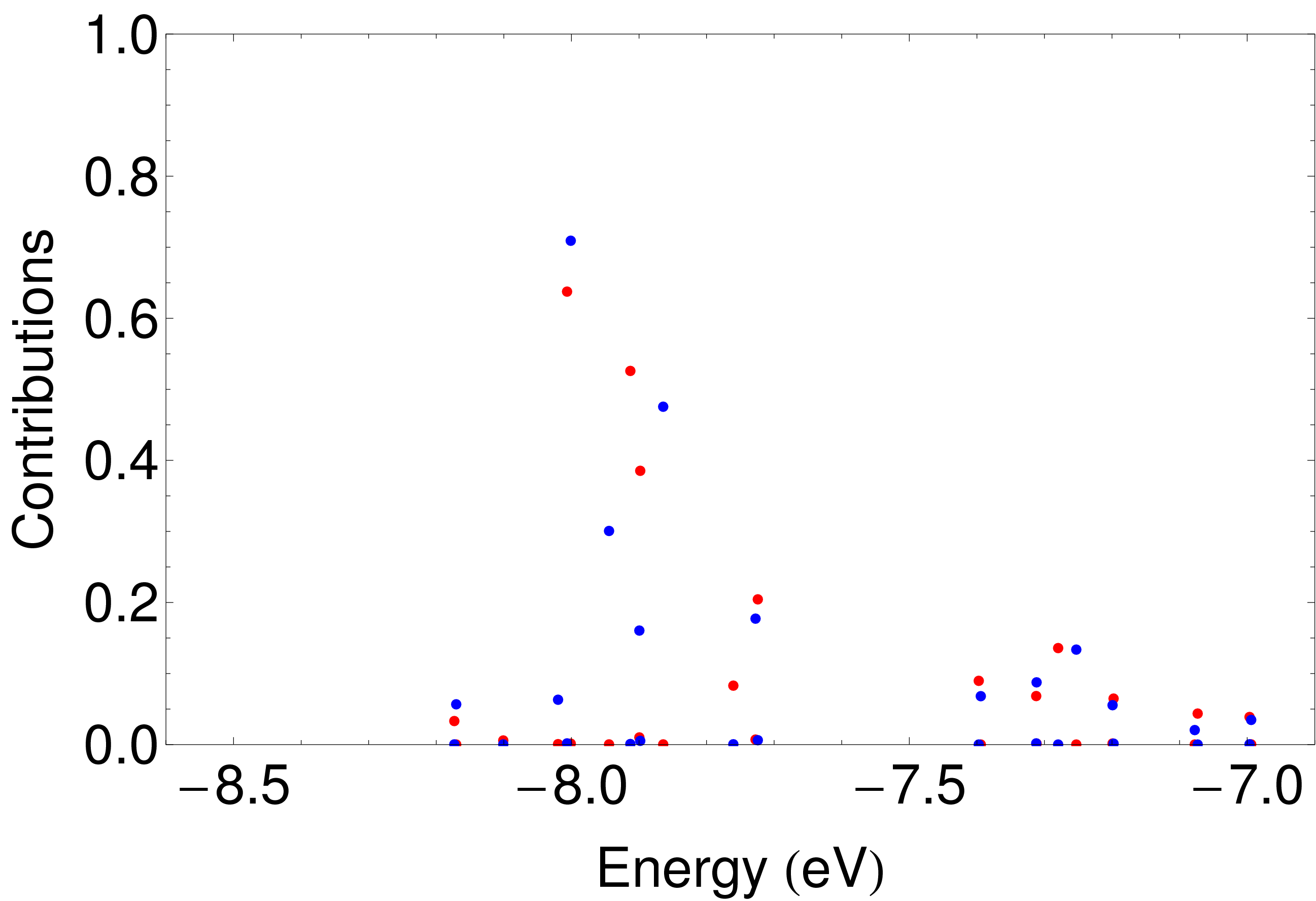
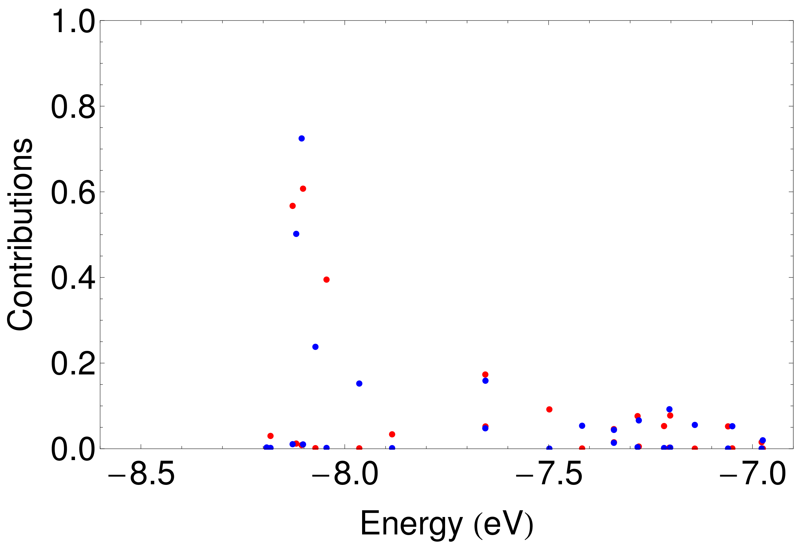
(d)	(e)

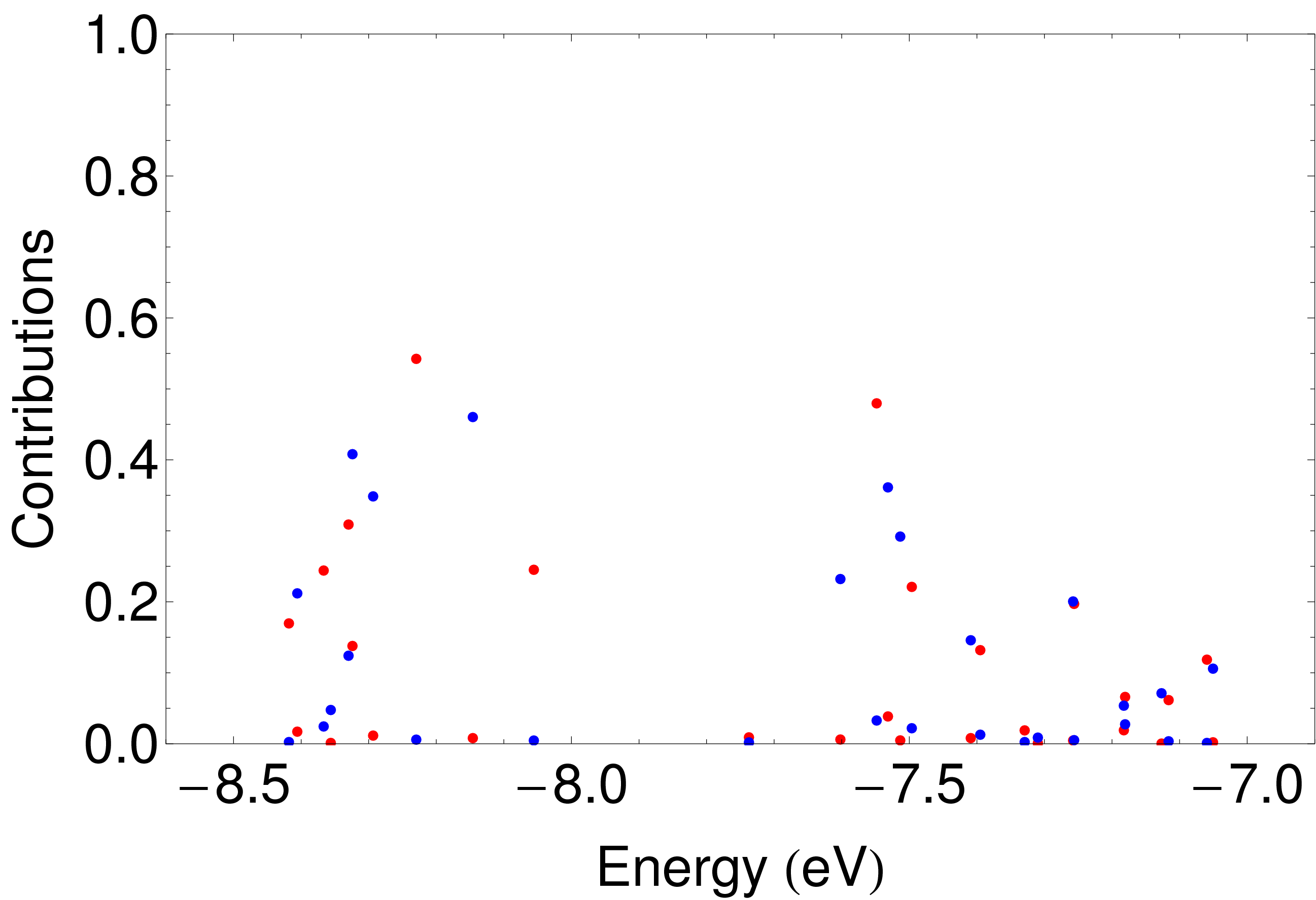
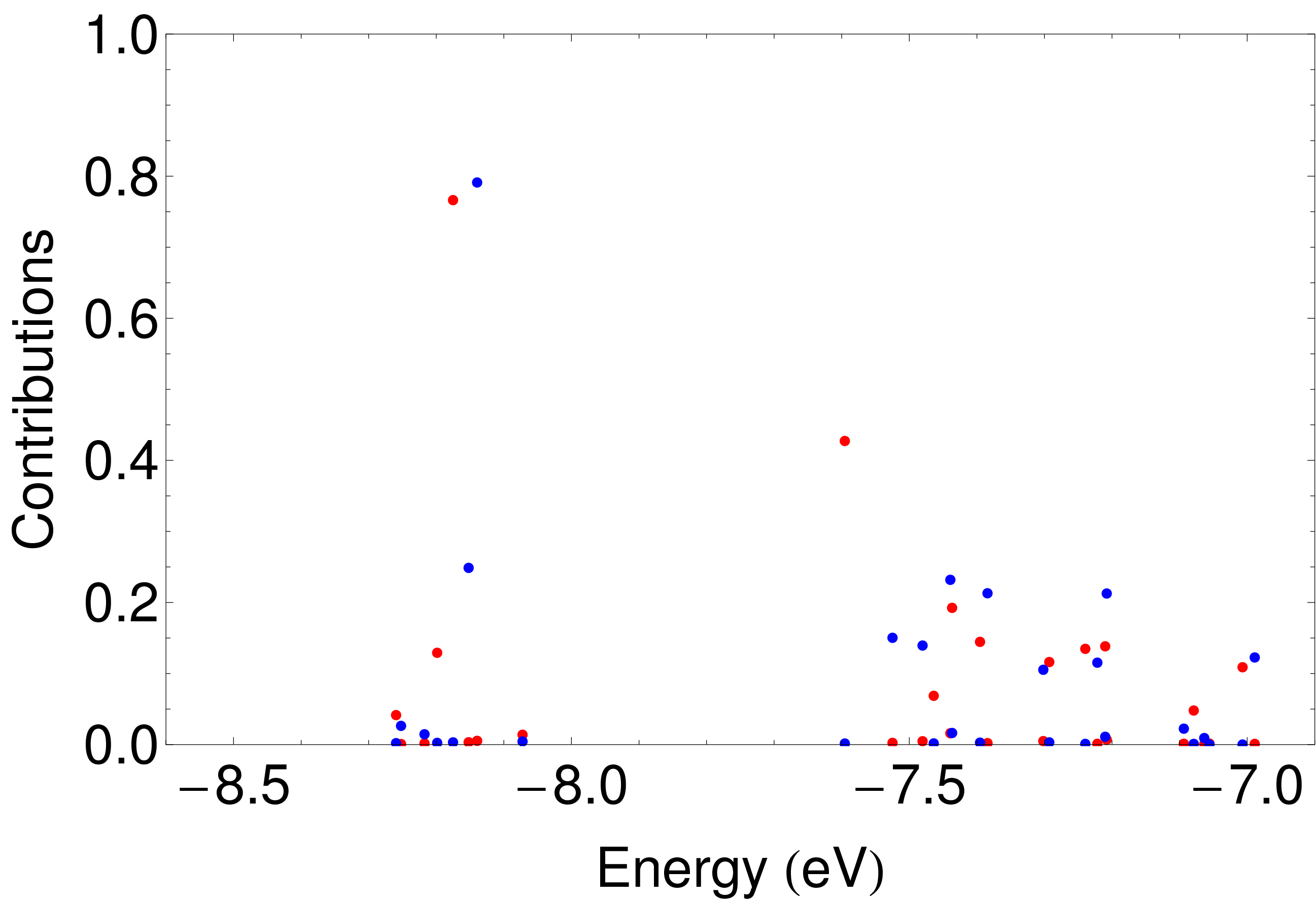
Figure S1: Contributions of the antisymmetric $|C_{a,i}|$ (red) and the symmetric $|C_{s,i}|$ (blue) combinations of the $4f_{xyz}$ orbitals to each Kohn-Sham orbitals for the (a) Gd, (b) Tb, (c) Dy, (d) Ho, (e) Er complexes.

The highest occupied Kohn-Sham orbital for the down spin in the low-symmetry DFT solutions correspond to the $\pi^{*}$ orbital. On the other hand, $4f$ atomic orbitals contribute to many Kohn-Sham orbitals. Thus, the $4f$ orbitals are localized as follows. Because of the inversion symmetry of the complexes, the $4f$ orbital part of each Kohn-Sham orbital $\psi_{i}$ is decomposed into the antisymmetric and symmetric parts:

$$|\psi_{i}\rangle=\frac{1}{\sqrt{2}}\left(|1\rangle+|2\rangle\right)C_{a,i}+\frac{1}{\sqrt{2}}\left(|1\rangle-|2\rangle\right)C_{s,i},$$ (S5)

where, $|1\rangle$ and $|2\rangle$ indicate the $4f_{xyz}$ orbitals on the first and the second lanthanide sites, respectively. The absolute values of $C_{a,i}$ and $C_{s,i}$ for the occupied Kohn-Sham orbitals for the up spin part are shown in Fig. S1. As the antisymmetric and the symmetric levels, we averaged the Kohn-Sham levels:

$$\epsilon_{f,a}=\frac{\sum_{i}^{\text{occ.}}C_{a,i}^{2}\epsilon_{i}}{\sum_{i}^{\text{occ.}}C_{a,i}^{2}},\qquad\epsilon_{f,s}=\frac{\sum_{i}^{\text{occ.}}C_{s,i}^{2}\epsilon_{i}}{\sum_{i}^{\text{occ.}}C_{s,i}^{2}}.$$ (S6)

In Eq. (S6), the sum is taken over occupied Kohn-Sham orbitals. With the use of the levels, the parameters $t$ and $\Delta$ are derived (Table I in the main text). The transfer parameter is gradually decreasing as the increase of the atomic number because the ionic radius of the lanthanide shrinks.

I.2 Calculation of $\pi^{*}\rightarrow 4f$ electron promotion energy for 1

The high- and low-spin states of the complex 1 were analyzed based on the Hubbard Hamiltonian:

$$\hat{H} = \sum_{i=1,2}\sum_{\gamma\sigma}\epsilon_{f}\hat{n}_{i\gamma\sigma}+\sum_{\sigma}\epsilon_{\pi^{*}}\hat{n}_{\pi^{*}\sigma}$$ (S7)

$$+ \sum_{\sigma}t\left(\hat{c}_{1\tilde{\gamma}\sigma}^{\dagger}\hat{c}_{\pi^{*}\sigma}+\hat{c}_{\pi^{*}\sigma}^{\dagger}\hat{c}_{1\tilde{\gamma}\sigma}-\hat{c}_{2\tilde{\gamma}\sigma}^{\dagger}\hat{c}_{\pi^{*}\sigma}-\hat{c}_{\pi^{*}\sigma}^{\dagger}\hat{c}_{2\tilde{\gamma}\sigma}\right)$$

$$+ \sum_{i=1,2}\sum_{\langle\gamma\sigma,\gamma^{\prime}\sigma^{\prime}\rangle}u_{f}\hat{n}_{i\gamma\sigma}\hat{n}_{i\gamma^{\prime}\sigma^{\prime}}+u_{\pi^{*}}\hat{n}_{\pi^{*}\uparrow}\hat{n}_{\pi^{*}\downarrow}$$

$$+ \sum_{i=1,2}\sum_{\gamma\sigma}\sum_{\sigma^{\prime}}v\hat{n}_{\gamma\sigma}\hat{n}_{\pi^{*}\sigma^{\prime}},$$

where $\gamma$ is the component of the $4f$ orbital, $u_{f}$ and $u_{\pi^{*}}$ are the intrasite Coulomb repulsions on Gd and N₂ sites, respectively, and $v$ is the intersite Coulomb repulsion between the Gd and N₂ sites.

The high-spin state with the maximal projection is described by one electron configuration:

$$|1\uparrow,\pi^{*}\uparrow,2\uparrow\rangle,$$ (S8)

where 1 and 2 are the lanthanide sites and $\uparrow$ and $\downarrow$ are spin projections. The $4f$ electrons which are not in the $4f_{xyz}$ orbital are not explicitly written here. The total energy $E_{\rm HS}$ is

$$E_{\rm HS}=E_{0}+(2n+1)\epsilon_{f}+\Delta+2nv+n(n-1)u_{f},$$ (S9)

where $E_{0}$ is the total electronic energy except for the electrons in the $4f$ orbitals and $\pi^{*}$ orbitals, and $n$ is the number of the $4f$ electrons in Gd³⁺ ion. For the low-spin state ($\uparrow,\downarrow,\uparrow$ type), the basis set is

$$\{|1\uparrow,1\downarrow,2\uparrow\rangle,|1\uparrow,\pi^{*}\downarrow,2\uparrow\rangle,|1\uparrow,2\downarrow,2\uparrow\rangle\}.$$ (S10)

Here, the configurations with the electron transfer from the $4f$ to the $\pi^{*}$ are not included because these configurations do not contribute much to the low-energy states due to the large energy gap $\Delta$ between the $4f$ and the $\pi^{*}$ levels. The lowest energy is

$$E_{\rm LS} = E_{0}+(2n+1)\epsilon_{f}+n(n-1)u_{f}$$

$$+ \frac{1}{2}\left(\Delta+2nv+nu_{f}-\sqrt{\left(\Delta+2nv-nu_{f}\right)^{2}+8t^{2}}\right).$$

The energy difference between the low- and high-spin states are

$$\Delta E = E_{\rm LS}-E_{\rm HS}$$

$$= \frac{1}{2}\left[nu_{f}-\left(\Delta+2nv\right)-\sqrt{\left(\Delta+2nv-nu_{f}\right)^{2}+8t^{2}}\right]$$

$$= \frac{1}{2}\left(\bar{U}-\sqrt{\bar{U}^{2}+8t^{2}}\right),$$ (S14)

where

$$\bar{U}=nu_{f}-\Delta-2nv$$ (S15)

is the (averaged) electron promotion energy. Eq. (S15) shows that (i) the energy gap $\Delta$ significantly reduces the promotion energy and (ii) the promotion energy increases with the number of the $4f$ electrons $n$. Using the transfer parameter $t$ derived from the Kohn-Sham orbital, energy gaps between the high-spin state and low-spin state, and Eq. (S14), the averaged promotion energy $\bar{U}$ is derived.

II Ab initio calculations

II.1 Fragment calculations for Ln³⁺ centers in 1-5

To obtain the local electronic properties of the magnetic ions, ab initio quantum chemistry calculations (CASSCF/SO-RASSI) were performed using Molcas Aquilante et al. (2010). In the calculations, one of the metal ions in the complex was replaced by diamagnetic lanthanum ion (La³⁺) and the ligands for the La ion were reduced (Fig. S2). Two point charges ($-0.5$ $e$) were put on each N atom creating the N₂ bridge, where $e$ $(>0)$ is the elementary charge. The latter is to include the electrostatic potential from the unpaired electron of N${}_{2}^{3-}$ bridge. The covalent effect is included later ($\hat{H}^{\prime}_{\text{cf}}$ in the main text). In the CASSCF calculations, all $4f$ orbitals of the magnetic site are included in the active orbitals. The spin-orbit coupling is included in the SO-RASSI calculation. In the SO-RASSI calculations the following CASSCF states were mixed by spin-orbit coupling: for Gd, 1 octet, 48 sextet, 120 quartet and 113 doublet states, for Tb, 7 septet, 140 quintet, 113 triplet and 123 singlet states, for Dy, 21 sextet, 128 quartet and 130 doublet states, for Ho, 35 quintet, 210 triplet and 196 singlet states, and for Er, 35 quartet and 112 doublets states. As the basis set for the calculations, ANO-RCC was used. The contraction of the basis set is shown in Table S1. The Cholesky decomposition threshold was set to $5\times 10^{-8}$ Hartree. The obtained SO-RASSI wave functions were transformed into pseudo spin states (or pseudo $\tilde{J}$ states) Chibotaru and Ungur (2012); Chibotaru (2013); Ungur and Chibotaru (2015); Chibotaru (2015) to analyze the magnetic data using SINGLE_ANISO module ChibotaruSM and Ungur (2006).

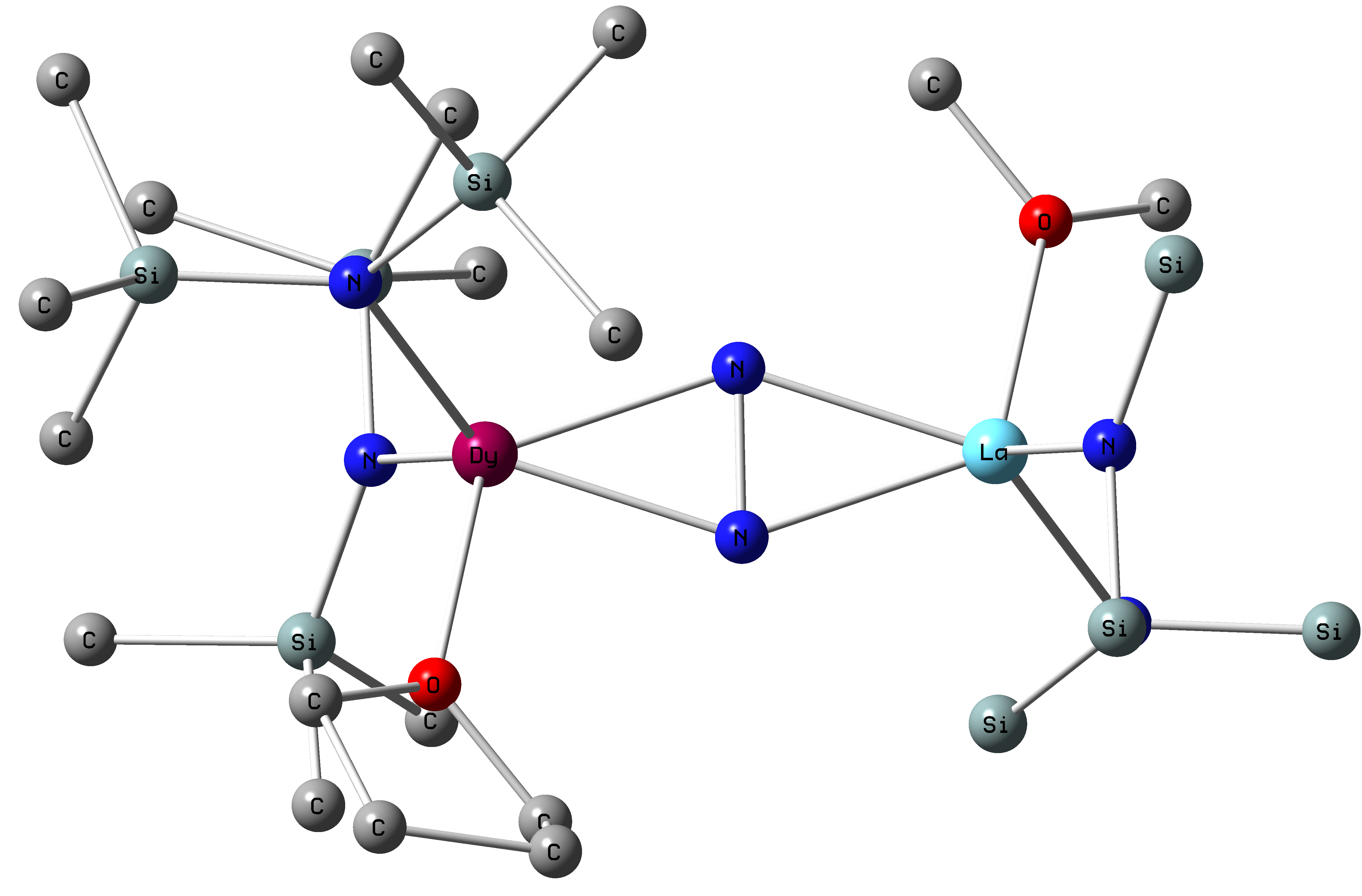
Figure S2: The LnLaN${}_{2}^{3-}$ fragment used in ab initio calculations. Hydrogen atoms are omitted for clarity. The right lanthanide ion was replaced by La in the ab initio calculations.

Table S1: Contractions of the employed ANO-RCC basis sets for the ab initio calculations.

Ln	7s6p4d2f1g	Si	4s3p
La	7s6p4d2f	O	3s2p
N (N2 bridge)	3s2p1d	C	3s2p
N (the others)	3s2p	H	2s

The obtained crystal-field (CF) levels are shown in Table S2. In all cases, the lowest spin-orbit states are doubly degenerate (Kramers doublet for Ln $=$ Gd, Dy, Er) or quasidegenerate (Ising doublet for Ln $=$ Tb, Ho). The ground CF states $|\psi\rangle$ are decomposed into the sum of the ground pseudo $\tilde{J}$ multiplets $|JM\rangle$ Ungur and Chibotaru (2015); Chibotaru (2015):

$$|\psi\rangle=\sum_{M=-J}^{J}C_{M}|JM\rangle.$$ (S16)

The coefficients $C_{M}$ are shown in Table S3. The contributions of the multiplets with the largest projection ($|M|=J$) to the ground CF states are 94.2 %, 96.4 %, 97.1 %, 91.7 %, 78.6 %, for Gd, Tb, Dy, Ho, and Er, respectively. For each ground doublets, the $g$-tensors are calculated (Table S4). The Er complex is not magnetically anisotropic as much as the other complexes (Tb, Dy, Ho). This is because the multiplets $|JM\rangle$ with small $M$ ($|M|<J$) are mixed more than the other systems.

Table S2: The lowest spin-orbit levels of Ln centers obtained by ab initio fragment calculations (cm^-1). The covalency effect is not included.

Gd	Tb	Dy	Ho	Er
0.000	0.000	0.000	0.000	0.000
0.000	0.099	0.000	0.982	0.000
0.329	141.153	179.143	87.999	74.691
0.329	142.222	179.143	88.534	74.691
0.631	288.590	320.747	130.818	118.034
0.631	295.694	320.747	147.454	118.034
1.108	401.446	406.717	167.052	166.279
1.108	435.925	406.717	202.496	166.279
	490.539	470.573	224.559	212.344
	531.201	470.573	241.625	212.344
	547.372	531.942	246.712	262.700
	730.715	531.942	284.704	262.700
	731.087	623.187	296.344	295.345
		623.187	323.988	295.345
		749.919	327.012	396.290
		749.919	385.730	396.290
			386.659

Table S3: $|JM\rangle$ structure of ground CF doublet on Ln³⁺ center in 1-5

Gd		Tb		Dy		Ho		Er
$M$	$|C_{M}|$	$M$	$|C_{M}|$	$M$	$|C_{M}|$	$M$	$|C_{M}|$	$M$	$|C_{M}|$
$-7/2$	0.971	$-6$	0.694	$-15/2$	0.986	$-8$	0.677	$-15/2$	0.887
$-5/2$	0.001	$-5$	0.005	$-13/2$	0.019	$-7$	0.005	$-13/2$	0.112
$-3/2$	0.225	$-4$	0.123	$-11/2$	0.164	$-6$	0.162	$-11/2$	0.321
$-1/2$	0.004	$-3$	0.014	$-9/2$	0.027	$-5$	0.044	$-9/2$	0.168
$1/2$	0.077	$-2$	0.024	$-7/2$	0.023	$-4$	0.084	$-7/2$	0.214
$3/2$	0.002	$-1$	0.008	$-5/2$	0.007	$-3$	0.056	$-5/2$	0.103
$5/2$	0.038	0	0.009	$-3/2$	0.010	$-2$	0.039	$-3/2$	0.105
$7/2$	0.000	1	0.008	$-1/2$	0.004	$-1$	0.033	$-1/2$	0.024
		2	0.024	1/2	0.002	0	0.027	1/2	0.031
		3	0.014	3/2	0.001	1	0.033	3/2	0.021
		4	0.123	5/2	0.001	2	0.039	5/2	0.011
		5	0.005	7/2	0.000	3	0.056	7/2	0.012
		6	0.694	9/2	0.000	4	0.084	9/2	0.016
				11/2	0.000	5	0.044	11/2	0.002
				13/2	0.000	6	0.162	13/2	0.005
				15/2	0.000	7	0.005	15/2	0.000
						8	0.677

Table S4: The $g$ tensors for the lowest doublets of Ln centers obtained from the fragment calculations. The transverse $g$-factors for Tb and Ho are zero because of the Griffith’s theorem Griffith (1963).

	Gd	Tb	Dy	Ho	Er
$g_{X}$	0.492	0.000	0.0026	0.000	0.163
$g_{Y}$	0.824	0.000	0.0040	0.000	0.227
$g_{Z}$	13.439	17.675	19.6459	19.422	16.528

II.2 Calculation of atomic $J$-multiplets of Ln²⁺ ions

The excitation energies of the intermediate virtual electron transferred states were replaced by the excitation energies for isolated Ln²⁺ ion (Ln $=$ Gd, Tb, Dy, Ho, Er). To obtain the energies, the CASSCF and the SO-RASSI calculations were performed with ANO-RCC QZP basis set Aquilante et al. (2010). As in the case of the fragment calculations, all $4f$ orbitals are treated as the active orbitals of the CASSCF calculations. In the SO-RASSI calculations, the following $LS$ terms are included: ${}^{7}F$ for Gd²⁺, ${}^{6}P$, ${}^{6}F$, ${}^{6}H$ for Tb²⁺, ${}^{5}D$, ${}^{5}F$, ${}^{5}G$, ${}^{5}I$ for Dy²⁺, ${}^{4}F$, ${}^{4}G$, ${}^{4}I$ for Ho²⁺, and ${}^{3}F$, ${}^{3}H$ for Er²⁺. The excitation energies $\Delta E$ are shown in Table S5.

Table S5: Excitation energies with respect to the lowest $J$ multiplet of isolated Ln²⁺ ions (meV).

Gd			Tb			Dy
$LS$ term	$J$	$\Delta E$	$LS$ term	$J$	$\Delta E$	$LS$ term	$J$	$\Delta E$
${}^{7}F$	6	0.000	${}^{6}H$	15/2	0.000	${}^{5}I$	8	0.000
	5	182.104		13/2	307.374		7	458.212
	4	333.856		11/2	573.765		6	859.148
	3	455.259		9/2	799.172		5	1202.808
	2	546.311		7/2	983.596		4	1489.190
	1	607.012		5/2	1127.038	${}^{5}G$	6	3412.346
	0	637.362	${}^{6}F$	11/2	1050.937		5	3756.005
				9/2	1276.345		4	4042.388
				7/2	1460.769	${}^{5}F$	5	2369.357
				5/2	1604.210		4	2655.740
			${}^{6}P$	7/2	4357.932	${}^{5}D$	4	5667.150
				5/2	4501.373
Ho			Er
$LS$ term	$J$	$\Delta E$	$LS$ term	$J$	$\Delta E$
${}^{4}I$	15/2	0.000	${}^{3}H$	6	0.000
	13/2	638.260		5	850.945
	11/2	1191.419		4	1197.911
	9/2	1659.477	${}^{3}F$	4	1560.065
${}^{4}G$	11/2	3521.812
	9/2	3989.870
${}^{4}F$	9/2	2461.643

Table S6: Kinetic contributions to the CF parameters $\mathcal{J}_{kq00}$ (cm^-1) for complexes 1-5.

$k$	$q$	$\mathcal{J}_{kq00}$
		Gd	Tb	Dy	Ho	Er
0	0	$-94.88$	$-95.77$	$-70.78$	$-55.38$	$-24.20$
4	0	5.86 $\times 10^{-3}$	$-30.11$	23.76	10.00	$-11.15$
4	$\pm$4	3.50 $\times 10^{-3}$	$-18.00$	14.20	5.97	$-6.66$
6	0	4.12 $\times 10^{-7}$	$-4.95\times 10^{-1}$	6.13	$-8.53$	4.29
6	$\pm$4	$-7.70\times 10^{-7}$	$9.27\times 10^{-1}$	$-11.46$	15.96	$-8.02$

Table S7: Energies of the CF multiplets (cm^-1) of Ln centers in 1-5 originating from the ground atomic $J$-multiplet of the corresponding Ln³⁺ ions, calculated with included kinetic contribution. Due to the latter, the ground CF multiplets of Ln centers are stabilized by 95, 110, 58, 55, 14 cm^-1 for Gd, Tb, Dy, Ho, Er, respectively.

Gd	Tb	Dy	Ho	Er
0.000	0.000	0.000	0.000	0.000
0.000	0.055	0.000	1.297	0.000
0.329	168.191	163.450	95.958	68.276
0.329	168.965	163.450	96.064	68.276
0.630	316.136	300.460	129.220	112.297
0.630	318.418	300.460	147.698	112.297
1.108	426.550	396.451	174.642	150.837
1.108	444.805	396.451	211.117	150.837
	501.172	458.147	223.439	197.730
	541.183	458.147	248.194	197.730
	556.192	510.902	250.839	249.831
	740.636	510.902	280.160	249.831
	741.002	604.121	290.136	276.581
		604.121	320.445	276.581
		747.503	322.767	387.217
		747.503	371.677	387.217
			371.948

Table S8: Energy of the low-lying exchange KDs (cm^-1) in 1-5

Gd	Tb	Dy	Ho	Er
0.000	0.000	0.000	0.000	0.000
0.381	207.619	120.686	105.154	27.999
0.643	207.670	120.686	106.791	28.000
0.865	210.623	158.882	108.718	53.467
1.187	227.323	164.275	110.590	64.209
1.605	362.446	252.462	146.181	68.710
2.112	366.170	273.941	153.019	86.241
27.527	369.751	273.943	160.514	86.254
27.761	369.876	293.589	161.003	99.987

III Analysis of first rank exchange parameters

As shown in Table II in the main text, the first rank part $(k=k^{\prime}=1)$ of the exchange interaction is isotropic Heisenberg type in all complexes, i.e.,

$$\mathcal{J}_{1\pm 11\mp 1}=-\mathcal{J}_{1010}\neq 0,$$ (S17)

and the other $\mathcal{J}_{1q1q^{\prime}}$ are zero. The reason can be understood analyzing the formula of the exchange interaction. The exchange parameter between $J$ multiplet and isotropic spin $1/2$ (Eqs. (2), (3) in the main text) is written as Iwahara and Chibotaru (2015)

$$\mathcal{J}_{kqk^{\prime}q^{\prime}} = \sum_{x}\sum_{\alpha_{J}J}\frac{\left\{t\times t\right\}_{kqk^{\prime}q^{\prime}}^{x}\mathcal{G}^{1}_{\alpha_{J}Jk^{\prime}xk}\tilde{\mathcal{F}}^{2}_{k^{\prime}}}{U_{0}+\Delta E_{\alpha_{J}J}^{n+1}},$$ (S18)

where

$$\{t\times t\}_{kqk^{\prime}q^{\prime}}^{x} = (-1)^{l_{1}-k^{\prime}+q^{\prime}}\sum_{mm^{\prime}}\sum_{\xi}$$ (S19)

$$\times t_{m\pi^{*}}^{12}t_{\pi^{*}m^{\prime}}^{21}C_{l_{1}m^{\prime}kq}^{x\xi}C_{k^{\prime}-q^{\prime}l_{1}m}^{x\xi},$$

$t_{m\pi^{*}}$ is the electron transfer between the $4f$ with component $m$ of orbital angular momentum and the $\pi^{*}$ orbital of N₂, $l_{1}=3$ is the magnitude of the atomic orbital angular momentum for $f$ orbital, $x$ $(l_{1}-k^{\prime}\leq x\leq l_{1}+k^{\prime})$ indicates a rank, $\xi=-x,-x+1,...,x$, $C_{l_{1}m^{\prime}kq}^{x\xi}$ and $C_{k^{\prime}-q^{\prime}l_{1}m}^{x\xi}$ are Clebsch-Gordan coefficients Varshalovich et al. (1988), $\alpha_{J}$ and $J$ are the $LS$-term and the total angular momentum of Ln²⁺, respectively, $\Delta E_{\alpha_{J}J}^{n+1}$ is the excitation multiplet energies of Ln²⁺, and $\mathcal{G}^{\text{Ln}}_{\alpha_{J}Jk^{\prime}xk}$ and $\tilde{\mathcal{F}}^{\text{N}_{2}}_{k^{\prime}}$ are functions of their subscripts. For the detailed description of $x$, $\mathcal{G}^{\text{Ln}}_{\alpha_{J}Jk^{\prime}xk}$, and $\tilde{\mathcal{F}}^{\text{N}_{2}}_{k^{\prime}}$, see Ref. Iwahara and Chibotaru, 2015.

Since the dependence of the exchange parameter (S18) on $q$ and $q^{\prime}$ appears only in $\{t\times t\}_{kqk^{\prime}q^{\prime}}^{x}$ (S19), the condition for the isotropy of $\mathcal{J}_{kq1q^{\prime}}$ is revealed from the equation. First, we consider the cases where only the transfer between $f_{\pm m_{0}}$ orbitals ($m_{0}=0,1,2,3$) and the isotropic spin is nonzero for simplicity. The values of $\{t\times t\}_{1q1q^{\prime}}^{x}$ are tabulated in Table S9. We find that the condition (S17) is fulfilled when $m_{0}=2$, while it is not for other $m_{0}$. In the case of $m_{0}=1$, the nonzero terms with $q=q^{\prime}=\pm 1$ are also the source of the anisotropic exchange. When more than one set of $f$ orbitals $m_{0}$ contribute to the electron transfer, the exchange interaction becomes always anisotropic. Finally, since Eq. (S19) is independent of ions, the condition given above applies to the exchange interaction between any $f$ electron ions and spin $1/2$.

Table S9: $\{t\times t\}_{1q1q^{\prime}}^{x}$ for $m_{0}=0,1,2,3$.

$x$	$q_{1}$	$q_{2}$	$m_{0}$
			0	1	2	3
2	0	0	$\frac{3}{7}|t^{12}_{0\pi^{*}}|^{2}$	$\frac{16}{21}|t^{12}_{1\pi^{*}}|^{2}$	$\frac{10}{21}|t^{12}_{2\pi^{*}}|^{2}$	0
2	$\pm 1$	$\mp 1$	$-\frac{1}{7}|t^{12}_{0\pi^{*}}|^{2}$	$-\frac{1}{3}|t^{12}_{1\pi^{*}}|^{2}$	$-\frac{10}{21}|t^{12}_{2\pi^{*}}|^{2}$	$-\frac{5}{7}|t^{12}_{3\pi^{*}}|^{2}$
2	$\pm 1$	$\pm 1$	0	$-\frac{2}{7}(t^{12}_{\pm 1\pi^{*}})^{2}$	0	0
3	0	0	0	$-\frac{1}{6}|t^{12}_{1\pi^{*}}|^{2}$	$-\frac{2}{3}|t^{12}_{2\pi^{*}}|^{2}$	$-\frac{3}{2}|t^{12}_{3\pi^{*}}|^{2}$
3	$\pm 1$	$\mp 1$	$\frac{1}{2}|t^{12}_{0\pi^{*}}|^{2}$	$\frac{11}{12}|t^{12}_{1\pi^{*}}|^{2}$	$\frac{2}{3}|t^{12}_{2\pi^{*}}|^{2}$	$\frac{1}{4}|t^{12}_{3\pi^{*}}|^{2}$
3	$\pm 1$	$\pm 1$	0	$-\frac{1}{2}(t^{12}_{\pm 1\pi^{*}})^{2}$	0	0
4	0	0	$\frac{4}{7}|t^{12}_{0\pi^{*}}|^{2}$	$\frac{15}{14}|t^{12}_{1\pi^{*}}|^{2}$	$\frac{6}{7}|t^{12}_{2\pi^{*}}|^{2}$	$\frac{1}{2}|t^{12}_{3\pi^{*}}|^{2}$
4	$\pm 1$	$\mp 1$	$-\frac{5}{14}|t^{12}_{0\pi^{*}}|^{2}$	$-\frac{3}{4}|t^{12}_{1\pi^{*}}|^{2}$	$-\frac{6}{7}|t^{12}_{2\pi^{*}}|^{2}$	$-\frac{29}{28}|t^{12}_{3\pi^{*}}|^{2}$
4	$\pm 1$	$\pm 1$	0	$-\frac{3}{14}(t^{12}_{\pm 1\pi^{*}})^{2}$	0	0

References

- Santini et al. (2009) P. Santini, S. Carretta, G. Amoretti, R. Caciuffo, N. Magnani, and G. H. Lander, “Multipolar interactions in -electron systems: The paradigm of actinide dioxides,” Rev. Mod. Phys. 81, 807–863 (2009).
- Zvezdin et al. (1985) A. K. Zvezdin, V. M. Matveev, A. A. Mukhin, and A. I. Popov, Rare Earth Ions in Magnetically Ordered Crystals (Nauka, Moskow, 1985) in Russian.
- Gingras and McClarty (2014) M. J. P. Gingras and P. A. McClarty, “Quantum spin ice: a search for gapless quantum spin liquids in pyrochlore magnets,” Rep. Prog. Phys. 77, 056501 1–26 (2014).
- Gatteschi et al. (2006) D. Gatteschi, R. Sessoli, and J. Villain, Molecular Nanomagnets (Oxford University Press, Oxford, 2006).
- Sessoli et al. (1993) R. Sessoli, D. Gatteschi, A. Caneschi, and M. A. Novak, “Magnetic bistability in a metal-ion cluster,” Nature 365, 141–143 (1993).
- Christou et al. (2000) G. Christou, D. Gatteschi, D. N. Hendrickson, and R. Sessoli, “Single-molecule magnets,” MRS Bulletin 25, 66–71 (2000).
- Coulon et al. (2006) C. Coulon, H. Miyasaka, and R. Clerac, “Single-chain magnets: Theoretical approach and experimental systems,” in Single-Molecule Magnets and Related Phenomena, Struct. Bond., Vol. 122, edited by Winpenny, R (2006) pp. 163–206.
- Heersche et al. (2006) H. B. Heersche, Z. de Groot, J. A. Folk, H. S. J. van der Zant, C. Romeike, M. R. Wegewijs, L. Zobbi, D. Barreca, E. Tondello, and A. Cornia, “Electron transport through single Mn12 molecular magnets,” Phys. Rev. Lett. 96, 206801 (2006).
- Bogani and Wernsdorfer (2008) L. Bogani and W. Wernsdorfer, “Molecular spintronics using single-molecule magnets,” Nat. Mater. 7, 179–186 (2008).
- Leuenberger and Loss (2001) M. N. Leuenberger and D Loss, “Quantum computing in molecular magnets,” Nature 410, 789–793 (2001).
- Timco et al. (2009) G. A. Timco, S. Carretta, F. Troiani, F. Tuna, R. J. Pritchard, C. A. Muryn, E. J. L. McInnes, A. Ghirri, A. Candini, P. Santini, G. Amoretti, M. Affronte, and R. E. P. Winpenny, “Engineering the coupling between molecular spin qubits by coordination chemistry,” Nat. Nanotech. 4, 173–178 (2009).
- Aromi et al. (2012) G. Aromi, D. Aguila, P. Gamez, F. Luis, and O. Roubeau, “Design of magnetic coordination complexes for quantum computing,” Chem. Soc. Rev. 41, 537–546 (2012).
- Ishikawa et al. (2004) N Ishikawa, M Sugita, T Ishikawa, S Koshihara, and Y Kaizu, “Mononuclear lanthanide complexes with a long magnetization relaxation time at high temperatures: A new category of magnets at the single-molecular level,” J. Phys. Chem. B 108, 11265–11271 (2004).
- Rinehart et al. (2011a) J. D. Rinehart, M. Fang, W. J. Evans, and J. R. Long, “Strong exchange and magnetic blocking in N-radical-bridged lanthanide complexes,” Nat. Chem. 3, 538–542 (2011a).
- Woodruff et al. (2013) D. N. Woodruff, R. E. P. Winpenny, and R. A. Layfield, “Lanthanide single-molecule magnets,” Chem. Rev. 113, 5110–5148 (2013).
- Ungur et al. (2014) L. Ungur, S.-Y. Lin, J. Tang, and L. F. Chibotaru, “Single-molecule toroics in Ising-type lanthanide molecular clusters,” Chem. Soc. Rev. 43, 6894–6905 (2014).
- Layfield and Murugesu (2015) R. Layfield and M. Murugesu, eds., Lanthanides and Actinides in Molecular Magnetism (Wiley, New Jersey, 2015).
- Demir et al. (2015) S. Demir, I.-R. Jeon, J. R. Long, and T. D. Harris, “Radical ligand-containing single-molecule magnets,” Coord. Chem. Rev. 289,290, 149–176 (2015).
- Dieke (1967) G. H. Dieke, Spectra and Energy Levels of Rare-Earth Ions in Crystals (Academic Press Inc., New York, 1967).
- Ungur and Chibotaru (2011) L. Ungur and L. F. Chibotaru, “Magnetic anisotropy in the excited states of low symmetry lanthanide complexes,” Phys. Chem. Chem. Phys. 13, 20086–20090 (2011).
- Chibotaru (2015) L. F. Chibotaru, “Theoretical understanding of Anisotropy in Molecular Nanomagnets,” in Molecular Nanomagnets and Related Phenomena, Struct. Bond., Vol. 164, edited by Song Gao (Springer Berlin Heidelberg, 2015) pp. 185–229.
- Chibotaru et al. (2008) L. F Chibotaru, L. Ungur, and A. Soncini, “The origin of nonmagnetic Kramers doublets in the ground state of dysprosium triangles: evidence for a toroidal magnetic moment,” Angew. Chem. Int. Ed. 120, 4194–4197 (2008).
- Chibotaru and Iwahara (2015) L. F. Chibotaru and N. Iwahara, “Ising exchange interaction in lanthanides and actinides,” New J. Phys. 17, 103028 1–15 (2015).
- Rinehart et al. (2011b) J. D. Rinehart, M. Fang, W. J. Evans, and J. R. Long, “A N-Radical-Bridged terbium complex exhibiting magnetic hysteresis at 14 K,” J. Am. Chem. Soc. 133, 14236–14239 (2011b).
- Chibotaru and Ungur (2012) L. F. Chibotaru and L. Ungur, “Ab initio calculation of anisotropic magnetic properties of complexes. I. Unique definition of pseudospin Hamiltonians and their derivation,” J. Chem. Phys. 137, 064112 1–22 (2012).
- Ungur and Chibotaru (2015) L. Ungur and L. F. Chibotaru, “Computational Modelling of the Magnetic Properties of Lanthanide Compounds,” in Lanthanides and Actinides in Molecular Magnetism, edited by R. Layfield and M. Murugesu (Wiley, New Jersey, 2015) pp. 153–184.
- Soda et al. (2000) T. Soda, Y. Kitagawa, T. Onishi, Y. Takano, Y. Shigeta, H. Nagao, Y. Yoshioka, and K. Yamaguchi, “Ab initio computations of effective exchange integrals for H-–H, H–-He-–H and Mn2O2 complex: comparison of broken-symmetry approaches,” Chem. Phys. Lett. 319, 223–230 (2000).
- Rajeshkumar and Rajaraman (2012) T. Rajeshkumar and G. Rajaraman, “Is a radical bridge a route to strong exchange interactions in lanthanide complexes? A computational examination,” Chem. Commun. 48, 7856–7858 (2012).
- Zhang et al. (2013) Y.-Q. Zhang, C.-L. Luo, B.-W. Wang, and S. Gao, “Understanding the Magnetic Anisotropy in a Family of N Radical-Bridged Lanthanide Complexes: Density Functional Theory and ab Initio Calculations,” J. Phys. Chem. A 117, 10873–10880 (2013).
- van der Marel and Sawatzky (1988) D. van der Marel and G. A. Sawatzky, “Electron-electron interaction and localization in and transition metals,” Phys. Rev. B 37, 10674–10684 (1988).
- Anderson (1959) P. W. Anderson, “New approach to the theory of superexchange interactions,” Phys. Rev. 115, 2–13 (1959).
- Anderson (1963) P. W. Anderson, “Theory of magnetic exchange interactions: exchange in insulators and semiconductors,” in Solid State Physics, Vol. 14, edited by F. Seitz and D. Turnbull (Academic Press, New York, 1963) pp. 99–214.
- Goodenough (1963) J. B. Goodenough, Magnetism and the Chemical Bond (John Wiley & Sons, New York, 1963).
- Iwahara and Chibotaru (2015) N. Iwahara and L. F. Chibotaru, “Exchange interaction between multiplets,” Phys. Rev. B 91, 174438 1–18 (2015).
- Stevens (1952) K. W. H. Stevens, “Matrix Elements and Operator Equivalents Connected with the Magnetic Properties of Rare Earth Ions,” Proc. Phys. Soc. London, Sec. A 65, 209–215 (1952).
- Moriya (1960) T. Moriya, “Anisotropic Superexchange Interaction and weak Ferromagnetism,” Phys. Rev. 120, 91–98 (1960).
- Elliott and Thorpe (1968) R. J. Elliott and M. F. Thorpe, “Orbital effects on exchange interactions,” J. Appl. Phys. 39, 802–807 (1968).
- Hartmann-Boutron (1968) F. Hartmann-Boutron, “Interactions de superéchange en présence de dégénérescence orbitale et de couplage spin-orbite,” J. Phys. France 29, 212–214 (1968).
- Imada and Miyake (2010) M. Imada and T. Miyake, “Electronic structure calculation by first principles for strongly correlated electron systems,” J. Phys. Soc. Jpn. 79, 112001 1–42 (2010).
- Solovyev (2008) I. V. Solovyev, “Combining dft and many-body methods to understand correlated materials,” J. Phys.: Condens. Matter 20, 293201 1–33 (2008).
- Neese (2012) F. Neese, “The ORCA program system,” WIREs Comput. Mol. Sci. 2, 73–78 (2012).
- Polo et al. (2003) V. Polo, J. Gräfenstein, E. Kraka, and D. Cremer, “Long-range and short-range Coulomb correlation effects as simulated by Hartree–-Fock, local density approximation, and generalized gradient approximation exchange functionals,” Theor. Chem. Acc. 109, 22–35 (2003).
- Ruiz et al. (2005) E. Ruiz, S. Alvarez, J. Cano, and V. Polo, “About the calculation of exchange coupling constants using density-functional theory: The role of the self-interaction error,” J. Chem. Phys. 123, 164110 1–7 (2005).
- Aquilante et al. (2010) F. Aquilante, L. De Vico, N. Ferré, G. Ghigo, P.-å. Malmqvist, P. Neogrády, T. B. Pedersen, M. Pitoňák, M. Reiher, B. Roos, et al., “Molcas 7: The next generation,” J. Comput. Chem. 31, 224–247 (2010).
- Chibotaru and Ungur (2006) L. F. Chibotaru and L. Ungur, “The computer programs SINGLE_ANISO and POLY_ANISO,” University of Leuven (2006).
Supplemental Materials
for

References

- Aquilante et al. (2010) F. Aquilante, L. De Vico, N. Ferré, G. Ghigo, P.-å. Malmqvist, P. Neogrády, T. B. Pedersen, M. Pitoňák, M. Reiher, B. Roos, et al., “Molcas 7: The next generation,” J. Comput. Chem. 31, 224–247 (2010).
- Chibotaru and Ungur (2012) L. F. Chibotaru and L. Ungur, “Ab initio calculation of anisotropic magnetic properties of complexes. I. Unique definition of pseudospin Hamiltonians and their derivation,” J. Chem. Phys. 137, 064112 1–22 (2012).
- Chibotaru (2013) L. F. Chibotaru, “Ab initio methodology for pseudospin Hamiltonians of anisotropic magnetic complexes,” in Adv. Chem. Phys., Vol. 153, edited by S. A. Rice and A. R. Dinner (Johns Wiley & Sons, New Jersey, 2013) pp. 397–519.
- Ungur and Chibotaru (2015) L. Ungur and L. F. Chibotaru, “Computational Modelling of the Magnetic Properties of Lanthanide Compounds,” in Lanthanides and Actinides in Molecular Magnetism, edited by R. Layfield and M. Murugesu (Wiley, New Jersey, 2015) Chap. 6.
- Chibotaru (2015) L. F. Chibotaru, “Theoretical understanding of Anisotropy in Molecular Nanomagnets,” in Molecular Nanomagnets and Related Phenomena, Struct. Bond., Vol. 164, edited by Song Gao (Springer Berlin Heidelberg, 2015) pp. 185–229.
- ChibotaruSM and Ungur (2006) L. F. Chibotaru and L. Ungur, “The computer programs SINGLE_ANISO and POLY_ANISO,” University of Leuven (2006).
- Griffith (1963) J. S. Griffith, “Spin Hamiltonian for even-electron systems having even multiplicity,” Phys. Rev. 132, 316–319 (1963).
- Iwahara and Chibotaru (2015) N. Iwahara and L. F. Chibotaru, “Exchange interaction between multiplets,” Phys. Rev. B 91, 174438 1–18 (2015).
- Varshalovich et al. (1988) D. A. Varshalovich, A. N. Moskalev, and V. K. Khersonskii, Quantum Theory of Angular Momentum (World Scientific, Singapore, 1988).