Annealed scaling for a charged polymer

Abstract.

This paper studies an undirected polymer chain living on the one-dimensional integer lattice and carrying i.i.d. random charges. Each self-intersection of the polymer chain contributes to the interaction Hamiltonian an energy that is equal to the product of the charges of the two monomers that meet. The joint probability distribution for the polymer chain and the charges is given by the Gibbs distribution associated with the interaction Hamiltonian. The focus is on the annealed free energy per monomer in the limit as the length of the polymer chain tends to infinity.

We derive a spectral representation for the free energy and use this to prove that there is a critical curve in the parameter plane of charge bias versus inverse temperature separating a ballistic phase from a subballistic phase. We show that the phase transition is first order. We prove large deviation principles for the laws of the empirical speed and the empirical charge, and derive a spectral representation for the associated rate functions. Interestingly, in both phases both rate functions exhibit flat pieces, which correspond to an inhomogeneous strategy for the polymer to realise a large deviation. The large deviation principles in turn lead to laws of large numbers and central limit theorems. We identify the scaling behaviour of the critical curve for small and for large charge bias. In addition, we identify the scaling behaviour of the free energy for small charge bias and small inverse temperature. Both are linked to an associated Sturm-Liouville eigenvalue problem.

A key tool in our analysis is the Ray-Knight formula for the local times of the one-dimensional simple random walk. This formula is exploited to derive a closed form expression for the generating function of the annealed partition function, and for several related quantities. This expression in turn serves as the starting point for the derivation of the spectral representation for the free energy, and for the scaling theorems.

What happens for the quenched free energy per monomer remains open. We state two modest results and raise a few questions.

1. Introduction

1.1. Motivation

DNA and proteins are polyelectrolytes whose monomers are in a charged state that depends on the pH of the solution in which they are immersed. The charges may fluctuate in space (‘quenched’) and in time (‘annealed’).

In this paper we consider the charged polymer chain introduced in Kantor and Kardar [30]. The polymer chain is modelled by the path of a simple random walk on $\mathbb{Z}^{d}$, $d\geq 1$. Each monomer in the polymer chain carries a random electric charge, drawn in an i.i.d. fashion from $\mathbb{R}$. Each self-intersection of the polymer chain contributes an energy that is equal to the product of the charges of the two monomers that meet (i.e., a negative energy when the charges have opposite sign and a positive energy when the charges have the same sign). The polymer chain has a probability distribution on path space that is given by the Gibbs measure associated with the energy. Our goal is to study the scaling properties of the polymer as its length tends to infinity.

Very little is known mathematically about the quenched version of the model, where the charges are frozen. The two main questions of interest are:

• Is the free energy self-averaging in the disorder?

• Is there a phase transition from a ‘collapsed phase’ to an ‘extended phase’ at some critical value of the temperature?

We expect that the answer to (1) is yes and the answer to (2) is no. All we are able to show is the following (see Appendix B):

• If the average charge is non-zero, then the number of different sites visited by the polymer is proportional to its length.

• In $d=1$, if the average charge is sufficiently positive or negative and the temperature is sufficiently low, then the polymer behaves ballistically.

We expect that in any $d\geq 1$ the scaling of the polymer is similar to that of the self-avoiding walk when the average charge is non-zero. We further expect that the polymer is subdiffusive when the average charge is zero. All these problems remains open.

In the present paper we focus on the annealed version of the model, where the charges are averaged out. This version, which we study in $d=1$ only, is easier to deal with, yet turns out to exhibit a very rich scaling behavior. The answer to (2) is yes for the annealed model. We will obtain a detailed description of the phase transition curve separating a subballistic phase from a ballistic phase. Moreover, we show that the phase transition is first order, and show that the empirical speed and the empirical charge satisfy a law of large numbers, a central limit theorem, as well as a large deviation principle with a rate function that exhibits flat pieces. The latter corresponds to an inhomogeneous strategy for the polymer to realise a large deviation. We identify the scaling of the free energy in the limit of small average charge and small inverse temperature, which exhibits anomalous behaviour.

A key tool in our analysis is the Ray-Knight formula for the local times of the one-dimensional simple random walk. This tool, which has been used extensively in the literature, is exploited in full throughout the paper in order to obtain the fine details of the phase diagram of the charged polymer. The Ray-Knight formula is no longer available in $d\geq 2$. In Berger, den Hollander and Poisat [5] it is shown that the phase diagram is qualitatively similar, but no detailed description of the scaling behaviour in the two phases is obtained.

The outline of the paper is as follows. In Section 1.2 we define the model. In Section 1.3 we state six theorems with general properties and in Section 1.4 three theorems with asymptotic properties. In Section 1.5 we discuss these theorems. Proofs are given in Sections 2–4. Appendices A–C contain a few technical computations, while Appendix D states two modest results for the quenched version of the model.

1.2. Model and assumptions

Throughout the paper we use the notation $\mathbb{N}=\{1,2,\dots\}$ and $\mathbb{N}_{0}=\mathbb{N}\cup\{0\}$.

Let $S=(S_{i})_{i\in\mathbb{N}_{0}}$ be a simple random walk on $\mathbb{Z}^{d}$, $d\geq 1$, i.e., $S_{0}=0$ and $S_{i}=\sum_{j=1}^{i}X_{j}$, $i\in\mathbb{N}$, with $X=(X_{j})_{j\in\mathbb{N}}$ i.i.d. random variables such that $\mathrm{P}(X_{1}=x)=\tfrac{1}{2d}$ for $x\in\mathbb{Z}^{d}$ with $\|x\|=1$ and zero otherwise ($\|\cdot\|$ denotes the lattice norm). The path $S$ models the configuration of the polymer chain, i.e., $S_{i}$ is the location of monomer $i$. We use the letters $\mathrm{P}$ and $\mathrm{E}$ for probability and expectation with respect to $S$.

Let $\omega=(\omega_{i})_{i\in\mathbb{N}}$ be i.i.d. random variables taking values in $\mathbb{R}$. The sequence $\omega$ models the electric charges along the polymer chain, i.e., $\omega_{i}$ is the charge of monomer $i$ (see Fig. 1). We use the letters ${\mathbb{P}}$ and ${\mathbb{E}}$ for probability and expectation with respect to $\omega$. Throughout the paper we assume that

(1.1) $$M(t)={\mathbb{E}}(e^{t\omega_{1}})<\infty\qquad\forall\,t\in\mathbb{R}.$$

Without loss of generality we may take (see (1.6)–(1.8) below)

(1.2) $${\mathbb{E}}(\omega_{1})=0,\qquad{\mathbb{V}\mathrm{ar}}(\omega_{1})=1.$$

To allow for biased charges, we use a tilting parameter $\delta\in\mathbb{R}$ and write ${\mathbb{P}}^{\delta}$ for the i.i.d. law of $\omega$ with marginal

(1.3) $${\mathbb{P}}^{\delta}(\text{\rm d}\omega_{1})=\frac{e^{\delta\omega_{1}}\,{\mathbb{P}}(\text{\rm d}\omega_{1})}{M(\delta)}.$$

Note that ${\mathbb{E}}^{\delta}(\omega_{1})=M^{\prime}(\delta)/M(\delta)$. In what follows we may, without loss of generality, take $\delta\in[0,\infty)$.

Example: The special case where the charges are $+1$ with probability $p$ and $-1$ with probability $1-p$ for some $p\in(0,1)$ corresponds to ${\mathbb{P}}=[\tfrac{1}{2}(\delta_{-1}+\delta_{+1})]^{\otimes\mathbb{N}}$ and $\delta=\tfrac{1}{2}\log(\frac{p}{1-p})$.

Let $\Pi$ denote the set of nearest-neighbor paths starting at $0$. Given $n\in\mathbb{N}$, we associate with each $(\omega,S)\in\mathbb{R}^{\mathbb{N}}\times\Pi$ an energy given by the Hamiltonian (see Fig. 1)

(1.4) $$H_{n}^{\omega}(S)=\sum_{1\leq i<j\leq n}\omega_{i}\omega_{j}\,{\sf 1}_{\{S_{i}=S_{j}\}}.$$

Let $\beta$ denote the inverse temperature. Throughout the sequel the relevant space for the pair of parameters $(\delta,\beta)$ is the quadrant

(1.5) $${\mathcal{Q}}=[0,\infty)\times(0,\infty).$$

Given $(\delta,\beta)\in{\mathcal{Q}}$, the annealed polymer measure of length $n$ is the Gibbs measure ${\mathbb{P}}_{n}^{\delta,\beta}$ defined as

(1.6) $$\frac{\text{\rm d}{\mathbb{P}}_{n}^{\delta,\beta}}{\text{\rm d}({\mathbb{P}}^{\delta}\times\mathrm{P})}(\omega,S)=\frac{1}{{\mathbb{Z}}_{n}^{\delta,\beta}}\,e^{-\beta H_{n}^{\omega}(S)},\qquad(\omega,S)\in\mathbb{R}^{\mathbb{N}}\times\Pi,$$

where

(1.7) $$\mathbb{Z}_{n}^{\delta,\beta}=({\mathbb{E}}^{\delta}\times\mathrm{E})\left[e^{-\beta H_{n}^{\omega}(S)}\right]$$

is the annealed partition function of length $n$. The measure ${\mathbb{P}}_{n}^{\delta,\beta}$ is the joint probability distribution for the polymer chain and the charges at charge bias $\delta$ and inverse temperature $\beta$ when the polymer chain has length $n$.

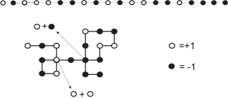
Figure 1. Top: A polymer chain carrying $(\pm 1)$-valued random charges. Bottom: The path may or may not be self-avoiding. The charges only interact at self-intersections.

In what follows, instead of (1.4) we will work with the Hamiltonian

(1.8) $$H_{n}^{\omega}(S)=\sum_{1\leq i,j\leq n}\omega_{i}\omega_{j}\,{\sf 1}_{\{S_{i}=S_{j}\}}=\sum_{x\in\mathbb{Z}^{d}}\left(\sum_{i=1}^{n}\omega_{i}\,{\sf 1}_{\{S_{i}=x\}}\right)^{2}.$$

The sum under the square is the local time of $S$ at site $x$ weighted by the charges that are encountered in $\omega$. The change from (1.4) to (1.8) amounts to replacing $\beta$ by $2\beta$ and adding a charge bias (see Section 2.2 for more details).

1.3. Theorems: general properties

Let $Q(i,j)$ be the probability matrix defined by

(1.9) $$Q(i,j)=\begin{cases}{\sf 1}_{\{j=0\}},&\text{if }i=0,\ j\in\mathbb{N}_{0},\\ \rule{0.0pt}{20.00003pt}\displaystyle\binom{i+j-1}{i-1}\left(\frac{1}{2}\right)^{i+j},&\text{if }i\in\mathbb{N},\ j\in\mathbb{N}_{0},\end{cases}$$

which is the transition kernel of a critical Galton-Watson branching process with a geometric offspring distribution (of parameter $\frac{1}{2}$). For $(\delta,\beta)\in{\mathcal{Q}}$, let $G^{*}_{\delta,\beta}$ be the function defined by

(1.10) $$G^{*}_{\delta,\beta}(\ell)=\log{\mathbb{E}}\left[e^{\delta\Omega_{\ell}-\beta\Omega_{\ell}^{2}}\right]\quad\text{ with}\quad\Omega_{\ell}=\sum_{k=1}^{\ell}\omega_{k},\qquad\ell\in\mathbb{N}_{0}.$$

($\Omega_{0}=0$.) For $(\mu,\delta,\beta)\in[0,\infty)\times{\mathcal{Q}}$, define the $\mathbb{N}_{0}\times\mathbb{N}_{0}$ matrices ${A}_{\mu,\delta,\beta}$ and $\widetilde{A}_{\mu,\delta,\beta}$ by

(1.11) $$A_{\mu,\delta,\beta}(i,j) =e^{-\mu(i+j+1)+G^{*}_{\delta,\beta}(i+j+1)}\,Q(i+1,j),\qquad i,j\in\mathbb{N}_{0},$$

(1.12) $$\widetilde{A}_{\mu,\delta,\beta}(i,j) =\begin{cases}0,&\text{ if }i=0,\,j\in\mathbb{N}_{0},\\ A_{\mu,\delta,\beta}(i-1,j),&\text{ if }i\in\mathbb{N},\,j\in\mathbb{N}_{0}.\end{cases}$$

Note that ${A}_{\mu,\delta,\beta}$ is symmetric while $\widetilde{A}_{\mu,\delta,\beta}$ is not.

Let $\lambda_{\delta,\beta}(\mu)$ and $\widetilde{\lambda}_{\delta,\beta}(\mu)$ be the spectral radius of $A_{\mu,\delta,\beta}$, respectively, $\widetilde{A}_{\mu,\delta,\beta}$ in $\ell^{2}(\mathbb{N}_{0})$. We will see in Section 2.4 that, for every $(\delta,\beta)\in{\mathcal{Q}}$, both $\mu\mapsto\lambda_{\delta,\beta}(\mu)$ and $\mu\mapsto\widetilde{\lambda}_{\delta,\beta}(\mu)$ are continuous, strictly decreasing and log-convex on $[0,\infty)$, tend to zero at infinity, and satisfy $\widetilde{\lambda}_{\delta,\beta}(\mu)<\lambda_{\delta,\beta}(\mu)$ for all $\mu\in[0,\infty)$. Let

(1.13) $$\begin{array}[]{ll}&\bullet\,\,\mu(\delta,\beta)\text{ be the unique solution of the equation }\lambda_{\delta,\beta}(\mu)=1\\ &\text{when it exists and }\mu(\delta,\beta)=0\text{ otherwise},\\ &\bullet\,\,\widetilde{\mu}(\delta,\beta)\text{ be the unique solution of the equation }\widetilde{\lambda}_{\delta,\beta}(\mu)=1\\ &\text{when it exists and }\widetilde{\mu}(\delta,\beta)=0\text{ otherwise},\end{array}$$

which satisfy $\widetilde{\mu}(\delta,\beta)\leq\mu(\delta,\beta)$, with strict inequality as soon as $\mu(\delta,\beta)>0$. We will also see that, for every $(\delta,\beta)\in{\mathcal{Q}}$, $\mu\mapsto\lambda_{\delta,\beta}(\mu)$ is analytic and strictly log-convex on $(0,\infty)$, and has a finite strictly negative right-slope at $0$ (see Fig. 2).

Figure 2. Qualitative plot of $\mu\mapsto\log\lambda_{\delta,\beta}(\mu)$ (top curve) and $\mu\mapsto\log\widetilde{\lambda}_{\delta,\beta}(\mu)$ (bottom curve) for fixed $(\delta,\beta)\in{\mathcal{Q}}$. Only the case $\lambda_{\delta,\beta}(0)>\widetilde{\lambda}_{\delta,\beta}(0)>1$ is shown. The interior of the ballistic phase ${\rm int}({\mathcal{B}})$ corresponds to $\lambda_{\delta,\beta}(0)>1$, the subballistic phase ${\mathcal{S}}$ corresponds to $\lambda_{\delta,\beta}(0)<1$, the critical curve corresponds to $\lambda_{\delta,\beta}(0)=1$ (see (1.21)).

We begin with a spectral representation for the annealed free energy. Abbreviate

(1.14) $$f(\delta)=-\log M(\delta)\in(-\infty,0].$$

Theorem 1.1.

For all $(\delta,\beta)\in{\mathcal{Q}}$, the annealed free energy per monomer

(1.15) $$F(\delta,\beta)=\lim_{n\to\infty}\frac{1}{n}\,\log{\mathbb{Z}}_{n}^{\delta,\beta}$$

exists, takes values in $(-\infty,0]$, and satisfies the inequality

(1.16) $$F(\delta,\beta)\geq f(\delta).$$

Moreover, the excess free energy

(1.17) $$F^{*}(\delta,\beta)=F(\delta,\beta)-f(\delta)$$

is convex in $(\delta,\beta)$ and has the spectral representation

(1.18) $$F^{*}(\delta,\beta)=\mu(\delta,\beta).$$

The inequality in (1.16) leads us to define two phases:

(1.19) $${\mathcal{Q}}^{>} =\big{\{}(\delta,\beta)\in{\mathcal{Q}}\colon\,F^{*}(\delta,\beta)>0\big{\}},$$

$${\mathcal{Q}}^{=} =\{(\delta,\beta)\in{\mathcal{Q}}\colon\,F^{*}(\delta,\beta)=0\big{\}}.$$

We next show that these phases are separated by a single critical curve (see Fig. 3) and that there are no further subphases.

Figure 3. Qualitative plot of the critical curve $\delta\mapsto\beta_{c}(\delta)$ where the excess free energy $F^{*}(\delta,\beta)$ changes from being zero to being strictly positive (see (1.19)). The critical curve is part of ${\mathcal{Q}}^{=}$.

Theorem 1.2.

There exists a critical curve $\delta\mapsto\beta_{c}(\delta)$ such that

(1.20) $${\mathcal{Q}}^{>} =\big{\{}(\delta,\beta)\in{\mathcal{Q}}\colon\,0<\beta<\beta_{c}(\delta)\big{\}},$$

$${\mathcal{Q}}^{=} =\big{\{}(\delta,\beta)\in{\mathcal{Q}}\colon\,\beta\geq\beta_{c}(\delta)\big{\}}.$$

For every $\delta\in[0,\infty)$, $\beta_{c}(\delta)$ is the unique solution of the equation $\lambda_{\delta,\beta}(0)=1$. Moreover, $\delta\mapsto\beta_{c}(\delta)$ is continuous, strictly increasing and convex on $[0,\infty)$, analytic on $(0,\infty)$, and satisfies $\beta_{c}(0)=0$. In addition, $(\delta,\beta)\mapsto F^{*}(\delta,\beta)$ is analytic on ${\mathcal{Q}}^{>}$.

Let

(1.21) $${\mathcal{B}}=\big{\{}(\delta,\beta)\in{\mathcal{Q}}\colon\,0<\beta\leq\beta_{c}(\delta)\big{\}},\qquad{\mathcal{S}}={\mathcal{Q}}\backslash{\mathcal{B}}.$$

The set ${\mathcal{B}}$ will be referred to as the ballistic phase, the set ${\mathcal{S}}$ as the subballistic phase, for reasons we explain next. Namely, we proceed by stating a law of large numbers for the empirical speed $n^{-1}S_{n}$ and the empirical charge $n^{-1}\Omega_{n}$, respectively, with

(1.22) $$S_{n}=\sum_{i=1}^{n}X_{i},\qquad\Omega_{n}=\sum_{i=1}^{n}\omega_{i}.$$

In the statement below the condition $S_{n}>0$ is put in to choose a direction for the endpoint of the polymer chain.

Theorem 1.3.

For every $(\delta,\beta)\in{\mathcal{Q}}$ there exists a $v(\delta,\beta)\in[0,1]$ such that

(1.23) $$\lim_{n\to\infty}{\mathbb{P}}_{n}^{\delta,\beta}\Big{(}\big{|}n^{-1}S_{n}-v(\delta,\beta)\big{|}>\varepsilon\,\Big{|}\,S_{n}>0\Big{)}=0\qquad\forall\,\varepsilon>0,$$

where

(1.24) $$v(\delta,\beta)\left\{\begin{array}[]{ll}>0,&(\delta,\beta)\in{\mathcal{B}},\\ =0,&(\delta,\beta)\in{\mathcal{S}}.\end{array}\right.$$

For every $(\delta,\beta)\in{\mathcal{B}}$,

(1.25) $$\frac{1}{v(\delta,\beta)}=\left[-\frac{\partial}{\partial\mu}\log\lambda_{\delta,\beta}(\mu)\right]_{\mu=\mu(\delta,\beta)}=\left[-\frac{\partial}{\partial\mu}\lambda_{\delta,\beta}(\mu)\right]_{\mu=\mu(\delta,\beta)}.$$

(Take the right-derivative when $\mu(\delta,\beta)=0$; see Fig. 2.) Moreover, $(\delta,\beta)\mapsto v(\delta,\beta)$ is analytic on ${\rm int}({\mathcal{B}})$.

Theorem 1.4.

For every $(\delta,\beta)\in{\mathcal{Q}}$, there exists a $\rho(\delta,\beta)\in[0,\infty)$ such that

(1.26) $$\lim_{n\to\infty}{\mathbb{P}}_{n}^{\delta,\beta}\left(\left|n^{-1}\Omega_{n}-\rho(\delta,\beta)\right|>\varepsilon\right)=0\qquad\forall\,\varepsilon>0,$$

where

(1.27) $$\rho(\delta,\beta)\left\{\begin{array}[]{ll}>0,&(\delta,\beta)\in{\mathcal{B}},\\ =0,&(\delta,\beta)\in{\mathcal{S}}.\end{array}\right.$$

For every $(\delta,\beta)\in{\mathcal{B}}$,

(1.28) $$\rho(\delta,\beta)=\left[\frac{\frac{\partial}{\partial\delta}\log\lambda_{\delta,\beta}(\mu)}{-\frac{\partial}{\partial\mu}\log\lambda_{\delta,\beta}(\mu)}\right]_{\mu=\mu(\delta,\beta)}=\frac{\partial}{\partial\delta}\,\mu\big{(}\delta,\beta\big{)}.$$

Moreover, $(\delta,\beta)\mapsto\rho(\delta,\beta)$ is analytic on ${\rm int}({\mathcal{B}})$.

Remark 1.5.

Since $\delta\mapsto(\delta,\beta_{c}(\delta))$ lies in the ballistic phase ${\mathcal{B}}$ (recall (1.21)), Theorems 1.3–1.4 imply that $(\delta,\beta)\mapsto v(\delta,\beta)$ and $(\delta,\beta)\mapsto\rho(\delta,\beta)$ are discontinuous at criticality. This means that the phase transition is first order. See Fig. 7 below for numerical plots of $(\delta,\beta)\mapsto v(\delta,\beta)$ and $(\delta,\beta)\mapsto\rho(\delta,\beta)$.

In fact, large deviation principles holds for the laws of the empirical speed and the empirical charge. Let

(1.29) $$\begin{array}[]{ll}&\mu(\delta,\beta,\gamma)\text{ be the solution of the equation }\lambda_{\delta,\beta}(\mu)=e^{-\gamma}\\ &\text{when it exists and }\mu(\delta,\beta,\gamma)=0\text{ otherwise}\end{array}$$

and note that $\mu(\delta,\beta,0)=\mu(\delta,\beta)$.

Theorem 1.6.

For every $(\delta,\beta)\in{\mathcal{Q}}$:
(1) The sequence $(n^{-1}S_{n})_{n\in\mathbb{N}}$ conditionally on $\{S_{n}>0\}_{n\in\mathbb{N}}$ satisfies the large deviation principle on $[0,\infty)$ with rate function $I^{v}_{\delta,\beta}$ given by

(1.30) $$I^{v}_{\delta,\beta}(\theta)=\mu(\delta,\beta)+\sup_{\gamma\in\mathbb{R}}\big{[}\theta\gamma-\{\mu(\delta,\beta,\gamma)\vee\widetilde{\mu}(\delta,\beta)\}\big{]},\qquad\theta\in[0,\infty).$$

(2) The sequence $(n^{-1}\Omega_{n})_{n\in\mathbb{N}}$ satisfies the large deviation principle on $[0,\infty)$ with rate function $I^{\rho}_{\delta,\beta}$ given by

(1.31) $$I^{\rho}_{\delta,\beta}(\theta^{\prime})=\mu(\delta,\beta)+\sup_{\gamma^{\prime}\in\mathbb{R}}\big{[}\theta^{\prime}\gamma^{\prime}-\mu(\delta+\gamma^{\prime},\beta)\big{]},\qquad\theta^{\prime}\in[0,\infty).$$

(The large deviation principle on $(-\infty,0)$ is obtained from that on $(0,\infty)$ after reflection of the charge distribution.)

Figure 4. Qualitative plot of $\theta\mapsto I^{v}_{\delta,\beta}(\theta)$ for $(\delta,\beta)\in{\rm int}({\mathcal{B}})$ (left) and $(\delta,\beta)\in{\mathcal{S}}$ (right). The slope of the flat piece on the left and on the right equals $-\log\lambda_{\delta,\beta}(\widetilde{\mu}(\delta,\beta))$. For $(\delta,\beta)$ on the critical curve, the two pictures merge and the flat piece becomes horizontal because $\lambda_{\delta,\beta_{c}(\delta)}(0)=1$, $\mu(\delta,\beta_{c}(\delta))=\widetilde{\mu}(\delta,\beta_{c}(\delta))=0$ and $v(\delta,\beta_{c}(\delta))=\widetilde{v}(\delta,\beta_{c}(\delta))$. The boundary value is $I^{v}_{\delta,\beta}(0)=\mu(\delta,\beta)-\widetilde{\mu}(\delta,\beta)$, while $I^{v}_{\delta,\beta}(\theta)=\infty$ for $\theta\in(1,\infty)$.

Figure 5. Qualitative plot of $\theta^{\prime}\mapsto I^{\rho}_{\delta,\beta}(\theta^{\prime})$ for $(\delta,\beta)\in{\rm int}({\mathcal{B}})$ (left) and $(\delta,\beta)\in{\mathcal{S}}$ (right). The slope of the flat piece on the left and on the right equals $\delta_{c}(\beta)-\delta$. For $(\delta,\beta)$ on the critical curve, the two pictures merge and the flat piece becomes horizontal because $\widetilde{\rho}(\beta)=\rho(\delta,\beta_{c}(\delta))$. The boundary value is $I^{\rho}_{\delta,\beta}(0)=\mu(\delta,\beta)$, while $I^{\rho}_{\delta,\beta}(\theta^{\prime})=\infty$ for $\theta^{\prime}\in(m,\infty)$ with $m\in(0,\infty]$ the essential supremum of the law of $\omega_{1}$.

The two rate functions are depicted in Figs. 4–5. They are strictly convex, except for linear pieces on $[0,\widetilde{v}(\delta,\beta)]$ and $[0,\widetilde{\rho}(\beta)]$ with

(1.32) $$\frac{1}{\widetilde{v}(\delta,\beta)}=\left[-\frac{\partial}{\partial\mu}\log\lambda_{\delta,\beta}(\mu)\right]_{\mu=\widetilde{\mu}(\delta,\beta)},\qquad\widetilde{\rho}(\beta)=\rho(\delta_{c}(\beta),\beta),$$

where $\beta\mapsto\delta_{c}(\beta)$ is the inverse of $\delta\mapsto\beta_{c}(\delta)$ (recall Fig. 3). Note that, whereas $v(\delta,\beta)$ in (1.24) and $\rho(\delta,\beta)$ in (1.27) jump from a strictly positive value to zero when $(\delta,\beta)$ moves from ${\mathcal{B}}$ to ${\mathcal{S}}$ inside ${\rm int}({\mathcal{Q}})$, $\widetilde{v}(\delta,\beta)$ and $\widetilde{\rho}(\beta)$ in (1.32) are strictly positive throughout ${\rm int}({\mathcal{Q}})$.

The large deviation principles in turn yield central limit theorems:

Theorem 1.7.

For every $(\delta,\beta)\in{\rm int}({\mathcal{B}})$,

(1.33) $$\frac{S_{n}-nv(\delta,\beta)}{\sigma_{v}(\delta,\beta)\sqrt{n}},\qquad\frac{\Omega_{n}-n\rho(\delta,\beta)}{\sigma_{\rho}(\delta,\beta)\sqrt{n}},$$

converge in distribution to the standard normal law, with $\sigma_{v}(\delta,\beta),\sigma_{\rho}(\delta,\beta)\in(0,\infty)$ given by

(1.34) $$\sigma_{v}(\delta,\beta)^{2} =\left[\frac{\partial^{2}}{\partial\theta^{2}}\,I^{v}_{\delta,\beta}(\theta)\right]^{-1}_{\theta=v(\delta,\beta)}=\left[\frac{\partial^{2}}{\partial\gamma^{2}}\,\mu(\delta,\beta,\gamma)\right]_{\gamma=0}$$

$$=v(\delta,\beta)^{3}\left[\frac{\partial^{2}}{\partial\mu^{2}}\log\lambda_{\delta,\beta}(\mu)\right]_{\mu=\mu(\delta,\beta)},$$

$$\sigma_{\rho}(\delta,\beta)^{2} =\left[\frac{\partial^{2}}{\partial\theta^{\prime 2}}\,I^{\rho}_{\delta,\beta}(\theta^{\prime})\right]^{-1}_{\theta^{\prime}=\rho(\delta,\beta)}=\frac{\partial^{2}}{\partial\delta^{2}}\,\mu(\delta,\beta)=\frac{\partial}{\partial\delta}\,\rho(\delta,\beta).$$

The proof of Theorem 1.7, that we give in Section 3.4, is inspired by König [33].

The expression in the second line of (1.34) can be written out in terms of $v(\delta,\beta)$, $\rho(\delta,\beta)$ and second order derivatives with respect to $\delta$ and $\mu$ of $\log\lambda_{\delta,\beta}(\mu)$ at $\mu=\mu(\delta,\beta)$, but the resulting expression is not particularly illuminating.

1.4. Theorems: asymptotic properties

In Theorem 1.8(1) and Theorem 1.10 below we need to make an additional assumption on the charge distribution, namely, we require that one of the following properties holds:

(1.35) $$\begin{array}[]{ll}&(a)\text{ $\omega_{1}$ is discrete with a distribution that is lattice}.\\ &(b)\text{ $\omega_{1}$ is continuous with a density that is in $L^{p}$ for some $p>1$}.\end{array}$$

For $a\in\mathbb{R}$ and $b\in(0,\infty)$, let ${\mathcal{L}}^{a,b}$ be the Sturm-Liouville operator defined by

(1.36) $$({\mathcal{L}}^{a,b}g)(x)=(2ax-4bx^{2})g(x)+g^{\prime}(x)+xg^{\prime\prime}(x),\qquad g\in C^{2}((0,\infty)).$$

This is a two-parameter version of a one-parameter family of operators considered in van der Hofstad and den Hollander [21]. Let

(1.37) $${\mathcal{C}}=\left\{g\in L^{2}\big{(}(0,\infty))\cap C^{\infty}((0,\infty)\big{)}\colon\,\|g\|_{2}=1,\,g>0,\,\int_{0}^{\infty}\Big{[}x^{\tfrac{9}{2}}g(x)^{2}+xg^{\prime}(x)^{2}\Big{]}\,\text{\rm d}x<\infty\right\}.$$

The largest eigenvalue problem

(1.38) $${\mathcal{L}}^{a,b}g=\chi g,\qquad\chi\in\mathbb{R},\,g\in{\mathcal{C}},$$

has a unique solution $(g^{a,b},\chi(a,b))$ with the following properties: For every $b\in(0,\infty)$,

(1.39) $$a\mapsto\chi(a,b)\text{ is analytic, strictly increasing and strictly convex on }\mathbb{R},$$

$$\chi(0,b)<0,\,\lim_{a\to\infty}\chi(a,b)=\infty,\,\lim_{a\to-\infty}\chi(a,b)=-\infty,$$

$$a\mapsto g^{a,b}\text{ is analytic as a map from }\mathbb{R}\text{ to }L^{2}((0,\infty)).$$

(See Coddington and Levinson [10] for general background on Sturm-Liouville theory.)

Figure 6. Qualitative plot of $a\mapsto\chi(a,b)$ for fixed $b\in(0,\infty)$.

Let $a^{*}=a^{*}(b)$ denote the unique solution of the equation $\chi(a,b)=0$ (see Fig. 6). The critical curve has the following scaling behaviour for small and for large charge bias.

Theorem 1.8.

(1) As $\delta\downarrow 0$,

(1.40) $$\beta_{c}(\delta)-\tfrac{1}{2}\delta^{2}\sim-a^{*}(1)(\tfrac{1}{2}\delta^{2})^{\tfrac{4}{3}}.$$

(2) As $\delta\to\infty$,

(1.41) $$\beta_{c}(\delta)\sim\frac{\delta}{T}$$

with

(1.42) $$T=\sup\big{\{}t>0\colon\,{\mathbb{P}}(\omega_{1}\in t\mathbb{Z})=1\big{\}}$$

(with the convention $\sup\emptyset=0$). Either $T>0$ (‘lattice case’) or $T=0$ (‘non-lattice case’). If $T=0$ and $\omega_{1}$ has a bounded density (with respect to the Lebesgue measure), then

(1.43) $$\beta_{c}(\delta)\sim\frac{1}{4}\frac{\delta^{2}}{\log\delta}.$$

The proof of (1.40), given in Section 4.3, follows van der Hofstad and den Hollander [21], but we have to address additional difficulties, due to our more complicated Hamiltonian.

The scaling behaviour of the excess free energy near the critical curve shows that the phase transition is first order.

Theorem 1.9.

For every $\delta\in(0,\infty)$,

(1.44) $$F^{*}(\delta,\beta)\sim K_{\delta}[\beta_{c}(\delta)-\beta],\quad\mbox{ as }\beta\uparrow\beta_{c}(\delta),$$

where $K_{\delta}\in(0,\infty)$ is given by

(1.45) $$K_{\delta}=\left[\frac{\frac{\partial}{\partial\beta}\log\lambda_{\delta,\beta}(\mu)}{\frac{\partial}{\partial\mu}\log\lambda_{\delta,\beta}(\mu)}\right]_{\beta=\beta_{c}(\delta),\mu=0}.$$

We close by identifying the scaling behaviour of the free energy for small charge bias and small inverse temperature. The proof also follows der Hofstad and den Hollander [21].

Theorem 1.10.

(1) For every $\delta\in(0,\infty)$,

(1.46) $$F(\delta,\beta)\sim-A_{\delta}\beta^{\tfrac{2}{3}},\qquad v(\delta,\beta)\sim B_{\delta}\beta^{\tfrac{1}{3}},\qquad\rho(\delta,\beta)-\rho_{\delta}\sim C_{\delta}\beta^{\tfrac{2}{3}},\qquad\mbox{ as }\beta\downarrow 0,$$

where $\rho_{\delta}={\mathbb{E}}^{\delta}(\omega_{1})=-f^{\prime}(\delta)$, and $A_{\delta},B_{\delta},C_{\delta}\in(0,\infty)$ are given by

(1.47) $$A_{\delta}=a^{*}(\rho_{\delta}),\qquad\frac{1}{B_{\delta}}=\left[\frac{\partial}{\partial a}\,\chi(a,b)\right]_{a=a^{*}(\rho_{\delta}),\,b=\rho_{\delta}},\qquad C_{\delta}=-\frac{\text{\rm d}}{\text{\rm d}\delta}\,a^{*}(\rho_{\delta}).$$

The third statement in (1.46) holds under the assumption that

(1.48) $$\limsup_{\beta\downarrow 0}\beta^{-\tfrac{2}{3}}|\sigma^{2}_{\rho}(\delta,\beta)-\sigma^{2}_{\rho}(\delta,0)|<\infty\quad\text{ uniformly on a neighbourhood of }\delta,$$

with $\sigma_{\rho}(\delta,\beta)$ defined in (1.34) and $\sigma^{2}_{\rho}(\delta,0)=-f^{\prime\prime}(\delta)$. Without this assumption only the weaker result $\lim_{\beta\downarrow 0}\rho(\delta,\beta)=\rho_{\delta}$ holds.
(2) For every $\varepsilon>0$,

(1.49) $$F^{*}(\delta,\beta)\sim\beta_{c}(\delta)-\beta,\qquad\mbox{ as }\delta,\beta\downarrow 0,\quad\text{ provided }\beta_{c}(\delta)-\beta\asymp\delta^{\tfrac{8}{3}}.$$

(The notation $f\asymp g$ means that the ratio $f/g$ stays bounded from above and below by finite and positive constants.)

1.5. Discussion

We discuss the theorems stated in Sections 1.3–1.4 and place them in their proper context.

1. The quenched charged polymer model with ${\mathbb{P}}=[\tfrac{1}{2}(\delta_{-1}+\delta_{+1})]^{\otimes\mathbb{N}}$ interpolates between the simple random walk ($\beta=0$), the self-avoiding walk ($\beta=\delta=\infty$) and the weakly self-avoiding walk ($\beta\in(0,\infty)$, $\delta=\infty$), for which an abundant literature is available (see den Hollander [26, Chapter 2] for references). The latter corresponds to the situation where all the charges are $+1$, in which case the Hamiltonian in (1.8) equals $H_{n}(S)=\sum_{x\in\mathbb{Z}}L_{n}(S,x)^{2}$ with

(1.50) $$L_{n}(S,x)=\sum_{i=1}^{n}{\sf 1}_{\{S_{i}=x\}}$$

the local time of $S$ at site $x$ up to time $n$. Theorem 1.1 shows that the annealed excess free energy exists and has a spectral representation. The latter generalizes the spectral representation derived in Greven and den Hollander [18] for weakly self-avoiding walk (see den Hollander [25, Chapter IX]). Theorem 1.2 shows that there is a phase transition at a non-trivial critical curve and that there are no further subphases.

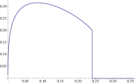
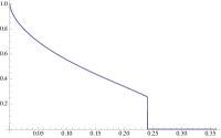
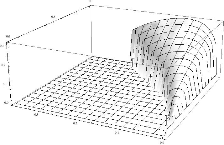
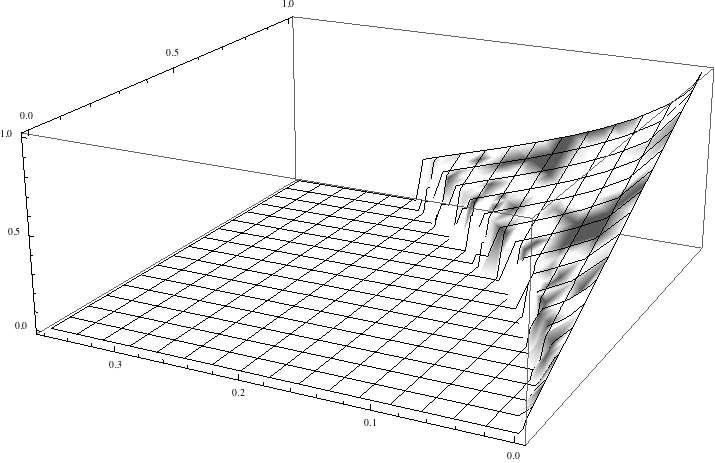
Figure 7. Numerical plots of the typical speed $v(\delta,\beta)$ and the typical charge $\rho(\delta,\beta)$ in Theorems 1.3 and 1.4, based on a $100\times 100$ truncation of the matrix in (1.11), for the case where $\omega_{1}$ is standard normal. Above: plot of $\beta\mapsto v(\delta,\beta)$ and $\beta\mapsto\rho(\delta,\beta)$ for $\delta=1$ and $\beta\in(0,0.36)$. Below: same for $\delta\in(0,1)$ and $\beta\in(0,0.36)$ (for graphical clarity the axes have been rotated: the $\delta$-axis runs from front to back, the $\beta$-axis runs from right to left).

2. Theorems 1.3–1.4 and 1.9 show that the annealed charged polymer exhibits a phase transition of first order. The speed $v(\delta,\beta)$ of the polymer chain is strictly positive in the ballistic phase and zero in the subballistic phase (which explains the names associated with these two phases). In the ballistic phase the speed is given by the spectral formula in (1.25). The latter generalizes the spectral formula derived in Greven and den Hollander [18] for the speed $v(\beta)=v(\infty,\beta)$ of the weakly self-avoiding walk. The charge $\rho(\delta,\beta)$ of the polymer chain is strictly positive in the ballistic phase and zero in the subballistic phase. In the ballistic phase the charge is given by the spectral formula in (1.28). Fig. 7 shows a numerical plot of $\beta\mapsto v(1,\beta)$ and $\beta\mapsto\rho(1,\beta)$ when $\omega_{1}$ is standard normal. Interestingly, the speed is not monotone on $(0,\beta_{c}(1)]$. This is in contrast with the monotonicity that was found (but was not proven) in [18] for the weakly self-avoiding walk (for which $\beta_{c}(\infty)=\infty$). Equally interesting, the charge is monotone on $(0,\beta_{c}(1)]$. A rough heuristics behind the shape of $v(\delta,\beta)$ and $\rho(\delta,\beta)$ is the following. Approximating the distributions of $S_{n}$ and $\Omega_{n}$ by standard normal laws, we get

(1.51) $$F^{*}(\delta,\beta) =\lim_{n\to\infty}\frac{1}{n}\log({\mathbb{E}}^{\delta}\times\mathrm{E})\,\left(\exp\left[-\beta\sum_{x\in\mathbb{Z}}\left(\sum_{i=1}^{n}\omega_{i}\,1_{\{S_{i}=x\}}\right)^{2}+\delta\sum_{i=1}^{n}\omega_{i}\right]\right)$$

$$\approx\sup_{{v\in(0,\infty)}\atop{\rho\in\mathbb{R}}}\left[-\beta v\left(\frac{\rho}{v}\right)^{2}+\delta\rho-\tfrac{1}{2}(v^{2}+\rho^{2})\right].$$

Here, the supremum runs over the possible values of the empirical speed and the empirical charge, the first term arises from the Hamiltonian in (1.8), the second term comes from the tilting of the charges in (1.3), together with the approximation ${\mathbb{E}}^{\delta}(\omega_{1})\approx\delta$, while the third term embodies the normal approximation. For fixed $\rho$ the supremum over $v$ is taken at $v=\beta^{1/3}\rho^{2/3}$. Substitution of this relation shows that the supremum over $\rho$ is taken at the solution of the equation $\rho=\delta-2\beta^{2/3}\rho^{1/3}$. Hence

(1.52) $$v(\delta,\beta)\approx\beta^{\tfrac{1}{3}}\rho(\delta,\beta)^{\tfrac{2}{3}},\qquad\rho(\delta,\beta)\approx\delta-2\beta^{\tfrac{2}{3}}\rho(\delta,\beta)^{\tfrac{1}{3}}.$$

These approximations are compatible with the numerical plots in Fig. 7.

3. Theorem 1.6 identifies the rate functions in the large deviation principles for the speed and the charge. Both rate functions exhibit flat pieces in both phases, as indicated in Figs. 4–5. These flat pieces correspond to an inhomogeneous strategy for the polymer to realise a large deviation. For instance, in the flat piece on the left of Fig. 4, if the speed is $\theta<\widetilde{v}(\delta,\beta)$, then the charge makes a large deviation on a stretch of the polymer of length $\theta/\widetilde{v}(\delta,\beta)$ times the total length, so as to allow it to move at speed $\widetilde{v}(\delta,\beta)$ along that stretch at zero cost, and then makes a large deviation on the remaining stretch, so as to allow it to be subballistic along that remaining stretch at zero cost. For the weakly self-avoiding walk the presence of a flat piece in the rate function for the speed was noted in den Hollander [25, Chapter 8]. It is possible to extend Theorem 1.6 to a joint LDP, but we refrain from doing so.

4. Theorem 1.7 provides the central limit theorem for the speed and the charge in the interior of the ballistic regime. The variance is the inverse of the curvature of the rate function at its unique zero, as is to be expected. Numerical plots are given in Fig. 8. It is hard to obtain accurate simulations for $\beta$ small, but the plots appear to be compatible with the assumption made in (1.48). For weakly self-avoiding walk it was shown in van der Hofstad, den Hollander and König [22, 23] that $\beta\mapsto\sigma_{v}(\beta)^{2}=\sigma_{v}(\infty,\beta)^{2}$ is discontinuous at $\beta=0$, namely, $\lim_{\beta\downarrow 0}\sigma_{v}(\beta)=C_{v}<1=\sigma_{v}(0)$. Fig. 7 suggests that this behaviour persists for $\delta<\infty$. The heuristics is that the variance of the endpoint of the polymer gets squeezed because the polymer moves ballistically. Apparently this squeezing does not vanish as the speeds tends to zero.

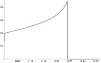
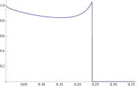
Figure 8. Numerical plots of the variance of the speed $\sigma_{v}(\delta,\beta)^{2}$ and the variance of the charge $\sigma_{\rho}(\delta,\beta)^{2}$ in Theorem 1.7 for the same range of $\beta$ and $\delta$ as in Fig. 7.

We do not deduce the central limit theorem from the large deviation principle, but rather exploit finer properties of the spectral representation for the excess free energy. We have no result about the fluctuations at criticality. We expect these fluctuations to be of order $\sqrt{n}$ in the upward direction and of order $n^{2/3}$ in the downward direction.

5. Theorem 1.8 identifies the scaling behavior of the critical curve for small and for large charge bias. Part (1) shows that the scaling is anomalous for small charge bias, and implies that the critical curve is not analytic at the origin. Part (2) shows that the scaling is also delicate for large charge bias. Heuristically, it is easier to build small absolute values of $\Omega_{\ell}=\sum_{k=1}^{\ell}\omega_{k}$ for small values of $\ell$ when the charge distribution is non-lattice rather than lattice. Since the local times are of order one in the ballistic phase, we expect that the ballistic phase for the lattice case is contained in the ballistic phase for the non-lattice case (because smaller values of $\beta$ are needed to compensate for the larger absolute values of $\Omega_{\ell}$).

6. Theorem 1.10 deals with weak interaction limits. Part (1) shows that near the horizontal axis in Fig. 3 the free energy, the speed and the charge exhibit an anomalous scaling. This is a generalization of the scaling found in van der Hofstad and den Hollander [21] for weakly self-avoiding walk. Part (2) shows that near the origin of Fig. 3 the free energy scales like the distance to the critical curve, provided the latter is approached properly. The constants $A_{\delta},B_{\delta},C_{\delta}$ are expected to represent the free energy, speed and charge of a Brownian version of the charged polymer with Hamiltonian

(1.53) $$H_{T}^{\mathrm{\widetilde{W}}}(W[0,T])=\int_{\mathbb{R}}L_{T}^{\mathrm{\widetilde{W}}}(x)^{2}\,\text{\rm d}x,\quad L_{T}^{\mathrm{\widetilde{W}}}(x)=\int_{0}^{T}\text{\rm d}\mathrm{\widetilde{W}}_{s}\,\delta(W_{s}-x),$$

where $W[0,T]$ is the path of the polymer, $\text{\rm d}\mathrm{\widetilde{W}}_{s}$ is the charge of the interval $\text{\rm d}s$, $\mathrm{\widetilde{W}}[0,T]$ is an independent Brownian motion with drift $\delta$, and the polymer measure has $\beta=1$ with the Wiener measure as reference measure. The version without charges is known as the Edwards model (see van der Hofstad, den Hollander and König [23, 24]). The limit below (1.47) is expected to represent the standard deviation in the central limit theorem as $T\to\infty$ for the charge in the continuum model defined via (1.53).

7. Theorem 1.2 corrects a mistake in den Hollander [26, Chapter 8], where it was argued that $F^{*}\equiv 0$ (i.e., ${\mathcal{S}}$ covers the full quadrant, or $\beta_{c}\equiv 0$). The mistake can be traced back to a failure of convexity of the function $\ell\mapsto G^{*}_{\delta,\beta}(\ell)$. Using the technique outlined in den Hollander [26, Chapter 8], it can be shown that for every $d\geq 1$ and every $(\delta,\beta)\in{\mathcal{S}}$,

(1.54) $$\lim_{n\to\infty}\frac{(\alpha_{n})^{2}}{n}\,\log{\mathbb{Z}}_{n}^{*,\delta,\beta}=-\chi,\quad\mbox{ where }\quad{\mathbb{Z}}_{n}^{*,\delta,\beta}=e^{-f(\delta)n}\,{\mathbb{Z}}_{n}^{\delta,\beta},$$

with $\alpha_{n}=(n/\log n)^{1/(d+2)}$ and with $\chi\in(0,\infty)$ a constant that is explicitly computable. The idea behind (1.54) is the following. For $(\delta,\beta)\in{\mathcal{S}}$ the empirical charge makes a large deviation under the disorder measure ${\mathbb{P}}^{\delta}$ so that it becomes zero. The price for this large deviation is

(1.55) $$e^{-nH({\mathbb{P}}^{0}\,|\,{\mathbb{P}}^{\delta})+o(n)},$$

where $H({\mathbb{P}}^{0}\,|\,{\mathbb{P}}^{\delta})$ denotes the specific relative entropy of ${\mathbb{P}}^{0}={\mathbb{P}}$ with respect to ${\mathbb{P}}^{\delta}$. Since the latter equals $\log M(\delta)=-f(\delta)$ (recall (1.2)–(1.3)), this accounts for the leading term in the free energy. Conditional on the empirical charge being zero, the attraction between charged monomers with the same sign wins from the repulsion between charged monomers with opposite sign, making the polymer chain contract to a subdiffusive scale $\alpha_{n}$. This accounts for the correction term in the free energy. It is shown in [26] that under the annealed polymer measure,

(1.56) $$\left(\frac{1}{\alpha_{n}}\,S_{\lfloor nt\rfloor}\right)_{0\leq t\leq 1}\Longrightarrow(U_{t})_{0\leq t\leq 1},\qquad n\to\infty,$$

where $\Longrightarrow$ denotes convergence in distribution and $(U_{t})_{t\geq 0}$ is a Brownian motion on $\mathbb{R}^{d}$ conditioned not to leave a ball with a certain radius and a certain randomly shifted center.

8. Previous results on the charged polymer model include limit theorems for the Hamiltonian in (1.4). Chen [7] proves an annealed central limit theorem and an annealed law of the iterated logarithm, and identifies the annealed moderate deviations (see also Chen and Khoshnevisan [8]). Asselah [1], [2] derives upper and lower bounds for annealed large deviations. Hu and Khoshnevisan [27] give a law of the iterated logarithm and a strong approximation theorem: on an enlarged probability space the properly normalised Hamiltonian converges almost-surely to a reparametrised Brownian motion. Guillotin-Plantard and dos Santos [19] prove a quenched central limit theorem in dimensions $d=1,2$. Hu, Khoshnevisan and Wouts [28] consider the quenched weak interaction regime (where the Hamiltonian is multiplied by $\beta/n$ rather than $-\beta$) and prove a phase transition from Brownian scaling to four-point localization: for small $\beta$ the polymer behaves like a simple random walk, while for large $\beta$ a large fraction of the monomers are located on four sites.

Figure 9. Qualitative plots of the maps $\beta\mapsto F(\delta,\beta)$ and $u\mapsto I_{\delta}^{H}(u)$. The latter is linear on $[0,K_{\delta}]$ and strictly convex on $(K_{\delta},\infty)$, where $K_{\delta}$ is the constant in (1.45), and tends to zero at infinity.

9. The large deviation bounds derived by Asselah [1], [2] can be completed as follows. Under the annealed polymer measure, the sequence $(n^{-1}H_{n}^{\omega})_{n\in\mathbb{N}}$ (recall (1.8)) satisfies the (weak) large deviation principle on $\mathbb{R}$ with (weak) rate function $I^{H}_{\delta}$ given by (see Fig. 9)

(1.57) $$I^{H}_{\delta}(u)=\sup_{\beta\in(0,\infty)}[-u\beta-F(\delta,\beta)],\qquad u\in\mathbb{R}.$$

Here we use that $F(\delta,\beta)=\infty$ for $\beta\in(-\infty,0)$ and $F(\delta,0)=0$, to restrict the supremum to $\beta\in(0,\infty)$. (Indeed, the strategy where the charges are bounded from below by a positive constant and the walk zigzags between two consecutive sites has an entropic cost that is linear in the length of the polymer, whereas the positive energetic contribution is quadratic.) Since $F(\delta,\beta)=\mu(\delta,\beta)+f(\delta)$ by Theorem 1.1, (1.57) provides us with an explicit variational formula similar to (1.30)–(1.31).

10. Here are some open problems for the quenched version of the model (see Appendix B):

• Does the quenched free energy exist for ${\mathbb{P}}^{\delta}$-a.e. $\omega$, and is it constant? How does it depend on $\delta$ and $\beta$? Trivially, it is convex in $\beta$ for all $\delta$, but what more can be said?

• Is the quenched charged polymer ballistic for all $\delta\in(0,\infty)$? How does the speed depend on $\beta$ and $\delta$?

• In the quenched model with $\delta=0$, is the polymer chain subdiffusive (like in the annealed model; see item 3 above)? The fluctuations of the charges are expected to push the polymer farther apart than in the annealed model. Is there a scaling limit for ${\mathbb{P}}$-a.e. $\omega$, or does the polymer chain fluctuate so much that there is a scaling limit only along $\omega$-dependent subsequences (“sample dependence”)?

11. Still looking at a quenched model, Derrida, Griffiths and Higgs [12] and Derrida and Higgs [13] consider the case where the steps of the random walk are drawn from $\{0,1\}$ rather than $\{-1,+1\}$, which makes the model a bit more tractable, both theoretically and numerically. In [12] the charge disorder is binary, and numerical evidence is found for the free energy to be self-averaging and to exhibit a freezing transition at a critical threshold $\beta_{c}\in(0,\infty)$, i.e., the quenched charged polymer is ballistic when $0\leq\beta<\beta_{c}$ and subballistic when $\beta>\beta_{c}$. In the latter phase numerical simulation shows that the end-to-end distance scales like $n^{\nu}$, with $\nu=\nu(\beta)$ an exponent that depends on $\beta$. In this phase, long and rare stretches of the polymer that are globally neutral find it energetically favorable to collapse onto single sites. Numerical simulation indicates that $\beta_{c}\geq 0.48$. In [13] the charge disorder is standard normal and the total charge $\sum_{i=1}^{n}\omega_{i}$ is conditioned to grow like $n^{\xi}$, $\xi\in[-\frac{1}{2},1]$. It is found numerically that the end-to-end distance scales like $n^{\nu}$, with $\nu=\nu(\xi)$ an exponent that depends on $\xi$ and grows roughly linearly from $\nu(-\frac{1}{2})=0$ to $\nu(1)=1$, with $\nu(\frac{1}{2})\approx 0.574$. The latter is the exponent for the quenched charged polymer when the charges are typical.

12. It would be interesting to deal with charges whose interaction extends beyond the ‘on-site’ interaction in (1.4), like a Coulomb potential (polynomial decay) or a Yukawa potential (exponential decay). A Yukawa potential arises from a Coulomb potential via screening of the charges when the polymer chain is immersed in an ionic fluid.

13. Biskup and König [6], Ioffe and Velenik [29], Kosygina and Mountford [34] deal with annealed versions of various models of simple random walk in a random potential. In all these models the interaction is either attractive or repulsive, meaning that the annealed partition function is the expectation of the exponential of a functional of the local times of simple random walk that is either subadditive or superadditive. As we will see in Section 2, our annealed charged polymer model is neither attractive nor repulsive. However, our spectral representation is flexible so as to include such models.

2. Spectral representation for the free energy

Our goal in this section is to prove Theorem 1.1, i.e., the existence of the annealed free energy and its characterization in terms of an eigenvalue problem. In Section 2.1 we show that the edge-crossing numbers of the simple random walk have a Markovian structure. In Section 2.2 we rewrite the annealed partition function as the expectation of a functional of the local times of the simple random walk, which are a two-block functional of the edge-crossing numbers. In Section 2.3 we introduce the generating function of the annealed excess partition function, and show that this can be expressed in terms of the matrices defined in (1.11)–(1.12). The annealed excess free energy is the radius of convergence of this generating function. In Section 2.4 we analyze the spectral radii of the matrices. In Section 2.5 we identify the annealed excess free energy in terms of these spectral radii. In Section 2.6 we put everything together to prove Theorem 1.1.

This section is the cornerstone of the following sections, since the representation of the partition function developed here will be used throughout the paper.

2.1. Markov property of the edge-crossing numbers

The observation that the edge-crossing numbers of the simple random walk have a Markovian property goes back at least to Knight [32]. This property can be formulated in various ways. In this section we present a version that holds for a fixed time horizon, which is based on the well-known link between random walk excursions and rooted planar trees (see Remark 2.5 below).

We work conditionally on the event $\{S_{n}=x\}$ for fixed $n\in\mathbb{N}_{0}$ and $x\in\mathbb{Z}$, and w.l.o.g. we assume that $x\in\mathbb{N}_{0}$. Then all edges are crossed the same number of times upwards and downwards, except for the edges in the stretch $\{0,\ldots,x\}$, which have one extra upward crossing. We define the edge-crossing number $M^{+}_{y}$, $y\in\mathbb{N}_{0}$, as the number or upward crossing of the edge $(y,y+1)$ that are eventually followed by a downward crossing (i.e., we disregard the last upward crossing for $0\leq y<x$). To keep the notation symmetric, we define $M^{-}_{y}$, $y\in\mathbb{N}_{0}$, as the number of downward crossings of the edge $(-y-1,-y)$, each of which necessarily is eventually followed by an upward crossing. In formulas,

(2.1) $$M^{+}_{y}=\Bigg{\lfloor}\frac{1}{2}\sum_{k=1}^{n}{\sf 1}_{\big{\{}\{S_{k-1},S_{k}\}=\{y,y+1\}\big{\}}}\Bigg{\rfloor},\quad M^{-}_{y}=\Bigg{\lfloor}\frac{1}{2}\sum_{k=1}^{n}{\sf 1}_{\big{\{}\{S_{k-1},S_{k}\}=\{-y,-1-y\}\big{\}}}\Bigg{\rfloor},\quad y\in\mathbb{N}_{0}.$$

For ease of notation we suppress the dependence on $n$.

Remark 2.1.

In what follows we will work with the local times of the random walk, i.e., the site visit numbers defined by

(2.2) $$L_{n}(x)=\sum_{i=1}^{n}{\sf 1}_{\{S_{i}=x\}},\qquad n\in\mathbb{N},\,x\in\mathbb{Z}.$$

These can be expressed in terms of the edge-crossing numbers as follows:

(2.3) $$\text{On the event }\{S_{n}=x\}\text{ with }x\in\mathbb{N}_{0}\colon\quad L_{n}(y)=\begin{cases}M^{+}_{y-1}+M^{+}_{y},&\text{if }y>x,\\ M^{+}_{y-1}+M^{+}_{y}+1,&\text{if }1\leq y\leq x,\\ M^{+}_{0}+M^{-}_{0},&\text{if }y=0,\\ M^{-}_{-y-1}+M^{-}_{-y},&\text{if }y<0.\end{cases}$$

We next define a specific branching process, which will be shown to be closely linked to the edge-crossing numbers $M^{\pm}_{y}$, $y\in\mathbb{N}_{0}$.

Definition 2.2.

Fix $\ell,x\in\mathbb{N}_{0}$. Define a two-species branching process

(2.4) $$(M^{+},M^{-})=(M^{+}_{y},M^{-}_{y})_{y\in\mathbb{N}_{0}}$$

with law ${\mathcal{P}}_{\ell,x}$ as follows:

• At generation 0 there are $\ell$ individuals, which are divided by fair coin tossing into two subpopulations, labelled $+$ and $-$.

• Each subpopulation evolves independently as a critical Galton-Watson branching process with a geometric offspring distribution, denoted by $\mathrm{Geo}_{0}(\frac{1}{2})$ and given by $\mathrm{Geo}_{0}(\frac{1}{2})(i)=2^{-(i+1)}$, $i\in\mathbb{N}_{0}$.

• If $x\in\mathbb{N}$, then there is additional immigration of a $\mathrm{Geo}_{0}(\frac{1}{2})$-distributed number of individuals in the $+$ subpopulation, at each generation $1,\dots,x$ (equivalently, the generations $0,\dots,x-1$ have an additional “hidden” individual, which is not counted but produces offspring).

• Define $M^{\pm}_{y}$ as the size of the $\pm$ subpopulation in the $y$-th generation.

Define the total population size

(2.5) $$\Xi=\sum_{y\in\mathbb{N}_{0}}(M^{+}_{y}+M^{-}_{y})$$

and note that $\Xi<\infty$ a.s. because a critical Galton-Watson process eventually dies out.

We can now state the main result of this section. Abbreviate $L_{0}=L_{n}(0)$.

Theorem 2.3.

Fix $\ell,n,x\in\mathbb{N}_{0}$ such that $0\leq\ell\leq\frac{1}{2}n$, $0\leq x\leq n$ and $x-n$ is even. The edge-crossing numbers $(M^{+},M^{-})$ of the simple random walk defined in (2.1) conditionally on $\{L_{0}=\ell,S_{n}=x\}$ have the same joint distribution as the branching process with law ${\mathcal{P}}_{\ell,x}$ defined in Definition 2.2 conditionally on $\{\Xi=\frac{1}{2}(n-x)\}$. In formulas,

(2.6) $$\mathrm{P}\Big{(}(M^{+},M^{-})=(m^{+},m^{-}),\,L_{0}=\ell,\,S_{n}=x\Big{)}$$

$$\qquad={\mathcal{P}}_{\ell,x}\Big{(}(M^{+},M^{-})=(m^{+},m^{-}),\,\Xi=\tfrac{1}{2}(n-x)\Big{)},$$

for all sequences $(m^{+},m^{-})=(m^{+}_{y},m^{-}_{y})_{y\in\mathbb{N}_{0}}\in(\mathbb{N}_{0}\times\mathbb{N}_{0})^{\mathbb{N}_{0}}$.

Remark 2.4.

Taking the scaling limit of (2.6) we obtain the famous Ray-Knight relation between Brownian motion local time and squared Bessel processes (see Revuz and Yor  [37]). We refer to Tóth [39, 40] for analogous relations involving more general processes, arising in the context of self-interacting random walks.

Before proving Theorem 2.3, we note that the transition kernel of a critical Galton-Watson branching process with geometric offspring distibution is given by the matrix $Q(i,j)$, $i,j\in\mathbb{N}_{0}$, defined in (1.9). In fact, if $(\xi_{n})_{n\in\mathbb{N}}$ are i.i.d. $\mathrm{Geo}_{0}(\frac{1}{2})$ random variables, then

(2.7) $$Q(i,j)=\begin{cases}{\sf 1}_{\{j=0\}},&\text{if }i=0,\ j\in\mathbb{N}_{0},\\ \rule{0.0pt}{20.00003pt}\displaystyle\binom{i+j-1}{i-1}\left(\frac{1}{2}\right)^{i+j}=P(\xi_{1}+\ldots+\xi_{i}=j),&\text{if }i\in\mathbb{N},\ j\in\mathbb{N}_{0},\end{cases}$$

In the presence of immigration, the transition kernel becomes $Q(i+1,j)$.

By Definition 2.2, $(M^{+},M^{-})$ is a Markov chain on $\mathbb{N}_{0}\times\mathbb{N}_{0}$ that is not time-homogeneous whenever $x\neq 0$ (due to the immigration). The initial distribution of this Markov chain is

(2.8) $${\mathcal{P}}_{\ell,x}\big{(}(M^{+}_{0},M^{-}_{0})=(a,b)\big{)}=\rho_{\ell}(a,b)\quad\text{ with }\quad\rho_{\ell}(a,b)=\binom{\ell}{a}\,\frac{1}{2^{\ell}}\,{\sf 1}_{\{a+b=\ell\}},\quad a,b\in\mathbb{N}_{0},$$

while the transition kernel factorizes, i.e., it is the product of its marginals, because conditionally on $(M^{+}_{0},M^{-}_{0})$ the two components $(M^{+}_{y})_{y\in\mathbb{N}}$ and $(M^{-}_{y})_{y\in\mathbb{N}}$ evolve independently, with marginal transition kernels

(2.9) $$\begin{split}{\mathcal{P}}_{\ell,x}\big{(}M^{+}_{y+1}=j\mid M^{+}_{y}=i\big{)}&=Q(i+1,j)\,{\sf 1}_{\{y<x\}}+Q(i,j)\,{\sf 1}_{\{y\geq x\}},\\ {\mathcal{P}}_{\ell,x}\big{(}M^{-}_{y+1}=j\mid M^{-}_{y}=i\big{)}&=Q(i,j),\qquad i,j\in\mathbb{N}_{0}.\end{split}$$

We are now ready to give the proof of Theorem 2.3.

Proof.

Note that both sides of (2.6) vanish, unless the sequences $m^{\pm}$ satisfy the conditions

(2.10) $$m_{0}^{+}+m_{0}^{-}=\ell\,,\qquad\sum_{y\in\mathbb{N}_{0}}(m_{y}^{+}+m_{y}^{-})=\frac{1}{2}(n-x).$$

The first condition holds because $L_{0}=M_{0}^{+}+M_{0}^{-}$ for the random walk (each visit to zero is preceded by a crossing of either $(0,1)$ or $(-1,0)$), while ${\mathcal{P}}_{\ell,x}(M_{0}^{+}+M_{0}^{-}=\ell)=1$ for the branching process by construction. Analogously, the second condition in (2.10) holds for the branching process by the definition of $\Xi$ in (2.5), while it holds for the random walk, because the total number of steps $n$ equals the total number of upward or downward crossings, which is given by $2\sum_{y\in\mathbb{N}_{0}}(M^{+}_{y}+M^{-}_{y})+x$ (recall that the last upward crossing of a bond in the stretch $\{0,\ldots,x\}$ is not counted in $M^{+}_{y}$).

Henceforth we fix two sequences $(m^{+},m^{-})=(m^{+}_{y},m^{-}_{y})_{y\geq 0}\in(\mathbb{N}_{0}\times\mathbb{N}_{0})^{\mathbb{N}_{0}}$ that satisfy (2.10). Below we will show that the number of simple random walk paths $(S_{1},\ldots,S_{n})$ contributing to the event $\{(M^{+},M^{-})=(m^{+},m^{-}),\,S_{n}=x,\,L_{0}=\ell\}$ equals

(2.11) $$\binom{\ell}{m_{0}^{+}}\,\prod_{y=0}^{x-1}C(m_{y}^{+}+1,m_{y+1}^{+})\,\prod_{y\geq x}C(m_{y}^{+},m_{y+1}^{+})\,\prod_{y\geq 0}C(m_{y}^{-},m_{y+1}^{-})\,,$$

where

(2.12) $$C(0,j)={\sf 1}_{\{j=0\}},\quad j\in\mathbb{N}_{0},\qquad C(i,j)=\binom{i+j-1}{i-1}\quad i\in\mathbb{N},\,j\in\mathbb{N}_{0}.$$

The first product in (2.11) is $1$ when $x=0$, by convention. Note that $m^{\pm}$ have a finite sum by (2.10), and hence are eventually zero: $m^{\pm}_{y}=0$ for large enough $y$. Since $C(0,0)=1$, this means that the products in (2.11) are finite.

We can now prove (2.6). The probability in the left-hand side of (2.6) is obtained after dividing (2.11) by $2^{n}$, which is the total number of random walk paths. Recalling (1.9), (2.8) and (2.10), we obtain

(2.13) $$\begin{split}&\mathrm{P}\Big{(}(M^{+},M^{-})=(m^{+},m^{-}),\,L_{0}=\ell,\,S_{n}=x\Big{)}\\ &\qquad=\rho_{\ell}(m_{0}^{+},m_{0}^{-})\,\prod_{y=0}^{x-1}Q(m_{y}^{+}+1,m_{y+1}^{+})\,\prod_{y\geq x}Q(m_{y}^{+},m_{y+1}^{+})\,\prod_{y\geq 0}Q(m_{y}^{-},m_{y+1}^{-}),\end{split}$$

which is precisely the probability in the right-hand side of (2.6), by the Markov property of the process $(M^{+},M^{-})$ under the law ${\mathcal{P}}_{\ell,x}$ (recall (2.8)-(2.9)).

It remains to prove (2.11). Observe that $C(i,j)$ in (2.12) equals the number of ways in which $j$ objects can be allocated to $i$ boxes, i.e., the number of sequences $(a_{1},\ldots,a_{i})\in(\mathbb{N}_{0})^{i}$ satisfying $a_{1}+\ldots+a_{i}=j$. As to the random walk, the crossing number $m_{0}^{-}$ counts the number of excursions below $0$, while the crossing number $m_{1}^{-}$ counts the number of excursions below $-1$. The key observation is that each excursion below $-1$ is included in precisely one excursion below $0$. Therefore the number of ways in which the $m_{1}^{-}$ excursions below $-1$ can be “allocated” to the $m_{0}^{-}$ excursions below $0$ equals $C(m_{0}^{-},m_{1}^{-})$. Iterating this argument, we see that the last product in (2.11) counts the number of random walk paths in the negative half-plane that are compatible with the given bond crossing-numbers $(m^{-}_{y})_{y\in\mathbb{N}_{0}}$.

For the positive part of the random walk path there is one difference. When $x\in\mathbb{N}$, each of the $m^{+}_{1}$ excursions above $+1$ can be allocated not only to the $m^{+}_{0}$ excursions above $0$, but also to the last incomplete excursion leading to $x$. This explains the presence of “$+1$” in the combinatorial factor $C(m_{0}^{+}+1,m_{1}^{+})$ in (2.11). This holds until level $x$, while above level $x$ the combinatorial factor $C(m^{+}_{y},m^{+}_{y+1})$ applies. The first two products in (2.11) therefore count the number of random walk paths in the positive half-plane that lead to $x$ and are compatible with the given bond crossing-numbers $(m^{+}_{y})_{y\in\mathbb{N}_{0}}$.

It remains to combine the positive and the negative parts of the random walk path we have just built. This can be done by alternating the $m_{0}^{+}$ positive excursions and the $m^{-}_{0}$ negative excursions in an arbitrary way, while preserving their relative order. Since $m^{+}_{0}+m^{-}_{0}=\ell$, this can be done in $\binom{\ell}{m_{0}^{+}}$ ways, which leads to the first factor in (2.11). ∎

Remark 2.5.

One way to visualize (2.11) is to identify a random walk excursion with a planar rooted tree (the random walk path traces out the “external boundary” of the tree). With this identification, the bond-crossing numbers $(m_{y})_{y\in\mathbb{N}_{0}}$ represent the number of branches of the tree at level $y\in\mathbb{N}_{0}$, and the number of such trees is given by $\prod_{i\in\mathbb{N}_{0}}C(m_{i},m_{i+1})$.

2.2. From the annealed partition function to functionals of local times

The first step in our analysis of the free energy is to rewrite the annealed partition function as the partition function of the simple random walk weighted by a functional of its local times $L_{n}(y)$ defined in (2.2). To that end we define, for $\ell\in\mathbb{N}_{0}$ and $(\delta,\beta)\in{\mathcal{Q}}$,

(2.14) $$G_{\delta,\beta}(\ell)=\log{\mathbb{E}}^{\delta}\left[e^{-\beta\Omega_{\ell}^{2}}\right].$$

Note that $\Omega_{0}=0$, so that $G_{\delta,\beta}(0)=0$.

Lemma 2.6.

For $n\in\mathbb{N}$ and $(\delta,\beta)\in{\mathcal{Q}}$,

(2.15) $${\mathbb{Z}}_{n}^{\delta,\beta}=\mathrm{E}\left[\exp\left\{\sum_{x\in{\mathbb{Z}}}G_{\delta,\beta}(L_{n}(x))\right\}\right].$$

Proof.

Rewrite (1.7) as

(2.16) $${\mathbb{Z}}_{n}^{\delta,\beta}=({\mathbb{E}}^{\delta}\times\mathrm{E})\left[\prod_{x\in{\mathbb{Z}}}\exp\left\{-\beta\left(\sum_{i=1}^{n}\omega_{i}{\sf 1}_{\{S_{i}=x\}}\right)^{2}\right\}\right]=\mathrm{E}\left[\,\prod_{x\in{\mathbb{Z}}}{\mathbb{E}}^{\delta}\left[e^{-\beta\Omega_{L_{n}(x)}^{2}}\right]\right],$$

and use (2.14). ∎

Depending on which phase we are working in, it will be convenient to also use the function $G^{*}_{\delta,\beta}(\ell)$ defined by

(2.17) $$G^{*}_{\delta,\beta}(\ell)=G_{\delta,\beta}(\ell)-f(\delta)\ell,\qquad\ell\in\mathbb{N}_{0},$$

which equals (1.10) by (2.14) (recall (1.3) and (1.14)), and to rewrite Lemma 2.6 as

(2.18) $${\mathbb{Z}}_{n}^{*,\delta,\beta}=({\mathbb{E}}\times\mathrm{E})\left[e^{\sum_{x\in\mathbb{Z}}\big{(}\delta\Omega_{L_{n}(x)}-\beta\Omega_{L_{n}(x)}^{2}\big{)}}\right]=\mathrm{E}\left[\exp\left\{\sum_{x\in{\mathbb{Z}}}G^{*}_{\delta,\beta}(L_{n}(x))\right\}\right]$$

with (recall (1.54))

(2.19) $${\mathbb{Z}}_{n}^{*,\delta,\beta}=e^{-f(\delta)n}\,{\mathbb{Z}}_{n}^{\delta,\beta}.$$

In Appendix A we collect some properties of $G^{*}_{\delta,\beta}$ that will be needed along the way.

Example: If the marginal of ${\mathbb{P}}$ is standard normal, then by direct computation

(2.20) $$G^{*}_{\delta,\beta}(\ell)=-\tfrac{1}{2}\log(1+2\beta\ell)+\tfrac{1}{2}\,\delta^{2}\,\frac{\ell}{1+2\beta\ell}.$$

Remark: We close this section with the following observation. In Section 1.2 we argued that working with (1.8) rather than (1.4) as the interaction Hamiltonian amounts to replacing $\beta$ by $2\beta$ and adding a charge bias. Indeed, this is immediate from the relation

(2.21) $$2\sum_{1\leq i<j\leq n}\omega_{i}\omega_{j}\,{\sf 1}_{\{S_{i}=S_{j}\}}=\sum_{x\in\mathbb{Z}^{d}}\left(\sum_{i=1}^{n}\omega_{i}\,{\sf 1}_{\{S_{i}=x\}}\,\right)^{2}-\sum_{i=1}^{n}\omega_{i}^{2}.$$

For the annealed model, the last sum is not constant (unless $\omega_{i}=\pm 1$). To handle this, define $\bar{{\mathbb{P}}}^{\beta}$ as the product law with marginal given by

(2.22) $$\bar{{\mathbb{P}}}^{\beta}(d\omega_{1})=\frac{e^{\beta\omega_{1}^{2}}\,{\mathbb{P}}(\text{\rm d}\omega_{1})}{\bar{M}(\beta)},\qquad\bar{M}(\beta)={\mathbb{E}}(e^{\beta\omega_{1}^{2}}),$$

where we need to assume that $\bar{M}(\beta)<\infty$ for all $\beta\in(0,\infty)$. We put

(2.23) $$\bar{G}_{\delta,\beta}(\ell)=\log\bar{{\mathbb{E}}}^{\beta}\left[e^{\delta\Omega_{\ell}-\beta\Omega_{\ell}^{2}}\right],$$

which is the same as (1.10) but with $\bar{{\mathbb{E}}}^{\beta}$ instead of ${\mathbb{E}}$, and we define the partition function

(2.24) $$\bar{{\mathbb{Z}}}_{n}^{\delta,\beta}=\mathrm{E}\left[e^{\sum_{x\in\mathbb{Z}^{d}}\bar{G}_{\delta,\beta}(L_{n}(x))}\right].$$

Including the last sum in (2.21) amounts to switching from ${\mathbb{Z}}_{n}^{*,\delta,\beta}$ to $\bar{{\mathbb{Z}}}_{n}^{\delta,\beta}$. As mentioned in Section 1.2, in this paper we work with the Hamiltonian without the last sum. The reader may check that $\bar{G}_{\delta,\beta}$ has the same qualitative properties as $G^{*}_{\delta,\beta}$, so that all the computations carried out below can be easily transferred.

2.3. Grand-canonical representation

To compute the annealed free energy we use the generating function associated with the sequence of excess annealed partition functions, i.e.,

(2.25) $${\mathcal{Z}}(\mu,\delta,\beta)=\sum_{n\in\mathbb{N}_{0}}e^{-\mu n}\,{\mathbb{Z}}_{n}^{*,\delta,\beta},\qquad\mu\in[0,\infty),$$

where ${\mathbb{Z}}_{0}^{*,\delta,\beta}=1$. The main result of this section is the following matrix representation of ${\mathcal{Z}}(\mu,\delta,\beta)$. Recall the matrices $A_{\mu,\delta,\beta}(i,j)$ and $\widetilde{A}_{\mu,\delta,\beta}(i,j)$ defined in (1.11)–(1.12), and introduce an extra matrix

(2.26) $$\widehat{A}_{\mu,\delta,\beta}(i,j)=e^{-\mu(i+j)+G^{*}_{\delta,\beta}(i+j)}\,Q(i+1,j),\qquad i,j\in\mathbb{N}_{0}.$$

Proposition 2.7.

For $\mu\in[0,\infty)$ and $(\delta,\beta)\in{\mathcal{Q}}$,

(2.27) $${\mathcal{Z}}(\mu,\delta,\beta)=\left[\frac{1}{1-\widetilde{A}^{\intercal}_{\mu,\delta,\beta}}\,\widehat{A}_{\mu,\delta,\beta}\,\frac{1+A_{\mu,\delta,\beta}}{1-A_{\mu,\delta,\beta}}\,\frac{1}{1-\widetilde{A}_{\mu,\delta,\beta}}\right](0,0).$$

Proof.

To lighten the notation, we suppress the dependence on $\mu,\delta,\beta$. Recalling (2.18), we can write

(2.28) $${\mathcal{Z}}=\sum_{n\in\mathbb{N}_{0}}e^{-\mu n}\,\sum_{(\ell,x)\in(\mathbb{N}_{0})^{2}}\,\big{(}1+{\sf 1}_{\{x>0\}}\big{)}\mathrm{E}\Bigg{[}\exp\Bigg{\{}\sum_{y\in{\mathbb{Z}}}G^{*}(L_{n}(y))\Bigg{\}}{\sf 1}_{\{L_{0}=\ell,S_{n}=x\}}\Bigg{]}\,,$$

where ${\sf 1}_{\{x>0\}}$ accounts for the contribution of $\{S_{n}=-x\}$, which is the same as the contribution of $\{S_{n}=x\}$. Recalling (2.3), we can write

(2.29) $$\begin{split}{\mathcal{Z}}&=\sum_{(\ell,x)\in(\mathbb{N}_{0})^{2}}\,\big{(}1+{\sf 1}_{\{x>0\}}\big{)}\,\sum_{n\in\mathbb{N}_{0}}\,\sum_{(m^{+},m^{-})\in(\mathbb{N}_{0}\times\mathbb{N}_{0})^{\mathbb{N}_{0}}}\\ &\mathrm{P}\big{(}(M^{+},M^{-})=(m^{+},m^{-}),\,L_{0}=\ell,S_{n}=x\big{)}\\ &\qquad\times e^{-\mu n}\,e^{G^{*}(m_{0}^{+}+m_{0}^{-})}\prod_{y=0}^{x-1}e^{G^{*}(m^{+}_{y}+m^{+}_{y+1}+1)}\prod_{y\geq x}e^{G^{*}(m^{+}_{y}+m^{+}_{y+1})}\prod_{y\geq 0}e^{G^{*}(m^{-}_{y}+m^{-}_{y+1})}\,.\end{split}$$

Next we apply Theorem 2.3 to rewrite the probability in the right-hand side of (2.29) as a product of $Q$ matrices, as in (2.13). In order to do this, we must restrict to sequences $(m^{+},m^{-})$ satisfying the two conditions in (2.10). Thus, we define

(2.30) $$\begin{split}{\mathcal{S}}_{\ell,x,n}=\bigg{\{}(m^{+}_{y},m^{-}_{y})_{y\geq 0}\in(\mathbb{N}_{0}\times\mathbb{N}_{0})^{\mathbb{N}_{0}}\colon\,m^{+}_{0}+m^{-}_{0}=\ell,\,\sum_{y\in\mathbb{N}_{0}}(m^{+}_{y}+m^{-}_{y})=\tfrac{1}{2}(n-x)\bigg{\}},\end{split}$$

and restrict the sum over $(m^{+},m^{-})$ in (2.29) to the set ${\mathcal{S}}_{\ell,x,n}$. At this point we combine the definitions of the matrix $Q$, the function $G^{*}$ and the factor $\mu$ into the matrix $A$ defined in (1.11):

(2.31) $$A(i,j)=e^{G^{*}(i+j+1)-\mu(i+j+1)}Q(i+1,j),\qquad i,j\in\mathbb{N}_{0}.$$

We also introduce an extra matrix $\widetilde{A}^{\prime}$ by

(2.32) $$\widetilde{A}^{\prime}(i,j)=e^{G^{*}(i+j)-\mu(i+j)}Q(i,j),\qquad i,j\in\mathbb{N}_{0},$$

which almost coincides with the matrix $\widetilde{A}$ introduced in (1.12), the difference being that $\widetilde{A}^{\prime}(0,0)=1$ while $\widetilde{A}(0,0)=0$. Altogether, we can rewrite (2.29) as (recall (2.8))

(2.33) $$\begin{split}{\mathcal{Z}}=&\sum_{(\ell,x)\in(\mathbb{N}_{0})^{2}}\,\big{(}1+{\sf 1}_{\{x>0\}}\big{)}\sum_{n\in\mathbb{N}_{0}}\,\sum_{(m^{+},m^{-})\in{\mathcal{S}}_{\ell,x,n}}\\ &\qquad\ e^{G^{*}(\ell)-\mu\ell}\,\rho_{\ell}(m_{0}^{+},m_{0}^{-})\prod_{y=0}^{x-1}A(m^{+}_{y},m^{+}_{y+1})\prod_{y\geq x}\widetilde{A}^{\prime}(m^{+}_{y},m^{+}_{y+1})\prod_{y\geq 0}\widetilde{A}^{\prime}(m^{-}_{y},m^{-}_{y+1}).\end{split}$$

Next we introduce the set of sequences $m^{\pm}$ that are eventually zero and satisfy $m^{+}_{0}+m^{-}_{0}=\ell$:

(2.34) $${\mathcal{T}}_{\ell}=\bigg{\{}(m^{+}_{y},m^{-}_{y})_{y\in\mathbb{N}_{0}}\in(\mathbb{N}_{0}\times\mathbb{N}_{0})^{\mathbb{N}_{0}}\colon\,m^{+}_{0}+m^{-}_{0}=\ell,\,m^{\pm}_{y}=0\text{ for large enough $y$}\bigg{\}},$$

and observe that, for every fixed $x\in\mathbb{N}_{0}$,

(2.35) $$\bigcup_{n\in\mathbb{N}_{0}}{\mathcal{S}}_{\ell,x,n}={\mathcal{T}}_{\ell}.$$

The inclusion ${\mathcal{S}}_{\ell,x,n}\subseteq{\mathcal{T}}_{\ell}$ is obvious because sequences in ${\mathcal{S}}_{\ell,x,n}$ are integer-valued with a finite sum and hence are eventually zero. Conversely, if $m^{\pm}$ are eventually zero, then $\sum_{y\in\mathbb{N}_{0}}(m^{+}_{y}+m^{-}_{y})=\tfrac{1}{2}(n-x)$ for some $n\in\mathbb{N}_{0}$. This means that

(2.36) $$\begin{split}\sum_{n\in\mathbb{N}_{0}}\,&\sum_{(m^{+},m^{-})\in{\mathcal{S}}_{\ell,x,n}}\big{(}\ldots\big{)}=\sum_{(m^{+},m^{-})\in{\mathcal{T}}_{\ell}}\big{(}\ldots\big{)}\\ &=\sum_{(m^{+}_{0},\ldots,m^{+}_{x-1})\in(\mathbb{N}_{0})^{x-1}}\;\sum_{\begin{subarray}{c}(t,s)\in(\mathbb{N}_{0})^{2}\\ t\geq x\end{subarray}}\;\sum_{\begin{subarray}{c}(m^{+}_{x},\ldots,m^{+}_{t-1})\in\mathbb{N}^{t-x}\\ (m^{-}_{0},\ldots,m^{-}_{s-1})\in\mathbb{N}^{s}\end{subarray}}{\sf 1}_{\{m_{0}^{+}+m_{0}^{-}=\ell\}}\big{(}\ldots\big{)},\end{split}$$

where the last line provides a convenient parametrization of the set ${\mathcal{T}}_{\ell}$:

• Sum over all possible values of $(m^{+}_{0},\ldots,m^{+}_{x-1})$ (when $x\in\mathbb{N}$).

• Denote by $t$ the smallest value of $y\geq x$ for which $m^{+}_{y}=0$. Likewise denote by $s$ the smallest value of $y\geq 0$ for which $m^{-}_{y}=0$, so that by construction $(m^{+}_{x},\ldots,m^{+}_{t-1})$ and $(m^{-}_{0},\ldots,m^{-}_{s-1})$ can only take values in $\mathbb{N}$.

• It is implicit that $m^{+}_{y}=0$ for $y\geq t$ and $m^{-}_{y}=0$ for $y\geq s$.

We now apply (2.36) to (2.33). We further split ${\mathcal{Z}}={\mathcal{Z}}_{0}+{\mathcal{Z}}_{+}$, where ${\mathcal{Z}}_{0}$ is the contribution of the single term $x=0$, while ${\mathcal{Z}}_{+}$ is the sum $\sum_{x\in\mathbb{N}}(\cdots)$. Observing that

(2.37) $$\tfrac{1}{2}\sum_{\ell\in\mathbb{N}_{0}}e^{G^{*}(\ell)-\mu\ell}\,\rho_{\ell}(m_{0}^{+},m_{0}^{-})=\widehat{A}(m_{0}^{-},m_{0}^{+})$$

by (2.8) and (2.26), we have (with $m^{+}_{t}=m^{-}_{s}=0$ by convention)

(2.38) $$\begin{split}{\mathcal{Z}}_{0}=&\sum_{(t,s)\in(\mathbb{N}_{0})^{2}}\;\sum_{\begin{subarray}{c}(m^{+}_{0},\ldots,m^{+}_{t-1})\in\mathbb{N}^{t}\\ (m^{-}_{0},\ldots,m^{-}_{s-1})\in\mathbb{N}^{s}\end{subarray}}\widehat{A}(m_{0}^{-},m_{0}^{+})\,\prod_{y=0}^{t-1}\widetilde{A}^{\prime}(m^{+}_{y},m^{+}_{y+1})\prod_{y=0}^{s-1}\widetilde{A}^{\prime}(m^{-}_{y},m^{-}_{y+1})\end{split}$$

and

(2.39) $$\begin{split}{\mathcal{Z}}_{+}=\,2\sum_{x\in\mathbb{N}}\,&\sum_{\begin{subarray}{c}(t,s)\in(\mathbb{N}_{0})^{2}\\ t\geq x\end{subarray}}\;\sum_{(m^{+}_{0},\ldots,m^{+}_{x-1})\in(\mathbb{N}_{0})^{x-1}}\;\sum_{\begin{subarray}{c}(m^{+}_{x},\ldots,m^{+}_{t-1})\in\mathbb{N}^{t-x}\\ (m^{-}_{0},\ldots,m^{-}_{s-1})\in\mathbb{N}^{s}\end{subarray}}\\ &\widehat{A}(m_{0}^{-},m_{0}^{+})\,\prod_{y=0}^{x-1}A(m^{+}_{y},m^{+}_{y+1})\prod_{y=x}^{t-1}\widetilde{A}^{\prime}(m^{+}_{y},m^{+}_{y+1})\prod_{y=0}^{s-1}\widetilde{A}^{\prime}(m^{-}_{y},m^{-}_{y+1}).\end{split}$$

Finally, we observe that we can replace $\widetilde{A}^{\prime}(i,j)$ by $\widetilde{A}(i,j)$ in (2.38)–(2.39), because for $i\in\mathbb{N}$ these two matrices coincide. After this replacement, the ranges $\mathbb{N}^{t-x}$ and $\mathbb{N}^{s}$ in the sums can be replaced by $(\mathbb{N}_{0})^{t-x}$ and $(\mathbb{N}_{0})^{s}$, respectively, because $\widetilde{A}(0,j)=0$. This leads us to the desired matrix product representations:

(2.40) $$\begin{split}{\mathcal{Z}}_{0}=\sum_{(t,s)\in(\mathbb{N}_{0})^{2}}\;\big{[}(\widetilde{A}^{\intercal})^{s}\,\widehat{A}\,\widetilde{A}^{t}\big{]}(0,0)=\bigg{[}\frac{1}{1-\widetilde{A}^{\intercal}}\,\widehat{A}\,\frac{1}{1-\widetilde{A}}\bigg{]}(0,0)\end{split}$$

and

(2.41) $$\begin{split}{\mathcal{Z}}_{+}&=2\sum_{x\in\mathbb{N}}\,\sum_{\begin{subarray}{c}(t,s)\in(\mathbb{N}_{0})^{2}\\ t\geq x\end{subarray}}\;\big{[}(\widetilde{A}^{\intercal})^{s}\,\widehat{A}\,A^{x}\,\widetilde{A}^{t-x}\big{]}(0,0)\\ &=\bigg{[}\frac{1}{1-\widetilde{A}^{\intercal}}\,\frac{A}{1-A}\,\widehat{A}\,\frac{1}{1-\widetilde{A}}+\frac{1}{1-\widetilde{A}^{\intercal}}\,\widehat{A}\,\frac{A}{1-A}\,\frac{1}{1-\widetilde{A}}\bigg{]}(0,0)\\ &=\bigg{[}\frac{1}{1-\widetilde{A}^{\intercal}}\,\widehat{A}\,\frac{2A}{1-A}\,\frac{1}{1-\widetilde{A}}\bigg{]}(0,0).\end{split}$$

Summing these two formulas, we obtain the formula (2.27). ∎

Note that $\widehat{A}_{\mu,\delta,\beta}$ plays only a minor role in (2.27): the divergence of ${\mathcal{Z}}(\mu,\delta,\beta)$ is controlled by $A_{\mu,\delta,\beta}$ and $\widetilde{A}_{\mu,\delta,\beta}$.

For later use we state a version of Proposition 2.7 for bridges. Namely, let

(2.42) $${\mathcal{Z}}_{\mathrm{bridge}}(\mu,\delta,\beta)=\sum_{n\in\mathbb{N}_{0}}e^{-\mu n}\,{\mathbb{Z}}_{n,\mathrm{bridge}}^{*,\delta,\beta},\qquad\mu\in[0,\infty),$$

with

(2.43) $${\mathbb{Z}}_{n,\mathrm{bridge}}^{*,\delta,\beta}=\mathrm{E}\left[\exp\left\{\sum_{y\in\mathbb{Z}}G^{*}_{\delta,\beta}(L_{n}(y))\right\}{\sf 1}_{\big{\{}0<S_{i}\leq S_{n}\,\,\forall\,0<i<n\big{\}}}\right].$$

Lemma 2.8.

For $\mu\in[0,\infty)$ and $(\delta,\beta)\in{\mathcal{Q}}$,

(2.44) $${\mathcal{Z}}_{\mathrm{bridge}}(\mu,\delta,\beta)=\left[\frac{A_{\mu,\delta,\beta}}{1-A_{\mu,\delta,\beta}}\right](0,0).$$

Proof.

Because of the bridge condition, the term with ${\mathcal{Z}}_{0}$ is absent, while in ${\mathcal{Z}}_{+}$ only the part with the $m_{y}^{+}$’s survives (without $\hat{A}$). ∎

2.4. Spectral analysis of the relevant matrices

In this section we prove some properties of the matrices $A_{\mu,\delta,\beta}$ in (1.11) and $\widetilde{A}_{\mu,\delta,\beta}$ in (1.12), viewed as operators from $\ell_{2}(\mathbb{N}_{0})$ into itself. These will be needed to exploit Propositions 2.7–2.8.

Proposition 2.9.

For all $(\mu,\delta,\beta)\in[0,\infty)\times{\mathcal{Q}}$, the matrix $A_{\mu,\delta,\beta}\colon\,\ell_{2}(\mathbb{N}_{0})\mapsto\ell_{2}(\mathbb{N}_{0})$ has strictly positive entries, is symmetric, and is Hilbert-Schmidt.

Proof.

It is obvious that $A_{\mu,\delta,\beta}$ has strictly positive entries and is symmetric. The Hilbert-Schmidt norm of the operator $A_{\mu,\delta,\beta}$ is defined by

(2.45) $$\|A_{\mu,\delta,\beta}\|_{\rm HS}=\left(\sum_{i,j\in\mathbb{N}_{0}}[A_{\mu,\delta,\beta}(i,j)]^{2}\right)^{1/2}.$$

By (1.9) and (A.3) in Appendix A, we have ($C$ denotes a generic constant that may change from line to line)

(2.46) $$A_{\mu,\delta,\beta}(i,j)\leq\frac{C}{\sqrt{i+j+1}}\,Q(i+1,j),\qquad i,j\in\mathbb{N}_{0}.$$

Observe that, by (2.7),

(2.47) $$Q(i+1,j)=\tfrac{1}{2}\binom{i+j}{i}\frac{1}{2^{i+j}}=\tfrac{1}{2}\,\mathrm{P}(S_{i+j}=i-j),\qquad i,j\in\mathbb{N}_{0},$$

where $S=(S_{i})_{i\in\mathbb{N}_{0}}$ is a simple random walk. We may therefore write

(2.48) $$[A_{\mu,\delta,\beta}(i,j)]^{2}\leq\frac{C}{i+j+1}\,\mathrm{P}(S_{i+j}=i-j)^{2}=\frac{C}{i+j+1}\,\mathrm{P}^{\otimes 2}(S_{i+j}=S^{\prime}_{i+j}=i-j),$$

where $S^{\prime}$ is an independent copy of $S$. Using the change of variables $u=i+j$, $v=i-j$, we obtain

(2.49) $$\sum_{i,j\in\mathbb{N}_{0}}[A_{\mu,\delta,\beta}(i,j)]^{2} \leq C\sum_{u\in\mathbb{N}_{0},\,v\in\mathbb{Z}}\frac{1}{1+u}\,\mathrm{P}^{\otimes 2}(S_{u}=S^{\prime}_{u}=v)$$

$$=C\sum_{u\in\mathbb{N}_{0}}\frac{1}{1+u}\,\mathrm{P}^{\otimes 2}(S_{u}=S^{\prime}_{u})\leq C\sum_{u\in\mathbb{N}}u^{-3/2}<\infty,$$

which proves that $\|A_{\mu,\delta,\beta}\|_{\rm HS}<\infty$. Thus, $A_{\mu,\delta,\beta}$ maps $\ell_{2}(\mathbb{N}_{0})$ into itself. ∎

Adapting the proof of Proposition 2.9, we see that $\hat{A}_{\mu,\delta,\beta}$ and $\widetilde{A}_{\mu,\delta,\beta}$ also map $\ell_{2}(\mathbb{N}_{0})$ into itself.

Let $\lambda_{\delta,\beta}(\mu)$ be the spectral radius of $A_{\mu,\delta,\beta}$. By Proposition 2.9, $A_{\mu,\delta,\beta}$ is Hilbert-Schmidt, and hence is compact (see Dunford and Schwartz [14, XI.6, Theorem 6]). Therefore $\lambda_{\delta,\beta}(\mu)$ is also the largest eigenvalue of $A_{\mu,\delta,\beta}$ (see Kato [31, V.2.3.]), and admits the Rayleigh characterization (see Dunford and Schwarz [14, X.4])

(2.50) $$\lambda_{\delta,\beta}(\mu)=\sup_{\begin{subarray}{c}u\in\ell_{2}({\mathbb{N}}_{0})\\ \|u\|_{2}=1\end{subarray}}\langle u,A_{\mu,\delta,\beta}\,u\rangle=\sup_{\begin{subarray}{c}u\in\ell_{2}({\mathbb{N}}_{0})\\ \|u\|_{2}=1\end{subarray}}\sum_{i,j\in\mathbb{N}_{0}}A_{\mu,\delta,\beta}(i,j)\,u_{i}\,u_{j}.$$

Since the entries of $A_{\mu,\delta,\beta}$ are strictly positive, we have

(2.51) $$\lambda_{\delta,\beta}(\mu)=\sup_{\begin{subarray}{c}u\in\ell_{2}({\mathbb{N}}_{0})\colon u\geq 0\\ \|u\|_{2}=1\end{subarray}}\langle u,A_{\mu,\delta,\beta}u\rangle,$$

where $u\geq 0$ means that all coordinates of $u$ are non-negative. Moreover, by the Perron-Frobenius Theorem, there exists an eigenvector $\nu_{\mu,\delta,\beta}\in\ell_{2}(\mathbb{N}_{0})$ with $\|\nu_{\mu,\delta,\beta}\|_{2}=1$, associated with $\lambda_{\delta,\beta}(\mu)$ with multiplicity one, whose coordinates are all strictly positive (see Baillon, Clément, Greven and den Hollander [4, Lemma 9]).

We next state the regularity and the monotonicity of $(\mu,\delta,\beta)\mapsto\lambda_{\delta,\beta}(\mu)$ on $[0,\infty)\times{\mathcal{Q}}$.

Proposition 2.10.

The following properties hold:
(i) $(\mu,\delta,\beta)\mapsto\lambda_{\delta,\beta}(\mu)$ is finite, jointly continuous and log-convex on $[0,\infty)\times{\mathcal{Q}}$, and analytic on $(0,\infty)^{3}$.
(ii) For $(\delta,\beta)\in{\mathcal{Q}}$, $\mu\mapsto\lambda_{\delta,\beta}(\mu)$ is strictly decreasing and strictly log-convex on $[0,\infty)$, with $\lim_{\mu\to\infty}\lambda_{\delta,\beta}(\mu)=0$.
(iii) For $(\mu,\delta)\in[0,\infty)^{2}$, $\beta\mapsto\lambda_{\delta,\beta}(\mu)$ is strictly decreasing on $(0,\infty)$.

Proof.

(i) By Proposition 2.9, $A_{\mu,\delta,\beta}$ has strictly positive entries, and as an operator on $\ell_{2}(\mathbb{N}_{0})$ it is positive, irreducible and Hilbert-Schmidt, and hence compact. Consequently, we can apply the Perron-Frobenius Theorem to obtain that $\lambda_{\delta,\beta}(\mu)$ is a simple eigenvalue of $A_{\mu,\delta,\beta}$. Since each entry of $A_{\mu,\delta,\beta}$ is continuous and analytic in $(\mu,\delta,\beta)$ on $[0,\infty)\times{\mathcal{Q}}$, we can apply Crandall and Rabinowitz [11, Lemma 1.3] to get the claimed continuity and analyticity of $\lambda_{\delta,\beta}(\mu)$. To get log-convexity, use the variational characterization of $\lambda_{\delta,\beta}(\mu)$ in (2.51) and note that: (a) $\mu\mapsto A_{\mu,\delta,\beta}(i,j)$ is log-convex for each $i,j\in\mathbb{N}_{0}$, (b) the sum and the product of two log-convex functions is log-convex, (c) the supremum of convex functions is convex. (Use that a log-convex function can be written as a supremum over log-linear functions.)
(ii) Pick $0\leq\mu_{1}<\mu_{2}$ and set $\nu_{i}=\nu_{\mu_{i},\delta,\beta}$, $i=1,2$. Since $\nu_{2}$ has strictly positive entries and

(2.52) $$A_{\mu_{1},\delta,\beta}(i,j)>A_{\mu_{2},\delta,\beta}(i,j),\qquad i,j\in\mathbb{N}_{0},$$

we have

(2.53) $$\lambda_{\delta,\beta}(\mu_{1})\geq\langle\nu_{2},A_{\mu_{1},\delta,\beta}\,\nu_{2}\rangle>\langle\nu_{2},A_{\mu_{2},\delta,\beta}\,\nu_{2}\rangle=\lambda_{\delta,\beta}(\mu_{2}),$$

which yields the first claim. The second claim follows from the fact that $\mu\mapsto\lambda_{\delta,\beta}(\mu)$ is analytic on $(0,\infty)$ and log-convex but not log-linear on $[0,\infty)$. The third claim follows from the estimate $\lambda_{\delta,\beta}(\mu)=\sup_{u\in\ell_{2}(\mathbb{N}_{0})\colon\,\|u\|_{2}=1}\langle u,A_{\mu,\delta,\beta}u\rangle\leq e^{-\mu}\lambda_{\delta,\beta}(0)$.
(iii) Pick $0\leq\beta_{1}<\beta_{2}$ and set $\nu_{i}=\nu_{\mu,\delta,\beta_{i}}$, $i=1,2$. By Proposition A.3 in Appendix A, we have

(2.54) $$A_{\mu,\delta,\beta_{1}}(i,j)>A_{\mu,\delta,\beta_{2}}(i,j),\qquad i,j\in\mathbb{N}_{0},$$

and so we can repeat the argument in (ii). ∎

Two situations emerge, which correspond to the ballistic phase ${\mathcal{B}}$, respectively, the subballistic phase ${\mathcal{S}}$ (see Figs. 2–3 and recall (1.13)):

• If $\lambda_{\delta,\beta}(0)\geq 1$, then there is a unique $\mu(\delta,\beta)\in[0,\infty)$ for which $\lambda_{\delta,\beta}(\mu(\delta,\beta))=1$.

• If $\lambda_{\delta,\beta}(0)<1$, then there is no $\mu\in[0,\infty)$ for which $\lambda_{\beta,\delta}(\mu)=1$, and we set $\mu(\delta,\beta)=0$.

For later use we state the following gap.

Proposition 2.11.

$\widetilde{\lambda}_{\delta,\beta}(\mu)<\lambda_{\delta,\beta}(\mu)$ for all $(\mu,\delta,\beta)\in[0,\infty)\times{\mathcal{Q}}$.

Proof.

Let

(2.55) $$\|A_{\mu,\delta,\beta}\|_{\rm op}=\sup_{u\in\ell_{2}(\mathbb{N}_{0})\setminus\{0\}}\frac{\|A_{\mu,\delta,\beta}u\|_{2}}{\|u\|_{2}}.$$

We prove the strict inequality by showing that

(2.56) $$\widetilde{\lambda}_{\delta,\beta}(\mu)\leq\|\widetilde{A}^{2}_{\mu,\delta,\beta}\|_{\rm op}^{1/2}<\|A_{\mu,\delta,\beta}\|_{\rm op}=\lambda_{\delta,\beta}(\mu).$$

The first inequality in (2.56) is a consequence of the following relation:

(2.57) $${\rm sp}(M)=\lim_{n\to\infty}\|M^{n}\|_{\rm op}^{1/n}=\inf_{n\in\mathbb{N}}\|M^{n}\|_{\rm op}^{1/n},$$

where $M$ is any bounded linear operator and ${\rm sp}(M)$ is the spectral radius of $M$ (Dunford and Schwartz [14, VII.3]).

We now prove the second inequality in (2.56). To that end, define

(2.58) $$\|A_{\mu,\delta,\beta}\|_{\rm op,*}=\sup_{\begin{subarray}{c}u\in\ell_{2}(\mathbb{N}_{0})\setminus\{0\}\\ u(0)=0\end{subarray}}\frac{\|A_{\mu,\delta,\beta}u\|_{2}}{\|u\|_{2}}.$$

For $u\in\ell_{2}(\mathbb{N}_{0})$, we have

(2.59) $$(\widetilde{A}_{\mu,\delta,\beta}^{2}u)(i)=\sum_{j\in\mathbb{N}_{0}}A_{\mu,\delta,\beta}(i-1,j)(\widetilde{A}_{\mu,\delta,\beta}u)(j),\quad i\in\mathbb{N},\qquad(\widetilde{A}_{\mu,\delta,\beta}^{2}u)(0)=0.$$

Since $(\widetilde{A}_{\mu,\delta,\beta}u)(0)=0$, this yields

(2.60) $$\|\widetilde{A}_{\mu,\delta,\beta}^{2}\|_{\rm op}\leq\|A_{\mu,\delta,\beta}\|_{\rm op,*}\|\widetilde{A}_{\mu,\delta,\beta}\|_{\rm op}\leq\|A_{\mu,\delta,\beta}\|_{\rm op,*}\|A_{\mu,\delta,\beta}\|_{\rm op}.$$

It therefore remains to show that $\|A_{\mu,\delta,\beta}\|_{\rm op,*}<\|A_{\mu,\delta,\beta}\|_{\rm op}$. To that end, note that, since $A_{\mu,\delta,\beta}$ is compact and symmetric, there exist eigenvalues $(\lambda_{k})_{k\in\mathbb{N}_{0}}$ in $\mathbb{R}$ and associated eigenvectors $(\nu_{k})_{k\in\mathbb{N}_{0}}$ in $\ell_{2}(\mathbb{N}_{0})$ such that

(2.61) $$\lambda_{0}=\lambda_{\delta,\beta}(\mu),\qquad|\lambda_{k}|\leq|\lambda_{1}|<\lambda_{0},\quad k\in\mathbb{N},\qquad\langle\nu_{k},\nu_{l}\rangle=\delta_{kl},\quad k,l\in\mathbb{N}_{0},\qquad\nu_{0}(0)>0$$

(see Kato [31, Theorem 6.38, Section 6.9] and Zerner [41, Theorem 1]). Let $u\in\ell_{2}(\mathbb{N}_{0})$ be such that $\|u\|_{2}=1$. Write $u=\sum_{k\in\mathbb{N}_{0}}c_{k}\nu_{k}$, with $c_{k}=\langle u,\nu_{k}\rangle$ and $\sum_{k\in\mathbb{N}_{0}}c_{k}^{2}=1$. Then

(2.62) $$\|A_{\mu,\delta,\beta}u\|_{2}^{2}=\sum_{k\in\mathbb{N}_{0}}\lambda_{k}^{2}|c_{k}|^{2}\leq\lambda_{0}^{2}c_{0}^{2}+|\lambda_{1}|^{2}(1-c_{0}^{2}).$$

If $u(0)=0$, then by the Cauchy-Schwarz inequality

(2.63) $$c_{0}^{2}=\langle u,\nu_{0}\rangle^{2}=\Big{(}\sum_{i\in\mathbb{N}}u(i)\nu_{0}(i)\Big{)}^{2}\leq\sum_{i\in\mathbb{N}}[\nu_{0}(i)]^{2}=1-[\nu_{0}(0)]^{2}.$$

Since $\nu_{0}(0)>0$ and $|\lambda_{1}|<\lambda_{0}$, we get from (2.62)–(2.63)

(2.64) $$\|A_{\mu,\delta,\beta}\|_{\rm op,*}\leq\sqrt{\lambda_{0}^{2}(1-[\nu_{0}(0)]^{2})+|\lambda_{1}|^{2}[\nu_{0}(0)]^{2}}<\lambda_{0}=\|A_{\mu,\delta,\beta}\|_{\rm op}.$$

Finally, the last equality in (2.56) follows immediately by the decomposition (2.61). ∎

2.5. Spectral representation of the generating function

$\bullet$ Case $\mu>\mu(\delta,\beta)$

We show that ${\mathcal{Z}}(\mu,\delta,\beta)$ in (2.27) is finite. Indeed, by the definition of $\mu(\delta,\beta)$ and Proposition 2.10(ii), we know that $\lambda_{\delta,\beta}(\mu)<1$, and therefore $1-A_{\mu,\delta,\beta}$ is invertible. Moreover, since $A_{\mu,\delta,\beta}$ is symmetric, it is also normal (i.e., $\|A_{\mu,\delta,\beta}\|_{\rm op}=\lambda_{\delta,\beta}(\mu)<1$), and so the inverse of $1-A_{\mu,\delta,\beta}$ equals $\sum_{n\in\mathbb{N}_{0}}A^{n}_{\mu,\delta,\beta}$. Thanks to Proposition 2.11 we also have $\widetilde{\lambda}_{\delta,\beta}(\mu)<1$. Therefore ${\mathcal{Z}}(\mu,\delta,\beta)$ is finite.

$\bullet$ Case $0\leq\mu<\mu(\delta,\beta)$

Suppose that $\mu(\delta,\beta)>0$ (otherwise there is nothing to prove). We show that ${\mathcal{Z}}(\mu,\delta,\beta)$ in (2.27) is infinite. Indeed, by Lemma 2.8,

(2.65) $${\mathcal{Z}}(\mu,\delta,\beta)\geq{\mathcal{Z}}^{\rm bridge}(\mu,\delta,\beta)=\sum_{x\in\mathbb{N}}(A^{x}_{\mu,\delta,\beta})(0,0).$$

For $i,j\in\mathbb{N}_{0}$, let

(2.66) $$\check{A}_{\mu,\delta,\beta}(i,j)=\frac{A_{\mu,\delta,\beta}(i,j)\nu_{\mu,\delta,\beta}(j)}{\lambda_{\delta,\beta}(\mu)\nu_{\mu,\delta,\beta}(i)},$$

and observe that

(2.67) $$(A^{x}_{\mu,\delta,\beta})(0,0)=[\lambda_{\delta,\beta}(\mu)]^{x}(\check{A}^{x}_{\mu,\delta,\beta})(0,0).$$

Since $\lambda_{\delta,\beta}(\mu)\geq 1$, the proof is complete once we show that the sequence of positive numbers $\{(\check{A}^{n}_{\mu,\delta,\beta})(0,0)\}_{n\in\mathbb{N}}$ is bounded away from $0$. To that end, observe that $\check{A}$ is a transition matrix on $\mathbb{N}_{0}$ with $\nu_{\mu,\delta,\beta}^{2}$ as invariant probability measure. Therefore, by the renewal theorem,

(2.68) $$\lim_{n\to\infty}(\check{A}^{n}_{\mu,\delta,\beta})(0,0)=\nu_{\mu,\delta,\beta}(0)^{2}>0,$$

which completes the proof.

2.6. Conclusion

We are finally ready to conclude the proof of Theorem 1.1. As shown above, ${\mathcal{Z}}(\mu,\delta,\beta)$ is finite for $\mu>\mu(\delta,\beta)$ and infinite for $0\leq\mu<\mu(\delta,\beta)$. Therefore we have proven that

(2.69) $$\mu(\delta,\beta)=\limsup_{n\to\infty}\frac{1}{n}\log{\mathbb{Z}}_{n}^{*,\delta,\beta}.$$

Below we show that

(2.70) $$\liminf_{n\to\infty}\frac{1}{n}\log{\mathbb{Z}}_{n}^{*,\delta,\beta}\geq\mu(\delta,\beta).$$

Combining (2.69)–(2.70) and recalling (2.19), we get the spectral representation in (1.18) in Theorem 1.1. Since $\mu(\delta,\beta)\geq 0$, we also get the lower bound in (1.16) in Theorem 1.1. The fact that $(\delta,\beta)\mapsto F^{*}(\delta,\beta)=\mu(\delta,\beta)$ is convex is immediate from (2.18).

Consider the bridge version of the partition function defined in (2.43). The sequence $(\log{\mathbb{Z}}_{n,\mathrm{bridge}}^{*,\delta,\beta})_{n\in{\mathbb{N}}}$ is super-additive because the concatenation of two bridges is again a bridge. Hence

(2.71) $$\lim_{n\to\infty}\frac{1}{n}\log{\mathbb{Z}}_{n,\mathrm{bridge}}^{*,\delta,\beta}\quad\text{ exists}.$$

It follows from Lemma 2.8 that the limit equals $\mu(\delta,\beta)$. Since ${\mathbb{Z}}_{n}^{*,\delta,\beta}\geq{\mathbb{Z}}_{n,\mathrm{bridge}}^{*,\delta,\beta}$, this settles (2.70).

3. General properties: proof of the main theorems

In Section 3.1 we prove the qualitative properties of the excess free energy and the critical curve stated in Theorem 1.2. In Section 3.2 we prove the large deviation principle for the speed and the charge stated in Theorem 1.6, while in Section 3.3 we show how the shape of the associated rate functions in Figs. 4–5 come about. In Section 3.4 we prove the central limit theorem for the speed and the charge stated in Theorem 1.7. In Section 3.5 we prove the law of large numbers for the speed and the charge stated in Theorems 1.3–1.4.

3.1. Critical curve

In this section we prove Theorem 1.2. Fix $\delta\in[0,\infty)$. Clearly, $\beta\to F^{*}(\delta,\beta)$ is non-increasing and convex on $(0,\infty)$ (see (2.18)), and hence is continuous on $(0,\infty)$.

By Theorem 1.1, we know that $F^{*}(\delta,\beta)\geq 0$. Since $\beta\mapsto F^{*}(\delta,\beta)$ is non-increasing and continuous, there exists a $\beta_{c}(\delta)=\sup\{\beta\in(0,\infty)\colon\,F^{*}(\delta,\beta)>0\}$ such that $F^{*}(\delta,\beta)>0$ when $0<\beta<\beta_{c}(\delta)$ and $F^{*}(\delta,\beta)=0$ when $\beta\geq\beta_{c}(\delta)$. Since $(\delta,\beta)\mapsto F^{*}(\delta,\beta)$ is convex on ${\mathcal{Q}}$, the level set $\{(\delta,\beta)\in{\mathcal{Q}}\colon\,F^{*}(\delta,\beta)\leq 0\}$ is convex, and it follows that $\delta\mapsto\beta_{c}(\delta)$ (which coincides with the boundary of this level set) is also convex.

Next we prove that $\beta_{c}(\delta)\in(0,\infty)$ for $\delta\in(0,\infty)$. By (A.3), $\lim_{\beta\to\infty}G_{\delta,\beta}^{*}(\ell)=-\infty$ for $\delta\in[0,\infty)$ and $\ell\in\mathbb{N}$. Hence, by the definition of the Hilbert-Schmidt norm of the operator $A_{\mu,\delta,\beta}$ in (2.45), we have $\lim_{\beta\to\infty}\|A_{\mu,\delta,\beta}\|_{\mathrm{HS}}=0$. But $\|A_{\mu,\delta,\beta}\|_{\mathrm{op}}\leq\|A_{\mu,\delta,\beta}\|_{\mathrm{HS}}$ and, since $A_{\mu,\delta,\beta}$ is normal, $\lambda_{\delta,\beta}(\mu)=\|A_{\mu,\delta,\beta}\|_{\mathrm{op}}$, so that $\lim_{\beta\to\infty}\lambda_{\delta,\beta}(0)=0$. Thus, $F^{*}(\delta,\beta)=\mu(\delta,\beta)=0$ for $\beta$ large enough, and so $\beta_{c}(\delta)<\infty$. Also, observe that $F^{*}(\delta,0)=-f(\delta)>0$ for $\delta\in(0,\infty)$, which yields that $\beta_{c}(\delta)>0$ for $\delta\in(0,\infty)$. Finally, since $F^{*}(0,\beta)=\mu(0,\beta)=0$ for $\beta\in(0,\infty)$ (recall (1.9)–(1.13)), we get $\beta_{c}(0)=0$. The convexity of $\delta\mapsto\beta_{c}(\delta)$ and the fact that $\beta_{c}(\delta)>0$ for $\delta\in(0,\infty)$ imply that $\delta\mapsto\beta_{c}(\delta)$ is strictly increasing. The continuity of $\delta\mapsto\beta_{c}(\delta)$ follows from convexity and finiteness.

From (1.13) and (1.18) it follows that, for $\delta\in[0,\infty)$, $\beta_{c}(\delta)$ coincides with the unique solution of $\lambda_{\delta,\beta}(0)=1$. It therefore follows from Proposition 2.10(i) and the implicit function theorem that $\delta\mapsto\beta_{c}(\delta)$ is analytic on $(0,\infty)$. Finally, since $F^{*}(\delta,\beta)=\mu(\delta,\beta)$, it follows from (1.13), Proposition 2.10(i) and the implicit function theorem that $F^{*}$ is analytic on ${\rm int}({\mathcal{B}})$.

3.2. Large deviation principles for the speed and the charge

In this section we prove Theorem 1.6.

Proof.

The proof comes in 6 Steps.

1. We begin by introducing the joint moment-generating function for the speed and the charge. Fix $(\delta,\beta)\in{\mathcal{Q}}$ and $(\gamma,\gamma^{\prime})\in\mathbb{R}^{2}$. Let

(3.1) $${\mathbb{Z}}_{n}^{*,\delta,\beta}(\gamma,\gamma^{\prime}) =({\mathbb{E}}^{\delta}\times\mathrm{E})\Big{[}e^{\gamma S_{n}+\gamma^{\prime}\Omega_{n}}\,e^{-\beta H^{\omega}_{n}(S)-nf(\delta)}\Big{]}$$

$$=({\mathbb{E}}\times\mathrm{E})\Big{[}e^{\gamma S_{n}+(\delta+\gamma^{\prime})\Omega_{n}-\beta H^{\omega}_{n}(S)}\Big{]}$$

$$=\mathrm{E}\Big{[}e^{\gamma S_{n}+\sum_{y\in{\mathbb{Z}}}G^{*}_{\delta+\gamma^{\prime},\beta}(L_{n}(y))}\Big{]}.$$

Then

(3.2) $${\mathbb{E}}_{n}^{\delta,\beta}\left[e^{\gamma S_{n}+\gamma^{\prime}\Omega_{n}}\right]=\frac{{\mathbb{Z}}_{n}^{*,\delta,\beta}(\gamma,\gamma^{\prime})}{{\mathbb{Z}}_{n}^{*,\delta,\beta}(0,0)},$$

where we recall that ${\mathbb{E}}_{n}^{\delta,\beta}$ is the expectation w.r.t. the annealed polymer measure of length $n$ defined in (1.6–1.7). Next, let

(3.3) $${\mathcal{Z}}(\mu,\delta,\beta;\gamma,\gamma^{\prime})=\sum_{n\in\mathbb{N}_{0}}e^{-\mu n}{\mathbb{Z}}_{n}^{*,\delta,\beta}(\gamma,\gamma^{\prime}).$$

Then ${\mathcal{Z}}(\mu,\delta,\beta;\gamma,\gamma^{\prime})$ has a spectral representation similar to the one in Proposition 2.7. Indeed, the only difference is that $A_{\mu,\delta,\beta}$ must be replaced by $e^{\gamma}A_{\mu,\delta,\beta}$ and $\delta$ by $\delta+\gamma^{\prime}$. The same is true for the bridge version of the moment-generating function, for which Lemma 2.8 holds with the same replacement (see Proposition 3.1). Recall (1.29). Repeating the argument in Sections 2.5–2.6, we obtain that

(3.4) $$\Lambda_{\delta,\beta}(\gamma,\gamma^{\prime})=\lim_{n\to\infty}\frac{1}{n}\log{\mathbb{E}}_{n}^{\delta,\beta}\left[e^{\gamma S_{n}+\gamma^{\prime}\Omega_{n}}\right]=\lim_{n\to\infty}\frac{1}{n}\log\frac{{\mathbb{Z}}_{n}^{*,\delta,\beta}(\gamma,\gamma^{\prime})}{{\mathbb{Z}}_{n}^{*,\delta,\beta}(0,0)}$$

is given by

(3.5) $$\Lambda_{\delta,\beta}(\gamma,\gamma^{\prime})=\big{[}\mu(\delta+\gamma^{\prime},\beta,\gamma)\vee\widetilde{\mu}(\delta+\gamma^{\prime},\beta)\big{]}-\mu(\delta,\beta).$$

Here, the second term in the right-hand side comes from the denominator in (3.4), while the first term captures the crossover from a regime where the spectral radius of $e^{\gamma}A_{\mu,\delta+\gamma^{\prime},\beta}$ controls the blow up of the generating function to a regime where the spectral radius of $\widetilde{A}_{\mu,\delta+\gamma^{\prime},\beta}$ does.

2. The result in (3.5) allows us to apply the Gärtner-Ellis theorem of large deviation theory (den Hollander [25, Chapter V]) and obtain that the pair consisting of the empirical speed and the empirical charge satisfies the large deviation principle on $[0,\infty)$, with the associated rate function $I_{\delta,\beta}$ given by the Legendre transform of $\Lambda_{\delta,\beta}$, i.e.,

(3.6) $$I_{\delta,\beta}(\theta,\theta^{\prime})=\sup_{\gamma,\gamma^{\prime}\in\mathbb{R}}\big{[}(\theta\gamma+\theta^{\prime}\gamma^{\prime})-\Lambda_{\delta,\beta}(\gamma,\gamma^{\prime})\big{]}.$$

Actually, the Gärtner-Ellis theorem only gives us the large deviation principle in the regions where $I_{\delta,\beta}$ is “exposed”, i.e., where $(\theta,\theta^{\prime})\mapsto I_{\delta,\beta}(\theta,\theta^{\prime})$ is strictly convex. In the regions where $(\theta,\theta^{\prime})\mapsto I_{\delta,\beta}(\theta,\theta^{\prime})$ is flat, it only gives a lower bound on the rate function and so we need to provide a matching upper bound. To prove the upper bound, we restrict ourselves to the marginal large deviation functions, which are obtained from $I_{\delta,\beta}(\theta,\theta^{\prime})$ by setting $\gamma^{\prime}=0$, respectively, $\gamma=0$. Substituting (3.5) into (3.6), we get the formulas for $I^{v}_{\delta,\beta}(\theta)$ and $I^{\rho}_{\delta,\beta}(\theta^{\prime})$ in (1.30)–(1.31), where for the former we use that $\mu(\delta+\gamma^{\prime},\beta)\geq\widetilde{\mu}(\delta+\gamma^{\prime},\beta)$.

3. Before embarking on the proof of the matching upper bounds for the flat pieces in the rate functions, we state two auxiliary propositions whose proofs are deferred to the end of Section 3.2. Recall (2.43) and define the laws $\big{(}\mathrm{P}_{n,\mathrm{bridge}}^{\delta,\beta}\big{)}_{n\in\mathbb{N}}$ by

(3.7) $$\frac{\text{\rm d}\mathrm{P}_{n,\mathrm{bridge}}^{\delta,\beta}}{\text{\rm d}({\mathbb{P}}^{\delta}\times\mathrm{P})}(\omega,S)=\frac{1}{{\mathbb{Z}}_{n,{\rm bridge}}^{*,\delta,\beta}}e^{-\beta H_{n}^{\omega}(S)-nf(\delta)}\,{\sf 1}_{\big{\{}0<S_{i}\leq S_{n}\,\,\forall\,0<i<n\big{\}}}.$$

We also need a bridge version of (3.1):

(3.8) $${\mathbb{Z}}_{n,{\rm bridge}}^{*,\delta,\beta}(\gamma,\gamma^{\prime})=({\mathbb{E}}^{\delta}\times E)\left[e^{\gamma S_{n}+\gamma^{\prime}\Omega_{n}}\,e^{-\beta H^{\omega}_{n}(S)-nf(\delta)}{\sf 1}_{\big{\{}0<S_{i}\leq S_{n}\,\,\forall\,0<i<n\big{\}}}\right].$$

Proposition 3.1.

(1) The limit

(3.9) $$\Lambda^{\rm bridge}_{\delta,\beta}(\gamma,\gamma^{\prime})=\lim_{n\to\infty}\frac{1}{n}\log\frac{{\mathbb{Z}}_{n,{\rm bridge}}^{*,\delta,\beta}(\gamma,\gamma^{\prime})}{{\mathbb{Z}}_{n,{\rm bridge}}^{*,\delta,\beta}(0,0)}$$

exists and is given by

(3.10) $$\Lambda^{\rm bridge}_{\delta,\beta}(\gamma,\gamma^{\prime})=\mu(\delta+\gamma^{\prime},\beta,\gamma)-\mu(\delta,\beta).$$

(2) Let $\hat{v}(\delta,\beta)$ be defined by

(3.11) $$\frac{1}{\hat{v}(\delta,\beta)}=\Big{[}-\frac{\partial}{\partial\mu}\log\lambda_{\delta,\beta}(\mu)\Big{]}_{\mu=0},$$

which satisfies $\hat{v}(\delta,\beta)\leq\widetilde{v}(\delta,\beta)$ (see Fig. 2 and (1.32)). For every open set $O\subset(\hat{v}(\delta,\beta),\infty)$,

(3.12) $$\liminf_{n\to\infty}\frac{1}{n}\log\mathrm{P}^{\delta,\beta}_{n,\mathrm{bridge}}(n^{-1}S_{n}\in O)\geq-\inf_{\theta\in O}I_{\delta,\beta}^{v,{\rm bridge}}(\theta),$$

where

(3.13) $$I_{\delta,\beta}^{v,{\rm bridge}}(\theta)=\sup_{\gamma\in{\mathbb{R}}}\big{[}\theta\gamma-\Lambda_{\delta,\beta}^{\rm bridge}(\gamma,0)\big{]},\qquad\theta\in[0,\infty),$$

and

(3.14) $$I_{\delta,\beta}^{v,{\rm bridge}}(\theta)=I_{\delta,\beta}^{v}(\theta),\qquad\theta\in[\widetilde{v}(\delta,\beta),\infty).$$

(3) For every open set $O\subset(\widetilde{\rho}(\beta),\infty)$,

(3.15) $$\liminf_{n\to\infty}\frac{1}{n}\log\mathrm{P}^{\delta,\beta}_{n,\mathrm{bridge}}(n^{-1}\Omega_{n}\in O)\geq-\inf_{\theta^{\prime}\in O}I_{\delta,\beta}^{\rho,{\rm bridge}}(\theta^{\prime}),$$

where

(3.16) $$I_{\delta,\beta}^{\rho,{\rm bridge}}(\theta^{\prime})=\sup_{\gamma^{\prime}\in{\mathbb{R}}}\big{[}\theta^{\prime}\gamma^{\prime}-\Lambda_{\delta,\beta}^{\rm bridge}(0,\gamma^{\prime})\big{]},\qquad\theta^{\prime}\in[0,\infty).$$

and

(3.17) $$I_{\delta,\beta}^{\rho,{\rm bridge}}(\theta^{\prime})=I_{\delta,\beta}^{\rho}(\theta^{\prime}),\qquad\theta^{\prime}\in[0,\infty).$$

(With additional work, (3.12) and (3.15) can be turned into large deviation principles.)

Define the partition function restricted to loops:

(3.18) $${\mathbb{Z}}_{n,\mathrm{loop}}^{*,\delta,\beta}=\mathrm{E}\Big{[}e^{\sum_{y\in\mathbb{Z}}G^{*}_{\delta,\beta}(L_{n}(y))}\,{\sf 1}_{\{S_{i}\geq 0\,\,\forall\,0<i<n,\,S_{n}=0\}}\Big{]},\qquad n\in 2\mathbb{N}.$$

Proposition 3.2.

The sequence $(n^{-1}\log{\mathbb{Z}}_{n,\mathrm{loop}}^{*,\delta,\beta})_{n\in 2{\mathbb{N}}}$ converges.

4. Flat piece of $I^{v}_{\delta,\beta}$. We start with the matching upper bound for $I^{v}_{\delta,\beta}$ on $(0,\widetilde{v}(\delta,\beta))$ (see Fig. 4). For ease of notation, we omit to write integer parts. Let $\theta\in(0,\widetilde{v}(\delta,\beta))$, and let $\varepsilon>0$ be small enough so that $(\theta-\varepsilon,\theta+\varepsilon)\subseteq(0,\widetilde{v}(\delta,\beta))$. It is enough to show that

(3.19) $$\liminf_{n\to\infty}\frac{1}{n}\log{\mathbb{P}}_{n}^{\delta,\beta}\Big{(}n^{-1}S_{n}\in(\theta-\varepsilon,\theta+\varepsilon)\Big{)}$$

$$\qquad\geq\frac{\theta}{\widetilde{v}(\delta,\beta)}I^{v}_{\delta,\beta}(0)+\Big{(}1-\frac{\theta}{\widetilde{v}(\delta,\beta)}\Big{)}I^{v}_{\delta,\beta}(\widetilde{v}(\delta,\beta))-\bar{\varepsilon},$$

for some $\bar{\varepsilon}$ that tends to zero as $\varepsilon\downarrow 0$. Note that

(3.20) $$I^{v}_{\delta,\beta}(0)=\mu(\delta,\beta)-\inf_{\gamma\in{\mathbb{R}}}\{\mu(\delta,\beta,\gamma)\vee\widetilde{\mu}(\delta,\beta)\}=\mu(\delta,\beta)-\widetilde{\mu}(\delta,\beta).$$

In order to prove (3.19), we adopt the following strategy: the polymer moves to the right ballistically at speed $\widetilde{v}(\delta,\beta)$ for a fraction of time $\theta/\widetilde{v}(\delta,\beta)$ and spends the rest of the time making a loop to the right. Recall (3.18). As the reader can easily check, the method explained in Section 2 leads to the following representation of the grand-canonical partition function restricted to loops:

(3.21) $$\sum_{n\in 2\mathbb{N}}e^{-\mu n}{\mathbb{Z}}_{n,\mathrm{loop}}^{*,\delta,\beta}=\Bigg{[}\frac{1}{1-\widetilde{A}_{\mu,\delta,\beta}}\Bigg{]}(0,0),\qquad\mu\geq 0.$$

Note that ${\rm sp}(\widetilde{A}_{\mu,\delta,\beta})=\widetilde{\lambda}_{\delta,\beta}(\mu)<1$ when $\mu>\widetilde{\mu}(\delta,\beta)$, while $\widetilde{\lambda}_{\delta,\beta}(\mu)\geq 1$ when $\mu\in(0,\widetilde{\mu}(\delta,\beta))$. By repeating the same argument as in Section 2.5, we deduce that

(3.22) $$\limsup_{{n\to\infty}\atop{n\in 2\mathbb{N}}}\frac{1}{n}\log{\mathbb{Z}}_{n,\mathrm{loop}}^{*,\delta,\beta}=\widetilde{\mu}(\delta,\beta).$$

Moreover, by Proposition 3.2, the limsup is actually a lim. Recall that

(3.23) $$\lim_{n\to\infty}\frac{1}{n}\log{\mathbb{Z}}_{n}^{*,\delta,\beta}=\lim_{n\to\infty}\frac{1}{n}\log{\mathbb{Z}}_{n,{\rm bridge}}^{*,\delta,\beta}=\mu(\delta,\beta).$$

Write $m_{\mp}=n\theta/\widetilde{v}(\delta,\beta)(1\pm\varepsilon)$ and abbreviate $E_{m}=\{m^{-1}S_{m}\in(\widetilde{v}(\delta,\beta),\widetilde{v}(\delta,\beta)(1+\varepsilon^{2}))\}$. Then the strategy above translates into

(3.24) $${\mathbb{P}}_{n}^{\delta,\beta}\Big{(}n^{-1}S_{n}\in(\theta(1-2\varepsilon),\theta(1+2\varepsilon))\Big{)}$$

$$\qquad=\frac{1}{{\mathbb{Z}}_{n}^{*,\delta,\beta}}\mathrm{E}\Big{[}e^{\sum_{y\in\mathbb{Z}}G^{*}_{\delta,\beta}(L_{n}(y))}{\sf 1}_{\{n^{-1}S_{n}\in(\theta(1-2\varepsilon),\theta(1+2\varepsilon))\}}\Big{]}$$

$$\qquad\geq\sum_{\begin{subarray}{c}m_{-}\leq m\leq m_{+}\\ n-m\in 2\mathbb{N}\end{subarray}}\Bigg{(}\frac{{\mathbb{Z}}_{m,\mathrm{bridge}}^{*,\delta,\beta}(E_{m})}{e^{m\mu(\delta,\beta)[1+o(1)]}}\Bigg{)}\Bigg{(}\frac{{\mathbb{Z}}_{n-m,\mathrm{loop}}^{*,\delta,\beta}}{e^{(n-m)\mu(\delta,\beta)[1+o(1)]}}\Bigg{)}$$

$$\qquad\geq\sum_{\begin{subarray}{c}m_{-}\leq m\leq m_{+}\\ n-m\in 2\mathbb{N}\end{subarray}}\mathrm{P}_{m,\mathrm{bridge}}^{\delta,\beta}(E_{m})\,\frac{e^{(n-m)\widetilde{\mu}(\delta,\beta)[1+o(1)]}}{e^{(n-m)\mu(\delta,\beta)[1+o(1)]}}$$

$$\qquad\geq C\,n\,\exp\Big{[}n[1+o(1)]\quad\Big{\{}-\frac{\theta}{\widetilde{v}(\delta,\beta)(1-\varepsilon)}I^{v}_{\delta,\beta}\big{(}\widetilde{v}(\delta,\beta)(1+\varepsilon^{2})\big{)}$$

$$\qquad\qquad\qquad\qquad+\Big{(}1-\frac{\theta}{\widetilde{v}(\delta,\beta)(1+\varepsilon)}\Big{)}[\widetilde{\mu}(\delta,\beta)-\mu(\delta,\beta)]\Big{\}}\Big{]},$$

where $C$ is a positive constant that depends on $\varepsilon,\theta,\widetilde{v}$, and ${\mathbb{Z}}_{n,\mathrm{bridge}}^{*,\delta,\beta}(E)$ is short-hand notation for the bridge partition function restricted to the event $E$. We use (3.14) for the last inequality.

By continuity of $\theta\mapsto I^{v}_{\delta,\beta}(\theta)$ at $\theta=\widetilde{v}$ and (3.20), this is the desired result. Note that the last inequality holds because of Proposition 3.1. Also note also that the $o(1)$’s are uniform on $m_{-}\leq m\leq m_{+}$ because $n-m\geq(1-\theta/[\widetilde{v}(\delta,\beta)(1-\varepsilon)])n$.

5. Flat piece of $I^{\rho}_{\delta,\beta}$. We now turn to the matching upper bound for $I^{\rho}_{\delta,\beta}$ on $(0,\widetilde{\rho}(\beta))$ (see Fig. 5). We call a path $(S_{i})_{0\leq i\leq n}$ a half-bridge when $S_{i}\geq S_{0}(=0)$ for all $0\leq i\leq n$, and we define

(3.25) $${\mathbb{Z}}^{*,\delta,\beta}_{n,\rm{hb}}=\mathrm{E}\Big{[}e^{\sum_{y\in{\mathbb{Z}}}G^{*}_{\delta,\beta}(L_{n}(y))}{\sf 1}_{\{S_{i}\geq 0\,\,\forall\,0\leq i\leq n\}}\Big{]}.$$

Let $\theta^{\prime}\in(0,\widetilde{\rho}(\beta))$. The strategy is similar as above: fix $m\approx\theta^{\prime}n/\widetilde{\rho}(\beta)$, let the first $m$ charges have an empirical average close to $\widetilde{\rho}(\beta)$, and let the remaining $n-m$ charges have an empirical average close to $0$. To be more precise, write $m_{\pm}=n\theta^{\prime}(1\pm\varepsilon)/\widetilde{\rho}(\beta)$ and abbreviate $\bar{E}_{m}=\{m^{-1}\Omega_{m}\in(1,1+\varepsilon^{2})\widetilde{\rho}(\beta))\}$ and $\widetilde{E}_{n-m}=\{0\leq\Omega_{n-m}\leq\varepsilon(n-m)\}$. Estimate

(3.26) $${\mathbb{P}}^{\delta,\beta}_{n}\big{(}n^{-1}\Omega_{n}\in(\theta^{\prime}(1-2\varepsilon),\theta^{\prime}(1+2\varepsilon))\big{)}$$

$$\qquad=\frac{1}{{\mathbb{Z}}_{n}^{*,\delta,\beta}}\,{\mathbb{Z}}_{n}^{*,\delta,\beta}\big{(}n^{-1}\Omega_{n}\in(\theta^{\prime}(1-2\varepsilon),\theta^{\prime}(1+2\varepsilon))\big{)}$$

$$\qquad\geq\sum_{m_{-}\leq m\leq m_{+}}\frac{1}{{\mathbb{Z}}_{n}^{*,\delta,\beta}}\,{\mathbb{Z}}_{m,{\rm bridge}}^{*,\delta,\beta}(\bar{E}_{m})\,{\mathbb{Z}}_{n-m,{\rm hb}}^{*,\delta,\beta}(\widetilde{E}_{n-m})$$

$$\qquad\geq e^{-n\varepsilon}\sum_{m_{-}\leq m\leq m_{+}}\frac{{\mathbb{Z}}_{m,{\rm bridge}}^{*,\delta,\beta}(\bar{E}_{m})}{e^{m\mu(\delta,\beta)}}\frac{{\mathbb{Z}}_{n-m,{\rm hb}}^{*,\delta,\beta}(\widetilde{E}_{n-m})}{e^{(n-m)\mu(\delta,\beta)}}$$

$$\qquad\geq e^{-2n\varepsilon}\sum_{m_{-}\leq m\leq m_{+}}\mathrm{P}_{m,{\rm bridge}}^{*,\delta,\beta}(\bar{E}_{m})\frac{{\mathbb{Z}}_{n-m,{\rm hb}}^{*,\delta,\beta}(\widetilde{E}_{n-m})}{e^{(n-m)\mu(\delta,\beta)}}.$$

Thanks to (3.16)–(3.17) and the Gärtner-Ellis theorem, we know that

(3.27) $$\liminf_{n\to\infty}\frac{1}{n}\log\mathrm{P}_{n,{\rm bridge}}^{*,\delta,\beta}(\bar{E}_{n})\geq\inf_{\theta^{\prime}\in(1,1+\varepsilon^{2})\widetilde{\rho}(\beta)}I^{\rho}_{\delta,\beta}(\theta^{\prime}).$$

Below we will prove that

(3.28) $$\liminf_{{n\to\infty}}\frac{1}{n}\log{\mathbb{Z}}_{n,{\rm hb}}^{*,\delta,\beta}(\widetilde{E}_{n})\geq 0.$$

Recalling that $I^{\rho}_{\delta,\beta}(0)=\mu(\delta,\beta)$ and using the continuity of $I^{\rho}_{\delta,\beta}$, we therefore obtain

(3.29) $$\liminf_{n\to\infty}\frac{1}{n}\log \mathrm{P}^{\delta,\beta}_{n}\big{(}n^{-1}\Omega_{n}\in(\theta^{\prime}(1-\varepsilon),\theta^{\prime}(1+\varepsilon))\big{)}$$

$$\geq-\frac{\theta^{\prime}}{\widetilde{\rho}(\beta)}I^{\rho}_{\delta,\beta}(\widetilde{\rho}(\beta))-\Big{(}1-\frac{\theta^{\prime}}{\widetilde{\rho}(\beta)}\Big{)}I^{\rho}_{\delta,\beta}(0)-\widetilde{\varepsilon},$$

where $\widetilde{\varepsilon}\downarrow 0$ as $\varepsilon\downarrow 0$, which is the desired result.

6. It remains to prove (3.28). To that end, abbreviate $\Omega_{n}^{x}=\sum_{i=1}^{n}\omega_{i}{\sf 1}_{\{S_{i}=x\}}$ and estimate

(3.30) $${\mathbb{Z}}_{n,{\rm hb}}^{*,\delta,\beta}(\widetilde{E}_{n})\geq({\mathbb{E}}\times\mathrm{E})\Big{[}e^{-\beta\sum_{x\in\mathbb{Z}}(\Omega_{n}^{x})^{2}}{\sf 1}_{\{\Omega_{n}\in(0,\varepsilon n)\}}\,{\sf 1}_{\{S_{i}\geq 0\,\,\forall\,0\leq i\leq n\}}\Big{]}.$$

The following strategy gives a lower bound. Fix $\alpha\in(0,\tfrac{1}{2})$ and $C,M$ large, and define the events (to ease the notation we omit writing integer parts)

(3.31) $${\mathcal{A}}_{n} =\{S_{i}\in[0,n^{\alpha}]\,\,\forall\,0\leq i\leq n\},$$

$${\mathcal{B}}_{n} =\{\ell_{n}(x)\leq Cn^{1-\alpha}\,\,\forall\,x\in[0,n^{\alpha}]\},$$

$${\mathcal{C}}_{n} =\Big{\{}\Omega_{n}^{x}\in(0,M]\,\,\forall\,x\in[0,n^{\alpha}]\Big{\}}.$$

On the event ${\mathcal{A}}_{n}\cap{\mathcal{B}}_{n}\cap{\mathcal{C}}_{n}$, we have

(3.32) $$\sum_{x\in\mathbb{Z}}(\Omega_{n}^{x})^{2}\leq M^{2}(n^{\alpha}+1),\qquad\Omega_{n}\in(0,\varepsilon n)\text{ for }n\geq(M/2\varepsilon)^{1/(1-\alpha)}.$$

Therefore, for $n$ large enough,

(3.33) $${\mathbb{Z}}_{n,{\rm hb}}^{*,\delta,\beta}(\widetilde{E}_{n})\geq e^{-\beta M^{2}(n^{\alpha}+1)}({\mathbb{E}}\times\mathrm{E})[{\sf 1}_{{\mathcal{A}}_{n}\cap{\mathcal{B}}_{n}\cap{\mathcal{C}}_{n}}].$$

Next, by the independence of the charges and the local central limit theorem, we have, for $M$ large enough,

(3.34) $$\mathrm{E}\big{[}{\mathbb{P}}({\mathcal{C}}_{n})\,{\sf 1}_{\{{\mathcal{A}}_{n}\cap{\mathcal{B}}_{n}\}}\big{]} \geq\mathrm{E}\left[\big{\{}{\mathbb{P}}(\Omega^{0}_{\ell}\in(0,M]\,\,\forall\,\ell\leq Cn^{1-\alpha}\big{\}}^{n^{\alpha}+1}\,{\sf 1}_{\{{\mathcal{A}}_{n}\cap{\mathcal{B}}_{n}\}}\right]$$

$$\geq\left(\frac{c_{M}}{\sqrt{Cn^{1-\alpha}}}\right)^{n^{\alpha}+1}\mathrm{P}({\mathcal{A}}_{n}\cap{\mathcal{B}}_{n}),$$

where $c_{M}$ is a constant that depends on $M$. In addition, there exists a constant $c$ such that

(3.35) $$\mathrm{P}({\mathcal{A}}_{n}\cap{\mathcal{B}}_{n})\geq e^{-cn^{1-2\alpha}}.$$

Indeed, the probability that a simple random walk stays inside $[0,n^{\alpha}]$ up to time $n$ is

(3.36) $$\mathrm{P}({\mathcal{A}}_{n})=\exp\Big{[}-\frac{\lambda_{1}n}{(n^{\alpha})^{2}}(1+o(1))\Big{]},\qquad n\to\infty,$$

where $\lambda_{1}$ is the principal Dirichlet eigenvalue of the continuous Laplacian on $[0,1]$. Moreover, for $C$ large enough we have $\lim_{n\to\infty}\mathrm{P}({\mathcal{B}}_{n}\mid{\mathcal{A}}_{n})=1$, because $(n^{-(1-\alpha)}\,L_{n}(xn^{\alpha}))_{x\in[0,1]}$ conditionally on ${\mathcal{A}}_{n}$ converges in distribution to the square of the principal Dirichlet eigenfunction. Combining (3.33–3.35), we arrive at

(3.37) $${\mathbb{Z}}_{n,{\rm hb}}^{*,\delta,\beta}(\widetilde{E}_{n})\geq\exp\big{[}-\beta M^{2}(n^{\alpha}+1)-cn^{1-2\alpha}-c_{M,\alpha,C}n^{\alpha}\log n\big{]},$$

which yields (3.28). ∎

Proof of Proposition 3.1.

The proof consists in a slight modification of the arguments at the beginning of this section, see (3.1)–(3.6). Indeed, define

(3.38) $${\mathcal{Z}}^{\mathrm{bridge}}(\mu,\delta,\beta;\gamma,\gamma^{\prime})=\sum_{n\in\mathbb{N}_{0}}e^{-\mu n}{\mathbb{Z}}^{*,\delta,\beta}_{n,\mathrm{bridge}}(\gamma,\gamma^{\prime}).$$

A minor change in (2.44) gives

(3.39) $${\mathcal{Z}}^{\mathrm{bridge}}(\mu,\delta,\beta;\gamma,\gamma^{\prime})=\Big{[}\frac{e^{\gamma}A_{\mu,\delta+\gamma^{\prime},\beta}}{1-e^{\gamma}A_{\mu,\delta+\gamma^{\prime},\beta}}\Big{]}(0,0),$$

from which we deduce (3.10). Let

(3.40) $$\gamma_{c}(\delta,\beta)=-\log\lambda_{\delta,\beta}(\widetilde{\mu}(\delta,\beta)),$$

as shown in Fig. 10. Observe that $\Lambda^{\mathrm{bridge}}_{\delta,\beta}(\gamma,0)=\Lambda_{\delta,\beta}(\gamma,0)$ for $\gamma\geq\gamma_{c}(\delta,\beta)$, which yields (3.14). Finally, (3.16) is an immediate consequence of $\Lambda_{\delta,\beta}(0,\cdot)\equiv\Lambda^{\rm bridge}_{\delta,\beta}(0,\cdot)$. Both (3.12) and (3.15) follow from the Gärtner-Ellis theorem. ∎

Proof of Proposition 3.2.

For $n\in 2\mathbb{N}$, let ${\mathcal{L}}_{n}$ be the space of right-loops of length $n$, that is

(3.41) $${\mathcal{L}}_{n}=\{S_{i}\geq 0,\,\,\forall\,0<i<n,\,S_{n}=0\}.$$

For $m,n\in 2\mathbb{N}$, define ${\mathcal{L}}_{m,n}$ as the following subset of ${\mathcal{L}}_{m+n}$:

(3.42) $${\mathcal{L}}_{m,n} =\big{\{}S\in{\mathcal{L}}_{m+n}\colon\,\exists\,0\leq a\leq n\colon\,S_{a}=S_{m+a},$$

$$\qquad S_{i}<S_{a},\,\,\forall\,i\in[0,a)\cup(m+a,m+n],\,S_{j}\geq S_{a},\,\,\forall\,j\in[a,a+m]\big{\}}.$$

Note that: (i) there are at most $n+1$ ways of cutting a loop in ${\mathcal{L}}_{m+n}$ to obtain two loops in ${\mathcal{L}}_{m}$ and ${\mathcal{L}}_{n}$ after gluing the two end-parts together; (ii) the loops obtained in this way involve two independent sets of charges. Therefore

(3.43) $${\mathbb{Z}}_{m+n,\mathrm{loop}}^{*,\delta,\beta}\geq\mathrm{E}\Big{[}e^{\sum_{y\in\mathbb{Z}}G^{*}_{\delta,\beta}(L_{n}(y))}\,{\sf 1}_{\{S\in{\mathcal{L}}_{m,n}\}}\Big{]}\geq\frac{1}{n+1}{\mathbb{Z}}_{m,\mathrm{loop}}^{*,\delta,\beta}{\mathbb{Z}}_{n,\mathrm{loop}}^{*,\delta,\beta}$$

and so

(3.44) $$\log{\mathbb{Z}}_{m+n,\mathrm{loop}}^{*,\delta,\beta}\geq\log{\mathbb{Z}}_{m,\mathrm{loop}}^{*,\delta,\beta}+\log{\mathbb{Z}}_{n,\mathrm{loop}}^{*,\delta,\beta}-\log[(m+1)\wedge(n+1)].$$

Hence the sequence $\big{(}\log{\mathbb{Z}}_{n,\mathrm{loop}}^{*,\delta,\beta}\big{)}_{n\in 2\mathbb{N}}$ is almost super-additive, and an application of Hammersley [20, Theorem 1] gives the result. ∎

3.3. Shape of rate functions

In this section we show how Figs. 4–5 come about. Recall from (1.29) that $\log\lambda_{\delta,\beta}(\mu(\delta,\beta,\gamma))=-\gamma$ when $\gamma\geq-\log\lambda_{\delta,\beta}(0)$. Differentiating this equation twice with respect to $\gamma$, we obtain

(3.45) $$\frac{\partial\mu}{\partial\gamma}(\delta,\beta,\gamma) =\left[-\frac{\partial}{\partial\mu}\log\lambda_{\delta,\beta}(\mu)\right]^{-1}_{\mu=\mu(\delta,\beta,\gamma)},$$

$$\frac{\partial^{2}\mu}{\partial\gamma^{2}}(\delta,\beta,\gamma) =\left[\frac{\partial^{2}}{\partial\mu^{2}}\log\lambda_{\delta,\beta}(\mu)\right]_{\mu=\mu(\delta,\beta,\gamma)}\left[\frac{\partial\mu}{\partial\gamma}(\delta,\beta,\gamma)\right]^{3}.$$

From this and the strict convexity (respectively, monotonicity) of $\mu\mapsto\log\lambda_{\delta,\beta}(\mu)$ we see that $\gamma\mapsto\mu(\delta,\beta,\gamma)$ is strictly convex (respectively, increasing) for $\gamma\geq-\log\lambda_{\delta,\beta}(0)$ (recall Fig. 2). Moreover, since $\mu(\delta,\beta)=F^{*}(\delta,\beta)$, we know that $\delta\mapsto\mu(\delta,\beta)$ is strictly increasing and strictly convex as well.

Figure 10. Illustration of the crossover value $\gamma_{c}(\delta,\beta)<0$ when $(\delta,\beta)\in{\rm int}({\mathcal{B}})$. This crossover value changes sign at the critical curve.

Figure 11. Qualitative plot of $\gamma\mapsto\mu(\delta,\beta,\gamma)\vee\widetilde{\mu}(\delta,\beta)$ for $(\delta,\beta)\in{\rm int}({\mathcal{B}})$. Both $\widetilde{\mu}(\delta,\beta)>0$ and $\widetilde{\mu}(\delta,\beta)=0$ are possible.

Recall (3.40). By (1.13) and (1.29), $\mu(\delta,\beta,\gamma)>\widetilde{\mu}(\delta,\beta)$ when $\gamma>\gamma_{c}(\delta,\beta)$ and $\mu(\delta,\beta,\gamma)\leq\widetilde{\mu}(\delta,\beta)$ when $\gamma\leq\gamma_{c}(\delta,\beta)$. Hence $\gamma\mapsto\mu(\delta,\beta,\gamma)\vee\widetilde{\mu}(\delta,\beta)$ has the shape depicted in Fig. 11. The right slope of this function at $\gamma=\gamma_{c}(\delta,\beta)$ is precisely the speed $\widetilde{v}(\delta,\beta)$ defined in (1.32). Hence $\theta\mapsto I^{v}_{\delta,\beta}(\theta)$, which is given by the Legendre transform in (1.30), is linear on $[0,\widetilde{v}(\delta,\beta)]$ and strictly convex on $(\widetilde{v}(\delta,\beta),\infty)$. For $\theta\in(0,\widetilde{v}(\delta,\beta))$ the supremum over $\gamma$ in (1.30) is taken at $\gamma=\gamma_{c}(\delta,\beta)$, so that

(3.46) $$I^{v}_{\delta,\beta}(\theta)=\mu(\delta,\beta)+\big{[}\theta\gamma_{c}(\delta,\beta)-\widetilde{\mu}(\delta,\beta)\big{]}=\big{[}\mu(\delta,\beta)-\widetilde{\mu}(\delta,\beta)\big{]}-\theta\log\lambda_{\delta,\beta}(\widetilde{\mu}(\delta,\beta)).$$

Figure 12. Illustration of the crossover value $\gamma^{\prime}_{c}(\delta,\beta)<0$ when $(\delta,\beta)\in{\rm int}({\mathcal{B}})$. This crossover value changes sign at the critical curve.

Figure 13. Qualitative plot of $\gamma^{\prime}\mapsto\mu(\delta+\gamma^{\prime},\beta)$ for $(\delta,\beta)\in{\rm int}({\mathcal{B}})$.

Let

(3.47) $$\gamma^{\prime}_{c}(\delta,\beta)=\delta_{c}(\beta)-\delta,$$

as shown in Fig. 12, where we recall that $\beta\mapsto\delta_{c}(\beta)$ is the inverse of the critical curve. By (1.13), $\mu(\delta+\gamma^{\prime},\beta)>0$ when $\gamma^{\prime}>\gamma^{\prime}_{c}(\delta,\beta)$ and $\mu(\delta+\gamma^{\prime},\beta)=0$ when $\gamma^{\prime}<\gamma^{\prime}_{c}(\delta,\beta)$. Hence $\gamma^{\prime}\mapsto\mu(\delta+\gamma^{\prime},\beta)$ has the shape depicted in Fig. 13. The right slope of this function at $\gamma=\gamma^{\prime}_{c}(\delta,\beta)$ is precisely $\widetilde{\rho}(\beta)$ defined in (1.32). Hence $\theta^{\prime}\mapsto I^{\rho}_{\delta,\beta}(\theta^{\prime})$, which is given by the Legendre transform in (1.31), is linear on $[0,\widetilde{\rho}(\beta)]$ and strictly convex on $(\widetilde{\rho}(\beta),\infty)$. For $\theta^{\prime}\in(0,\widetilde{\rho}(\beta))$ the supremum over $\gamma^{\prime}$ in (1.31) is taken at $\gamma=\gamma^{\prime}_{c}(\delta,\beta)$, so that

(3.48) $$I^{\rho}_{\delta,\beta}(\theta^{\prime})=\mu(\delta,\beta)+\big{[}\theta^{\prime}\gamma^{\prime}_{c}(\delta,\beta)-\mu(\delta+\gamma^{\prime}_{c}(\delta,\beta),\beta)\big{]}=\mu(\delta,\beta)-\theta^{\prime}[\delta-\delta_{c}(\beta)].$$

3.4. Central limit theorems for the speed and the charge

In this section we prove Theorem 1.7 for the speed. The extension of the argument to the charge is given in Appendix B.

Proof.

The following sketch of the proof for the speed is inspired by König [33]. The proof comes in 6 Steps.

1. We begin with a probabilistic interpretation of $e^{-\mu(\delta,\beta)n}\mathbb{Z}_{n}^{*,\delta,\beta}(S_{n}=x)$, $x\in{\mathbb{N}}$. We recall that the kernels $A,\widetilde{A}$ and $\widehat{A}$ are defined in (1.11), (1.12) and (2.26), respectively.

Let $\mathrm{P}^{x,\delta,\beta}$ be the joint law of two independent positive recurrent Markov chains on $\mathbb{N}_{0}$, denoted by $(M_{y}^{-})_{y\geq 0}$ and $(M_{y}^{+})_{y\geq 0}$, where $(M_{y}^{+})_{0\leq y<x}$ has transition kernel $Q_{\delta,\beta}$ given in (3.55) below, and $(M_{y}^{-})_{y\geq 0}$ and $(M_{y}^{+})_{y\geq x}$ have transition kernel $\widetilde{Q}_{\delta,\beta}$ given in (3.58) below. The law of $M^{+}_{0}$ is the invariant law for $Q_{\delta,\beta}$, while the law of $M^{-}_{0}$ is the invariant law for $\widetilde{Q}_{\delta,\beta}$ restricted to ${\mathbb{N}}$ and normalised by $\widetilde{\lambda}_{\mathbb{N}}$ ($0$ is an absorbing state). In particular,

(3.49) $$\mathrm{P}^{x,\delta,\beta}(M_{0}^{+}=k)=\nu(k)^{2}\,,\qquad\mathrm{P}^{x,\delta,\beta}(M_{0}^{-}=k)=\widetilde{\eta}(k)\widetilde{\nu}(k),\qquad k\in\mathbb{N}_{0},$$

with $\nu,\widetilde{\nu},\widetilde{\eta}$ defined below. Let

(3.50) $$\sigma=\inf\{i\in\mathbb{N}\colon\,M_{i}^{-}=0\},\qquad\tau=\inf\{i\in\mathbb{N}\colon\,M_{x-1+i}^{+}=0\},$$

and define

(3.51) $$Y^{-}=2\sum_{y=0}^{\sigma-1}M^{-}_{y},\quad Y^{+}=2\sum_{y=0}^{\tau-1}M^{+}_{x+y},\qquad Y_{j}=\sum_{y=0}^{j-1}(2M^{+}_{y}+1),\qquad 1\leq j\leq x.$$

Lemma 3.3.

There exist explicit functions $f,g,h,k$, which are given in (3.59) below, such that

(3.52) $$e^{-\mu(\delta,\beta)n}\mathbb{Z}_{n}^{*,\delta,\beta}(S_{n}=x)$$

$$\qquad=\mathrm{E}^{x,\delta,\beta}\Big{[}f(M^{-}_{\sigma-1})\,g(M_{0}^{-},M_{0}^{+})\,h(M^{+}_{x})\,k(M^{+}_{\tau-1})\,{\sf 1}_{\{Y^{-}+Y_{x}+Y^{+}=n\}}\Big{]}.$$

Proof.

An adaptation of the arguments leading to (2.39) gives

(3.53) $$\begin{split}e^{-\mu n}{\mathbb{Z}}_{n}^{*,\delta,\beta}(S_{n}=x)&=\sum_{\begin{subarray}{c}(t,s)\in(\mathbb{N}_{0})^{2}\\ t\geq x\end{subarray}}\,\,\sum_{(m_{y}^{+})_{0\leq y<t},(m_{y}^{-})_{0\leq y<s}\in{\mathcal{S}}_{x,n}^{s,t}}\\ &\widehat{A}(m_{0}^{-},m_{0}^{+})\,\prod_{y=0}^{x-1}A(m^{+}_{y},m^{+}_{y+1})\prod_{y=x}^{t-1}\widetilde{A}^{\prime}(m^{+}_{y},m^{+}_{y+1})\prod_{y=0}^{s-1}\widetilde{A}^{\prime}(m^{-}_{y},m^{-}_{y+1}),\end{split}$$

where

(3.54) $$\begin{split}{\mathcal{S}}_{x,n}^{s,t}=\Big{\{}&m_{y}^{+}\in\mathbb{N}_{0},\,0\leq y<x,\,m_{y}^{+}\in\mathbb{N},\,x\leq y<t,\\ &m_{y}^{-}\in\mathbb{N},\,0\leq y<s,\,\sum_{y=0}^{s-1}m_{y}^{-}+\sum_{y=0}^{t-1}m_{y}^{+}=\tfrac{1}{2}(n-x)\Big{\}}\end{split}$$

and $m^{+}_{t}=m_{s}^{-}=0$. Recall that the subscripts $\mu,\delta,\beta$ are suppressed from $\widehat{A}$, $A$ and $\widetilde{A}^{\prime}$, and the same observation as made below (2.39) allows us to replace $\widetilde{A}^{\prime}$ by $\widetilde{A}$ in the line above. From now on we choose $\mu=\mu(\delta,\beta)$. Then, the spectral radius of $A$ is $1$. Writing $\nu$ for its normalized associated eigenvector (right or left, by symmetry), we note that

(3.55) $$Q_{\delta,\beta}(i,j)=A(i,j)\,\frac{\nu(j)}{\nu(i)},\qquad i,j\in\mathbb{N}_{0},$$

is a transition matrix with invariant probability distribution $\{\nu^{2}(i)\}_{i\in\mathbb{N}_{0}}$.

Let us take a closer look at $\widetilde{A}$. Note first that (2.57) is valid for $\widetilde{A}$ and $\widetilde{A}_{\mathbb{N}}$ (the restriction of $\widetilde{A}$ to $\mathbb{N}\times\mathbb{N}$), since both matrices are Hilbert-Schmidt and therefore define bounded linear operators on $\ell_{2}(\mathbb{N}_{0})$, respectively, $\ell_{2}(\mathbb{N})$. Next, by Proposition 2.11, ${\rm sp}(\widetilde{A})=\widetilde{\lambda}<1$. Write $\widetilde{\lambda}_{\mathbb{N}}={\rm sp}(\widetilde{A}_{\mathbb{N}})$ and observe that $\widetilde{\lambda}_{\mathbb{N}}\leq\widetilde{\lambda}$. Indeed, by (2.57), for all $n\in\mathbb{N}$ we have

(3.56) $$\widetilde{\lambda}_{\mathbb{N}}\leq\sup_{\begin{subarray}{c}u\in\ell_{2}(\mathbb{N})\\ \|u\|_{2}=1\end{subarray}}\|\widetilde{A}_{\mathbb{N}}^{n}u\|_{2}^{1/n}=\sup_{\begin{subarray}{c}u\in\ell_{2}(\mathbb{N}_{0})\\ \|u\|_{2}=1,u(0)=0\end{subarray}}\|\widetilde{A}^{n}u\|^{1/n}\leq\|\widetilde{A}^{n}\|_{\rm op}^{1/n},$$

and so we get the claim by letting $n\to\infty$. Therefore there exists a vector $\{\widetilde{\nu}(i)\}_{i\in\mathbb{N}}$ with strictly positive entries such that

(3.57) $$\sum_{j\in\mathbb{N}}\widetilde{A}(i,j)\frac{\widetilde{\nu}(j)}{\widetilde{\nu}(i)}=\widetilde{\lambda}_{\mathbb{N}}<1,\qquad i\in\mathbb{N}.$$

This defines a transition matrix $\widetilde{Q}_{\delta,\beta}$ on $\mathbb{N}_{0}\times\mathbb{N}_{0}$ given by

(3.58) $$\widetilde{Q}_{\delta,\beta}(i,j)=\widetilde{A}(i,j)\,\frac{\widetilde{\nu}(j)}{\widetilde{\nu}(i)},\quad i,j\in\mathbb{N},$$

$$\widetilde{Q}_{\delta,\beta}(i,0)=1-\widetilde{\lambda}_{\mathbb{N}}>0,\quad i\in\mathbb{N},$$

$$\widetilde{Q}_{\delta,\beta}(0,0)=1.$$

Note that $0$ is an absorbing state for $\widetilde{Q}_{\delta,\beta}$. Let $\{\widetilde{\eta}(i)\}_{i\in\mathbb{N}}$ be a left eigenvector of $\widetilde{A}_{\mathbb{N}}$. We may normalise $\widetilde{\nu}$ and $\widetilde{\eta}$ such that $\sum_{i\in\mathbb{N}}\widetilde{\eta}(i)\widetilde{\nu}(i)=1$. Recalling (3.49), from (3.53) we obtain

(3.59) $$\begin{split}&e^{-\mu(\delta,\beta)n}{\mathbb{Z}}_{n,\delta,\beta}^{*,\delta,\beta}(S_{n}=x)\\ &=\frac{1}{(1-\widetilde{\lambda}_{\mathbb{N}})^{2}}\mathrm{E}^{x,\delta,\beta}\left[\frac{\widetilde{A}(M^{-}_{\sigma-1},0)}{\widetilde{\nu}(M^{-}_{\sigma-1})}\frac{\widehat{A}(M_{0}^{-},M_{0}^{+})}{\widetilde{\eta}(M_{0}^{-})\nu(M_{0}^{+})}\frac{\widetilde{\nu}(M_{x}^{+})}{\nu(M_{x}^{+})}\frac{\widetilde{A}(M^{+}_{\tau-1},0)}{\widetilde{\nu}(M^{+}_{\tau-1})}{\sf 1}_{\{Y^{-}+Y_{x}+Y^{+}=n\}}\right],\end{split}$$

which completes the proof of (3.52). ∎

2. Henceforth we denote by $\mathrm{P}^{\delta,\beta}$ the law of the time-homogeneous Markov chain $(M^{+}_{y})_{y\geq 0}$ with transition kernel $Q_{\delta,\beta}$. We then have the following representation.

Lemma 3.4.

There exists an explicit function $u$ such that, for all $\bar{x}\in\mathbb{N}$,

(3.60) $$\sum_{x\geq\bar{x}} e^{-\mu(\delta,\beta)n}\mathbb{Z}_{n}^{*,\delta,\beta}(S_{n}=x)=\sum_{a,b,n_{0}^{-},n_{0}^{+}}u(n_{0}^{-},n_{0}^{+},a,b)$$

$$\times\mathrm{P}^{\delta,\beta}\Big{(}Y_{\bar{x}}\leq n-n_{0}^{-}-n_{0}^{+},\,\exists\,j\in\mathbb{N}\colon\,Y_{j}=n-n_{0}^{-}-n_{0}^{+},\,M_{j-1}^{+}=b~{}\Big{|}~{}M_{0}^{+}=a\Big{)}.$$

Proof.

Define

(3.61) $$\begin{split}u(n_{0}^{-},n_{0}^{+},a,b)&=\frac{1}{(1-\widetilde{\lambda}_{\mathbb{N}})^{2}}\mathrm{E}^{\delta,\beta}\left[\frac{\widetilde{A}(M^{-}_{\sigma-1},0)}{\widetilde{\nu}(M^{-}_{\sigma-1})}\frac{\widehat{A}(M_{0}^{-},a)}{\widetilde{\eta}(M_{0}^{-})\nu(a)}{\sf 1}_{\{Y^{-}=n_{0}^{-}\}}\right]\mathrm{P}^{\delta,\beta}(M_{0}^{+}=a)\\ &\qquad\qquad\times\mathrm{E}^{x,\delta,\beta}\left[\frac{\widetilde{\nu}(M_{x}^{+})}{\nu(M_{x}^{+})}\frac{\widetilde{A}(M^{+}_{\tau-1},0)}{\widetilde{\nu}(M^{+}_{\tau-1})}{\sf 1}_{\{Y^{+}=n_{0}^{+}\}}~{}\Big{|}~{}M^{+}_{x-1}=b\right].\end{split}$$

(Note that the right-hand side in the line above does not actually depend on $x$, because $(M^{+}_{y})_{y\geq x}$ is by definition a Markov chain with kernel $\widetilde{Q}_{\delta,\beta}$ given in (3.58).) By the Markov property and Lemma 3.3,

(3.62) $$\begin{split}&e^{-\mu(\delta,\beta)n}{\mathbb{Z}}_{n}^{*,\delta,\beta}(S_{n}=x)\\ &=\sum_{a,b,n_{0}^{-},n_{0}^{+}}u(n_{0}^{-},n_{0}^{+},a,b)\mathrm{P}^{\delta,\beta}\big{(}Y_{x}=n-n_{0}^{-}-n_{0}^{+},M_{x-1}^{+}=b\big{|}M_{0}^{+}=a\big{)}.\end{split}$$

The increments of $(Y_{j})_{j\in\mathbb{N}}$ are strictly positive, which means that the events in the line above are disjoint for different values of $x$. Therefore, summing over $x$ we get the claim. ∎

3. From Lemma 3.4 we see that the fluctuations of $S_{n}$ are related to the fluctuations of $(Y_{j})_{j\in\mathbb{N}_{0}}$. The key ingredient of our proof is the following lemma.

Lemma 3.5.

For every $a\in\mathbb{N}_{0}$, the process $(Y_{j})_{j\in\mathbb{N}_{0}}$ under $\mathrm{P}^{\delta,\beta}(\,\cdot\,|M_{0}^{+}=a)$ satisfies the CLT with mean and variance

(3.63) $$\mu_{Y}=-\left[\frac{\partial}{\partial\mu}\log\lambda_{\delta,\beta}(\mu)\right]_{\mu=\mu(\delta,\beta)},\qquad\sigma_{Y}^{2}=\left[\frac{\partial^{2}}{\partial\mu^{2}}\log\lambda_{\delta,\beta}(\mu)\right]_{\mu=\mu(\delta,\beta)},$$

i.e., $(Y_{N}-N\mu_{Y})/(\sigma_{Y}\sqrt{N})\to N(0,1)$ in law as $N\to\infty$.

Proof.

Recall that under $\mathrm{P}^{\delta,\beta}$ the process $(M^{+}_{y})_{y\in\mathbb{N}_{0}}$ is a positive recurrent Markov chain, with transition kernel $Q_{\delta,\beta}$ and invariant probability measure $\{\nu^{2}(i)\}_{i\in\mathbb{N}_{0}}$. Following [33, Lemma 4.1], we are going to apply the CLT for Markov chains (see Chung [9, Theorem 16.1]).

The strategy is as follows. For $i\in\mathbb{N}_{0}$, denote by $T_{i}$ the $i$-th return time to the state $a$ of $(M^{+}_{y})_{y\in\mathbb{N}_{0}}$ (with $T_{0}=0$) and set $\ell_{j}:=\max\{i\in\mathbb{N}_{0}:\ T_{i}\leq j\}$. Then, we can decompose

(3.64) $$Y_{N}-N\mu_{Y}=M_{0}^{+}-M_{N}^{+}+\sum_{i=1}^{\ell_{N}}\Big{(}U_{i}-\mu_{Y}(T_{i}-T_{i-1})\Big{)}+\Big{(}U^{\mathrm{inc}}_{\ell_{N}+1}-\mu_{Y}(N-T_{\ell_{N}})\Big{)},$$

where

(3.65) $$U_{i}=\sum_{y=T_{i-1}}^{T_{i}-1}(M^{+}_{y}+M^{+}_{y+1}+1)\,,\qquad U_{\ell_{N}+1}^{\mathrm{inc}}=\sum_{y=T_{\ell_{N}}}^{N-1}(M^{+}_{y}+M^{+}_{y+1}+1).$$

By the strong Markov property, under $\mathrm{P}^{\delta,\beta}(\,\cdot\,|M_{0}^{+}=a)$ the random variables $(T_{i}-T_{i-1})_{i\in\mathbb{N}}$ are i.i.d. with finite expectation $\mu_{T}=\mathrm{E}^{\delta,\beta}(T_{1}|M_{0}^{+}=a)=\nu(a)^{-2}$. Consequently, by the strong law of large numbers, $\lim_{N\to\infty}\ell_{N}/N=\mu_{T}^{-1}$ a.s. Also the random variables $(U_{i})_{i\in\mathbb{N}}$ are i.i.d., again by the strong Markov property. If we show that

(3.66) $$\mu_{Y}=-\bigg{[}\frac{\partial}{\partial\mu}\log\lambda_{\delta,\beta}(\mu)\bigg{]}_{\mu=\mu(\delta,\beta)}=\frac{\mathrm{E}^{\delta,\beta}(U_{1}|M_{0}^{+}=a)}{\mu_{T}}=\frac{\mathrm{E}^{\delta,\beta}(U_{1}|M_{0}^{+}=a)}{\mathrm{E}^{\delta,\beta}(T_{1}|M_{0}^{+}=a)},$$

then the random variables $U_{i}-\mu_{Y}(T_{i}-T_{i-1})$ are i.i.d. and are centered. If we pretend that we may replace the upper index $\ell_{N}$ by $\mu_{T}^{-1}N$ in (3.64), and if we ignore the contribution of the “boundary term” $U^{\mathrm{inc}}_{\ell_{N}+1}-\mu_{Y}(N-T_{\ell_{N}})$, then the standard CLT yields $(Y_{N}-N\mu_{Y})/(\sigma_{Y}\sqrt{N})\to N(0,1)$ with

(3.67) $$\sigma_{Y}^{2}=\frac{\mathrm{E}^{\delta,\beta}\big{(}(U_{1}-\mu_{Y}T_{1})^{2}\big{|}M_{0}^{+}=a\big{)}}{\mu_{T}}=\frac{\mathrm{E}^{\delta,\beta}\big{(}(U_{1}-\mu_{Y}T_{1})^{2}\big{|}M_{0}^{+}=a\big{)}}{\mathrm{E}^{\delta,\beta}(T_{1}|M_{0}^{+}=a)}.$$

But this is indeed justified by Chung [9, Theorem 16.1]. The boundary term $M_{0}^{+}-M_{N}^{+}$ in (3.64) is harmless. It only remains to show that $\mu_{Y}$ and $\sigma_{Y}^{2}$, as defined in the statement of Lemma 3.5, (are finite and) satisfy relations (3.66)-(3.67).

Recalling the definition (3.55) of the transition kernel $Q_{\delta,\beta}(i,j)$, we can write

(3.68) $$1=\mathrm{P}^{\delta,\beta}(T_{1}<\infty|M_{0}^{+}=a)=\sum_{n\in\mathbb{N}}\,\,\sum_{\begin{subarray}{c}m_{1},\ldots,m_{n-1}\neq a\\ m_{0}=m_{n}=a\end{subarray}}\,\,\prod_{i=1}^{n}\frac{A_{\mu,\delta,\beta}(m_{i-1},m_{i})}{\lambda_{\delta,\beta}(\mu)}$$

with $\mu=\mu(\delta,\beta)$. Recalling the definition (1.11) of the kernel $A_{\mu,\delta,\beta}$, when we differentiate this relation with respect to $\mu$ term by term and set $\mu=\mu(\delta,\beta)$, we get precisely relation (3.66). Differentiating it a second time, we get (3.67). We only need an argument analogous to [33, Eq. (4.6)] to interchange differentiation and summation. This follows from an adaptation of [33, Eq. (4.7)–(4.11)]. In particular, [33, Eq. (4.8)] is replaced in our context by

(3.69) $$K_{R}=\sup_{\mu\colon\,|\mu-\mu(\delta,\beta)|\leq\varepsilon}\,\sup_{\ell\geq R}\,e^{-\mu\ell+G^{*}_{\delta,\beta}(\ell)}\downarrow 0,\qquad R\to\infty,$$

for $\varepsilon$ small enough, which uses the fact that $G^{*}_{\delta,\beta}$ is bounded from above and $\mu(\delta,\beta)>0$. ∎

4. Fix $c\in{\mathbb{R}}$ and set

(3.70) $$x_{n}=\frac{n}{\mu_{Y}}+c\sqrt{n}=nv(\delta,\beta)+c\sqrt{n}$$

with $\mu_{Y}=-[\frac{\partial}{\partial\mu}\log\lambda_{\delta,\beta}(\mu)]_{\mu=\mu(\delta,\beta)}$ as in Lemma 3.5 (the second equality in (3.70) follows from the definition in (1.25) of the speed $v(\delta,\beta)$).

Let us next look at the probability in (3.60) with $\bar{x}=x_{n}$. For simplicity, we first forget about the constraint $\{\exists\,j\in\mathbb{N}\colon\,Y_{j}=n-n_{0}^{-}-n_{0}^{+},M_{j-1}^{+}=b\}$. Recall (3.70). We prove that, for fixed $n_{0}^{-},n_{0}^{+}\in\mathbb{N}$ and $a\in\mathbb{N}_{0}$,

(3.71) $$\lim_{n\to\infty}\mathrm{P}^{\delta,\beta}\big{(}Y_{x_{n}}\leq n-n_{0}^{-}-n_{0}^{+}~{}\big{|}~{}M_{0}^{+}=a\big{)}=\theta(c),\qquad\theta(c)=\int_{c}^{+\infty}\frac{e^{-z^{2}/[2\sigma_{v}(\delta,\beta)^{2}]}}{\sqrt{2\pi\sigma_{v}(\delta,\beta)^{2}}}\,\text{\rm d}z,$$

where $\sigma_{v}(\delta,\beta)$ is defined in (1.34). Indeed,

(3.72) $$\begin{split}&\mathrm{P}^{\delta,\beta}\big{(}Y_{x_{n}}\leq n-n_{0}^{-}-n_{0}^{+}~{}|~{}M_{0}^{+}=a\big{)}\\ &\qquad=\mathrm{P}^{\delta,\beta}\Big{(}Y_{x_{n}}-x_{n}v(\delta,\beta)^{-1}\leq-cv(\delta,\beta)^{-3/2}\sqrt{x_{n}}\,\,[1+o(1)]~{}\Big{|}~{}M_{0}^{+}=a\Big{)},\end{split}$$

and so the claim follows from Lemma 3.5 and the fact that $\sigma_{v}(\delta,\beta)^{2}=v(\delta,\beta)^{3}\sigma_{Y}^{2}$, by (1.34).

5. Adapting the argument below [33, Eq. (4.20)], we show that, for fixed $n_{0}^{-}$, $n_{0}^{+}$ and $a,b$,

(3.73) $$\mathrm{P}^{\delta,\beta}\big{(}Y_{x_{n}}\leq n-n_{0}^{-}-n_{0}^{+},\,\exists\,j\in\mathbb{N}\colon\,Y_{j}=n-n_{0}^{-}-n_{0}^{+},M_{j-1}^{+}=b|M_{0}^{+}=a\big{)}\stackrel{{\scriptstyle n\to\infty}}{{\sim}}\theta(c)m(b),$$

for an explicit positive constant $m(b)$. Indeed, by the standard ergodic theorem for positive recurrent aperiodic Markov chains, $\mathrm{P}^{\delta,\beta}(M_{n}^{+}=b\ |\ M_{0}^{+}=a)\to\nu^{2}(b)$ as $n\to\infty$, which ensures in particular that $(M_{n}^{+})$ is tight, since $\sum_{b\in\mathbb{N}_{0}}\nu^{2}(b)=1$. As a consequence, the analogue of [33, Eq. (4.20)] holds, i.e., $\limsup_{b\to\infty}\sup_{n\in\mathbb{N}}\mathrm{P}^{\delta,\beta}(M_{n}^{+}=b\ |\ M_{0}^{+}=a)=0$.

6. We may now conclude the proof by showing that

(3.74) $$\lim_{n\to\infty}{\mathbb{P}}_{n}^{\delta,\beta}\big{(}S_{n}\geq nv(\delta,\beta)+c\sqrt{n}\big{)}=\theta(c).$$

First, note that

(3.75) $${\mathbb{P}}_{n}^{\delta,\beta}(S_{n}=x)=\frac{e^{-\mu(\delta,\beta)n}\mathbb{Z}_{n}^{*,\delta,\beta}(S_{n}=x)}{e^{-\mu(\delta,\beta)n}\mathbb{Z}_{n}^{*,\delta,\beta}},$$

so that, by Lemma 3.4,

(3.76) $${\mathbb{P}}_{n}^{\delta,\beta}\big{(}S_{n}\geq nv(\delta,\beta)+c\sqrt{n}\big{)}=\frac{\sum_{x\geq x_{n}}{\mathbb{P}}_{n}^{\delta,\beta}(S_{n}=x)}{\sum_{x\in\mathbb{N}}{\mathbb{P}}_{n}^{\delta,\beta}(S_{n}=x)}$$

$$=\frac{\begin{array}[]{ll}&\sum_{a,b,n_{0}^{-},n_{0}^{+}}u(n_{0}^{-},n_{0}^{+},a,b)\mathrm{P}^{\delta,\beta}\big{(}Y_{x_{n}}\leq n-n_{0}^{-}-n_{0}^{+},\\ &\qquad\qquad\qquad\qquad\exists\,j\in\mathbb{N}\colon\,Y_{j}=n-n_{0}^{-}-n_{0}^{+},M_{j-1}^{+}=b\,\big{|}\,M_{0}^{+}=a\big{)}\end{array}}{\sum_{a,b,n_{0}^{-},n_{0}^{+}}u(n_{0}^{-},n_{0}^{+},a,b)\mathrm{P}^{\delta,\beta}\big{(}\exists\,j\in\mathbb{N}\colon\,Y_{j}=n-n_{0}^{-}-n_{0}^{+},M_{j-1}^{+}=b\,\big{|}\,M_{0}^{+}=a\big{)}}.$$

Equation (3.74) follows from (3.73) and (3.76) by letting $n\to\infty$. If we set

(3.77) $$J(n)=\sup\{j\in\mathbb{N}\colon\,Y_{j}\leq n\}-1,$$

then the limit is justified by the following points:

1. $\sum_{n_{0}^{-},\ n_{0}^{+},\ a}u(n_{0}^{-},n_{0}^{+},a,b)<\infty$ for all $b$,

2. $\displaystyle\limsup_{B\to\infty}\sup_{n\in\mathbb{N}}\sum_{\begin{subarray}{c}n_{0}^{-},n_{0}^{+},a\\ b>B\end{subarray}}u(n_{0}^{-},n_{0}^{+},a,b)\mathrm{P}^{\delta,\beta}(n-n_{0}^{-}-n_{0}^{+}\in Y,M^{+}_{J(n)-1}=b\,|\,M_{0}^{+}=a)=0$.

Note that (2) allows us to truncate the sums in the numerator and denominator of (3.76) to $b\leq B$, after which (1) allows us to apply dominated convergence. To see why (1) and (2) hold, we first note that, by the definition (1.12) of $\widetilde{A}$,

(3.78) $$\widetilde{A}(n,0)\stackrel{{\scriptstyle n\to\infty}}{{\asymp}}e^{-n(\mu+\log 2)}\,,$$

where the $\log 2$ comes from $\widetilde{Q}(n,0)$, cf. (1.9), and we note that $G^{*}$ gives a negligible contribution, by Proposition A.1. Since, by Lemma B.3 below,

(3.79) $$\widetilde{\nu}(n)\stackrel{{\scriptstyle n\to\infty}}{{\asymp}}\nu(n)\stackrel{{\scriptstyle n\to\infty}}{{\asymp}}e^{-rn},\qquad\mu=\log\cosh(r)>r-\log 2,$$

it follows that

(3.80) $$\sup_{n\in\mathbb{N}}\frac{\widetilde{A}(n,0)}{\widetilde{\nu}(n)}<\infty,$$

from which, recalling (3.61), we deduce that for some positive constant $C$,

(3.81) $$\sum_{n_{0}^{-},n_{0}^{+}}u(n_{0}^{-},n_{0}^{+},a,b)\leq C\,\varphi(a,b)\,\mathrm{P}^{\delta,\beta}(M_{0}^{+}=a),$$

$$\text{where}\quad\varphi(a,b)=\mathrm{E}^{\delta,\beta}\Big{[}\frac{\hat{A}(M_{0}^{-},a)}{\widetilde{\eta}(M_{0}^{-})\nu(a)}\Big{]}\,\mathrm{E}^{x,\delta,\beta}\Big{[}\frac{\widetilde{\nu}(M^{+}_{x})}{\nu(M^{+}_{x})}\Big{|}M^{+}_{x-1}=b\Big{]}.$$

We remind that the second expectation does not actually depend on $x$, by the Markov property. Moreover, we claim that for every $\varepsilon>0$ there exists $C<\infty$ such that

(3.82) $$\mathrm{E}^{x,\delta,\beta}\Big{[}\frac{\widetilde{\nu}(M^{+}_{x})}{\nu(M^{+}_{x})}\Big{|}M^{+}_{x-1}=b\Big{]}\leq Ce^{\varepsilon b}\,,\qquad b\in\mathbb{N}_{0}\,.$$

In fact, recalling the definition (3.55) of the transition kernel $Q_{\delta,\beta}$ of $(M_{n}^{+})$,

(3.83) $$\mathrm{E}^{x,\delta,\beta}\Big{[}\frac{\widetilde{\nu}(M^{+}_{x})}{\nu(M^{+}_{x})}\Big{|}M^{+}_{x-1}=b\Big{]}=\sum_{k\in\mathbb{N}_{0}}\frac{\widetilde{\nu}(k)}{\nu(k)}\,A(b,k)\,\frac{\nu(k)}{\nu(b)}=\frac{1}{\nu(b)}\sum_{k\in\mathbb{N}_{0}}\widetilde{\nu}(k)\,A(b,k)\,.$$

Since $\nu(b)\geq c\,e^{-(r+\varepsilon/2)b}$ (recall (3.79)), it suffices to show that $\sum_{k\in\mathbb{N}_{0}}\widetilde{\nu}(k)\,A(b,k)\leq C\,e^{-(r-\varepsilon/2)b}$. To this end, we show that

(3.84) $$\sum_{b\in\mathbb{N}_{0}}e^{(r-\varepsilon/2)b}\bigg{(}\sum_{k\in\mathbb{N}_{0}}\widetilde{\nu}(k)\,A(b,k)\bigg{)}<\infty\,.$$

Recalling the definition (1.11) of $A$, we note that, since $G^{*}$ is bounded from above (by Proposition A.1),

(3.85) $$A(b,k)\leq C\,e^{-\mu(b+k)}\,\binom{b+k}{b}\,\frac{1}{2^{b+k+1}}=\frac{C}{2}\,e^{-\mu(b+k)}\,\mathrm{P}(S_{b+k}=b-k),$$

with $S_{n}$ the simple symmetric random walk on $\mathbb{Z}$. Since $\widetilde{\nu}(k)\leq Ce^{-(r-\varepsilon/2)k}$ (recall (3.79)), setting $i=b-k$ and $j=b+k$, we get

(3.86) $$\begin{split}\sum_{b\in\mathbb{N}_{0}}e^{(r-\varepsilon/2)b}&\bigg{(}\sum_{k\in\mathbb{N}_{0}}\widetilde{\nu}(k)\,A(b,k)\bigg{)}\leq C\sum_{j\in\mathbb{N}_{0}}\sum_{i\in\mathbb{Z}}e^{(r-\varepsilon/2)i}e^{-\mu j}\mathrm{P}(S_{j}=i)\\ &=C\sum_{j\in\mathbb{N}_{0}}e^{-\mu j}\mathrm{E}[e^{(r-\varepsilon/2)S_{j}}]=C\sum_{j\in\mathbb{N}_{0}}e^{(\log\cosh(r-\varepsilon/2)-\mu)j}<\infty,\end{split}$$

because $\mu=\log\cosh(r)>\log\cosh(r-\varepsilon)$ (recall (3.79)). We have proved (3.84), and hence (3.82).

To prove (1), recall (3.49) and (2.26). Bound $\widehat{A}(\ell,a)\leq Ce^{-\mu(\ell+a)}$ (because $Q(\ell,a)\leq 1$ and $G^{*}$ is bounded from above by Proposition A.1), to obtain via (3.81) that

(3.87) $$\sum_{a\in\mathbb{N}_{0}}\mathrm{E}^{\delta,\beta}\Big{[}\frac{\widehat{A}(M_{0}^{-},a)}{\widetilde{\eta}(M_{0}^{-})\nu(a)}\Big{]}\mathrm{P}^{\delta,\beta}(M_{0}^{+}=a) \leq\sum_{a,\ell\in\mathbb{N}_{0}}\frac{\widehat{A}(\ell,a)}{\widetilde{\eta}(\ell)\nu(a)}\nu(a)^{2}\widetilde{\eta}(\ell)\widetilde{\nu}(\ell)$$

$$\leq C\sum_{a,\ell\in\mathbb{N}_{0}}e^{-\mu(a+\ell)}\nu(a)\widetilde{\nu}(\ell)<\infty.$$

To prove (2), we first note that, by Cauchy-Schwarz,

(3.88) $$\begin{split}&\mathrm{P}^{\delta,\beta}(M_{0}^{+}=a,n-n_{0}^{-}-n_{0}^{+}\in Y,M^{+}_{J(n-n_{0}^{-}-n_{0}^{+})}=b)\\ &\qquad\leq\sqrt{\mathrm{P}^{\delta,\beta}(M_{0}^{+}=a)}\sqrt{\mathrm{P}^{\delta,\beta}(n-n_{0}^{-}-n_{0}^{+}\in Y,M^{+}_{J(n-n_{0}^{-}-n_{0}^{+})}=b)}\leq\nu(a)\,\nu(b),\end{split}$$

because $\mathrm{P}^{\delta,\beta}(M_{0}^{+}=a)=\nu(a)^{2}$ (recall (3.49)), and the relation

(3.89) $$\sup_{k\in\mathbb{N}}\mathrm{P}^{\delta,\beta}(k\in Y,M^{+}_{J(k)}=b)=\nu(b)^{2}$$

proved below. Recalling (3.61) and (3.81)–(3.82), we can finally estimate

(3.90) $$\sum_{\begin{subarray}{c}n_{0}^{-},n_{0}^{+},a\\ b>B\end{subarray}}u(n_{0}^{-},n_{0}^{+},a,b)\mathrm{P}^{\delta,\beta}(n-n_{0}^{-}-n_{0}^{+}\in Y,M^{+}_{J(n)}=b|\,M_{0}^{+}=a)$$

$$\qquad\leq C\sum_{a\in{\mathbb{N}},b>B}\varphi(a,b)\,\nu(a)\,\nu(b)\leq C\Bigg{(}\sum_{a\in{\mathbb{N}}_{0}}\mathrm{E}^{\delta,\beta}\Big{[}\frac{\hat{A}(M_{0}^{-},a)}{\widetilde{\eta}(M_{0}^{-})}\Big{]}\Bigg{)}\Bigg{(}\sum_{b>B}e^{\varepsilon b}\nu(b)\Bigg{)}\,.$$

Since $\nu(b)\asymp e^{-rb}$ (recall (3.79)), the sum in the second parenthesis converges, and vanishes as $B\to\infty$. To complete the proof of (2), it suffices to show that the first parenthesis is finite. Similarly as above, recalling (3.49), (3.79) and bounding $\hat{A}(i,j)\leq C\,e^{-\mu(i+j)}$ (recall (2.26)), we get

(3.91) $$\sum_{a\in\mathbb{N}_{0}}\mathrm{E}^{\delta,\beta}\Big{[}\frac{\hat{A}(M_{0}^{-},a)}{\widetilde{\eta}(M_{0}^{-})}\Big{]}\leq C\sum_{a,\ell\in\mathbb{N}_{0}}e^{-\mu(a+\ell)}\widetilde{\nu}(\ell)<\infty.$$

It only remains to prove (3.89). If we define $p^{(n)}(b)=\sup_{k\leq n}\mathrm{P}^{\delta,\beta}(k\in Y,M^{+}_{J(k)}=b)$, then

(3.92) $$\sup_{n\in\mathbb{N}_{0}}\mathrm{P}^{\delta,\beta}(n\in Y,M^{+}_{J(n)}=b)=p^{(\infty)}(b)=\lim_{n\to\infty}p^{(n)}(b).$$

Note that

(3.93) $$p^{(\infty)}(b)\geq p^{(2b+1)}(b)=\nu(b)^{2},$$

while, for all $b\geq 1$,

(3.94) $$\mathrm{P}^{\delta,\beta}(n\in Y,M^{+}_{J(n)}=b)$$

$$\quad=\left\{\begin{array}[]{ll}0,&\mbox{if}\ 2b+1>n\\ \nu(b)^{2},&\mbox{if}\ 2b+1=n\\ \sum_{1\leq a\leq n-2b-1}\mathrm{P}(n-2b-1\in Y,M^{+}_{J(n-2b-1)}=a)Q^{\delta,\beta}(a,b),&\mbox{if}\ 2b+1<n.\end{array}\right.$$

If $2b+1<n$, then we have in particular that $p^{(n)}(b)\leq\sum_{1\leq a\leq n-b}p^{(n-1)}(a)Q^{\delta,\beta}(a,b)$. Therefore

(3.95) $$p^{(n)}(b)\leq\nu(b)^{2}{\sf 1}_{\{2b+1=n\}}+(p^{(n-1)}Q^{\delta,\beta})(b){\sf 1}_{\{2b+1<n\}},$$

from which we get for $n\in\mathbb{N}$ (with the convention $p^{(0)}=0$),

(3.96) $$\|p^{(n)}\|_{1} \leq\nu(n)^{2}+\|p^{(n-1)}Q^{\delta,\beta}\|_{1}$$

$$\leq\nu(n)^{2}+\|p^{(n-1)}\|_{1},$$

because $Q^{\delta,\beta}$ is stochastic. Since $\|p^{(1)}\|_{1}=\nu(1)^{2}$, we get $\|p^{(n)}\|_{1}\leq\sum_{k}\nu(k)^{2}=1$, for $n\geq 1$, so $\|p^{(\infty)}\|_{1}\leq 1$ by Fatou’s lemma. By letting $n\to\infty$ in (3.95), we obtain $p^{(\infty)}(b)\leq(p^{(\infty)}Q^{\delta,\beta})(b)$ for all $b\geq 1$. But $\|p^{(\infty)}Q^{\delta,\beta}\|_{1}\leq\|p^{(\infty)}\|_{1}$, which implies that $p^{(\infty)}=p^{(\infty)}Q^{\delta,\beta}$, and there exists a constant $c$ such that $p^{(\infty)}=c\nu^{2}$. Necessarily, $c\leq 1$, so $p^{(\infty)}(b)\leq\nu(b)^{2}$. This completes the proof of (3.92), and hence the proof of the central limit theorem for the speed. ∎

In Appendix B we list the key ingredients necessary to extend the above argument to prove the central limit theorem for the charge.

3.5. Laws of large numbers for the speed and the charge

In this section we prove Theorems 1.3–1.4.

Proof.

If $\beta\neq\beta_{c}(\delta)$ (“off the critical curve”), then the following hold:

• The rate function $I^{v}_{\delta,\beta}$ for the speed in (1.30) has a unique zero at $v(\delta,\beta)=\frac{\partial\mu}{\partial\gamma}(\delta,\beta,0)$ (corresponding to $\gamma=0$), which equals (1.25).

• The rate function $I^{\rho}_{\delta,\beta}$ for the charge in (1.31) has a unique zero at $\rho(\delta,\beta)=\frac{\partial\mu}{\partial\delta}(\delta,\beta)$ (corresponding to $\gamma^{\prime}=0$), which equals (1.28).

Hence the laws of large numbers follow from the large deviation principles. (Note: The condition $S_{n}>0$ in (1.23) is put in to fix a direction for the speed: by the symmetry of the simple random walk the same large deviation principle holds to the left.) If, on the other hand, $\beta=\beta_{c}(\delta)$ (“on the critical curve”), then the rate functions have a horizontal piece, and hence the laws of large numbers need a separate argument.

We first note that $v(\delta,\beta_{c}(\delta))>0$, as it appears from (1.25) and Lemma 4.4. Thanks to the strict convexity of $I^{v}_{\delta,\beta_{c}(\delta)}$ at the right of $v(\delta,\beta_{c}(\delta))$, it suffices to prove that

(3.97) $$\lim_{n\to\infty}{\mathbb{P}}_{n}^{\delta,\beta}\big{(}S_{n}\leq(1-\varepsilon)v(\delta,\beta_{c}(\delta))n\mid S_{n}>0\big{)}=0\qquad\forall\,\varepsilon>0.$$

We will use the representation of ${\mathbb{P}}_{n}^{\delta,\beta}(S_{n}=x)$, $x\in{\mathbb{Z}}$, as developed in the proof of Theorem 1.7. Reproducing Steps 1–6 with $x_{n}=(1-\varepsilon)v(\delta,\beta_{c}(\delta))n$, we are left with controlling

(3.98) $$\mathrm{P}^{\delta,\beta}(Y_{x_{n}}\geq n)\quad\mbox{ with }\quad Y_{k}=\sum_{y=0}^{k-1}(2M^{+}_{y}+1),$$

where $(M_{y}^{+})_{y\in\mathbb{N}}$ is the stationary Markov chain whose transition matrix is given by (3.55), for the choice of parameters $\beta=\beta_{c}(\delta)$ and $\mu=\mu(\delta,\beta_{c}(\delta))=0$. It will be shown in the proof of Lemma 4.4 below that $\sum_{i\in\mathbb{N}_{0}}i\nu(i)^{2}<\infty$, which means that the Markov chain has finite mean. Furthermore, $\mathrm{E}(Y_{n})=\frac{n}{v(\delta,\beta_{c}(\delta))}$. Since $n\geq\frac{1+\varepsilon}{v(\delta,\beta_{c}(\delta))}x_{n}$, we only need that

(3.99) $$\lim_{n\to\infty}\mathrm{P}(Y_{n}-\mathrm{E}[Y_{n}]\geq\varepsilon n)=0,$$

but this follows from the law of large numbers for stationary Markov chains. ∎

4. Asymptotic properties: proof of the main theorems

Section 4.1 contains the proof of the scaling of $\beta_{c}(\delta)$ for $\delta\to\infty$ stated in Theorem 1.8(2). Section 4.2 explains why the phase transition is first order as claimed in Theorem 1.9. Section 4.3 contains the proof of the scaling of $\beta_{c}(\delta)$ for $\delta\downarrow 0$ stated in Theorem 1.8(1), and also deals with the weak interaction limit $\delta,\beta\downarrow 0$ in Theorem 1.10.

4.1. Scaling of the critical curve

In this section we give the proof of Theorem 1.8(2). We begin by stating a rough but helpful lemma. Recall (1.10):

(4.1) $$G^{*}_{\delta,\beta}(\ell)=\log{\mathbb{E}}\left[e^{\delta\Omega_{\ell}-\beta\Omega_{\ell}^{2}}\right]=\log{\mathbb{E}}\left[e^{\delta\Omega_{\ell}(1-\frac{\beta}{\delta}\Omega_{\ell})}\right].$$

Lemma 4.1.

The following hold:
(1) If $G^{*}_{\delta,\beta}(\ell)\leq 0$ for all $\ell\in\mathbb{N}$, then $\beta\geq\beta_{c}(\delta)$.
(2) If there exists $\ell\in\mathbb{N}$ such that $\ell^{-1}G^{*}_{\delta,\beta}(\ell)>\log 2$, then $\beta<\beta_{c}(\delta)$.

Proof.

(1) This is immediate from (1.15) and (2.18–2.19).
(2) Let $\ell\in\mathbb{N}$ such that $\ell^{-1}G^{*}_{\delta,\beta}(\ell)>\log 2$. We restrict the partition function ${\mathbb{Z}}_{n}^{*,\delta,\beta}$ to the trajectory $s=(s_{i})_{i\in\mathbb{N}_{0}}$ defined by $s_{0}=0$ and

(4.2) $$s_{2a\ell+2b+1} =2a+1, a\in\mathbb{N}_{0},\,0\leq b<\ell,$$

$$s_{2a\ell+2(b+1)} =2a+2, a\in\mathbb{N}_{0},\,0\leq b<\ell.$$

For $a\in\mathbb{N}$, we can estimate

(4.3) $${\mathbb{Z}}_{2a\ell}^{*,\delta,\beta}\geq e^{2aG^{*}_{\delta,\beta}(\ell)}\,\mathrm{P}(S_{[0,2a\ell]}=s_{[0,2a\ell]}).$$

Take $\frac{1}{2a\ell}\log$ on both sides of (4.3), let $a\to\infty$ and recall (2.18), to obtain that $F^{*}(\delta,\beta)\geq\ell^{-1}G^{*}_{\delta,\beta}(\ell)-\log 2>0$. ∎

With the help of Lemma 4.1 the asymptotics of $\beta_{c}(\delta)$ for $\delta\to\infty$ is proved as follows.

Lattice case: Recall (1.42). We prove that there exists a $c_{1}>0$ such that

(4.4) $$\frac{\delta}{T}-\frac{c_{1}}{T^{2}}\leq\beta_{c}(\delta)\leq\frac{\delta}{T}\qquad\forall\,\delta>0.$$

To prove the upper bound in (4.4), note that ${\mathbb{P}}(\Omega_{\ell}\in(0,T))=0$ for all $\ell\in\mathbb{N}$. Therefore, choosing $\beta=\delta/T$ in the right-hand side of (4.1), we obtain that $\delta\Omega_{\ell}(1-\frac{1}{T}\Omega_{\ell})\leq 0$ for all $\ell\in\mathbb{N}$ and ${\mathbb{P}}$-a.e. $\omega$. Consequently, $G^{*}_{\delta,\delta/T}(\ell)\leq 0$ for $\delta>0$ and $\ell\in\mathbb{N}$ which, by Lemma 4.1(1), implies that $\beta_{c}(\delta)\leq\delta/T$ for $\delta>0$.

To prove the lower bound in (4.4), note that there exists an $\ell\in\mathbb{N}$ such that ${\mathbb{P}}(\Omega_{\ell}=T)>0$ (Durrett [15, Theorem 3.5.2]). Therefore, choosing $\beta=\beta(\delta,T)=\delta/T-c_{1}/T^{2}$ in the right-hand side of (4.1), we obtain

(4.5) $$G^{*}_{\delta,\beta(\delta,T)}(\ell) \geq\log{\mathbb{E}}\left[e^{\delta\Omega_{\ell}\left(1-\frac{\beta(\delta,T)}{\delta}\Omega_{\ell}\right)}{\sf 1}_{\{\Omega_{\ell}=T\}}\right]$$

$$=\log{\mathbb{P}}(\Omega_{\ell}=T)+\delta T\left(1-\tfrac{\beta(\delta,T)}{\delta}T\right)=\log{\mathbb{P}}(\Omega_{\ell}=T)+c_{1},$$

hence

(4.6) $$\frac{1}{\ell}\,G^{*}_{\delta,\beta(\delta,T)}(\ell)-\log 2\geq\frac{1}{\ell}\log{\mathbb{P}}(\Omega_{\ell}=T)+\frac{c_{1}}{\ell}-\log 2.$$

The right-hand side of (4.6) is strictly positive for $c_{1}$ large enough, uniformly in $\delta$. Therefore, by Lemma 4.1(2), we have $(\delta,\beta(\delta,T))\in{\mathcal{B}}$, which completes the proof of (4.4).

Non-lattice case: We show that

(4.7) $$\liminf_{\delta\to\infty}\beta_{c}(\delta)/\delta=\infty.$$

Pick $C>0$. The proof of (4.7) will be complete once we show that $(\delta,C\delta)\in{\mathcal{B}}$ for $\delta$ large enough. To that end we note that for any $\eta>0$ there exists an $\ell\in\mathbb{N}$ such that ${\mathbb{P}}(\Omega_{\ell}\in(0,\eta))>0$ (by the non-lattice assumption; recall (1.42) with $T=0$). Choosing $\eta=1/C$, we get

(4.8) $$\begin{split}G^{*}_{\delta,C\delta}(\ell)&\geq\log{\mathbb{E}}\left[e^{\delta\Omega_{\ell}(1-C\Omega_{\ell})}{\sf 1}_{\big{\{}\Omega_{\ell}\in(0,\frac{1}{C})\big{\}}}\right]\\ &\geq\log{\mathbb{P}}\big{(}\Omega_{\ell}\in(0,\tfrac{1}{C})\big{)}+\delta\,{\mathbb{E}}\big{[}\Omega_{\ell}(1-C\Omega_{\ell})\mid\Omega_{\ell}\in(0,\tfrac{1}{C})\big{]}.\end{split}$$

Since ${\mathbb{E}}[\Omega_{\ell}(1-C\Omega_{\ell})\mid\Omega_{\ell}\in(0,\tfrac{1}{C})]>0$, the right-hand side tends to $\infty$ as $\delta\to\infty$, and hence $\ell^{-1}G^{*}_{\delta,C\delta}(\ell)>\log 2$ for $\delta$ large enough. This completes the proof of (4.7) by Lemma 4.1.

Non-lattice case with density: Suppose that $\omega_{1}$ has a density $g_{1}$ with respect to the Lebesgue measure $\lambda$. Then, for all $\ell\in\mathbb{N}$, $\Omega_{\ell}$ has a density $g_{\ell}$ with respect to $\lambda$.

Lemma 4.2.

$\liminf_{\delta\to\infty}\beta_{c}(\delta)/(\delta^{2}/\log\delta)\geq\frac{1}{4}$.

Proof.

Using (4.1), we may write

(4.9) $$G^{*}_{\delta,\beta}(\ell)\geq\log{\mathbb{E}}\left[e^{\delta\Omega_{\ell}(1-\frac{\beta}{\delta}\Omega_{\ell})}{\sf 1}_{\{\Omega_{\ell}\in(0,\frac{\delta}{\beta})\}}\right].$$

Suppose that $g_{1}$ has a finite $L^{\infty}(\lambda)$-norm. Then $g_{\ell}$ is bounded and continuous for $\ell\in\mathbb{N}\backslash\{1\}$, with $g_{\ell}(0)>0$ for $\ell$ large enough, by the local central limit theorem (see Feller [16, Theorem 2 in Section XV.5]). By continuity, for every $\varepsilon\in(0,1)$ there exists a $\gamma>0$ such that $(1-\varepsilon)g_{\ell}(0)\leq g_{\ell}(x)\leq(1+\varepsilon)g_{\ell}(0)$ for all $x\in(0,\gamma)$. If $\frac{\delta}{\beta}<\gamma$, then we can write

(4.10) $$G^{*}_{\delta,\beta}(\ell) =\log\int_{\mathbb{R}}e^{\delta s(1-\frac{\beta}{\delta}s)}{\sf 1}_{\{s\in(0,\frac{\delta}{\beta})\}}g_{\ell}(s)\text{\rm d}s.$$

$$\geq\log\Big{[}(1-\varepsilon)g_{\ell}(0)\int_{\mathbb{R}}e^{\delta s(1-\frac{\beta}{\delta}s)}{\sf 1}_{\{s\in(0,\frac{\delta}{\beta})\}}\text{\rm d}s\Big{]}$$

$$\geq\log[(1-\varepsilon)g_{\ell}(0)]+\log\Big{[}\int_{\mathbb{R}}e^{\frac{\delta^{2}}{\beta}s(1-s)}\tfrac{\delta}{\beta}{\sf 1}_{\{s\in(0,1)\}}\text{\rm d}s\Big{]}.$$

Choosing $\beta=C\delta^{2}/\log\delta$, with $C>0$ fixed and $\delta$ large enough, we get that the condition $\delta/\beta<\gamma$ is satisfied and

(4.11) $$G^{*}_{\delta,\beta}(\ell)\geq\log\Big{[}\int_{\mathbb{R}}\delta^{\frac{s(1-s)}{C}}{\sf 1}_{\{s\in(0,1)\}}\text{\rm d}s\Big{]}-\log\delta+\log\log\delta+\log[(1-\varepsilon)g_{\ell}(0)]-\log C.$$

For every $\varepsilon\in(0,1)$, there exists a $C_{\varepsilon}>-\infty$ such that $\log[\int_{\mathbb{R}}\delta^{\frac{s(1-s)}{C}}{\sf 1}_{\{s\in(0,1)\}}\text{\rm d}s]\geq\frac{1-\varepsilon}{4C}\log\delta+C_{\varepsilon}$, and so $\lim_{\delta\to\infty}G^{*}_{\delta,\beta}(\ell)=\infty$ when $\frac{1-\varepsilon}{4C}>1$. Since $\varepsilon\in(0,1)$ is arbitrary, it follows from Lemma 4.1 that $(\delta,C\delta^{2}/\log\delta)\in{\mathcal{B}}$ for any $C<\frac{1}{4}$ and $\delta$ large enough. ∎

Lemma 4.3.

$\limsup_{\delta\to\infty}\beta_{c}(\delta)/(\delta^{2}/\log\delta)\leq\frac{1}{4}$.

Proof.

Here we assume that the density $g_{1}$ of $\omega_{1}$ is bounded, i.e., $\|g_{1}\|_{\infty}<\infty$. Then $\|g_{\ell}\|_{\infty}\leq\|g_{1}\|_{\infty}$ for all $\ell\in\mathbb{N}$. Note that, for every $\varepsilon>0$,

(4.12) $$\begin{split}{\mathbb{E}}\left[e^{\delta\Omega_{\ell}(1-\frac{\beta}{\delta}\Omega_{\ell})}{\sf 1}_{\{\Omega_{\ell}\not\in(0,\frac{\delta}{\beta})\}}\right]&\leq e^{-\delta\varepsilon}+{\mathbb{P}}(\Omega_{\ell}\in[-\varepsilon,0]\cup[\tfrac{\delta}{\beta},\tfrac{\delta}{\beta}+\varepsilon])\leq e^{-\delta\varepsilon}+2\varepsilon\|g_{1}\|_{\infty},\end{split}$$

because $\delta\Omega_{\ell}(1-\frac{\beta}{\delta}\Omega_{\ell})\leq-\delta\varepsilon$ when $\Omega_{\ell}<-\varepsilon$ or $\Omega_{\ell}>\frac{\delta}{\beta}+\varepsilon$, and $\delta\Omega_{\ell}(1-\frac{\beta}{\delta}\Omega_{\ell})\leq 0$ on the whole domain of integration $\{\Omega_{\ell}\not\in(0,\frac{\delta}{\beta})\}$. Choosing $\varepsilon=\frac{1}{\sqrt{\delta}}$, we get

(4.13) $$\lim_{\delta\to\infty}{\mathbb{E}}\left[e^{\delta\Omega_{\ell}(1-\frac{\beta}{\delta}\Omega_{\ell})}{\sf 1}_{\{\Omega_{\ell}\not\in(0,\frac{\delta}{\beta})\}}\right]=0$$

uniformly in $\ell\in\mathbb{N}$. On the other hand, since $\max_{0\leq z\leq\frac{\delta}{\beta}}\delta z(1-\frac{\beta}{\delta}z)=\frac{\delta^{2}}{4\beta}$, we can write

(4.14) $${\mathbb{E}}\left[e^{\delta\Omega_{\ell}(1-\frac{\beta}{\delta}\Omega_{\ell})}{\sf 1}_{\{\Omega_{\ell}\in(0,\frac{\delta}{\beta})\}}\right]\leq e^{\frac{\delta^{2}}{4\beta}}\,{\mathbb{P}}(\Omega_{\ell}\in(0,\tfrac{\delta}{\beta}))\leq e^{\frac{\delta^{2}}{4\beta}}\,\|g_{1}\|_{\infty}\,\frac{\delta}{\beta}.$$

We now choose $\beta=C\delta^{2}/\log\delta$ with $C>0$, to get

(4.15) $${\mathbb{E}}\left[e^{\delta\Omega_{\ell}(1-\frac{\beta}{\delta}\Omega_{\ell})}{\sf 1}_{\{\Omega_{\ell}\in(0,\frac{\delta}{\beta})\}}\right]\leq\|g_{1}\|_{\infty}\,\delta^{\frac{1}{4C}}\,\frac{\log\delta}{C\delta},$$

and when $C>\frac{1}{4}$ the right-hand side vanishes as $\delta\to\infty$ uniformly in $\ell\in\mathbb{N}$. Altogether, we have shown that $\lim_{\delta\to\infty}G^{*}_{\delta,\beta}(\ell)=-\infty$ for any $C>\frac{1}{4}$ and $\beta=C\delta^{2}/\log\delta$, uniformly in $\ell\in\mathbb{N}$. It follows from Lemma 4.1 that $(\delta,C\delta^{2}/\log\delta)\in{\mathcal{S}}$ for any $C>\frac{1}{4}$ and $\delta$ large enough. ∎

4.2. Order of the phase transition

In this section we give the proof of Theorem 1.9. It follows from (1.13) that

(4.16) $$\frac{\partial}{\partial\mu}\lambda_{\delta,\beta}(\mu(\delta,\beta))\,\frac{\partial\mu}{\partial\beta}(\delta,\beta)+\frac{\partial}{\partial\beta}\lambda_{\delta,\beta}(\mu(\delta,\beta))=0,\qquad(\delta,\beta)\in{\rm int}({\mathcal{B}}).$$

Since $F^{*}(\delta,\beta)=\mu(\delta,\beta)$ by (1.18), and $F^{*}(\delta,\beta_{c}(\delta))=0$, Lemmas 4.4–4.5 below imply (1.44)–(1.45) in Theorem 1.9.

Lemma 4.4.

For all $\delta\in(0,\infty)$,

(4.17) $$\left[-\frac{\partial\lambda_{\delta,\beta_{c}(\delta)}(\mu)}{\partial\mu}\right]_{\mu=0}\in(0,\infty).$$

Proof.

For $(i,j)\in\mathbb{N}_{0}^{2}$,

(4.18) $$\left[-\frac{\partial}{\partial\mu}A_{\mu,\delta,\beta}(i,j)\right]_{\mu=0}=(i+j+1)A_{0,\delta,\beta}(i,j).$$

In the following, $\delta$ is kept fixed and $\beta=\beta_{c}(\delta)$, which is the value of $\beta$ for which $\lambda_{\delta,\beta}(0)=1$. Let $\chi=\chi_{0,\delta,\beta_{c}(\delta)}$ be the right eigenvector of $A_{0,\delta,\beta_{c}(\delta)}$ associated with the eigenvalue $1$. Recall Proposition 2.9. Since $A_{0,\delta,\beta_{c}(\delta)}$ is Hilbert-Schmidt and symmetric, $\chi\in\ell_{2}(\mathbb{N}_{0})$ and $\chi$ is a left eigenvector as well. We choose $\chi$ such that $\|\chi\|_{2}=1$. Our starting point is the relation

(4.19) $$\left[-\frac{\partial\lambda_{\delta,\beta_{c}(\delta)}(\mu)}{\partial\mu}\right]_{\mu=0}=\sum_{i,j\in\mathbb{N}_{0}}\chi(i)\,(i+j+1)A_{0,\delta,\beta_{c}(\delta)}(i,j)\,\chi(j),$$

which follows by (4.18) and by $\langle\chi,\frac{\partial}{\partial\mu}\chi\rangle=\frac{1}{2}\frac{\partial}{\partial\mu}\|\chi\|_{2}=0$. From Proposition A.1 in Appendix A, we know that

(4.20) $$e^{G^{*}_{\delta,\beta}(i+j+1)}\leq\frac{C}{\sqrt{(i+j+1)}}\,\qquad i,j\in\mathbb{N}_{0},$$

for some constant $C$. Therefore, recalling (1.11) and (2.7), we need to show that

(4.21) $$\sum_{i,j\in\mathbb{N}_{0}}\chi(i)\chi(j)\sqrt{i+j+1}\,\mathrm{P}(S_{i+j}=i-j)<\infty.$$

This is done in 5 steps. In Steps 1–4 we derive successively stronger tail estimates on $\chi$. In Step 5 we use these to prove (4.21). In what follows, $C$ is a constant that may change from line to line (and depend on other choices of constants).

1. Estimate

(4.22) $$\sum_{i\geq k}\chi(i)^{2} =\sum_{i\geq k}\sum_{j\in\mathbb{N}_{0}}A_{0,\delta,\beta}(i,j)\chi(i)\chi(j)$$

$$\leq C\sum_{i\geq k}\chi(i)\sum_{j\in\mathbb{N}_{0}}\frac{1}{\sqrt{i+j}}\,\mathrm{P}(S_{i+j}=i-j)\,\chi(j)$$

$$\leq C\left[\sum_{i\geq k}\chi(i)^{2}\right]^{1/2}\left[\sum_{i\geq k}\left(\sum_{j\in\mathbb{N}_{0}}\frac{1}{\sqrt{i+j}}\,\mathrm{P}(S_{i+j}=i-j)\,\chi(j)\right)^{2}\,\right]^{1/2}$$

and

(4.23) $$\sum_{i\geq k}\left(\sum_{j\in\mathbb{N}_{0}}\frac{1}{\sqrt{i+j}}\,\mathrm{P}(S_{i+j}=i-j)\,\chi(j)\right)^{2}\leq\sum_{i\geq k}\sum_{j\in\mathbb{N}_{0}}\frac{1}{i+j}\,\mathrm{P}(S_{i+j}=i-j)^{2}$$

$$\leq\sum_{{u\geq k}\atop{v\in\mathbb{Z}}}\frac{1}{u}\mathrm{P}(S_{u}=v)^{2}\leq\sum_{u\geq k}\frac{1}{u}\mathrm{P}(S_{2u}=0)\leq\sum_{u\geq k}Cu^{-\tfrac{3}{2}}\leq Ck^{-\tfrac{1}{2}}.$$

Combining (4.22)–(4.23), we get

(4.24) $$\sum_{i\geq k}\chi(i)^{2}\leq Ck^{-\tfrac{1}{2}}.$$

Abbreviating $\sigma_{2}(k)=\sum_{i\geq k}\chi(i)^{2}$, we find that, for any $\alpha\in(0,\tfrac{1}{2})$,

(4.25) $$\sum_{i\in\mathbb{N}_{0}}i^{\alpha}\chi(i)^{2}=\sum_{i\in\mathbb{N}_{0}}i^{\alpha}[\sigma_{2}(i)-\sigma_{2}(i+1)]$$

$$\qquad=\sum_{i\in\mathbb{N}}[i^{\alpha}-(i-1)^{\alpha}]\sigma_{2}(i)\leq C\sum_{i\in\mathbb{N}}i^{\alpha-1}\sigma_{2}(i)\leq C\sum_{i\in\mathbb{N}}i^{\alpha-\tfrac{3}{2}}<\infty.$$

2. Next we use (4.25) to prove that $\chi\in\ell_{r}(\mathbb{N}_{0})$ for all $r>\tfrac{4}{3}$. Indeed, let $\varepsilon\in(0,\tfrac{1}{3})$ and $r=\tfrac{4}{3}+\varepsilon$, and use Hölder’s inequality to estimate

(4.26) $$\sum_{i\in\mathbb{N}_{0}}\chi(i)^{r}\leq\Big{(}\sum_{i\in\mathbb{N}_{0}}\chi(i)^{rp}\,i^{\tfrac{1}{3}p}\Big{)}^{1/p}\Big{(}\sum_{i\in\mathbb{N}_{0}}i^{-\tfrac{1}{3}q}\Big{)}^{1/q}$$

with $p=(\frac{2}{3}+\frac{\varepsilon}{2})^{-1}$ and $q=(\frac{1}{3}-\frac{\varepsilon}{2})^{-1}$. Since $rp=2$, $\tfrac{1}{3}p<\tfrac{1}{2}$ and $\tfrac{1}{3}q>1$, we can use (4.25) to get that both sums in the right-hand side are finite.

3. Next we prove that $\sum_{i\geq k}\chi(i)^{4-\varepsilon}\leq Ck^{-\tfrac{5}{2}+\varepsilon}$ for all $\varepsilon\in(0,3)$. Indeed, since

(4.27) $$\chi(i)=\sum_{j\in\mathbb{N}_{0}}A(i,j)\,\chi(j)\leq C\sum_{j\in\mathbb{N}_{0}}\frac{1}{\sqrt{i+j}}\,\mathrm{P}(S_{i+j}=i-j)\,\chi(j),$$

we can use Hölder’s inequality with $p=4-\varepsilon$ and $q=\frac{4-\varepsilon}{3-\varepsilon}>\tfrac{4}{3}$ to estimate

(4.28) $$\chi(i)\leq\Big{(}\sum_{j\in\mathbb{N}_{0}}(i+j)^{-2+\frac{\varepsilon}{2}}\,\mathrm{P}(S_{i+j}=i-j)^{4-\varepsilon}\Big{)}^{1/(4-\varepsilon)}\Big{(}\sum_{j\in\mathbb{N}_{0}}\chi(j)^{(4-\varepsilon)/(3-\varepsilon)}\Big{)}^{(3-\varepsilon)/(4-\varepsilon)}.$$

Hence, using that the second sum is finite as shown in (4.26), we get

(4.29) $$\sum_{i\geq k}\chi(i)^{4-\varepsilon}\leq C\sum_{i\geq k}\sum_{j\in\mathbb{N}_{0}}(i+j)^{-2+\frac{\varepsilon}{2}}\,\mathrm{P}(S_{i+j}=i-j)^{4-\varepsilon}$$

$$\leq C\sum_{{u\geq k}\atop{v\in\mathbb{Z}}}u^{-2+\frac{\varepsilon}{2}}\,\mathrm{P}(S_{u}=v)^{4-\varepsilon}\leq C\sum_{u\geq k}u^{-\tfrac{7}{2}+\varepsilon}\leq Ck^{-\tfrac{5}{2}+\varepsilon},$$

where in the next-to-last inequality we use that

(4.30) $$\mathrm{P}(S_{u}=v)\leq\mathrm{P}(S_{u}\in\{-1,0,1\})\leq C\,u^{-\tfrac{1}{2}}\quad\forall\,u\in\mathbb{N},\,v\in\mathbb{Z},$$

$$\sum_{v\in{\mathbb{Z}}}\mathrm{P}(S_{u}=v)^{2}=\mathrm{P}(S_{2u}=0)\quad\forall\,u\in\mathbb{N}.$$

4. Next we prove that $\sum_{i\in\mathbb{N}_{0}}\sqrt{i}\,\chi(i)^{2}<\infty$. Let $\varepsilon\in(0,\tfrac{1}{2})$. By Hölder’s inequality with $p=(2-\frac{\varepsilon}{2})/(1-\tfrac{\varepsilon}{2})$ and $q=2-\tfrac{\varepsilon}{2}$,

(4.31) $$\sum_{i\in\mathbb{N}}\sqrt{i}\,\chi(i)^{2}\leq\left(\sum_{i\in\mathbb{N}}i^{-(1+\tfrac{\varepsilon}{4})/(1-\tfrac{\varepsilon}{2})}\right)^{(1-\tfrac{\varepsilon}{2})/(2-\tfrac{\varepsilon}{2})}\left(\sum_{i\in\mathbb{N}}i^{2}\chi(i)^{4-\varepsilon}\right)^{1/(2-\tfrac{\varepsilon}{2})}.$$

The first term converges. Abbreviating $\sigma_{4-\varepsilon}(k)=\sum_{i\geq k}\chi(i)^{4-\varepsilon}$, we find that

(4.32) $$\sum_{i\in\mathbb{N}_{0}}i^{2}\chi(i)^{4-\varepsilon}=\sum_{i\in\mathbb{N}}\big{[}i^{2}-(i-1)^{2}\big{]}\sigma_{4-\varepsilon}(i)\leq C\sum_{i\in\mathbb{N}}i\sigma_{4-\varepsilon}(i)<C\sum_{i\in\mathbb{N}}i^{-\tfrac{3}{2}+\varepsilon}<\infty,$$

where we use the estimate in (4.29).

5. We can now give the proof of (4.21). The change of variables $u=i+j$ and $v=i-j$ yields

(4.33) $$\sum_{i,j\in\mathbb{N}_{0}}\chi(i)\chi(j)\sqrt{i+j+1}\,\mathrm{P}(S_{i+j}=i-j)$$

$$=\sum_{u\in\mathbb{N}_{0}}\sqrt{u+1}\sum_{v\in{\mathbb{Z}}}\chi\Big{(}\frac{u+v}{2}\Big{)}\chi\Big{(}\frac{u-v}{2}\Big{)}\mathrm{P}(S_{u}=v)$$

$$=\sum_{u\in\mathbb{N}_{0}}\sqrt{u+1}\,\,\mathrm{E}\Big{[}\chi\Big{(}\frac{u+S_{u}}{2}\Big{)}\chi\Big{(}\frac{u-S_{u}}{2}\Big{)}\Big{]}.$$

By the Cauchy-Schwarz inequality and the symmetry of the simple random walk, the right-hand side is bounded from above by

(4.34) $$\sum_{u\in\mathbb{N}_{0}}\sqrt{u+1}\,\,\mathrm{E}\Big{[}\chi\Big{(}\frac{u+S_{u}}{2}\Big{)}^{2}\Big{]}=\sum_{u\in\mathbb{N}_{0}}\sqrt{u+1}\sum_{v\in{\mathbb{Z}}}\chi\Big{(}\frac{u+v}{2}\Big{)}^{2}\mathrm{P}(S_{u}=v).$$

Split the sum into two parts: $|v|>\tfrac{1}{2}u$ and $|v|\leq\tfrac{1}{2}u$. The first part can be estimated by (recall that $\|\chi\|_{2}=1$)

(4.35) $$\sum_{u\in\mathbb{N}_{0}}\sqrt{u+1}\sum_{|v|>\tfrac{1}{2}u}\chi\Big{(}\frac{u+v}{2}\Big{)}^{2}\mathrm{P}(S_{u}=v)$$

$$\leq\sum_{u\in\mathbb{N}_{0}}\sqrt{u+1}\,\mathrm{P}(|S_{u}|>\tfrac{1}{2}u)\leq\sum_{u\in\mathbb{N}_{0}}\sqrt{u+1}\,e^{-Cu}<\infty.$$

The second part can be estimated by

(4.36) $$\sum_{u\in\mathbb{N}_{0}}\sqrt{u+1}\sum_{|v|\leq\tfrac{1}{2}u}\chi\Big{(}\frac{u+v}{2}\Big{)}^{2}\mathrm{P}(S_{u}=v)$$

$$\leq C\sum_{u\in\mathbb{N}_{0}}\sum_{|v|\leq\tfrac{1}{2}u}\sqrt{\frac{u+v}{2}}\,\chi\Big{(}\frac{u+v}{2}\Big{)}^{2}\mathrm{P}(S_{u}=v)$$

$$\leq C\sum_{i\in\mathbb{N}_{0}}\sqrt{i}\,\chi(i)^{2}\sum_{j\in\mathbb{N}_{0}}\mathrm{P}(S_{i+j}=i-j)$$

$$=2C\sum_{i\in\mathbb{N}_{0}}\sqrt{i}\,\chi(i)^{2},$$

where we use (2.47) in the last equality. ∎

Lemma 4.5.

For all $\delta\in(0,\infty)$,

(4.37) $$\left[-\frac{\partial\lambda_{\delta,\beta}(0)}{\partial\beta}\right]_{\beta=\beta_{c}(\delta)}\in(0,\infty).$$

Proof.

Since we fix $\|\chi\|_{2}=1$, we have $\langle\chi,\frac{\partial}{\partial\beta}\chi\rangle=\frac{1}{2}\frac{\partial}{\partial\beta}\|\chi\|_{2}=0$, hence

(4.38) $$\left[\frac{\partial\lambda_{\delta,\beta}(0)}{\partial\beta}\right]_{\beta=\beta_{c}(\delta)}=\sum_{i,j\in\mathbb{N}_{0}}\chi(i)\chi(j)\left[\frac{\partial}{\partial\beta}G^{*}_{\delta,\beta}(i+j-1)\right]A_{0,\beta_{c}(\delta),\delta}(i,j).$$

Note that, for $\ell\in\mathbb{N}_{0}$,

(4.39) $$\frac{\partial}{\partial\beta}G^{*}_{\delta,\beta}(\ell)=-\frac{{\mathbb{E}}[\Omega_{\ell}^{2}\,e^{\delta\Omega_{\ell}-\beta\Omega_{\ell}^{2}}]}{{\mathbb{E}}[e^{\delta\Omega_{\ell}-\beta\Omega_{\ell}^{2}}]}.$$

Use Lemma 4.6 below to conclude that the sum in the numerator is finite. ∎

Lemma 4.6.

$\inf_{\ell\to\infty}\frac{\partial}{\partial\beta}G^{*}_{\delta,\beta}(\ell)>-\infty$.

Proof.

Recall (4.39) above. An argument similar to (A.2) gives

(4.40) $${\mathbb{E}}[e^{\delta\Omega_{\ell}-\beta\Omega_{\ell}^{2}}]\geq C\,\ell^{-1/2},$$

and an argument similar to (A.3) gives

(4.41) $${\mathbb{E}}[\Omega_{\ell}^{2}\,e^{\delta\Omega_{\ell}-\beta\Omega_{\ell}^{2}}]\leq C\,\Big{(}\sum_{k\in\mathbb{N}}k^{2}e^{\delta k-\beta k^{2}}\Big{)}\,\ell^{-1/2},$$

which ends the proof. ∎

4.3. Weak interaction limit

In this section we give the proof of Theorems 1.8(1) and 1.10. Recall (1.11) and (2.14). The proof comes in 10 Steps.

1. To study limits of variational formulas, we make use of the notion of epi-convergence (which was used in the derivation of scaling limits for weakly self-avoiding walks as well; see van der Hofstad and den Hollander [21]).

Definition 4.7.

Let $(Z,\tau)$ be a metrizable topological space, and let $Z^{\prime}\subset Z$ be dense in $Z$. Given $U_{\beta}\colon\,Z\to\mathbb{R}$ with $\beta\in(0,\infty)$ and $U\colon\,Z\to\bar{\mathbb{R}}$, the family $(U_{\beta})_{\beta\in(0,\infty)}$ is said to be epi-convergent to $U$ on $Z^{\prime}$, written

(4.42) $$\lim_{\beta\downarrow 0}U_{\beta}\stackrel{{\scriptstyle\mathrm{(epi)}}}{{=}}U\text{ on }Z^{\prime},$$

when the following properties hold:

(4.43) $$\forall\,z_{\beta}\stackrel{{\scriptstyle\tau}}{{\to}}z\text{ in }Z^{\prime}\colon \limsup_{\beta\downarrow 0}U_{\beta}(z_{\beta})\leq U(z),$$

$$\exists\,z_{\beta}\stackrel{{\scriptstyle\tau}}{{\to}}z\text{ in }Z^{\prime}\colon \liminf_{\beta\downarrow 0}U_{\beta}(z_{\beta})\geq U(z).$$

The importance of the notion of epi-convergence is contained in the following proposition, for which we refer to Attouch [3, Theorem 1.10 and Proposition 1.14].

Proposition 4.8.

Suppose that

• $\lim_{\beta\downarrow 0}U_{\beta}\stackrel{{\scriptstyle\mathrm{(epi)}}}{{=}}U$ on $Z^{\prime}$.

• For all $\beta\in(0,\infty)$, $U_{\beta}$ is continuous on $Z$ and has a unique maximiser $\bar{z}_{\beta}\in Z$.

• There exists a $K\subset Z^{\prime}$ such that $K$ is $\tau$-relatively compact in $Z$, $U$ has a unique maximizer $\bar{z}\in\bar{K}$, and there exists a sequence $(z_{\beta})_{\beta\in(0,\infty)}$ in $\bar{K}$ such that $z_{\beta}-\bar{z}_{\beta}\stackrel{{\scriptstyle\tau}}{{\to}}0$ and $U_{\beta}(z_{\beta})-U_{\beta}(\bar{z}_{\beta})\to 0$ as $\beta\downarrow 0$.

Then, as $\beta\downarrow 0$,

(4.44) $$\sup_{z\in Z}U_{\beta}(z)\to\sup_{z\in Z}U(z),\qquad\bar{z}_{\beta}\stackrel{{\scriptstyle\tau}}{{\to}}\bar{z}.$$

Below we will apply Proposition 4.8 with the following choices:

(4.45) $$Z =\big{\{}f\in L^{2}((0,\infty))\colon\,f\geq 0,\,\|f\|_{2}=1\big{\}},$$

$$Z^{\prime} ={\mathcal{C}},$$

$$\tau =\text{ topology induced by the $L^{2}$-norm},$$

$$K =K_{c}=\big{\{}f\in{\mathcal{C}}\colon\,U(f)\geq-c\big{\}},$$

$$U_{\beta} =\beta^{-\eta}\,I_{\delta,\beta},$$

$$U =aU_{1}-bU_{2}-U_{3},$$

where ${\mathcal{C}}$ is the set defined in (1.37), $U_{1},U_{2},U_{3}$ are the functions defined in (4.55) below, $I_{\delta,\beta}$ is the functional defined in (4.50) below, $\eta=\tfrac{2}{3}$ (or $\eta=\tfrac{1}{3}$) for Theorem 1.8(1) (or Theorem 1.10), while $c$ is a constant chosen large enough so that $K_{c}\neq\emptyset$. The constants $a$ and $b$ are chosen as we go along.

2. From the Rayleigh formula, we have

(4.46) $$\lambda_{\delta,\beta}(\mu)-1=\sup_{\begin{subarray}{c}v\in\ell_{2}(\mathbb{N}_{0})\\ v\geq 0,\,\|v\|_{2}=1\end{subarray}}\Big{\{}\sum_{i,j\in\mathbb{N}_{0}}A_{\mu,\delta,\beta}(i,j)v(i)v(j)-\sum_{i\in\mathbb{N}_{0}}v(i)^{2}\Big{\}},$$

We begin by showing that the supremum can actually be taken over functions in $L^{2}((0,\infty))$. Indeed, for $\eta>0$ write

(4.47) $$R(h)=\frac{1}{\beta^{\eta}}\int_{0}^{\infty}\text{\rm d}x\int_{0}^{\infty}\text{\rm d}y\,h(x)h(y)\,A_{\mu,\delta,\beta}\Big{(}\Big{\lfloor}\frac{x}{\beta^{\eta}}\Big{\rfloor},\Big{\lfloor}\frac{y}{\beta^{\eta}}\Big{\rfloor}\Big{)},\quad h\in L^{2}((0,\infty)).$$

Let $f\in L^{2}((0,\infty))$ with $\|f\|_{2}=1$. Define the piecewise constant function

(4.48) $$g(x)=\sum_{i\in\mathbb{N}}c_{i}{\sf 1}_{\{\beta^{\eta}(i-1)<x\leq\beta^{\eta}i\}},\quad x\in(0,\infty),\qquad c_{i}=\frac{1}{\beta^{\eta}}\int_{\beta^{\eta}(i-1)}^{\beta^{\eta}i}f(x)\,\text{\rm d}x,\quad i\in\mathbb{N}.$$

Then $\|g\|_{2}^{2}=\int_{0}^{\infty}g(x)^{2}\text{\rm d}x=\beta^{\eta}\sum_{i\in\mathbb{N}}c_{i}^{2}$ which, by Jensen’s inequality, is smaller than or equal to $\int_{0}^{\infty}f(x)^{2}\text{\rm d}x=1$. Next, denote the renormalised version of $g$ by $\hat{g}=g/\|g\|_{2}$. Then

(4.49) $$R(\hat{g})-1=\frac{1}{\|g\|^{2}_{2}}R(g)-1=\frac{1}{\|g\|^{2}_{2}}R(f)-1\geq R(f)-1.$$

Therefore we may write

(4.50) $$\lambda_{\delta,\beta}(\mu)-1=\sup_{\begin{subarray}{c}f\in L^{2}((0,\infty))\\ f\geq 0,\,\|f\|_{2}=1\end{subarray}}I_{\delta,\beta}(f)$$

with

(4.51) $$I_{\delta,\beta}(f)=\frac{1}{\beta^{\eta}}\int_{0}^{\infty}\text{\rm d}x\int_{0}^{\infty}\text{\rm d}y\,f(x)f(y)\,A_{\mu,\delta,\beta}\Big{(}\left\lfloor\frac{x}{\beta^{\eta}}\right\rfloor,\left\lfloor\frac{y}{\beta^{\eta}}\right\rfloor\Big{)}-\int_{0}^{\infty}\text{\rm d}xf(x)^{2}.$$

3. Next, recall (1.9). Using that, for all $x$,

(4.52) $$\frac{1}{\beta^{\eta}}\int_{0}^{\infty}Q\Big{(}\Big{\lfloor}\frac{x}{\beta^{\eta}}\Big{\rfloor}+1,\Big{\lfloor}\frac{y}{\beta^{\eta}}\Big{\rfloor}\Big{)}\,\text{\rm d}y=1,$$

we decompose the variational formula in (4.50) as

(4.53) $$I_{\delta,\beta}(f)=I^{1}_{\delta,\beta}(f)-I^{2}_{\delta,\beta}(f),$$

where

(4.54) $$I^{1}_{\delta,\beta}(f) =\int_{0}^{\infty}\text{\rm d}x\int_{0}^{\infty}\text{\rm d}y\,f(x)^{2}\Big{[}\frac{1}{\beta^{\eta}}A_{\mu,\delta,\beta}\left(\left\lfloor\frac{x}{\beta^{\eta}}\right\rfloor,\left\lfloor\frac{y}{\beta^{\eta}}\right\rfloor\right)-\frac{1}{\beta^{\eta}}Q\Big{(}\left\lfloor\frac{x}{\beta^{\eta}}\right\rfloor+1,\left\lfloor\frac{y}{\beta^{\eta}}\right\rfloor\Big{)}\Big{]},$$

$$I^{2}_{\delta,\beta}(f) =\frac{1}{2}\int_{0}^{\infty}\text{\rm d}x\int_{0}^{\infty}\text{\rm d}y\,[f(x)-f(y)]^{2}\frac{1}{\beta^{\eta}}A_{\mu,\delta,\beta}\Big{(}\left\lfloor\frac{x}{\beta^{\eta}}\right\rfloor,\left\lfloor\frac{y}{\beta^{\eta}}\right\lfloor\Big{)}.$$

We are interested in the behaviour of the quantity in (4.53) as $\beta\downarrow 0$. Define

(4.55) $$U_{1}(f)=\int_{0}^{\infty}\text{\rm d}x\,(2x)f(x)^{2},\quad U_{2}(f)=\int_{0}^{\infty}\text{\rm d}x\,(2x)^{2}f(x)^{2},\quad U_{3}(f)=\int_{0}^{\infty}\text{\rm d}x\,x[f^{\prime}(x)]^{2},$$

with $U_{3}(f)=\infty$ when $f^{\prime}$ does not exist everywhere. Our key observation is the following lemma. Parts (1) and (2) settle requirement in (I) in Proposition 4.8, Part (3) settles requirement (III), while requirement (II) follows from the fact that (4.46) has a unique maximiser and hence so does (4.50).

Lemma 4.9.

(1) Pick $B,C\in{\mathbb{R}}$ and put $\mu=B\beta^{4/3}$, $\frac{1}{2}\delta^{2}-\beta=C(\tfrac{1}{2}\delta^{2})^{4/3}$, $\eta=\tfrac{2}{3}$. Then

(4.56) $$\lim_{\beta\downarrow 0}\frac{1}{\beta^{2/3}}\,I^{1}_{\delta,\beta}(f) \stackrel{{\scriptstyle\mathrm{(epi)}}}{{=}}(C-B)\,U_{1}(f)-\,U_{2}(f),$$

$$\lim_{\beta\downarrow 0}\left[-\frac{1}{\beta^{2/3}}\,I^{2}_{\delta,\beta}(f)\right] \stackrel{{\scriptstyle\mathrm{(epi)}}}{{=}}-U_{3}(f).$$

(2) Pick $B\in{\mathbb{R}}$ and put $\mu=-f(\delta)-B\beta^{2/3}$, $\eta=\tfrac{1}{3}$. Then

(4.57) $$\lim_{\beta\downarrow 0}\frac{1}{\beta^{1/3}}\,I^{1}_{\delta,\beta}(f) \stackrel{{\scriptstyle\mathrm{(epi)}}}{{=}}B\,U_{1}(f)-\rho_{\delta}U_{2}(f),$$

$$\lim_{\beta\downarrow 0}\left[-\frac{1}{\beta^{1/3}}\,I^{2}_{\delta,\beta}(f)\right] \stackrel{{\scriptstyle\mathrm{(epi)}}}{{=}}-U_{3}(f),$$

where $\rho_{\delta}={\mathbb{E}}^{\delta}[\omega_{1}]$.
(3) Fix $\mu,\delta,\beta\in(0,\infty)$ and let $K_{c}=\{f\in{\mathcal{C}}\colon\,U(f)\geq-c\}$. Let $\bar{f}_{\beta}\in Z$ be the unique maximizer of $U_{\beta}$ in $Z$ defined in (4.45). Then there exist $f_{\beta}\in\overline{K_{c}}$, $\beta\in(0,\infty)$, such that

(4.58) $$\lim_{\beta\downarrow 0}\|f_{\beta}-\bar{f}_{\beta}\|_{2}=0,\qquad\lim_{\beta\downarrow 0}|U_{\beta}(f_{\beta})-U_{\beta}(\bar{f}_{\beta})|=0.$$

The same holds for $\delta=\delta(\beta)$ satisfying $\frac{1}{2}\delta^{2}-\beta=C(\frac{1}{2}\delta^{2})^{4/3}$, $C\in(0,\infty)$.

Sketch of the proof.

We give a brief sketch, the details of which will be worked out in Steps 7–9 below. Using Proposition A.2 in Appendix A we get, for $\beta\downarrow 0$,

(4.59) $$\frac{1}{\beta^{\eta}}A_{\mu,\delta,\beta}\Big{(}\left\lfloor\frac{x}{\beta^{\eta}}\right\rfloor,\left\lfloor\frac{y}{\beta^{\eta}}\right\rfloor\Big{)}-\frac{1}{\beta^{\eta}}Q\Big{(}\left\lfloor\frac{x}{\beta^{\eta}}\right\rfloor+1,\left\lfloor\frac{y}{\beta^{\eta}}\right\rfloor\Big{)}$$

$$\qquad=\Big{[}e^{G^{*}_{\delta,\beta}(\frac{x+y}{\beta^{\eta}})-\mu(\frac{x+y}{\beta^{\eta}})}-1\Big{]}\frac{1}{\beta^{\eta}}Q\Big{(}\left\lfloor\frac{x}{\beta^{\eta}}\right\rfloor+1,\left\lfloor\frac{y}{\beta^{\eta}}\right\rfloor\Big{)}$$

$$\qquad\stackrel{{\scriptstyle\mathrm{(epi)}}}{{\sim}}\Big{[}(\tfrac{1}{2}\delta^{2}-\beta-\mu)\beta^{-\eta}(x+y)-\beta^{1-2\eta}\delta^{2}(x+y)^{2}\Big{]}\frac{1}{\beta^{\eta}}Q\Big{(}\left\lfloor\frac{x}{\beta^{\eta}}\right\rfloor+1,\left\lfloor\frac{y}{\beta^{\eta}}\right\rfloor\Big{)}.$$

Inserting (4.59) into the first line of (4.54) and using Proposition A.4 in Appendix A, we find the first lines of (4.56)–(4.57). Inserting (4.59) into the second line of (4.54) and using Proposition A.4 in Appendix A, we find the second lines of (4.56)–(4.57). Part (3) will be achieved by taking for $f_{\beta}$ the linear interpolation of $\bar{f}_{\beta}$. ∎

4. Proof of Theorem 1.8(1). We look at the scaling of $\beta_{c}(\delta)-\tfrac{1}{2}\delta^{2}$ as $\delta\downarrow 0$. Put

(4.60) $$\eta=\tfrac{2}{3},\qquad\mu=B\beta^{\tfrac{4}{3}},\qquad\beta=\tfrac{1}{2}\delta^{2}-C(\tfrac{1}{2}\delta^{2})^{\tfrac{4}{3}}.$$

Then (4.53), Proposition 4.8 and Lemma 4.9(1,3) imply that

(4.61) $$\lim_{\delta\downarrow 0}\beta^{-\tfrac{2}{3}}\,[\lambda_{\delta,\beta}(\mu)-1]=\chi(C-B,1),$$

where

(4.62) $$\chi(a,1)=\sup_{f\in{\mathcal{C}}}\left\{\int_{0}^{\infty}\text{\rm d}x\,\big{[}f(x)^{2}[a(2x)-(2x)^{2}]-\tfrac{1}{2}f^{\prime}(x)^{2}(2x)\big{]}\right\},\qquad a\in{\mathbb{R}}.$$

with ${\mathcal{C}}$ the set defined in (1.37). Via integration by parts, the variational formula in (4.62) can be rewritten as

(4.63) $$\chi(a,1)=\sup_{f\in{\mathcal{C}}}\langle f,{\mathcal{L}}^{a,1}f\rangle,\qquad({\mathcal{L}}^{a,1}f)(x)=xf^{\prime\prime}(x)+f^{\prime}(x)+[a(2x)-(2x)^{2}]f(x),$$

which is the variational representation of the largest eigenvalue $\chi(a,1)$ of the Sturm-Liouville operator ${\mathcal{L}}^{a,1}$ introduced in (1.36)–(1.38). Pick $B=0$ in (4.61) and use that $C\mapsto\chi(C,1)$ changes sign at $C=a^{*}$ according to (1.39), to obtain that (4.61) yields the scaling for the critical curve given in (1.40).

5. Proof of Theorem 1.10(2). This a consequence of (4.61) and the shape of $b\mapsto\chi(a,b)$ (recall Fig. 6). Indeed, let $\beta$ be as in (4.60). Then

(4.64) $$F^{*}\Big{(}\delta,\tfrac{1}{2}\delta^{2}-C(\tfrac{1}{2}\delta^{2})^{\tfrac{4}{3}}\Big{)}\sim[C-a^{*}(1)](\tfrac{1}{2}\delta^{2})^{\tfrac{4}{3}},\qquad\delta,\beta\downarrow 0.$$

The right-hand side is equivalent to $\beta_{c}(\delta)-\beta$ as soon as $\beta_{c}(\delta)-\beta\asymp\delta^{8/3}$.

6. Proof of Theorem 1.10(1). Set $\mu=-f(\delta)-B\beta^{\tfrac{2}{3}}$. Then (4.53), Proposition 4.8 and Lemma 4.9(2,3) imply that

(4.65) $$\lim_{\delta\downarrow 0}\beta^{-\tfrac{1}{3}}\,[\lambda_{\delta,\beta}(\mu)-1]=\chi(B,\rho_{\delta}),$$

from which we get $\mu(\delta,\beta)=-f(\delta)-a^{*}(\rho_{\delta})\beta^{\tfrac{2}{3}}[1+o(1)]$. Because $F(\delta,\beta)=\mu(\delta,\beta)+f(\delta)$, this proves the asymptotics for the free energy in the first part of (1.46). As to the asymptotics for the speed, recall (1.25), which reads

(4.66) $$v(\delta,\beta)=\left[-\frac{\partial}{\partial\mu}\lambda_{\delta,\beta}(\mu)\right]^{-1}_{\mu=\mu(\delta,\beta)}$$

because $\lambda_{\delta,\beta}(\mu(\delta,\beta))=1$. We have just proven that

(4.67) $$\lambda_{\delta,\beta}\Big{(}-f(\delta)-B\beta^{\tfrac{2}{3}}\Big{)}=1+\chi(B,\rho_{\delta})\beta^{\tfrac{1}{3}}[1+o(1)],\qquad\beta\downarrow 0.$$

By convexity, we may take the derivative of (4.67) with respect to $B$, to get

(4.68) $$-\beta^{\tfrac{2}{3}}\left[\frac{\partial}{\partial\mu}\lambda_{\delta,\beta}(\mu)\right]_{\mu=-f(\delta)-B\beta^{\tfrac{2}{3}}}=\left[\frac{\partial}{\partial B}\chi(B,\rho_{\delta})\right]\beta^{\tfrac{1}{3}}[1+o(1)].$$

Using monotonicity of $\mu\mapsto\frac{\partial}{\partial\mu}\lambda_{\delta,\beta}(\mu)$ and continuity of $B\mapsto\frac{\partial}{\partial B}\chi(B,\rho_{\delta})$, we in turn deduce that

(4.69) $$\left[\frac{\partial}{\partial\mu}\lambda_{\delta,\beta}(\mu)\right]_{\mu=\mu(\delta,\beta)} =-\left[\frac{\partial}{\partial B}\chi(B,\rho_{\delta})\right]_{B=a^{*}(\rho_{\delta})}\beta^{-\tfrac{1}{3}}[1+o(1)],$$

which via (4.66) proves the second part of (1.46). To get the asymptotics for the charge we note that

(4.70) $$\rho(\delta,\beta)-\rho_{\delta}=\frac{\partial}{\partial\delta}[\mu(\delta,\beta)+f(\delta)]=\frac{\partial}{\partial\delta}F(\delta,\beta).$$

We know that $F(\delta,\beta)\sim-a^{*}(\rho_{\delta})\beta^{2/3}$ as $\beta\downarrow 0$. Hence we get the third part of (1.46), provided we show that the differentiation w.r.t. $\delta$ and the limit $\beta\downarrow 0$ may be interchanged. This can be justified as follows. Fix $\delta\in(0,\infty)$. For $\delta_{1},\delta_{2}\in(0,\infty)$, estimate

(4.71) $$\Big{|}\beta^{-\tfrac{2}{3}}\frac{\partial}{\partial\delta}F(\delta,\beta)-\frac{\text{\rm d}}{\text{\rm d}\delta}[-a^{*}(\rho_{\delta})]\Big{|} \leq\beta^{-\tfrac{2}{3}}\Big{|}\frac{\partial}{\partial\delta}F(\delta,\beta)-\frac{F(\delta_{1},\beta)-F(\delta_{2},\beta)}{\delta_{1}-\delta_{2}}\Big{|}$$

$$\qquad+\Big{|}\frac{[\beta^{-\tfrac{2}{3}}F(\delta_{1},\beta)+a^{*}(\rho_{\delta_{1}})]-[\beta^{-\tfrac{2}{3}}F(\delta_{2},\beta)+a^{*}(\rho_{\delta_{2}})]}{\delta_{1}-\delta_{2}}\Big{|}$$

$$\qquad+\Big{|}\frac{a^{*}(\rho_{\delta_{2}})-a^{*}(\rho_{\delta_{1}})}{\delta_{1}-\delta_{2}}-\frac{\text{\rm d}}{\text{\rm d}\delta}[-a^{*}(\rho_{\delta})]\Big{|}.$$

The second term in the right-hand side tends to zero as $\beta\downarrow 0$ for every choice of $\delta_{1},\delta_{2}$. The third term does not depend on $\beta$, and tends to zero as $\delta_{1},\delta_{2}\to\delta$. To control the first term it is enough to prove that for some $\beta_{0}\in(0,\infty)$,

(4.72) $$\lim_{\delta_{1},\delta_{2}\to\delta}\sup_{\beta\in(0,\beta_{0})}\beta^{-\tfrac{2}{3}}\Big{|}\frac{\partial}{\partial\delta}F(\delta,\beta)-\frac{F(\delta_{1},\beta)-F(\delta_{2},\beta)}{\delta_{1}-\delta_{2}}\Big{|}=0.$$

A sufficient condition for the latter is that there exist $\beta_{0},\varepsilon_{0}\in(0,\infty)$ such that

(4.73) $$\sup_{\beta\in(0,\beta_{0})}\beta^{-\tfrac{2}{3}}\sup_{|\delta^{\prime}-\delta|\leq\varepsilon_{0}}\frac{\partial^{2}}{\partial\delta^{2}}F(\delta^{\prime},\beta)<\infty.$$

Finally, from (1.34), $\frac{\partial^{2}}{\partial\delta^{2}}F(\delta,\beta)=\frac{\partial^{2}}{\partial\delta^{2}}\mu(\delta,\beta)+\frac{\text{\rm d}^{2}}{\text{\rm d}\delta^{2}}f(\delta)=\sigma_{\rho}^{2}(\delta,\beta)-\sigma_{\rho}^{2}(\delta,0)$.

7. In the remaining steps we prove Lemma 4.9. Along the way we need two technical lemmas.

Lemma 4.10.

As $\ell\to\infty$,

(4.74) $$\begin{array}[]{lll}&\forall m\in\mathbb{N}_{0}\colon&{\mathbb{E}}[\Omega_{\ell}^{2m}]=c_{m}\ \ell^{m}[1+o(1)]\mbox{ with }c_{m}=1\times 3\times\ldots\times(2m-1),\\[5.69046pt] &\forall m\in\mathbb{N}\colon&{\mathbb{E}}[\Omega_{\ell}^{2m+1}]\leq c^{\prime}_{m}\ \ell^{m}\mbox{ for some constant $c^{\prime}_{m}$ depending on $m$.}\end{array}$$

Proof.

The computations are straightforward and are left to the reader. ∎

Lemma 4.11.

For every $\alpha\geq 1$ there exists a constant $c_{\alpha}$ such that

(4.75) $$\sum_{j\in{\mathbb{N}}_{0}}(i+j)^{\alpha}Q(i,j)\leq c_{\alpha}\,i^{\alpha},\qquad i\in{\mathbb{N}}_{0}.$$

Proof.

Note that $(i+j)^{\alpha}\leq 2^{1-\alpha}(i^{\alpha}+j^{\alpha})$, and use (2.7) to show that $\sum_{j\in\mathbb{N}_{0}}j^{\alpha}Q(i,j)\leq Ci^{\alpha}$ for some constant $C$. ∎

8. Lemmas 4.12–4.15 below prove the epi-convergence claimed in Lemma 4.9(1,2), which is requirement (I) in Proposition 4.8.

Lemma 4.12.

Let $\beta=\tfrac{1}{2}\delta^{2}-C(\tfrac{1}{2}\delta^{2})^{4/3}$ and $\mu=B\beta^{4/3}$. Then, for all $f_{\beta}\stackrel{{\scriptstyle L^{2}}}{{\to}}f$ in ${\mathcal{C}}$,

(4.76) $$\limsup_{\beta\downarrow 0}\beta^{-\tfrac{2}{3}}I^{1}_{\delta,\beta}(f_{\beta})\leq(C-B)U_{1}(f)-U_{2}(f).$$

Proof.

For simplicity, we start with the case $B=0$. For $\ell\in\mathbb{N}$, let $e_{\delta,\beta}(\ell)=\delta\Omega_{\ell}-\beta\Omega_{\ell}^{2}$. Note that

(4.77) $$\sup_{\ell\in\mathbb{N}}e_{\delta,\beta}(\ell)\leq\tfrac{1}{4}\frac{\delta^{2}}{\beta}=\tfrac{1}{2}[1+o(1)],\qquad\beta\downarrow 0.$$

We expand $e^{e_{\delta,\beta}(\ell)}-1$ to fifth order in $\beta$, so that the expansion includes the limiting term. There exists a constant $c$ such that

(4.78) $$e^{e_{\delta,\beta}(\ell)}-1\leq e_{\delta,\beta}(\ell)+\tfrac{1}{2}e_{\delta,\beta}(\ell)^{2}+\tfrac{1}{6}e_{\delta,\beta}(\ell)^{3}+\tfrac{1}{24}e_{\delta,\beta}(\ell)^{4}+ce_{\delta,\beta}(\ell)^{5}{\sf 1}_{\{e_{\delta,\beta}(\ell)\geq 0\}}.$$

Keep in mind that $\ell$ will later be replaced by $i+j$, where $0\leq i,j\leq N\beta^{-\frac{2}{3}}$. Reordering the terms of the expansion according to $\beta$, we get

(4.79) $${\mathbb{E}}[e^{e_{\delta,\beta}(\ell)}-1]\leq\big{(}\tfrac{1}{2}\delta^{2}-\beta\big{)}{\mathbb{E}}[\Omega_{\ell}^{2}]+\big{(}\tfrac{1}{2}\beta^{2}-\tfrac{1}{2}\delta^{2}\beta+\tfrac{1}{24}\delta^{4}\big{)}{\mathbb{E}}[\Omega_{\ell}^{4}]+R_{\delta,\beta}(\ell),$$

where $R_{\delta,\beta}(\ell)$ is a remainder term given by

(4.80) $$\begin{split}R_{\delta,\beta}(\ell)=\big{(}\tfrac{1}{6}\delta^{3}-\delta\beta\big{)}{\mathbb{E}}[\Omega_{\ell}^{3}]+\big{(}\tfrac{1}{2}\delta\beta^{2}-\tfrac{1}{6}\delta^{3}\beta\big{)}{\mathbb{E}}[\Omega_{\ell}^{5}]+\tfrac{1}{4}\delta^{2}\beta^{2}{\mathbb{E}}[\Omega_{\ell}^{6}]-\tfrac{1}{6}\delta\beta^{3}{\mathbb{E}}[\Omega_{\ell}^{7}]\\ +\tfrac{1}{24}\beta^{4}{\mathbb{E}}[\Omega_{\ell}^{8}]+\delta^{5}{\mathbb{E}}[\Omega_{\ell}^{5}]+10\delta^{3}\beta^{2}{\mathbb{E}}[\Omega_{\ell}^{7}]+5\delta\beta^{4}{\mathbb{E}}[\Omega_{\ell}^{9}].\end{split}$$

Recall the first line of (4.54), and set $\eta=\tfrac{2}{3}$. Estimate $I^{1}_{\delta,\beta}(f_{\beta})\leq I^{1,1}_{\delta,\beta}(f_{\beta})+I^{1,2}_{\delta,\beta}(f_{\beta})$, where

(4.81) $$\begin{split}&I^{1,1}_{\delta,\beta}(f_{\beta})=\beta^{-\frac{2}{3}}\int_{0}^{\infty}\text{\rm d}x\int_{0}^{\infty}\text{\rm d}y\,f_{\beta}^{2}(x)\,Q\left(\left\lfloor x\beta^{-2/3}\right\rfloor+1,\left\lfloor y\beta^{-2/3}\right\rfloor\right)\\ &\times\left\{\big{(}\tfrac{1}{2}\delta^{2}-\beta\big{)}{\mathbb{E}}\left[\Omega_{\left\lfloor x\beta^{-2/3}\right\rfloor+\left\lfloor y\beta^{-2/3}\right\rfloor}^{2}\right]+\big{(}\tfrac{1}{2}\beta^{2}-\tfrac{1}{2}\delta^{2}\beta+\tfrac{1}{24}\delta^{4}\big{)}{\mathbb{E}}\left[\Omega_{\left\lfloor x\beta^{-2/3}\right\rfloor+\left\lfloor y\beta^{-2/3}\right\rfloor}^{4}\right]\right\}\end{split}$$

and

(4.82) $$I^{1,2}_{\delta,\beta}(f_{\beta}) =\beta^{-\frac{2}{3}}\int_{0}^{\infty}\text{\rm d}x\int_{0}^{\infty}\text{\rm d}y\,f_{\beta}^{2}(x)\,Q\left(\left\lfloor x\beta^{-2/3}\right\rfloor+1,\left\lfloor y\beta^{-2/3}\right\rfloor\right)$$

$$\qquad\times R_{\delta,\beta}\left(\left\lfloor x\beta^{-2/3}\right\rfloor+\left\lfloor y\beta^{-2/3}\right\rfloor\right).$$

Let us first deal with $I^{1,1}_{\delta,\beta}(f_{\beta})$. We cut the integrals over $x$ and $y$ at $\varepsilon>0$. Using Lemmas 4.10–4.11 we get that, for all $\varepsilon>0$ small enough, there exists a constant $c$ such that

(4.83) $$I^{1,1}_{\delta,\beta}(f_{\beta}) \leq c\varepsilon\beta^{\tfrac{2}{3}}+[1+o(1)]\,\beta^{-\tfrac{2}{3}}\int_{\varepsilon}^{\infty}\text{\rm d}x\int_{\varepsilon}^{\infty}\text{\rm d}y\,f_{\beta}^{2}(x)\,Q\left(\left\lfloor x\beta^{-2/3}\right\rfloor+1,\left\lfloor y\beta^{-2/3}\right\rfloor\right)$$

$$\qquad\qquad\qquad\times[C(x+y)-(x+y)^{2}]\,\beta^{\frac{2}{3}}.$$

Therefore,

(4.84) $$\limsup_{\beta\downarrow 0}\beta^{-\tfrac{2}{3}}\,I^{1,1}_{\delta,\beta}(f_{\beta}) \leq\limsup_{\beta\downarrow 0}\beta^{-\tfrac{2}{3}}\int_{0}^{\infty}\text{\rm d}x\int_{0}^{\infty}\text{\rm d}yf_{\beta}^{2}(x)\,Q\left(\left\lfloor x\beta^{-2/3}\right\rfloor+1,\left\lfloor y\beta^{-2/3}\right\rfloor\right)$$

$$\qquad\qquad\qquad\times[C(x+y)-(x+y)^{2}].$$

Recall (2.47). Making the change of variables $u=x+y$ and $v=x-y$, we obtain

(4.85) $$\beta^{-\tfrac{2}{3}}\int_{0}^{\infty}\text{\rm d}x\int_{0}^{\infty}\text{\rm d}y\,f_{\beta}^{2}(x)\,Q\left(\left\lfloor x\beta^{-2/3}\right\rfloor+1,\left\lfloor y\beta^{-2/3}\right\rfloor\right)[C(x+y)-(x+y)^{2}]$$

$$\leq\tfrac{1}{2}\beta^{-\tfrac{2}{3}}\int_{0}^{\infty}\text{\rm d}u\int_{-\infty}^{\infty}\text{\rm d}v\,f_{\beta}^{2}\,\Big{(}\frac{u+v}{2}\Big{)}\,(Cu-u^{2})\,\mathrm{P}\Big{(}S_{\lfloor u\beta^{-2/3}\rfloor}=\lfloor v\beta^{-\tfrac{2}{3}}\rfloor\Big{)}$$

$$=\int_{0}^{\infty}\text{\rm d}\left(\frac{u}{2}\right)\,(Cu-u^{2})\,\mathrm{E}\Big{[}f^{2}_{\beta}\Big{(}\frac{u+\beta^{2/3}S_{\lfloor u\beta^{-2/3}\rfloor}}{2}\Big{)}\Big{]}$$

$$\stackrel{{\scriptstyle\beta\downarrow 0}}{{\longrightarrow}}\int_{0}^{\infty}\text{\rm d}\left(\frac{u}{2}\right)\,(Cu-u^{2})\,f\left(\frac{u}{2}\right)^{2}.$$

We next deal with the remainder term $I^{1,2}_{\delta,\beta}(f_{\beta})$ and show it is $o(\beta^{2/3})$. For brevity we deal with the first term of $R_{\delta,\beta}(\ell)$ only, and leave the reader to check that the other terms in $R_{\delta,\beta}(\ell)$ can be handled in the same way. Using Lemmas 4.10–4.11, we get

(4.86) $$\int_{0}^{\infty}\text{\rm d}x\int_{0}^{\infty}\text{\rm d}y\,\beta^{-2/3}\,f_{\beta}^{2}(x)\,Q\left(\left\lfloor x\beta^{-2/3}\right\rfloor+1,\left\lfloor y\beta^{-2/3}\right\rfloor\right)\,\big{(}\tfrac{1}{6}\delta^{3}-\delta\beta\big{)}\,{\mathbb{E}}\left[\Omega^{3}_{\left\lfloor(x+y)\beta^{-2/3}\right\rfloor}\right]$$

$$\leq c\beta^{3/2}\int_{0}^{\infty}\text{\rm d}x\,f_{\beta}^{2}(x)\int_{0}^{\infty}\text{\rm d}(\beta^{-2/3}y)\,Q\left(\left\lfloor x\beta^{-2/3}\right\rfloor+1,\left\lfloor y\beta^{-2/3}\right\rfloor\right)\,\big{[}(x+y)\beta^{-2/3}\big{]}$$

$$\leq c\beta^{3/2}\int_{0}^{\infty}\text{\rm d}x\,f_{\beta}^{2}(x)\,\big{[}x\beta^{-2/3}\big{]}\stackrel{{\scriptstyle\beta\downarrow 0}}{{\sim}}c\beta^{5/6}\int_{0}^{\infty}\text{\rm d}x\,xf^{2}(x).$$

We next indicate how to deal with the case $B>0$. The left-hand side of (4.78) has to be replaced by $e^{e_{\delta,\beta}(\ell)-\mu\ell}-1$. Since $\mu\ell$ is of order $\beta^{2/3}$, the first term in the right-hand side of (4.79) becomes $(\tfrac{1}{2}\delta^{2}-\beta-\mu)\mathrm{E}(\Omega_{\ell}^{2})$ (recall that $\mathrm{E}(\Omega_{\ell}^{2})=\ell$). Moreover, $\tfrac{1}{2}\delta^{2}-\beta-\mu$ is equivalent to $(C-B)\beta^{4/3}$, so we may repeat the computations for the case $B=0$ after replacing $C$ by $C-B$. ∎

Lemma 4.13.

Let $\beta=\tfrac{1}{2}\delta^{2}-C(\tfrac{1}{2}\delta^{2})^{4/3}$ and $\mu=B\beta^{4/3}$. Then, for all $f\in{\mathcal{C}}$,

(4.87) $$\liminf_{\beta\downarrow 0}\beta^{-2/3}I^{1}_{\delta,\beta}(f)\geq(C-B)U_{1}(f)-U_{2}(f).$$

Proof.

Instead of (4.78), use

(4.88) $$e^{e_{\delta,\beta}(\ell)}-1\geq e_{\delta,\beta}(\ell)+\tfrac{1}{2}e_{\delta,\beta}(\ell)^{2}+\tfrac{1}{6}e_{\delta,\beta}(\ell)^{3}+\tfrac{1}{24}e_{\delta,\beta}(\ell)^{4}+\tfrac{1}{120}e_{\delta,\beta}(\ell)^{5}.$$

The analysis for small $\beta$ in Lemma 4.12 essentially carries over. ∎

Lemma 4.14.

Let $\beta=\tfrac{1}{2}\delta^{2}-C(\tfrac{1}{2}\delta^{2})^{4/3}$ and $\mu=B\beta^{4/3}$. Then, for all $f_{\beta}\stackrel{{\scriptstyle L^{2}}}{{\to}}f\in{\mathcal{C}}$,

(4.89) $$\limsup_{\beta\downarrow 0}\Big{\{}-\beta^{-2/3}I^{2}_{\delta,\beta}(f_{\beta})\Big{\}}\leq-U_{3}(f).$$

Proof.

We need a lower bound for

(4.90) $$I^{2}_{\delta,\beta}(f_{\beta}) =\tfrac{1}{2}\int_{0}^{\infty}\text{\rm d}x\int_{0}^{\infty}\text{\rm d}y\,[f_{\beta}(x)-f_{\beta}(y)]^{2}$$

$$\qquad\qquad\times\beta^{-2/3}\,e^{G^{*}_{\delta,\beta}(\lfloor(x+y)\beta^{-2/3}\rfloor)-\mu(\lfloor(x+y)\beta^{-2/3}\rfloor)}\,Q\left(\left\lfloor x\beta^{-2/3}\right\rfloor+1,\left\lfloor y\beta^{-2/3}\right\rfloor\right).$$

Fix $M>1$ and observe that

(4.91) $$e^{G^{*}_{\delta,\beta}(\ell)}\geq e^{-\beta M^{2}\ell-\delta M\sqrt{\ell}}\,{\mathbb{P}}\left(\left|\frac{\Omega_{\ell}}{\sqrt{\ell}}\right|\leq M\right).$$

Fix $0<\varepsilon<N$. Then, restricting the integral over $x$ to the interval $(\varepsilon,N)$ and the integral over $y$ to $(x\pm\beta^{\frac{1}{3}}N)$, we obtain for $\varepsilon$ and $\beta$ small enough

(4.92) $$\beta^{-2/3}I^{2}_{\delta,\beta}(f_{\beta})\geq e^{-3\beta^{1/3}M^{2}N-3\beta^{1/6}M\sqrt{N}-3B\beta^{2/3}N}\,\inf_{\ell\geq\frac{\varepsilon}{2}\beta^{-2/3}}\,{\mathbb{P}}\left(\left|\frac{\Omega_{\ell}}{\sqrt{\ell}}\right|\leq M\right)$$

$$\qquad\times\tfrac{1}{2}\int_{\varepsilon}^{N}\text{\rm d}x\int_{x-\beta^{1/3}N}^{x+\beta^{1/3}N}\text{\rm d}y\,\beta^{-4/3}[f_{\beta}(x)-f_{\beta}(y)]^{2}\,Q\left(\left\lfloor x\beta^{-2/3}\right\rfloor+1,\left\lfloor y\beta^{-2/3}\right\rfloor\right).$$

For fixed $\varepsilon,N,M$, the exponential term goes to $1$ and the infimum tends to ${\mathbb{P}}(|{\mathcal{N}}(0,1)|\leq M)$ as $\delta,\beta\downarrow 0$. Put $\omega=(y-x)\beta^{-1/3}$ and use (A.8), so that the integral becomes

(4.93) $$[1+O(\beta^{2/9})]\int_{\varepsilon}^{N}\text{\rm d}x\,\int_{-N}^{N}\,\text{\rm d}\omega\,\beta^{-2/3}\,[f_{\beta}(x)-f_{\beta}(x+\beta^{1/3}\omega)]^{2}\,\frac{1}{\sqrt{2\pi(2x)}}e^{-\frac{\omega^{2}}{2(2x)}}.$$

We are now in the same situation as in the proof of [21, Lemma 7, Eq. (2.14)]. We refer to [21, Eqs. (2.17)–(2.26)] to show that the limit of this integral as $\beta\downarrow 0$ is the integral with $[\omega f^{\prime}(x)]^{2}$ in place of $\beta^{-2/3}\,[f_{\beta}(x)-f_{\beta}(x+\beta^{1/3}\omega)]^{2}$ in the integrand. Letting $\varepsilon\downarrow 0$ and $N,M\to\infty$, we get the desired result. ∎

Lemma 4.15.

Let $\beta=\tfrac{1}{2}\delta^{2}-C(\tfrac{1}{2}\delta^{2})^{4/3}$ and $\mu=B\beta^{4/3}$. Then, for all $f\in{\mathcal{C}}$,

(4.94) $$\liminf_{\beta\downarrow 0}\Big{\{}-\beta^{-2/3}I^{2}_{\delta,\beta}(f)\Big{\}}\geq-U_{3}(f).$$

Proof.

Since $\mu>0$, a first upper bound on $\beta^{-2/3}I^{2}_{\delta,\beta}(f)$ is

(4.95) $$\beta^{-2/3}I^{2}_{\delta,\beta}(f)\leq\tfrac{1}{2}\int_{0}^{\infty}\text{\rm d}x\int_{0}^{\infty}\text{\rm d}y\,\beta^{-4/3}\,[f(x)-f(y)]^{2}$$

$$\qquad\qquad\times e^{G^{*}_{\delta,\beta}((x+y)\beta^{-2/3})}\,Q\left(\left\lfloor x\beta^{-2/3}\right\rfloor+1,\left\lfloor y\beta^{-2/3}\right\rfloor\right).$$

Recall that

(4.96) $$e^{G^{*}_{\delta,\beta}(\ell)}={\mathbb{E}}\Big{[}e^{-\beta\Omega_{\ell}^{2}+\delta\Omega_{\ell}}\Big{]}\leq e^{\delta^{2}/4\beta}=\sqrt{e}[1+o(1)],\quad\mbox{as }\beta\downarrow 0,$$

and that the maximum of $z\mapsto-\beta z^{2}+\delta z$ is achieved at $z=\delta/2\beta\sim 1/\sqrt{2\beta}$, as $\beta\downarrow 0$. As in the proof of [21, Lemma 8], we split the integral into three parts (note that $\beta$ there is $\beta^{2}$ here). Fix $c>0$. Part 1 corresponds to $x>c\beta^{-1/3}$ or $y>c\beta^{-1/3}$. We may use (4.96) and [21, Eqs. (2.28)–(2.29)] to show that this part is negligible. In Part 2 we integrate over $x,y\leq c\beta^{-1/3}$ and $|x-y|>\beta^{1/12}$. Again, (4.96) and [21, Eq. (2.32)] are enough to conclude. Finally, in Part 3 we integrate over $x,y\leq c\beta^{-1/3}$ and $|x-y|\leq\beta^{1/12}$. We only need to prove that the factor $\exp(G^{*}_{\delta,\beta}(\lfloor(x+y)\beta^{-2/3})\rfloor)$ is harmless. Indeed, let $\kappa<1/\sqrt{2}$. Abbreviating $\ell=(x+y)\beta^{-2/3}$, we get

(4.97) $${\mathbb{E}}\Big{[}e^{-\beta\Omega_{\ell}^{2}+\delta\Omega_{\ell}}{\sf 1}_{\left\{\Omega_{\ell}\leq\kappa/\sqrt{\beta}\right\}}\Big{]}\leq e^{-\kappa^{2}+\kappa\sqrt{2}},$$

$${\mathbb{E}}\Big{[}e^{-\beta\Omega_{\ell}^{2}+\delta\Omega_{\ell}}{\sf 1}_{\left\{\Omega_{\ell}>\kappa/\sqrt{\beta}\right\}}\Big{]}\leq[\sqrt{e}+o(1)]\,{\mathbb{P}}\Big{(}\Omega_{\ell}>(\kappa/\sqrt{2c})\sqrt{\ell}\Big{)}.$$

Therefore we get the result by first letting $\beta\downarrow 0$ (see [21, Eq. (2.34)–(2.43)]), then $c\downarrow 0$, and finally $\kappa\downarrow 0$. ∎

9. The analogues of Lemmas 4.12–4.15 for $\beta\downarrow 0$ and $\delta\in(0,\infty)$ fixed are proved in the same manner as in Steps 8 and 9. The details are left to the reader. Thus we have completed the proof of Lemmas 4.9(1,2).

10. The proof of Lemma 4.9(3), which is requirement (III) in Proposition 4.8, is given in Appendix C.

Appendix A Properties of the weight function

We prove three properties of the function $G^{*}_{\delta,\beta}$ defined in (1.10) that were used in Sections 2.4, 3.1 and 4.3.

Proposition A.1.

For $(\delta,\beta)\in{\mathcal{Q}}$,

(A.1) $$G^{*}_{\delta,\beta}(\ell)=-\tfrac{1}{2}\log\ell+O(1),\qquad\ell\to\infty.$$

Proof.

Recall that $\Omega_{\ell}=\sum_{k=1}^{\ell}\omega_{k}$. With the help of the local limit theorem we can estimate

(A.2) $$G^{*}_{\delta,\beta}(\ell) \geq\log{\mathbb{E}}\left[e^{\delta\Omega_{\ell}-\beta\Omega_{\ell}^{2}}\,{\sf 1}_{\{\Omega_{\ell}\in[0,1]\}}\right]$$

$$\geq C(\delta,\beta)+\log{\mathbb{P}}\big{(}\Omega_{\ell}\in[0,1]\big{)}\sim-\tfrac{1}{2}\log\ell,\qquad\ell\to\infty,$$

and

(A.3) $$G^{*}_{\delta,\beta}(\ell)\leq\log\left[\sum_{m\in{\mathbb{Z}}}e^{\delta m-\beta m^{2}}{\mathbb{P}}\big{(}\Omega_{\ell}\in(m,m+1]\big{)}\right]\leq\log(C\ell^{-1/2}),$$

from which the claim follows. ∎

Proposition A.2.

Let $D_{\delta,\beta}(\ell)=\exp\{G^{*}_{\delta,\beta}(\ell)\}-1$. For $\beta=\tfrac{1}{2}\delta^{2}-C(\tfrac{1}{2}\delta^{2})^{4/3}$ and $\ell=\lfloor u\beta^{-2/3}\rfloor$,

(A.4) $$D_{\delta,\beta}(\ell)\sim(Cu-u^{2})\beta^{2/3},\qquad\beta\downarrow 0.$$

Proof.

Abbreviate $Z_{\ell}=\Omega_{\ell}/\sqrt{\ell}$, $a=-\beta\ell$ and $b=\delta\sqrt{\ell}$. Note that $ab=O(\sqrt{\beta})$, while ${\mathbb{E}}[(Z_{\ell})^{3}]=O(\ell^{-1/2})\to 0$ and ${\mathbb{E}}[(Z_{\ell})^{4}]\to 3$. By expanding the exponential below to fourth order and keeping only the terms that are of order lower than or equal to $\beta^{2/3}$, we obtain

(A.5) $$D_{\delta,\beta}(\ell) ={\mathbb{E}}\Big{(}e^{-\beta\ell Z_{\ell}^{2}+\delta\sqrt{\ell}Z_{\ell}}\Big{)}-1$$

$$=(a+\tfrac{1}{2}b^{2})+\tfrac{3}{2}a^{2}+\tfrac{3}{2}ab^{2}+\tfrac{1}{8}b^{4}+o(\beta^{2/3})$$

$$=C\beta^{4/3}\ell-\beta^{2}\ell^{2}+o(\beta^{2/3}),$$

which is the desired result. ∎

Proposition A.3.

For $\ell\in\mathbb{N}$, $\beta\mapsto G^{*}_{\delta,\beta}(\ell)$ is strictly decreasing on $[0,\infty)$ and $\delta\mapsto G^{*}_{\delta,\beta}(\ell)$ is strictly convex on $[0,\infty)$.

Proof.

For $\beta\in(0,\infty)$, compute

(A.6) $$\frac{\partial}{\partial\beta}G^{*}_{\delta,\beta}(\ell)=-\frac{{\mathbb{E}}\Big{[}\Omega_{\ell}^{2}e^{\delta\Omega_{\ell}-\beta\Omega_{\ell}^{2}}\Big{]}}{{\mathbb{E}}\Big{[}e^{\delta\Omega_{\ell}-\beta\Omega_{\ell}^{2}}\Big{]}},$$

which is strictly negative because $\omega_{0}$ is non-degenerate. For $\delta\in(0,\infty)$, compute

(A.7) $$\frac{\partial^{2}}{\partial\delta^{2}}G^{*}_{\delta,\beta}(\ell)=\langle\Omega_{\ell}^{2}\rangle-\langle\Omega_{\ell}\rangle^{2}>0,\qquad\langle\cdot\rangle=\frac{{\mathbb{E}}[\,(\cdot)\,e^{\delta\Omega_{\ell}-\beta\Omega_{\ell}^{2}}]}{{\mathbb{E}}[e^{\delta\Omega_{\ell}-\beta\Omega_{\ell}^{2}}]}.$$

Therefore $\delta\mapsto G^{*}_{\delta,\beta}(\ell)$ is stricly convex on $(0,\infty)$. ∎

Proposition A.4.

(van der Hofstad and den Hollander [21, Lemma 3])

(A.8) $$Q(i+1,j)=\frac{1}{\sqrt{2\pi(i+j)}}\exp\left\{-\frac{(i-j)^{2}}{2(i+j)}\right\}\,\left(1+O\left(\frac{1}{(i+j)^{1/3}}\right)\right)$$

for $i,j\to\infty$ with $i-j=O((i+j)^{2/3})$.

Appendix B Key ingredients for the charge central limit theorem

In Section 3.4 we gave the proof of the central limit theorem for the speed. In this appendix we list the key ingredients necessary to extend the argument to the charge. This comes in 3 Steps.

1. Write, for $\lambda\in\mathbb{R}$ (recall (1.6)–(1.7)),

(B.1) $$\mathrm{E}_{n}^{\delta,\beta}\Big{[}e^{\lambda[\Omega_{n}-n\rho(\delta,\beta)]/\sqrt{n}}\Big{]}=e^{-\lambda\rho(\delta,\beta)\sqrt{n}}\,\frac{{\mathbb{Z}}_{n}^{*,\delta+(\lambda/\sqrt{n}),\beta}}{{\mathbb{Z}}_{n}^{*,\delta,\beta}}$$

$$\qquad=e^{-\lambda\rho(\delta,\beta)\sqrt{n}+\big{[}\mu(\delta+(\lambda/\sqrt{n}),\beta)-\mu(\delta,\beta)\big{]}n}\,\frac{e^{-\mu(\delta+(\lambda/\sqrt{n}),\beta)n}\,{\mathbb{Z}}_{n}^{*,\delta+(\lambda/\sqrt{n}),\beta}}{e^{-\mu(\delta,\beta)n}{\mathbb{Z}}_{n}^{*,\delta,\beta}}.$$

By (1.28) and the analyticity of $\delta\mapsto\mu(\delta,\beta)$, as $n\to\infty$ the first factor converges to

(B.2) $$\exp\Big{[}\tfrac{1}{2}\lambda^{2}\frac{\partial^{2}}{\partial\delta^{2}}\,\mu(\delta,\beta)\Big{]},$$

which is the desired limit, see (1.34). Therefore we need to prove that the ratio in the second factor converges to $1$. An adaptation of Lemma 3.4 gives

(B.3) $$e^{-\mu(\delta,\beta)n}{\mathbb{Z}}_{n}^{*,\delta,\beta}=\sum_{a,b,n_{1},n_{2}}u(n_{1},n_{2},a,b)\,\mathrm{P}^{\delta,\beta}\big{(}\exists\,j\colon\,Y_{j}=n-n_{1}-n_{2},M^{+}_{j-1}=b~{}\big{|}~{}M_{0}^{+}=a\big{)}.$$

Recalling points (1)-(2) on page 1, it is enough to show that the probabilities

(B.4) $$\mathrm{P}^{\delta,\beta}\big{(}\exists\,j\colon\,Y_{j}=n,M^{+}_{j-1}=b~{}\big{|}~{}M_{0}^{+}=a\big{)},\qquad\mathrm{P}^{\delta+(\lambda/\sqrt{n}),\beta}\big{(}\exists\,j\colon Y_{j}=n,M^{+}_{j-1}=b~{}\big{|}~{}M_{0}^{+}=a\big{)},$$

both converge to $m(b)$ as $n\to\infty$ (recall (3.73)). The difficulty is that in the second probability one of the parameters depends on $n$. To handle this, we need the following uniform renewal theorem.

Lemma B.1.

Suppose that $(P^{(n)})_{n\in\mathbb{N}}$ is a sequence of inter-arrival time distributions, each with finite mean, converging to an inter-arrival time distribution $P$, also with finite mean. Suppose further that there exists a constant $c\in(0,\infty)$ such that

(B.5) $$\sup_{n\in\mathbb{N}}P^{(n)}(\tau_{1}=k)\leq e^{-ck},\qquad k\in\mathbb{N}.$$

Then, $\lim_{n\to\infty}|P^{(n)}(n\in\tau)-1/E[\tau_{1}]|=0$, where $\tau=(\tau_{i})_{i\in\mathbb{N}}$ denotes the sequence of arrival times.

Proof.

By (B.5) and dominated convergence, we have $\lim_{n\to\infty}E^{(n)}[\tau_{1}]=E[\tau_{1}]$. According to Ney [35], there exists a constant $c_{0}$ such that

(B.6) $$|P^{(n)}(n\in\tau)-E^{(n)}[\tau_{1}]^{-1}|\leq c_{0}\,P^{(n)}\left(\sum_{i=1}^{N}Z_{i}>n\right),$$

where the $Z_{i}$’s are i.i.d. with $P^{(n)}(Z_{1}>k)\leq c_{1}e^{-ck}$, and $P^{(n)}(N>k)\leq c_{2}(1-\delta)^{k}$ for all $k\in\mathbb{N}$ with $\delta\in(0,1)$. Moreover, condition (B.5) ensures that the constants $c_{0},c_{1},c_{2}$ are uniform in $n\in\mathbb{N}$, and that $\delta$ is bounded away from $0$ uniformly in $n\in\mathbb{N}$. ∎

2. Abbreviate $\mathrm{P}^{(n)}=\mathrm{P}^{\delta+\lambda/\sqrt{n},\beta}$. Apply Lemma B.1 to the renewal process whose inter-arrival times have law

(B.7) $${\mathcal{K}}^{b}_{n}(\ell)=\sum_{i\in\mathbb{N}}\mathrm{P}^{(n)}(M_{1}^{+}\neq b,\ldots,M_{i-1}^{+}\neq b,M_{i}^{+}=b,Y_{i}=\ell\,|\,M_{0}^{+}=b),\qquad\ell\in\mathbb{N},$$

delayed by a first inter-arrival time with law

(B.8) $${\mathcal{K}}^{a,b}_{n}(\ell)=\sum_{i\in\mathbb{N}}\mathrm{P}^{(n)}(M_{1}^{+}\neq b,\ldots,M_{i-1}^{+}\neq b,M_{i}^{+}=b,Y_{i}=\ell\,|\,M_{0}^{+}=a),\qquad\ell\in\mathbb{N}.$$

We can now explain why (B.5) holds. For simplicity, we restrict to the case without delay, i.e., $a=b$. Let $K\in\mathbb{N}$ be such that $b\leq K$, and put $\sigma=\inf\{i\in\mathbb{N}\colon\,M_{i}^{+}\leq K\}$. Define $\widetilde{M}_{1}=\sum_{1\leq i\leq\sigma}2M_{i}^{+}+1$. We rely on the following lemma, whose proof is given in Step 3 below.

Lemma B.2.

There exists a $c>0$ (depending on $K$) such that

(B.9) $$\sup_{1\leq i\leq K}\sup_{n\in\mathbb{N}}\mathrm{E}^{(n)}\Big{(}e^{c\widetilde{M}_{1}}\left|M_{0}^{+}=i\right.\Big{)}<\infty.$$

This implies that there exists a $C>0$ such that

(B.10) $$\sup_{1\leq i\leq K}\mathrm{P}^{(n)}(\widetilde{M}_{1}\geq n\,|\,M_{0}^{+}=i)\leq C\,e^{-cn},\qquad n\in\mathbb{N}.$$

Define, recursively, $\sigma_{0}=0$ and $\sigma_{i}=\inf\{k>\sigma_{i-1}\colon\,M^{+}_{k}\leq K\}$, $i\in\mathbb{N}$, as well as the random processes

(B.11) $$\widetilde{M}_{k}=\sum_{\sigma_{k-1}<i\leq\sigma_{k}}(2M_{i}^{+}+1),\qquad\Lambda_{k}=M_{\sigma_{k}}^{+},\qquad k\in\mathbb{N}.$$

Note that the pair $(\widetilde{M}_{k},\Lambda_{k})_{k\in\mathbb{N}}$ constitutes a Markov renewal process, and that

(B.12) $$\eta=\inf_{1\leq i,j\leq K}\,\inf_{n\in\mathbb{N}}\,\mathrm{P}^{(n)}(\Lambda_{1}=i\,|\,\Lambda_{0}=j)>0.$$

We can now derive an exponential upper bound on ${\mathcal{K}}_{n}^{b}(\ell)$. Indeed, write

(B.13) $${\mathcal{K}}^{b}_{n}(\ell)=\sum_{i\in\mathbb{N}}\mathrm{P}^{(n)}\Big{(}\widetilde{M}_{1}+\ldots+\widetilde{M}_{i}=\ell,\,\Lambda_{1}\neq b,\ldots,\Lambda_{i-1}\neq b,\Lambda_{i}=b~{}\Big{|}~{}M_{0}^{+}=b\Big{)}.$$

Split the sum according to $i\leq\gamma\ell$ and $i>\gamma\ell$, with $\gamma\in(0,1)$ a constant to be determined later. We have

(B.14) $${\mathcal{K}}^{b}_{n}(\ell)\leq\mathrm{P}^{(n)}\Big{(}\sum_{i=1}^{\gamma\ell}\widetilde{M}_{i}\geq\ell\Big{)}+\mathrm{P}^{(n)}(\Lambda_{1}\neq b,\ldots,\Lambda_{\gamma\ell}\neq b)\leq e^{-\alpha\ell}\mathrm{E}^{(n)}\Big{(}e^{\alpha\sum_{i=1}^{\gamma\ell}\widetilde{M}_{i}}\Big{)}+(1-\eta)^{\gamma\ell},$$

where $\alpha>0$. Using Lemma B.2, we know that

(B.15) $$\mathrm{E}^{(n)}\Big{(}e^{\alpha\sum_{i=1}^{\gamma\ell}\widetilde{M}_{i}}\Big{)}\leq\exp\Big{(}\gamma\ell\log\sup_{1\leq i\leq K}\sup_{n\in\mathbb{N}}\mathrm{E}^{(n)}[e^{\alpha\widetilde{M}_{1}}|M_{0}^{+}=i]\Big{)},$$

which is finite for $\alpha$ small enough. Therefore, choosing $\gamma$ small enough, we find a $c>0$ such that

(B.16) $$\sup_{n\in\mathbb{N}}{\mathcal{K}}_{n}^{b}(\ell)\leq e^{-c\ell},\quad\ell\in\mathbb{N}.$$

3. We conclude by giving the proof of Lemma B.2.

Proof.

For the moment, ignore the dependence on $n$ and write $\mathrm{P}$, $\mathrm{E}$ instead of $\mathrm{P}^{(n)}$, $\mathrm{E}^{(n)}$ (see the comment at the end of the proof). As we will see, the difficulty lies in the lack of uniform exponential decay for the one-step transition probability of $(M^{+}_{n})_{n\in\mathbb{N}_{0}}$ w.r.t. the initial state. Instead, we will analyse the exponential decay of $Q_{\delta,\beta}(k,ak)$ as $k\to\infty$, and prove that the maximum is attained at $a_{0}<1$ (Step I below). Consequently, even when the Markov chain starts at a large initial state, it quickly returns to a predetermined finite subset of its state space (Step II below).

Step I. By (3.55) and (1.11) (recall also (2.47))

(B.17) $$\begin{split}Q_{\delta,\beta}(i,j)&=e^{G^{*}(i+j+1)-\mu(i+j+1)}Q(i+1,j)\,\frac{\nu(j)}{\nu(i)}\\ &=e^{G^{*}(i+j+1)-\mu(i+j+1)}\,\frac{\mathrm{P}(S_{i+j}=i-j)}{2}\,\frac{\nu(j)}{\nu(i)},\end{split}$$

where $Q(\cdot,\cdot)$ was defined in (1.9), we denote by $(S_{n})_{n\geq 0}$ the simple symmetric random walk on $\mathbb{Z}$, and we suppress the dependence on $\delta$ and $\beta$ on $G^{*}$ and $\nu$. We first need to control the exponential decay of $\nu$. This is the content of the following lemma.

Lemma B.3.

The limit

(B.18) $$r=-\lim_{n\to\infty}\frac{1}{n}\log\nu(n),$$

exists and is the positive solution of $\log\cosh(r)=\mu$. The same holds when $\nu$ is replaced by $\widetilde{\nu}$.

Proof.

Let

(B.19) $$r=-\limsup_{n\to\infty}\frac{1}{n}\log\nu(n),\qquad{\mathcal{V}}(x)=\sum_{n\in\mathbb{N}}e^{xn}\nu(n),\qquad x\in\mathbb{R}.$$

Let $\varepsilon>0$. Since $G^{*}$ is bounded, by Proposition A.1, by (B.17) we get, for a constant $c_{\varepsilon}>0$,

(B.20) $$\nu(n)\leq c_{\varepsilon}\sum_{m\in\mathbb{N}}e^{-\mu(m+n)}\mathrm{P}(S_{n+m}=n-m)e^{-(r-\varepsilon)m}.$$

Therefore, using the change of variables $k=n+m$ and $\ell=n-m$, we obtain

(B.21) $${\mathcal{V}}(x) \leq c_{\varepsilon}\sum_{k\in\mathbb{N},\ell\in\mathbb{Z}}e^{x(\frac{k+\ell}{2})-\mu k-(r-\varepsilon)(\frac{k-\ell}{2})}\mathrm{P}(S_{k}=\ell),$$

$$\leq c_{\varepsilon}\sum_{k\in\mathbb{N}}e^{k(\frac{x}{2}-\mu-\frac{r-\varepsilon}{2})}\mathrm{E}[e^{S_{k}(\frac{x}{2}+\frac{r-\varepsilon}{2})}],$$

$$\leq c_{\varepsilon}\sum_{k\in\mathbb{N}}\exp\Big{\{}k\Big{[}\frac{x}{2}-\mu-\frac{r-\varepsilon}{2}+\log\cosh\Big{(}\frac{x+r-\varepsilon}{2}\Big{)}\Big{]}\Big{\}},$$

from which we deduce, by evaluating at $x=r+\varepsilon$, that $\log\cosh(r)\geq\mu-\varepsilon$. Letting $\varepsilon\downarrow 0$, we get

(B.22) $$\log\cosh(r)\geq\mu.$$

Let us next prove that $r$ is a limit. Define

(B.23) $$s=-\liminf_{n\to\infty}\frac{1}{n}\log\nu(n).$$

By a standard large deviations estimate,

(B.24) $$\lim_{n\to\infty}\frac{1}{n}\log\mathrm{P}(S_{n}=\lfloor xn\rfloor)=-I(x),$$

where

(B.25) $$I(x)=\frac{1+x}{2}\log(1+x)+\frac{1-x}{2}\log(1-x),\qquad|x|\leq 1.$$

From (B.17) we get (henceforth we assume that $an:=\lfloor an\rfloor$, etc. for notational convenience)

(B.26) $$\nu(n)\geq c\ e^{G^{*}(n+an)}e^{-\mu(n+an)}\mathrm{P}(S_{(1+a)n}=(1-a)n)\nu(an),\qquad a\geq 0,$$

where $c$ is a constant. Therefore, using Proposition A.1, we get

(B.27) $$-s\geq-\mu(1+a)-(1+a)I\Big{(}\frac{1-a}{1+a}\Big{)}-as,\qquad a\geq 0.$$

Setting $a=0$ we obtain, in particular, that $s<\infty$. We can rewrite the previous relation as

(B.28) $$\begin{split}\sup_{a\geq 0}\varphi(s,a)\leq 0,\qquad\varphi(s,a)&=-\mu(1+a)+(1-a)s-(1+a)I\Big{(}\frac{1-a}{1+a}\Big{)}\\ &=(1+a)\left(-\mu+\left\{s\frac{1-a}{1+a}-I\Big{(}\frac{1-a}{1+a}\Big{)}\right\}\right).\end{split}$$

Let us recall that the Fenchel-Legendre transform of the rate function $I(x)$ is the log-moment generating function of the the simple random walk: $\sup_{|x|\leq 1}\{sx-I(x)\}=\log\cosh(s)$. By direct computation, the $\sup$ in (B.28) is uniquely attained at $x=(1-e^{-2s})/(1+e^{-2s})$, so that

(B.29) $$\varphi(s,e^{-2s})=(1+e^{-2s})\big{(}-\mu+\log\cosh(s)\big{)},$$

and in order to have $\varphi(s,e^{-2s})\leq 0$ we must have $\mu\geq\log\cosh(s)$. Since by definition $s\geq r$, and hence $\log\cosh(s)\geq\log\cosh(r)$, it follows from (B.22) that $s=r=\log\cosh^{-1}(\mu)$.

Only a few minor modifications lead to the same result for $\widetilde{\nu}$. ∎

Note that

(B.30) $$\varphi(a)=\varphi(s,a)=\lim_{k\to\infty}\frac{1}{k}\log Q_{\delta,\beta}(k,ak),\qquad a>0,$$

$\varphi(a)=\varphi(s,a)$ is defined in (B.28) with $s=r=\log\cosh^{-1}(\mu)$. Setting $a_{0}=e^{-2s}<1$, we know that $\varphi(a_{0})=0$, while $\varphi(a)<0$ for $a\neq a_{0}$. Henceforth we fix $\varepsilon>0$ so that $a_{0}^{+}=a_{0}+\varepsilon<1$. Again by (B.28), we have $\lim_{a\to\infty}\varphi(a)/a=-\mu-s-I(-1)<0$, hence $\sup_{x\geq a_{0}^{+}}\varphi(x)/x<0$.

We next choose $\eta>0$ small, so that

(B.31) $$\xi=-\sup_{x\geq a_{0}^{+}}\Big{\{}\eta\Big{(}1+\frac{1}{x}\Big{)}+\frac{\varphi(x)}{x}\Big{\}}>0,$$

Let us reinforce (B.30). We fix $K_{0}<\infty$ such that $e^{-(r+\eta)i}\leq\nu(i)\leq e^{-(r-\eta)i}$ for $i\geq K_{0}$. Since $G^{*}$ is bounded, and we can replace $\lim_{n\to\infty}$ by $\sup_{n\in\mathbb{N}}$ in (B.24) by super-additivity, we get the following upper bound from (B.17), for $\ell,k\geq K_{0}$:

(B.32) $$Q_{\delta,\beta}(\ell,k)\leq C\,e^{\eta(\ell+k)}\,e^{-\mu(k+\ell)-r(k-\ell)-(k+\ell)\,I(\frac{\ell-k}{\ell+k})}=C\,e^{\eta(\ell+k)}\,e^{\ell\varphi(\frac{k}{\ell})},$$

where $C$ is an absolute constant. In particular, recalling (B.31) and setting $K=K_{0}/a_{0}^{+}$, we get

(B.33) $$Q_{\delta,\beta}(\ell,k)\leq C\,e^{-\xi k}\,,\qquad\ell\geq K,\qquad k\geq a_{0}^{+}\ell.$$

In the next step we complete the proof of Lemma B.2, choosing $c<\xi$.

Step II. Define

(B.34) $${\mathcal{M}}_{N}=e^{R\sum_{i=1}^{N}M_{i}^{+}},\qquad N\in\mathbb{N},$$

for some $R\in(0,\mu)$ to be determined later. Define the filtration ${\mathcal{F}}_{N}=\sigma(M_{i}^{+},i\leq N)$, $N\in\mathbb{N}_{0}$. Then

(B.35) $$\mathrm{E}({\mathcal{M}}_{N+1}|{\mathcal{F}}_{N})={\mathcal{M}}_{N}\mathrm{E}(e^{RM_{N+1}^{+}}|M_{N}^{+}),$$

so the process defined by

(B.36) $$\hat{\mathcal{M}}_{N}=\exp\Big{\{}R\sum_{i=1}^{N}M_{i}^{+}-\sum_{i=1}^{N}\log\mathrm{E}(e^{RM_{i}^{+}}|M_{i-1}^{+})\Big{\}},\qquad N\in\mathbb{N},$$

is a martingale with respect to $({\mathcal{F}}_{N})_{N\in\mathbb{N}}$. (Even though we do not know yet if ${\mathcal{M}}_{N}$ is integrable, we know by (B.17) that $\log\mathrm{E}(e^{RM_{i}^{+}}|M_{i-1}^{+})$ is a.s. finite for $R>0$ small, and so $\hat{\mathcal{M}}_{N}$ is well-defined with integral $1$.) Since $\sigma=\inf\{i\in{\mathbb{N}}\colon M_{i}^{+}\leq K\}$ is a stopping time, we get $\mathrm{E}(\hat{\mathcal{M}}_{N\wedge\sigma})=1$.

We next provide an upper bound on $\mathrm{E}(e^{RM_{i}^{+}}|M_{i-1}^{+})$ for $1<i\leq\sigma$. Let $\varepsilon>0$ be such that $a_{0}^{+}=a_{0}+\varepsilon<1$. We know from Step I that typically $M_{i}^{+}$ is at most $a_{0}^{+}M_{i-1}^{+}$. We split accordingly:

(B.37) $$\mathrm{E}(e^{R_{\varepsilon}M_{i}^{+}}|M_{i-1}^{+})$$

$$=\mathrm{E}\big{(}e^{R_{\varepsilon}M_{i}^{+}}{\sf 1}_{\{M^{+}_{i}>a_{0}^{+}M_{i-1}^{+}\}}\big{|}M_{i-1}^{+}\big{)}+\mathrm{E}\big{(}e^{R_{\varepsilon}M_{i}^{+}}{\sf 1}_{\{M_{i}^{+}\leq a_{0}^{+}M_{i-1}^{+}\}}\big{|}M_{i-1}^{+}\big{)}$$

$$\leq\mathrm{E}\big{(}e^{R_{\varepsilon}M_{i}^{+}}{\sf 1}_{\{M_{i}^{+}>a_{0}^{+}M_{i-1}^{+}\}}\big{|}M_{i-1}^{+}\big{)}+e^{R_{\varepsilon}a_{0}^{+}M_{i-1}^{+}}.$$

Recalling (B.33), for $\ell\geq K$,

(B.38) $$\mathrm{E}\big{(}e^{R_{\varepsilon}M^{+}_{i}}{\sf 1}_{\{M^{+}_{i}>a_{0}^{+}M^{+}_{i-1}\}}\big{|}M^{+}_{i-1}=\ell\big{)} \leq\sum_{k\geq a_{0}^{+}\ell}e^{R_{\varepsilon}k}Q_{\delta,\beta}(\ell,k)\leq\sum_{k\geq a_{0}^{+}\ell}Ce^{-(\xi-R_{\varepsilon})k},$$

which is finite for $R_{\varepsilon}<\xi$. Combining (B.38) with (B.37), we have (possibly enlarging $K$)

(B.39) $$\mathrm{E}(e^{R_{\varepsilon}M_{i}^{+}}|M_{i-1}^{+})\leq\exp(R_{\varepsilon}a_{0}^{+}(1+\varepsilon)M_{i-1}^{+}),\qquad 1<i\leq\sigma.$$

In the sequel, we redefine $a_{0}^{+}$ as $a_{0}^{+}(1+\varepsilon)$, which we may safely assume to be $<1$. We get, since $M_{0}^{+}=b\leq K$ a.s.,

(B.40) $$1=\mathrm{E}[\hat{\mathcal{M}}_{N\wedge\sigma}]\geq\mathrm{E}(e^{R_{\varepsilon}(1-a_{0}^{+})\sum_{i=1}^{N\wedge\sigma}M^{+}_{i}-R_{\varepsilon}a_{0}^{+}K}).$$

Note that $\sigma$ is a.s. finite, because the Markov chain $(M_{N}^{+})_{N\in\mathbb{N}_{0}}$ is positive recurrent. Therefore, by Fatou’s lemma,

(B.41) $$\mathrm{E}(e^{R_{\varepsilon}(1-a_{0}^{+})\sum_{i=1}^{\sigma}M_{i}^{+}})\leq e^{R_{\varepsilon}a_{0}^{+}K}<\infty.$$

which is the desired result.

Recall that $\mathrm{P}$ is originally $\mathrm{P}^{(n)}=\mathrm{P}^{\delta+\lambda/\sqrt{n},\beta}$. To deal with uniformity in $n$, it is enough to note that $\delta\mapsto\mu(\delta,\beta)$ is continuous, so the limit $r$ in Lemma B.3 and the function $\varphi$ in (B.30) are continuous in $\delta$, and hence in $n$. The details are left to the reader. ∎

Appendix C Tail estimate for the eigenvector

In this appendix we prove Lemma 4.9(3). The proof strategy is that of [21, Proposition 4]. For the sake of conciseness, we only write the proof in the regime

(C.1) $$\beta\downarrow 0,\qquad\tfrac{1}{2}\delta^{2}=\beta+C\beta^{4/3},\qquad\mu=B\beta^{4/3}.$$

The regime $\beta\downarrow 0$ with $\delta$ fixed follows the same line of argument and is left to the reader. In what follows we use $A_{\beta}$ and $\lambda(\beta)$ as shorthand notation for $A_{\mu,\delta,\beta}$ and $\lambda_{\delta,\beta}(\mu)$ with $\mu,\delta$ as in (C.1).

We choose for $f_{\beta}$ the linear and renormalised interpolation of the solution of the discrete variational problem. Namely, if $\tau_{\beta}$ is the normed eigenvector of $A_{\beta}$ associated with $\lambda(\beta)$, then we define

(C.2) $$\hat{\tau}_{\beta}(u)=\beta^{-1/3}\Big{\{}\tau_{\beta}(i)+(u\beta^{-2/3}-i)[\tau_{\beta}(i)-\tau_{\beta}(i-1)]\Big{\}},\quad(i-1)\beta^{2/3}<u\leq i\beta^{2/3},\quad i\in{\mathbb{N}},$$

and we pick $f_{\beta}=\hat{\tau}_{\beta}/\|\hat{\tau}_{\beta}\|_{2}$ as an approximate maximiser. Mimicking [21, Lemmas 9–10], we see that it is enough to prove the following adaptation of [21, Lemma 11]: for $\beta$ small enough,

(C.3) $$\begin{array}[]{lll}&{\rm(i)}\quad\sum_{i\in\mathbb{N}}i^{2}\tau_{\beta}^{2}(i)\leq C_{1}\beta^{-4/3},&{\rm(ii)}\quad\sum_{i\in\mathbb{N}}i\Delta\tau_{\beta}^{2}(i)\leq C_{2}\beta^{2/3},\\ &{\rm(iii)}\quad\tau_{\beta}^{2}(0)\leq C_{3}\beta^{2/3}\log(1/\beta),&{\rm(iv)}\quad\|\Delta\tau_{\beta}\|_{2}^{2}\leq C_{4}\beta^{4/3}\log(1/\beta),\end{array}$$

where $\Delta\tau_{\beta}(i)=\tau_{\beta}(i)-\tau_{\beta}(i-1)$, $i\in\mathbb{N}$, and the $C_{i}$’s are constants whose precise values are irrelevant. The estimates in (C.3) are proved in two steps: Gaussian disorder (Section C.1 below) and General disorder (Section C.2 below). The first allows for explicit formulas, the second makes use of Gaussian approximations and Taylor expansions. To avoid a lengthy proof, we only indicate the necessary modifications to the proof in [21].

Recall (1.9) and (1.11). In what follows we use the short-hand notation

(C.4) $$A(i,j)=e^{h(i+j+1)}\,P(i,j),\qquad i,j\in\mathbb{N}_{0},$$

with

(C.5) $$P(i,j)=Q(i+1,j)=\binom{i+j}{i}\,\frac{1}{2^{i+j+1}},\qquad h(x)=G^{*}(x)-\mu x.$$

C.1. Gaussian disorder

Proof of (i) in (C.3).

1. Recall (2.20). We have

(C.6) $$\begin{split}h(x)&=\frac{\tfrac{1}{2}\delta^{2}x}{1+2\beta x}-\tfrac{1}{2}\log(1+2\beta x)-\mu x\\ &=\left(\tfrac{1}{2}\delta^{2}-\beta-\mu\right)x-\tfrac{1}{2}\delta^{2}x\,\frac{2\beta x}{1+2\beta x}+\tfrac{1}{2}\big{[}2\beta x-\log(1+2\beta x)\big{]}.\end{split}$$

Recall (C.1). A Taylor expansion as $x\downarrow 0$ (uniformly over $\beta$, as long as $\beta x\to 0$) yields

(C.7) $$h(x)=\left(\tfrac{1}{2}\delta^{2}-\beta-\mu\right)x-\left(\delta^{2}-\beta\right)\beta x^{2}+O\left(\left(\max\{\tfrac{1}{2}\delta^{2},\beta\}x\right)^{3}\right),$$

and hence

(C.8) $$h(x)=(C-B)\beta^{4/3}x-\beta^{2}x^{2}-2C\beta^{2+1/3}x^{2}+O((\beta x)^{3}).$$

Henceforth we fix $\varepsilon>0$ such that $O((\beta x)^{3})\leq\frac{1}{2}\beta^{2}x^{2}$ for all $x\leq\varepsilon/\beta$. In this way we get

(C.9) $$h(x)\leq(C-B)\beta^{4/3}x-\tfrac{1}{2}\beta^{2}x^{2}\qquad\forall\,\,x\leq\frac{\varepsilon}{\beta}.$$

Also note that $h(\frac{\varepsilon}{4\beta})\sim-\frac{1}{32}\varepsilon^{2}$ as $\beta\downarrow 0$, and hence $h(\frac{\varepsilon}{4\beta})\leq-\frac{1}{40}\varepsilon^{2}$ for $\beta>0$ small enough. We show in the proof of Lemma C.1 below that $h$ attains its global maximum at $\bar{x}=O(\beta^{-2/3})$, and that $x\mapsto h(x)$ is decreasing for $x\geq\bar{x}$. Since $\bar{x}\leq\frac{\varepsilon}{8\beta}$ for $\beta>0$ small, we have shown that

(C.10) $$h(x)\leq-\frac{1}{40}\varepsilon^{2}\qquad\forall\,\,x\geq\frac{\varepsilon}{8\beta}.$$

Note that (C.9) is the analogue of [21, eq. (2.5) (i)] in our context. The analogue of [21, eq. (2.5) (ii)] is given by the next lemma, where we estimate the global maximum of $f$.

Lemma C.1.

(C.11) $$\sup_{x\geq 0}h(x)=\begin{cases}0,&\text{if }B>C,\\ \beta^{2/3}\left(\frac{C-B}{2}\right)^{2}+O(\beta),&\text{if }B\leq C.\end{cases}$$

Proof.

Note that

(C.12) $$h^{\prime}(x)=\frac{\tfrac{1}{2}\delta^{2}}{(1+2\beta x)^{2}}-\frac{\beta}{1+2\beta x}-\mu.$$

Setting $z=\frac{1}{1+2\beta\bar{x}}$, we have $h^{\prime}(\bar{x})=0$ if and only if $\tfrac{1}{2}\delta^{2}z^{2}-\beta z-\mu=0$, whose positive solution (if any) is

(C.13) $$z=\tfrac{1}{2}\left\{\frac{\beta}{\tfrac{1}{2}\delta^{2}}+\sqrt{\left(\frac{\beta}{\tfrac{1}{2}\delta^{2}}\right)^{2}+\frac{4\mu}{\tfrac{1}{2}\delta^{2}}}\right\}.$$

Recalling (C.1), we have $\frac{\beta}{\tfrac{1}{2}\delta^{2}}-1=-C\beta^{1/3}+O(\beta^{2/3})$, and hence

(C.14) $$z=\tfrac{1}{2}\left\{1-C\beta^{1/3}+\sqrt{1+2(2B-C)\beta^{1/3}+O(\beta^{2/3})}\right\}=1-(C-B)\beta^{1/3}+O(\beta^{2/3}).$$

Since $z=\frac{1}{1+2\beta\bar{x}}=1-2\beta\bar{x}+O((\beta\bar{x})^{2})$, we get

(C.15) $$\bar{x}=\tfrac{C-B}{2}\beta^{-2/3}+O(\beta^{-1/3}).$$

Recalling (C.8), we get

(C.16) $$\begin{split}\sup_{x\geq 0}h(x)&=h(\bar{x})=(C-B)\beta^{2/3}\tfrac{C-B}{2}-\beta^{2/3}\left(\tfrac{C-B}{2}\right)^{2}-2C\beta\left(\tfrac{C-B}{2}\right)^{2}+O\left(\beta\right)\\ &=\left(\tfrac{C-B}{2}\right)^{2}\beta^{2/3}+O(\beta)\end{split}$$

which is the claim. ∎

Before continuing with the main line of the proof, we provide two estimates that are the analogue of [21, Lemma 13] (see (C.18)-(C.19) below). Note that $A(i,j)=e^{h(i+j+1)}P(i,j)\leq e^{c\beta^{2/3}}P(i,j)$ by Lemma C.1. Arguing as in [21, eq. (4.16)], we get

(C.17) $$\lambda(\beta)=\sum_{i,j\in\mathbb{N}_{0}}\tau_{\beta}(i)A(i,j)\tau_{\beta}(j)\leq e^{c\beta^{2/3}}\sum_{i,j\in\mathbb{N}_{0}}\tau_{\beta}(i)P(i,j)\tau_{\beta}(j)\leq e^{c\beta^{2/3}},$$

because $\|P\|_{\rm op}\leq 1$ and $\sum_{i\in\mathbb{N}_{0}}\tau_{\beta}(i)^{2}=1$. Consequently,

(C.18) $$\limsup_{\beta\downarrow 0}\frac{\lambda(\beta)-1}{\beta^{2/3}}\leq c<\infty.$$

For an analogous lower bound, arguing as in [21, eq. (4.17)-(4.20)], we get

(C.19) $$\limsup_{\beta\downarrow 0}\frac{1-\lambda(\beta)}{\beta^{2/3}}<\infty.$$

Recall that we want to prove (i) in (C.3). We start by proving the analogue of [21, Steps 1 and 2, pages 419-420].

Lemma C.2.

The following relations hold (where $\varepsilon>0$ is fixed so that (C.9) is in force):

(C.20) $$\sum_{i\leq\frac{\varepsilon}{4\beta}}i^{2}\tau_{\beta}(i)^{2}\leq C_{5}\,\beta^{-4/3},\qquad\sum_{i>\frac{\varepsilon}{8\beta}}\tau_{\beta}(i)^{2}\leq C_{7}\,\beta^{2/3}.$$

Proof.

In analogy with [21, eq. (3.15)], from the trivial inequality

(C.21) $$\sum_{i,j\in\mathbb{N}_{0}}[\tau_{\beta}(i)-\tau_{\beta}(j)]^{2}A(i,j)\geq 0$$

we get

(C.22) $$1-\lambda(\beta)+\sum_{i\in\mathbb{N}_{0}}\tau_{\beta}(i)^{2}\sum_{j\in\mathbb{N}_{0}}[e^{h(i+j+1)}-1]P(i,j)\geq 0.$$

Note that there exists a $t_{0}>0$ such that $e^{t}\leq 1+t+t^{2}$ for all $t\in(-\infty,t_{0}]$. By Lemma C.1, $\sup_{x\geq 0}h(x)\leq t_{0}$ provided $\beta$ is small enough. Therefore

(C.23) $$\begin{split}0&\leq 1-\lambda(\beta)+\sum_{i\in\mathbb{N}_{0}}\tau_{\beta}(i)^{2}\sum_{j\in\mathbb{N}_{0}}[h(i+j+1)+h(i+j+1)^{2}]P(i,j)\\ &\leq 1-\lambda(\beta)+\sum_{i\in\mathbb{N}_{0}}\tau_{\beta}(i)^{2}\sum_{j\in\mathbb{N}_{0}}h(i+j+1)P(i,j)+O(\beta^{4/3}),\end{split}$$

where the second inequality follows again by Lemma C.1 and the fact that $\sum_{j\in\mathbb{N}_{0}}P(i,j)=1$. By (C.10), we can write

(C.24) $$\sum_{j\in\mathbb{N}_{0}}h(i+j+1)P(i,j)\leq-\frac{\varepsilon^{2}}{40}\sum_{j\in\mathbb{N}_{0}}P(i,j)=-\frac{\varepsilon^{2}}{40},\qquad i>\frac{\varepsilon}{4\beta}.$$

On the other hand, for $i\leq\frac{\varepsilon}{4\beta}$ we can bound

(C.25) $$\sum_{j\in\mathbb{N}_{0}}h(i+j+1)P(i,j)\leq\sum_{j\leq\frac{\varepsilon}{2\beta}}h(i+j+1)P(i,j),$$

because for $j>\frac{\varepsilon}{2\beta}$ we have $i+j+1>\frac{\varepsilon}{2\beta}\geq\frac{\varepsilon}{8\beta}$, and consequently $h(i+j+1)<0$ again by (C.10). Having thus restricted the range of $j$, we have $i+j+1\leq\frac{\varepsilon}{\beta}$ and we can apply (C.9):

(C.26) $$i\leq\frac{\varepsilon}{4\beta}\colon\qquad\sum_{j\in\mathbb{N}_{0}}h(i+j+1)P(i,j)\leq\sum_{j\leq\frac{\varepsilon}{2\beta}}\left\{c\beta^{4/3}(i+j+1)-\frac{1}{2}\beta^{2}(i+j+1)^{2}\right\}P(i,j)$$

with $c=C-B$. The sums have been evaluated in [21, eq. (1.17)] when $j$ runs over all of $\mathbb{N}_{0}$. Here we have the restriction $j\leq\frac{\varepsilon}{2\beta}$, which is harmless. In fact, since $i\leq\frac{\varepsilon}{4\beta}$, the range of summation for $j$ includes $j\leq 2i$, and we know that the mass of $P(i,j)$ is concentrated around the diagonal, and decays exponentially in $i,j$ when $|j-i|>\delta i$ for any $\delta>0$. Consequently, for some $c_{1},c_{2}\in(0,\infty)$ we have

(C.27) $$i\leq\frac{\varepsilon}{4\beta}\colon\qquad\sum_{j\in\mathbb{N}_{0}}h(i+j+1)P(i,j)\leq c_{1}\beta^{4/3}i-c_{2}\beta^{2}i^{2}.$$

Substituting (C.24) and (C.27) into (C.23), we get

(C.28) $$0\leq 1-\lambda(\beta)+O(\beta^{4/3})+c_{1}\beta^{4/3}\sum_{i\leq\frac{\varepsilon}{4\beta}}i\tau_{\beta}(i)^{2}-c_{2}\beta^{2}\sum_{i\leq\frac{\varepsilon}{4\beta}}i^{2}\tau_{\beta}(i)^{2}-\frac{\varepsilon^{2}}{10}\sum_{i>\frac{\varepsilon}{4\beta}}\tau_{\beta}(i)^{2}.$$

Let us abbreviate $I=\sum_{i\leq\frac{\varepsilon}{4\beta}}i^{2}\tau_{\beta}(i)^{2}$ and $J=\sum_{i>\frac{\varepsilon}{4\beta}}\tau_{\beta}(i)^{2}$. Note that $1-\lambda(\beta)\leq c_{3}\beta^{2/3}$ by (C.19). By Cauchy-Schwarz, $\sum_{i\leq\frac{\varepsilon}{4\beta}}i\tau_{\beta}(i)^{2}\leq\sqrt{I}$, since $\sum_{i}\tau_{\beta}(i)^{2}=1$. Hence (C.28) yields

(C.29) $$c_{2}\beta^{2}I+\frac{\varepsilon^{2}}{10}J\leq c_{3}\beta^{2/3}+O(\beta^{4/3})+c_{1}\beta^{4/3}\sqrt{I}.$$

Setting $c_{4}=\frac{\varepsilon^{2}}{10}$ and dividing by $\beta^{2/3}$, we obtain

(C.30) $$c_{2}(\beta^{4/3}I)+c_{4}(\beta^{-2/3}J)\leq c_{3}+o(1)+c_{1}\sqrt{\beta^{4/3}I}.$$

Since $J\geq 0$, we can drop it from the left-hand side. Setting $x=\beta^{4/3}I$, se see that the inequality becomes $c_{2}x\leq c_{3}+o(1)+c_{1}\sqrt{x}$, which can only hold when $x$ is bounded from above, say $x\leq C_{5}$. We have thus shown that $\beta^{4/3}I\leq C_{5}$, i.e., the first relation in (C.20). Next, we can drop $I$ from the left-hand side of (C.30), getting $c_{4}(\beta^{-2/3}J)\leq c_{3}+o(1)+c_{1}\sqrt{C_{5}}$, which shows that also $\beta^{-2/3}J$ is bounded from above, say $\beta^{-2/3}J\leq C_{7}$. This almost proves the second relation in (C.20), in the sense that we have proved it with $\frac{\varepsilon}{4\beta}$ instead of $\frac{\varepsilon}{8\beta}$. However, recalling (C.10), we see that (C.24), (C.26) and (C.30) still hold when $\frac{\varepsilon}{4\beta}$ is replaced by $\frac{\varepsilon}{8\beta}$. Consequently, writing (C.28) with $\frac{\varepsilon}{4\beta}$ replaced by $\frac{\varepsilon}{8\beta}$, we complete the proof of (C.20). ∎

We can now complete the proof of (i). Arguing as in [21, eq. (3.24)], by (C.10), for every $\delta>0$ (which will be fixed later) there is $C(\delta)>0$ such that

(C.31) $$\begin{split}i>\frac{\varepsilon}{4\beta}\colon\qquad\tau_{\beta}(i)&=\frac{1}{\lambda(\beta)}\sum_{j}A(i,j)\tau_{\beta}(j)\leq\frac{e^{-\frac{\varepsilon^{2}}{10}}}{\lambda(\beta)}\sum_{j}P(i,j)\tau_{\beta}(j)\\ &\leq(1+\delta)e^{-\frac{\varepsilon^{2}}{10}}\sum_{j>(1-\delta)i}P(i,j)\tau_{\beta}(j)+O(e^{-C(\delta)i})\\ &\leq(1+\delta)e^{-\frac{\varepsilon^{2}}{10}}\sqrt{\sum_{j>(1-\delta)i}P(i,j)\,\tau_{\beta}(j)^{2}}+O(e^{-C(\delta)i}),\end{split}$$

where the last inequality holds by Cauchy-Schwarz. Indeed, $P(i,j)=\sqrt{P(i,j)}\sqrt{P(i,j)}$ and hence

(C.32) $$\sum_{j>(1-\delta)i}P(i,j)\tau_{\beta}(j)\leq\sqrt{\sum_{j>(1-\delta)i}P(i,j)}\sqrt{\sum_{j>(1-\delta)i}P(i,j)\,\tau_{\beta}(j)^{2}},$$

and $\sum_{j\in\mathbb{N}_{0}}P(i,j)\leq 1$. Since $\sum_{i>\frac{\varepsilon}{4\beta}}i^{2}e^{-C(\delta)i}=o(1)$ as $\beta\downarrow 0$, we get

(C.33) $$\begin{split}\sum_{i>\frac{\varepsilon}{4\beta}}i^{2}\,\tau_{\beta}(i)^{2}&\leq(1+\delta)^{2}e^{-\frac{\varepsilon^{2}}{5}}\left\{\sum_{i>\frac{\varepsilon}{4\beta}}i^{2}\,\sum_{j>(1-\delta)i}P(i,j)\,\tau_{\beta}(j)^{2}\right\}[1+o(1)]\\ &\leq\frac{(1+\delta)^{2}}{(1-\delta)^{2}}e^{-\frac{\varepsilon^{2}}{5}}\left\{\sum_{j>(1-\delta)\frac{\varepsilon}{4\beta}}j^{2}\,\tau_{\beta}(j)^{2}\sum_{i<\frac{j}{1-\delta}}P(i,j)\right\}[1+o(1)]\\ &\leq\frac{(1+\delta)^{2}}{(1-\delta)^{2}}e^{-\frac{\varepsilon^{2}}{5}}\left\{\sum_{j>(1-\delta)\frac{\varepsilon}{4\beta}}j^{2}\,\tau_{\beta}(j)^{2}\right\}[1+o(1)],\end{split}$$

because $\sum_{i\in\mathbb{N}_{0}}P(i,j)\leq 1$. Consequently,

(C.34) $$\begin{split}\sum_{i>\frac{\varepsilon}{4\beta}}i^{2}\,\tau_{\beta}(i)^{2}&\leq\frac{(1+\delta)^{2}}{(1-\delta)^{2}}e^{-\frac{\varepsilon^{2}}{5}}\left\{\sum_{i>\frac{\varepsilon}{4\beta}}i^{2}\,\tau_{\beta}(i)^{2}+\sum_{(1-\delta)\frac{\varepsilon}{4\beta}<i\leq\frac{\varepsilon}{4\beta}}i^{2}\,\tau_{\beta}(i)^{2}\right\}[1+o(1)]\\ &\leq\frac{(1+\delta)^{2}}{(1-\delta)^{2}}e^{-\frac{\varepsilon^{2}}{5}}\left\{\sum_{i>\frac{\varepsilon}{4\beta}}i^{2}\,\tau_{\beta}(i)^{2}+\frac{\varepsilon^{2}}{16\beta^{2}}\sum_{i>(1-\delta)\frac{\varepsilon}{4\beta}}\tau_{\beta}(i)^{2}\right\}[1+o(1)]\\ &\leq\frac{(1+\delta)^{2}}{(1-\delta)^{2}}e^{-\frac{\varepsilon^{2}}{5}}\left\{\sum_{i>\frac{\varepsilon}{4\beta}}i^{2}\,\tau_{\beta}(i)^{2}+\frac{\varepsilon^{2}}{16\beta^{2}}C_{7}\,\beta^{2/3}\right\}[1+o(1)],\end{split}$$

where in the last inequality we use the second relation in (C.20), provided we choose $\delta<\tfrac{1}{2}$ so that $(1-\delta)\frac{\varepsilon}{4\beta}>\frac{\varepsilon}{8\beta}$. Fixing $\delta>0$ small enough so that $(1+o(1))\frac{(1+\delta)^{2}}{(1-\delta)^{2}}e^{-\frac{\varepsilon^{2}}{5}}\leq e^{-\frac{\varepsilon^{2}}{10}}$, we get

(C.35) $$(1-e^{-\frac{\varepsilon^{2}}{10}})\sum_{i>\frac{\varepsilon}{4\beta}}i^{2}\,\tau_{\beta}(i)^{2}\leq\frac{C_{7}\,\varepsilon^{2}\,e^{-\frac{\varepsilon^{2}}{10}}}{16}\,\beta^{-4/3}+o(\beta^{-4/3})=O(\beta^{-4/3}).$$

Recalling the first relation in (C.20), we have completed the proof of (i) in (C.3). ∎

Proof of (ii) in (C.3).

The proof works similarly as in [21]. The only estimate we need is an upper bound on $h(\ell)-h(\ell+1)$ (see [21, Eq. (3.32)]). Recall (C.6). Explicit calculation gives

(C.36) $$h(\ell+1)-h(\ell)=\tfrac{1}{2}\delta^{2}\frac{1}{(1+2\beta\ell)(1+2\beta(\ell+1))}-\tfrac{1}{2}\log\Big{(}1+\frac{2\beta}{1+2\beta\ell}\Big{)}-B\beta^{4/3}.$$

Using that $\log(1+x)\leq x$ and (C.1), we get, for some constant $c$,

(C.37) $$h(\ell+1)-h(\ell) \geq\frac{1}{(1+2\beta\ell)(1+2\beta(\ell+1))}\Big{[}\tfrac{1}{2}\delta^{2}-\beta-2\beta^{2}(\ell+1)\Big{]}-B\beta^{4/3}$$

$$\geq c\beta^{4/3}-2\beta^{2}\ell.$$

Inserting this estimate into the analogue of [21, Eq. (3.32)], we get

(C.38) $$\sum_{i\in\mathbb{N}_{0}}i\Delta\tau_{\beta}^{2}(i)\leq C\max\Big{\{}\beta^{4/3}\sum_{i\in\mathbb{N}_{0}}i\tau_{\beta}^{2}(i),\,\beta^{2}\sum_{i\in\mathbb{N}_{0}}i^{2}\tau_{\beta}^{2}(i)\Big{\}}$$

for some constant $C<\infty$. An application of Cauchy-Schwarz and (i) in (C.3) gives the result. ∎

Proof of (iii) in (C.3).

The proof is the same as in [21]. ∎

Proof of (iv) in (C.3).

Again, retracing the proof in [21], we see that an upper bound on $h(\ell+1)-h(\ell)$ is needed. Recall (C.36). Using that $\log(1+x)\geq x-x^{2}$ for $x$ small enough, we get

(C.39) $$h(\ell+1)-h(\ell) \leq\tfrac{1}{2}\delta^{2}\frac{1}{(1+2\beta\ell)^{2}}-\tfrac{1}{2}\Big{(}\frac{2\beta}{1+2\beta\ell}-\frac{4\beta^{2}}{(1+2\beta\ell)^{2}}\Big{)}-B\beta^{4/3}$$

$$\leq\frac{1}{(1+2\beta\ell)^{2}}\Big{(}\tfrac{1}{2}\delta^{2}-\beta+2\beta^{2}\Big{)},$$

which is less than a constant times $\beta^{4/3}$, by (C.1). ∎

C.2. General disorder

Here, the function $h$ defined in (C.5) is denoted by $h_{g}$ when $\omega_{1}\sim{\mathcal{N}}(0,1)$. We use the proofs of (i)-(iv) for Gaussian disorder as a reference frame and focus on the necessary modifications only. Below $c$ denotes a positive and finite constant that may change from line to line.

Proof of (i) in (C.3).

The first step is to prove (C.9) for general disorder via a Taylor expansion. Since ${\mathcal{H}}_{\ell}=-\beta\Omega_{\ell}^{2}+\delta\Omega_{\ell}$ is bounded from above, we may write

(C.40) $$e^{{\mathcal{H}}_{\ell}}\leq 1+{\mathcal{H}}_{\ell}+\frac{1}{2}{\mathcal{H}}_{\ell}^{2}+\frac{1}{6}{\mathcal{H}}_{\ell}^{3}+\frac{1}{24}{\mathcal{H}}_{\ell}^{4}+c|{\mathcal{H}}_{\ell}|^{5}.$$

We expand and take the expectation, keeping in mind that $\beta\ell$ will be chosen small and that $\delta\sqrt{\ell}\sim(2\beta\ell)^{1/2}$, by (C.1). This gives

(C.41) $$\begin{split}&{\mathbb{E}}(e^{{\mathcal{H}}_{\ell}})\leq 1-\beta{\mathbb{E}}(\Omega_{\ell}^{2})\\ &+\tfrac{1}{2}\beta^{2}{\mathbb{E}}(\Omega_{\ell}^{4})-\beta\delta{\mathbb{E}}(\Omega_{\ell}^{3})+\tfrac{1}{2}\delta^{2}{\mathbb{E}}(\Omega_{\ell}^{2})\\ &-\tfrac{1}{6}\beta^{3}{\mathbb{E}}(\Omega_{\ell}^{6})+\tfrac{1}{2}\beta^{2}\delta{\mathbb{E}}(\Omega_{\ell}^{5})-\tfrac{1}{2}\beta\delta^{2}{\mathbb{E}}(\Omega_{\ell}^{4})+\tfrac{1}{6}\delta^{3}{\mathbb{E}}(\Omega_{\ell}^{3})\\ &+\tfrac{1}{24}\beta^{4}{\mathbb{E}}(\Omega_{\ell}^{8})-\tfrac{1}{6}\beta^{3}\delta{\mathbb{E}}(\Omega_{\ell}^{7})+\tfrac{1}{4}\beta^{2}\delta^{2}{\mathbb{E}}(\Omega_{\ell}^{6})-\tfrac{1}{6}\beta\delta^{3}{\mathbb{E}}(\Omega_{\ell}^{5})+\tfrac{1}{24}\delta^{4}{\mathbb{E}}(\Omega_{\ell}^{4})\\ &+c\Big{\{}\beta^{5}{\mathbb{E}}(\Omega_{\ell}^{10})+\beta^{4}\delta{\mathbb{E}}(|\Omega_{\ell}|^{9})+\beta^{3}\delta^{2}{\mathbb{E}}(\Omega_{\ell}^{8})+\beta^{2}\delta^{3}{\mathbb{E}}(|\Omega_{\ell}|^{7})+\beta\delta^{4}{\mathbb{E}}(\Omega_{\ell}^{6})+\delta^{5}{\mathbb{E}}(|\Omega_{\ell}|^{5})\Big{\}}.\end{split}$$

By discarding all the terms that are $o(\{\beta\ell\}^{2})$, we obtain

(C.42) $${\mathbb{E}}(e^{{\mathcal{H}}_{\ell}})\leq 1+C\beta^{4/3}\ell-[1+o(1)](\beta\ell)^{2}+o(\{\beta\ell\}^{2}),\qquad\ell\to\infty.$$

Therefore there exists $\ell_{0}\in\mathbb{N}_{0}$ and $\varepsilon\in(0,\infty)$ such that, for $\beta$ small enough,

(C.43) $$h(\ell)=\log{\mathbb{E}}(e^{{\mathcal{H}}_{\ell}})-\mu\ell\leq(C-B)\beta^{4/3}\ell-\tfrac{1}{2}(\beta\ell)^{2},\qquad\ell_{0}\leq\ell\leq\varepsilon/\beta.$$

The second step is to extend (C.10) to general disorder. This will be a consequence of inequality (C.45) in Lemma C.3 below.

Finally, $\sup_{\ell\in{\mathbb{N}}}h(\ell)\leq c\beta^{2/3}$. Indeed, we have that $h(\ell)<0$ when $\ell>\varepsilon/\beta$, whereas $h(\ell)\leq(C-B)\beta^{4/3}\ell-\tfrac{1}{2}(\beta\ell)^{2}$ when $\ell_{0}<\ell\leq\varepsilon/\beta$ and $\sup_{z\in{\mathbb{R}}}\{(C-B)\beta^{1/3}z-\tfrac{1}{2}z^{2}\}=\tfrac{1}{2}(C-B)^{2}\beta^{2/3}$. Moreover, the inequality is clearly satisfied for the finite set of values $\ell\in\{1,\ldots,\ell_{0}\}$. ∎

Lemma C.3.

For every $\varepsilon>0$ there exists a $C_{\varepsilon}>0$ such that, for $\beta$ small enough and for $\beta\ell\geq\varepsilon$,

(C.44) $$\big{|}\{h(\ell+1)-h(\ell)\}-\{h_{g}(\ell+1)-h_{g}(\ell)\}\big{|}\leq C_{\varepsilon}\beta^{3/2},$$

and

(C.45) $$|h(\ell)-h_{g}(\ell)|\leq\frac{C_{\varepsilon}}{\sqrt{\ell}}.$$

Proof.

In the proof we use the additional assumption on the charge distribution stated in (1.35). We give the proof only for case (1.35)(b), namely, $\omega_{1}$ is continuous with a density that is in $L^{p}$ for some $p>1$. The proof requires that the fifth moment of $\omega_{1}$ is finite (which is amply guaranteed by (1.1)) and that there exists a $\gamma\geq 1$ such that the function $t\mapsto|{\mathbb{E}}(e^{it\omega_{1}})|^{\gamma}$ is integrable on $\mathbb{R}$ (which is guaranteed by (1.35)(b)). The proof for case (1.35)(a) is analogous and is omitted. We refer to Petrov [36, Theorem 13, Chapter VII] for the necessary details on local limit theorems.

We recall (C.5) and note that in the proof we may remove the term $-\mu x$ from the definition of $h$ because we are only considering differences of $h$-functions. We will use $c_{\varepsilon}$ to denote a strictly positive constant that depends on $\varepsilon$ only and whose value may change from line to line. We begin with the proof of (C.44).

To prove (C.44), we use an Edgeworth expansion for the density $\mathfrak{m}_{\ell}$ of $\Omega_{\ell}/\sqrt{\ell}$ (see [17, Theorem 2, Chapter XVI, Section 2]). Let $\mathfrak{n}(x)$ denote the standard normal density. Then there are three polynomials $Q_{3},Q_{4},Q_{5}$ such that

(C.46) $${\textstyle\sup_{x\in\mathbb{R}}\Big{|}\mathfrak{m}_{\ell}(x)-\mathfrak{n}(x)\Big{[}1+\sum_{k=3}^{5}\ell^{-(\frac{k}{2}-1)}Q_{k}(x)\Big{]}\Big{|}=o\big{(}\ell^{-3/2}\big{)}},\qquad\ell\to\infty,$$

where, for $k\in\{3,4,5\}$, $Q_{k}(X)=\sum_{s=0}^{k}\alpha_{k,s}X^{s}$ with $\alpha_{k,s}\in\mathbb{R}$ for each $0\leq s\leq k$. We recall (C.1), and from (2.20) deduce that

(C.47) $$e^{h_{g}(\ell)}=\frac{e^{\frac{\mathfrak{U_{\beta,\ell}}}{2}}}{(1+2\beta\ell)^{1/2}},\qquad\mathfrak{U}_{\beta,\ell}=\frac{\delta^{2}\ell}{1+2\beta\ell}=\frac{1+C\beta^{1/3}}{1+1/(2\beta\ell)},\quad\ell\in\mathbb{N}.$$

A similar computation allows us to write, for $s\in\mathbb{N}$ and $Z$ a standard normal random variable,

(C.48) $${\mathbb{E}}\big{(}Z^{s}e^{-\beta\ell Z^{2}+\delta\sqrt{\ell}Z}\big{)}=\frac{e^{\frac{\mathfrak{U}_{\beta,\ell}}{2}}}{(1+2\beta\ell)^{\frac{s+1}{2}}}\sum_{j=0}^{s}\binom{s}{j}\,{\mathbb{E}}(Z^{j})\,\big{(}\mathfrak{U}_{\beta,\ell}\big{)}^{\frac{s-j}{2}}.$$

Combining (C.46) and (C.48), we get

(C.49) $$e^{h(\ell)}=e^{h_{g}(\ell)}\,\bigg{[}1+\sum_{k=3}^{5}\sum_{s=0}^{k}\sum_{j=0}^{s}\widetilde{\alpha}_{k,s,j}\frac{\big{(}\mathfrak{U}_{\beta,\ell}\big{)}^{\frac{s-j}{2}}}{(1+2\beta\ell)^{\frac{s}{2}}}\,\frac{1}{\ell^{\frac{k}{2}-1}}+o\Big{(}\tfrac{(1+2\beta\ell)^{1/2}}{(\beta\ell)^{1/2}\ell^{3/2}}\Big{)}\bigg{]},\quad\ell\to\infty,\,\beta\ell\geq\varepsilon,$$

where

(C.50) $$\widetilde{\alpha}_{k,s,j}=\binom{s}{j}\alpha_{k,s,j}\,{\mathbb{E}}(Z^{j})\in\mathbb{R},\qquad k\in\{3,4,5\},\,0\leq s\leq k,\,0\leq j\leq s.$$

In the remainder term in the right-hand side of (C.49), the factor $(\beta\ell)^{-1/2}$ comes from the integral $\int_{\mathbb{R}}e^{-\beta\ell x^{2}+\delta\sqrt{\ell}x}\text{\rm d}x$, while the factor $(1+2\beta\ell)^{1/2}$ comes from the factorisation of $e^{h_{g}(\ell)}$ (recall (C.47)) and the fact that $\mathfrak{U}_{\beta,\ell}$ is bounded from above and below by two strictly positive constants depending on $\varepsilon$, uniformly in $\beta\ell\geq\varepsilon$. The product of these factors is harmless when $\beta\ell\geq\varepsilon$. Also note that the term between brackets in the right-hand side of (C.49) converges to $1$ as $\ell\to\infty$, uniformly in $\beta\ell\geq\varepsilon$.

We next take the logarithm of (C.49) for $\ell$ and $\ell+1$, and use the fact that $x\mapsto\log(1+x)$ is Lipschitz on $[-\tfrac{1}{2},\infty)$, so that there exists a $c>0$ such that

(C.51) $$\big{|}h(\ell+1)-h_{g}(\ell+1)-h(\ell)+h_{g}(\ell)\big{|}\leq c\sum_{k=3}^{5}\sum_{s=0}^{k}\sum_{j=0}^{s}\bigg{|}\Big{[}\mathfrak{T}_{k,s,j}(\beta,t)\Big{]}_{t=\ell}^{t=\ell+1}\bigg{|}+o\Big{(}\tfrac{(1+2\beta\ell)^{1/2}}{(\beta\ell)^{1/2}\ell^{3/2}}\Big{)},$$

$$\ell\to\infty,\,\beta\ell\geq\varepsilon,$$

where

(C.52) $$\mathfrak{T}_{k,s,j}(\beta,t)=\frac{\big{(}\mathfrak{U}_{\beta,t}\big{)}^{\frac{s-j}{2}}}{(1+2\beta t)^{\frac{s}{2}}\,t^{\frac{k}{2}-1}}=\frac{\delta^{s-j}t^{1+\frac{s-j-k}{2}}}{(1+2\beta t)^{s-\frac{j}{2}}}.$$

Differentiating $t\mapsto\mathfrak{T}_{k,s,j}(\beta,t)$, we get

(C.53) $$\Big{|}\frac{\partial}{\partial t}\mathfrak{T}_{k,s,j}(\beta,t)\Big{|} =\frac{\delta^{s-j}t^{\frac{s-j-k}{2}}}{(1+2\beta t)^{1+s-\frac{j}{2}}}\Big{|}\Big{(}1+\frac{s-j-k}{2}\Big{)}(1+2\beta t)-(j-2s)\beta t\Big{|}$$

$$\leq c_{\varepsilon}\frac{\beta^{\frac{s-j}{2}}t^{\frac{s-j-k}{2}}}{(1+2\beta t)^{1+s-\frac{j}{2}}}\leq c_{\varepsilon}\beta^{-\frac{s}{2}}t^{-\frac{s+k}{2}}.$$

Using (C.53), we have, for $k\in\{3,4,5\}$, $0\leq s\leq k$ and $0\leq j\leq s$,

(C.54) $$\bigg{|}\Big{[}\mathfrak{T}_{k,s,j}(\beta,t)\Big{]}_{\ell}^{\ell+1}\bigg{|}\leq\max_{t\in[\ell,\ell+1]}\Big{|}\frac{\partial}{\partial t}\mathfrak{T}_{k,s,j}(\beta,t)\Big{|}\leq c_{\varepsilon}\,\beta^{3/2},\qquad\ell\geq\varepsilon/\beta.$$

Combining (C.51) and (C.54), we get (C.44).

To prove (C.45), we again use the Edgeworth expansion introduced in (C.46) but until $k=3$ only, i.e.,

(C.55) $${\textstyle\sup_{x\in\mathbb{R}}\Big{|}\mathfrak{m}_{\ell}(x)-\mathfrak{n}(x)\Big{[}1+\tfrac{1}{\sqrt{\ell}}Q_{3}(x)\Big{]}\Big{|}=o\Big{(}\tfrac{1}{\sqrt{\ell}}\Big{)}},\qquad\ell\to\infty,$$

where $Q_{3}(X)=\mu_{3}\,\tfrac{1}{6}(X^{3}-3X)$ with $\mu_{3}={\mathbb{E}}(\omega_{1}^{3})$. We compute $e^{h(\ell)}$, and combine (C.48) and (C.55) with the observation that ${\mathbb{E}}(Z)={\mathbb{E}}(Z^{3})=0$, to obtain

(C.56) $$e^{h(\ell)}=e^{h_{g}(\ell)}\,\bigg{[}1-\frac{\mu_{3}\,(\mathfrak{U}_{\beta,\ell})^{1/2}\,}{(1+2\beta\ell)^{3/2}}\,\beta\,\sqrt{\ell}\,\Big{(}1-\frac{\mathfrak{U}_{\beta,\ell}}{6\beta\ell}\Big{)}+o\Big{(}\tfrac{(1+2\beta\ell)^{1/2}}{\sqrt{\beta}\ell}\Big{)}\bigg{]},\quad\ell\to\infty,\,\beta\ell\geq\varepsilon.$$

Since $\mathfrak{U}_{\beta,\ell}$ is bounded by strictly positive constants uniformly in $\beta\ell\geq\varepsilon$, it follows from (C.47) that $\Big{|}1-\frac{\mathfrak{U}_{\beta,\ell}}{6\beta\ell}\Big{|}$ is bounded for all $\beta\ell\geq\varepsilon$. Thus, we can rewrite (C.56) in the form

(C.57) $$e^{h(\ell)} \leq e^{h_{g}(\ell)}\,\bigg{[}1+c_{\varepsilon}\frac{\beta\sqrt{\ell}}{(1+2\beta\ell)^{3/2}}+o\Big{(}\tfrac{(1+2\beta\ell)^{1/2}}{\sqrt{\beta}\ell}\Big{)}\bigg{]}$$

$$\leq e^{h_{g}(\ell)}\,\bigg{[}1+c_{\varepsilon}\frac{1}{\sqrt{\beta}\ell}+o\Big{(}\tfrac{1}{\sqrt{\ell}}\Big{)}\bigg{]},\qquad\ell\to\infty,\,\beta\ell\geq\varepsilon.$$

The reverse inequality holds with $c_{\varepsilon}$ replaced by $-c_{\varepsilon}$. Taking the logarithm, we conclude that

(C.58) $$h(\ell)\leq h_{g}(\ell)+\log\bigg{[}1+c_{\varepsilon}\frac{1}{\sqrt{\beta}\ell}+o\Big{(}\tfrac{1}{\sqrt{\ell}}\Big{)}\bigg{]}\leq h_{g}(\ell)+\frac{C_{\varepsilon}}{\sqrt{\ell}},\qquad\ell\to\infty,\,\beta\ell\geq\varepsilon,$$

and similarly $h(\ell)\geq h_{g}(\ell)-\frac{C_{\varepsilon}}{\sqrt{\ell}}$, which completes the proof of (C.45). ∎

Proof of (ii) in (C.3).

We need an upper bound on $1-e^{h(\ell+1)-h(\ell)}$ (see [21, (3.27)]). Write

(C.59) $$1-e^{h(\ell+1)-h(\ell)}=1-\frac{{\mathbb{E}}(e^{-\beta\Omega_{\ell+1}^{2}+\delta\Omega_{\ell+1}})}{{\mathbb{E}}(e^{-\beta\Omega_{\ell}^{2}+\delta\Omega_{\ell}})}.$$

Case $\ell\leq\varepsilon/\beta$.

Define

(C.60) $${\mathcal{G}}(t)=\frac{{\mathbb{E}}\Big{(}e^{-\beta(\Omega_{\ell}+t\omega_{\ell+1})^{2}+\delta(\Omega_{\ell}+t\omega_{\ell+1})}\Big{)}}{{\mathbb{E}}\Big{(}e^{-\beta\Omega_{\ell}^{2}+\delta\Omega_{\ell}}\Big{)}}-1,\qquad 0\leq t\leq 1,$$

which is a function interpolating between ${\mathcal{G}}(0)=0$ and ${\mathcal{G}}(1)=e^{h(\ell+1)-h(\ell)}-1$. Rewrite

(C.61) $${\mathcal{G}}(t)=\widetilde{\mathbb{E}}(e^{H_{t}})-1,\qquad H_{t}=-2\beta t\Omega_{\ell}\omega_{\ell+1}+\delta t\omega_{\ell+1}-\beta t^{2}\omega_{\ell+1}^{2},$$

where

(C.62) $$\widetilde{\mathbb{P}}(\cdot)=\frac{{\mathbb{E}}\big{[}\,(\cdot)\,e^{-\beta\Omega_{\ell}^{2}+\delta\Omega_{\ell}}\big{]}}{{\mathbb{E}}\big{[}e^{-\beta\Omega_{\ell}^{2}+\delta\Omega_{\ell}}\big{]}}.$$

Note that (the derivatives are w.r.t. the parameter $t$)

(C.63) $$H^{\prime}_{t}=-2\beta\Omega_{\ell}\omega_{\ell+1}+\delta\omega_{\ell+1}-2\beta t\omega_{\ell+1}^{2},\quad H^{\prime\prime}_{t}=-2\beta\omega_{\ell+1}^{2},\quad H^{(k)}_{t}=0,\qquad k\geq 3.$$

A Taylor expansion to fifth order gives

(C.64) $${\mathcal{G}}(1)={\mathcal{G}}^{\prime}(0)+\tfrac{1}{2}{\mathcal{G}}^{\prime\prime}(0)+\tfrac{1}{6}{\mathcal{G}}^{(3)}(0)+\tfrac{1}{24}{\mathcal{G}}^{(4)}(0)+\int_{0}^{1}\frac{(1-t)^{4}}{24}{\mathcal{G}}^{(5)}(t)\text{\rm d}t.$$

Moreover,

(C.65) $${\mathcal{G}}^{\prime}(t)=\widetilde{\mathbb{E}}\Big{(}H^{\prime}_{t}e^{H_{t}}\Big{)},\quad{\mathcal{G}}^{\prime\prime}(t)=\widetilde{\mathbb{E}}\Big{(}[H^{\prime\prime}_{t}+H^{\prime 2}_{t}]e^{H_{t}}\Big{)},\quad{\mathcal{G}}^{(3)}(t)=\widetilde{\mathbb{E}}\Big{(}[3H^{\prime}_{t}H^{\prime\prime}_{t}+H^{\prime 3}_{t}]e^{H_{t}}\Big{)},$$

$${\mathcal{G}}^{(4)}(t)=\widetilde{\mathbb{E}}\Big{(}[3H^{\prime\prime 2}_{t}+6H^{\prime 2}_{t}H^{\prime\prime}_{t}+H^{\prime 4}_{t}]e^{H_{t}}\Big{)},\quad{\mathcal{G}}^{(5)}(t)=\widetilde{\mathbb{E}}\Big{(}[15H^{\prime}_{t}H^{\prime\prime 2}_{t}+10H^{\prime 3}_{t}H^{\prime\prime}_{t}+H^{\prime 5}_{t}]e^{H_{t}}\Big{)}$$

and

(C.66) $${\mathcal{G}}^{\prime}(0)=0,\qquad{\mathcal{G}}^{\prime\prime}(0)=\delta^{2}-2\beta+4\beta^{2}\widetilde{\mathbb{E}}(\Omega_{\ell}^{2})-4\beta\delta\widetilde{\mathbb{E}}(\Omega_{\ell}),$$

$${\mathcal{G}}^{(3)}(0)={\mathbb{E}}(\omega_{0}^{3})\Big{\{}12\beta^{2}\widetilde{\mathbb{E}}(\Omega_{\ell})-6\beta\delta-8\beta^{3}\widetilde{\mathbb{E}}(\Omega_{\ell}^{3})+12\delta\beta^{2}\widetilde{\mathbb{E}}(\Omega_{\ell}^{2})-6\beta\delta^{2}\widetilde{\mathbb{E}}(\Omega_{\ell})+\delta^{3}\Big{\}},$$

$${\mathcal{G}}^{(4)}(0)={\mathbb{E}}(\omega_{0}^{4})\left\{\begin{array}[]{l}12\beta^{2}-48\beta^{3}\widetilde{\mathbb{E}}(\Omega_{\ell}^{2})+48\beta^{2}\delta\widetilde{\mathbb{E}}(\Omega_{\ell})-12\beta\delta^{2}+16\beta^{4}\widetilde{\mathbb{E}}(\Omega_{\ell}^{4})\\ -32\beta^{3}\delta\widetilde{\mathbb{E}}(\Omega_{\ell}^{3})+24\beta^{2}\delta^{2}\widetilde{\mathbb{E}}(\Omega_{\ell}^{2})-8\beta\delta^{3}\widetilde{\mathbb{E}}(\Omega_{\ell})+\delta^{4}.\end{array}\right\}.$$

The terms arising from ${\mathcal{G}}^{(5)}$ in (C.64) can be shown to be of negligible order. Therefore we obtain, for $\beta$ small enough,

(C.67) $${\mathcal{G}}(1)\geq C\beta^{4/3}-c\big{[}\beta^{3/2}\widetilde{\mathbb{E}}(\Omega_{\ell})+\beta^{3}\widetilde{\mathbb{E}}(\Omega_{\ell}^{3})+\beta^{2}\widetilde{\mathbb{E}}(\Omega_{\ell}^{2})\big{]}.$$

It remains to provide upper bounds on $\widetilde{\mathbb{E}}(\Omega_{\ell}^{k})$ for $k\in\{1,2,3\}$. To that end, let us write

(C.68) $$\widetilde{\mathbb{E}}(\Omega_{\ell})=\frac{{\mathbb{E}}\Big{(}\Omega_{\ell}e^{-\beta\Omega_{\ell}^{2}+\delta\Omega_{\ell}}\Big{)}}{{\mathbb{E}}\Big{(}e^{-\beta\Omega_{\ell}^{2}+\delta\Omega_{\ell}}\Big{)}}.$$

On the one hand, by a first order expansion of the exponential we get

(C.69) $${\mathbb{E}}\Big{(}\Omega_{\ell}e^{-\beta\Omega_{\ell}^{2}+\delta\Omega_{\ell}}\Big{)}\leq\delta\ell+c[\beta^{2}\ell^{5/2}+\beta\ell^{3/2}]\leq\sqrt{2}\beta^{1/2}\ell(1+c\varepsilon^{3/2}+c\varepsilon^{1/2}).$$

On the other hand, since $\beta\ell\leq\varepsilon$ we get

(C.70) $${\mathbb{E}}\Big{(}e^{-\beta\Omega_{\ell}^{2}+\delta\Omega_{\ell}}\Big{)}\geq 1-\varepsilon.$$

Therefore

(C.71) $$\widetilde{\mathbb{E}}(\Omega_{\ell})\leq c\beta^{1/2}\ell.$$

With the same method of proof we obtain

(C.72) $$\widetilde{\mathbb{E}}(\Omega_{\ell}^{2})\leq c\ell,\qquad\widetilde{\mathbb{E}}(\Omega_{\ell}^{3})\leq c(\ell+\beta^{1/2}\ell^{2}).$$

Inserting (C.71) and (C.72) into (C.67), we arrive at

(C.73) $${\mathcal{G}}(1)\geq C\beta^{4/3}-c\beta^{2}\ell,$$

which is the desired estimate, cf. (C.37).

Case $\ell>\varepsilon/\beta$.

Decompose

(C.74) $$1-e^{h(\ell+1)-h(\ell)} \leq h(\ell)-h(\ell+1)$$

$$=\{h_{g}(\ell)-h_{g}(\ell+1)\}+\{h(\ell)-h_{g}(\ell)\}-\{h(\ell+1)-h_{g}(\ell+1)\}.$$

We already know that $h_{g}(\ell)-h_{g}(\ell+1)\leq c\beta^{2}\ell$. Moreover, by Lemma C.3,

(C.75) $$\{h(\ell)-h_{g}(\ell)\}-\{h(\ell+1)-h_{g}(\ell+1)\}\leq c\beta^{3/2},$$

from which we get

(C.76) $$1-e^{h(\ell+1)-h(\ell)}\leq c\beta^{2}\ell\Big{(}1+\frac{1}{\sqrt{\beta}\ell}\Big{)}\leq c\beta^{2}\ell(1+\varepsilon^{-1}\beta^{1/2}),$$

which is the desired estimate, cf. (C.38). ∎

Proof of (iii) in (C.3).

The proof is the same as in [21]. ∎

Proof of (iv) in (C.3).

It is enough to prove that $1-e^{h(\ell)-h(\ell+1)}\leq c\beta^{4/3}$ (see [21, (3.35)]). In the analogue of [21, (3.35)], we decompose the sum in two parts: (a) $\ell=i+j\geq\varepsilon/\beta$; (b) $\ell=i+j\leq\varepsilon/\beta$.

For (a) we use a Gaussian approximation. Write

(C.77) $$1-e^{h(\ell)-h(\ell+1)}\leq h(\ell+1)-h(\ell)\leq h_{g}(\ell+1)-h_{g}(\ell)+\{h(\ell+1)-h_{g}(\ell+1)\}-\{h(\ell)-h_{g}(\ell)\}.$$

We already know that $h_{g}(\ell+1)-h_{g}(\ell)\leq c\beta^{4/3}$. Moreover, by Lemma C.3,

(C.78) $$\{h_{g}(\ell+1)-h(\ell+1)\}-\{h(\ell)-h_{g}(\ell)\}\leq c\beta^{3/2}\ll\beta^{4/3},$$

which is the desired estimate.

For (b) we write

(C.79) $$1-e^{h(\ell)-h(\ell+1)}\leq h(\ell+1)-h(\ell)\leq e^{h(\ell+1)-h(\ell)}-1=\frac{{\mathbb{E}}(e^{{\mathcal{H}}_{\ell+1}})}{{\mathbb{E}}(e^{{\mathcal{H}}_{\ell}})}-1,$$

where ${\mathcal{H}}_{\ell}=-\beta\Omega_{\ell}^{2}+\delta\Omega_{\ell}$. Using

(C.80) $$1+{\mathcal{H}}_{\ell}+\tfrac{1}{2}{\mathcal{H}}_{\ell}^{2}+\tfrac{1}{6}{\mathcal{H}}_{\ell}^{3}\leq e^{{\mathcal{H}}_{\ell}}\leq 1+{\mathcal{H}}_{\ell}+\tfrac{1}{2}{\mathcal{H}}_{\ell}^{2}+c|{\mathcal{H}}_{\ell}|^{3},$$

we get

(C.81) $$\frac{{\mathbb{E}}(e^{{\mathcal{H}}_{\ell+1}})}{{\mathbb{E}}(e^{{\mathcal{H}}_{\ell}})}-1\leq\frac{1+C\beta^{4/3}(\ell+1)+c\beta^{2}\ell^{2}}{1+C\beta^{4/3}\ell-c\beta^{3/2}\ell-c\beta^{7/3}\ell^{2}}-1\leq C\beta^{4/3}+c\beta^{8/3}\ell^{2}.$$

Inserting this estimate into the analogue of [21, (3.35)], and noting that

(C.82) $$\beta^{8/3}\sum_{i\in\mathbb{N}_{0}}i^{2}\tau_{\beta}(i)^{2}\leq c\beta^{4/3},$$

which we know from (i) in (C.3), we get the claim. ∎

Appendix D Quenched model

As promised in Section 1.1, in this appendix we prove two modest results for the quenched version of the model, which has path measure $\mathrm{P}_{n}^{\omega,\beta}$ defined by (recall (1.6–1.8))

(D.1) $$\frac{\text{\rm d}\mathrm{P}_{n}^{\omega,\beta}}{\text{\rm d}\mathrm{P}}(S)=\frac{1}{Z_{n}^{\omega,\beta}}\,e^{-\beta H_{n}^{\omega}(S)},\qquad S\in\Pi,$$

where $\Pi$ is the set of nearest-neighbour paths starting at $0$ and $Z_{n}^{\omega,\beta}$ is the quenched partition function of length $n$.

Recall (1.50). The range of $S$ up to time $n$ is

(D.2) $$R_{n}(S)=|\{x\in\mathbb{Z}\colon\,L_{n}(S,x)>0\}|.$$

We first show that $R_{n}(S)$ grows linearly in $n$ when the average charge is non-zero.

Proposition D.1.

Suppose that $\delta,\beta\in(0,\infty)$. Then there exist $c_{1},c_{2}>0$ (depending on $\delta,\beta$) such that, for ${\mathbb{P}}^{\delta}$-a.e. $\omega$,

(D.3) $$\mathrm{P}_{n}^{\omega,\beta}(R_{n}(S)\leq c_{1}n)\leq e^{-c_{2}n+o(n)}.$$

Proof.

Let $\pi$ be the one-sided path that takes right-steps only, i.e., $\pi_{i}=i$ for $i\in\mathbb{N}_{0}$. Recall (1.2) and estimate

(D.4) $$Z_{n}^{\omega,\beta}\geq(\tfrac{1}{2})^{n}\,\mathrm{E}\Big{[}e^{-\beta H_{n}^{\omega,\beta}(S)}\,{\sf 1}_{\{S_{i}=\pi_{i}\,\forall\,1\leq i\leq n\}}\Big{]}=(\tfrac{1}{2})^{n}\,e^{-\beta\sum_{i=1}^{n}\omega_{i}^{2}}=(\tfrac{1}{2})^{n}\,e^{-\beta n+o(n)}.$$

Moreover, by Jensen’s inequality we have (recall (1.8))

(D.5) $$H_{n}^{\omega}(S) =\sum_{{x\in\mathbb{Z}\colon}\atop{L_{n}(S,x)>0}}\left(\sum_{i=1}^{n}\omega_{i}{\sf 1}_{\{S_{i}=x\}}\right)^{2}=R_{n}(S)\left[\frac{1}{R_{n}(S)}\sum_{{x\in\mathbb{Z}\colon}\atop{L_{n}(S,x)>0}}\left(\sum_{i=1}^{n}\omega_{i}{\sf 1}_{\{S_{i}=x\}}\right)^{2}\right]$$

$$\geq R_{n}(S)\left(\frac{1}{R_{n}(S)}\sum_{{x\in\mathbb{Z}\colon}\atop{L_{n}(S,x)>0}}\sum_{i=1}^{n}\omega_{i}{\sf 1}_{\{S_{i}=x\}}\right)^{2}=\frac{1}{R_{n}(S)}\,\Omega_{n}^{2}.$$

Combining (D.4–LABEL:eq:3), we obtain

(D.6) $$\mathrm{P}_{n}^{\omega,\beta}(R_{n}(S)\leq c_{1}n) \leq e^{\beta n}\,2^{n}\,\mathrm{E}\left[\exp\left\{-\frac{\beta}{R_{n}(S)}\,\Omega_{n}^{2}\right\}\,{\sf 1}_{\{R_{n}(S)\leq c_{1}n\}}\right]$$

$$\leq\exp\left\{-\beta n\left[\frac{1}{c_{1}n^{2}}\,\Omega_{n}^{2}-1-\tfrac{\log 2}{\beta}\right]\right\}.$$

By the strong law of large numbers for $\omega$, we have $\lim_{n\to\infty}n^{-1}\Omega_{n}=(\partial/\partial\delta)\log M(\delta)=m(\delta)>0$ for ${\mathbb{P}}^{\delta}$-a.a. $\omega$, and so the term between square brackets equals $c_{3}[1+o(1)]$ with $c_{3}=\tfrac{1}{c_{1}}m(\delta)^{2}-1-\tfrac{\log 2}{\beta}$. Therefore, by choosing $c_{1}>0$ small enough so that $c_{3}>0$, we get (D.3) with $c_{2}=\beta c_{3}$. ∎

We next show that the polymer chain is ballistic when the charges are sufficiently biased.

Proposition D.2.

For every $\beta\in(0,\infty)$ there exists a $\delta_{0}=\delta_{0}(\beta)\in(0,\infty)$ such that

(D.7) $$\forall\,\delta>\delta_{0}\,\,\exists\,\varepsilon=\varepsilon(\delta)>0\colon\qquad\lim_{n\to\infty}\mathrm{P}_{n}^{\omega,\beta}\big{(}n^{-1}S_{n}>\varepsilon\mid S_{n}>0\big{)}=1.$$

Proof.

Fix $\beta\in(0,\infty)$. Pick $\delta_{0}$ such that

(D.8) $$m(\delta_{0})=\sqrt{\tfrac{1}{2}\left(1+\tfrac{\log 2}{\beta}\right)}.$$

If $\delta>\delta_{0}$, then we can choose $c_{1}>\tfrac{1}{2}$ in Proposition D.1 and use the inequality

(D.9) $$\frac{\left|\{x\in{\mathbb{Z}}\colon\,L_{n}(S,x)=1\}\right|}{n}\geq\frac{2R_{n}(S)}{n}-1$$

to conclude that a positive fraction of the sites is visited precisely once. Consequently, if the polymer chain chooses to go to the right, then $S_{n}/n$ has a strictly positive $\liminf$. ∎

References

- [1] A. Asselah, Annealed lower tails for the energy of a charged polymer, J. Stat. Phys. 138 (2010) 619–644.
- [2] A. Asselah, Annealed upper tails for the energy of a charged polymer, Ann. Inst. Henri Poincaré Probab. Stat. 47 (2011) 80–110.
- [3] H. Attouch, Variational Convergence for Functions and Operators, Pitman, Boston, 1984.
- [4] J.-B. Baillon, Ph. Clément, A. Greven and F. den Hollander, On a variational problem for an infinite particle system in a random medium, J. reine angew. Math. 454 (1994) 181–217.
- [5] Q. Berger, F. den Hollander and J. Poisat, Annealed scaling for a charged polymer in dimensions two and higher, manuscript in preparation.
- [6] M. Biskup and W. König, Long-time tails for the parabolic Anderson model with bounded potential, Ann. Probab. 29 (2001) 636–682.
- [7] X. Chen, Limit laws for the energy of a charged polymer, Ann. Inst. Henri Poincaré Probab. Stat. 44 (2008) 638–672.
- [8] X. Chen and D. Khoshnevisan, From charged polymers to random walk in random scenery, in: Optimality, IMS Lecture Notes Monogr. Ser. 57, Inst. Math. Statist., Beachwood, OH, 2009, pp. 237–251.
- [9] K.L. Chung, Markov Chains with Stationary Transition Probabilities, Springer, Berlin, 1967.
- [10] E.A. Coddington and N. Levinson, Theory of Ordinary Differential Equations, McGraw-Hill, New York, 1955.
- [11] M.G. Crandall and P.H. Rabinowitz, Bifurcation, perturbation of simple eigenvalues, and linearized stability, Arch. Rat. Mech. Anal. 52 (1973) 161–180.
- [12] B. Derrida, R.B. Griffiths and P.G. Higgs, A model of directed random walks with random self-interactions, Europhys. Lett. 18 (1992) 361–366.
- [13] B. Derrida and P.G. Higgs, Low-temperature properties of directed random walks with random self-intersections, J. Phys. A: Math. Gen. 27 (1994) 5485–5493.
- [14] N. Dunford and J.T. Schwartz, Linear Operators, Interscience Publishers, Inc., New York, 1964.
- [15] R. Durrett, Probability, Theory and Examples (4th. ed.), Cambridge Series in Statistical and Probabilistic Mathematics, Cambridge, 2010.
- [16] W. Feller, An Introduction to Probability Theory and Its Applications, Vol. 1, Wiley Series in Probability and Mathematical Statistics, John Wiley & Sons, Inc., 1971.
- [17] W. Feller, An Introduction to Probability Theory and Its Applications, Vol. 2, Wiley Series in Probability and Mathematical Statistics, John Wiley & Sons, Inc., 1966.
- [18] A. Greven and F. den Hollander, A variational characterization of the speed of a one-dimensional self-repellent random walk, Ann. Appl. Probab. 3 (1993) 1067–1099.
- [19] N. Guillotin-Plantard and R. dos Santos, The quenched limiting distributions of a charged-polymer model in one and two dimensions, available on http://arxiv.org/abs/1312.0751.
- [20] J.M. Hammersley, Generalization of the fundamental theorem on sub-additive functions, Math. Proc. Cambridge Philos. Soc. 58 (1962) 235–238.
- [21] R. van der Hofstad and F. den Hollander, Scaling for a random polymer, Commun. Math. Phys. 169 (1995) 397–440.
- [22] R. van der Hofstad, F. den Hollander and W. König, Central limit theorem for a weakly interacting random polymer, Markov Proc. Relat. Fields 3 (1997) 1–62.
- [23] R. van der Hofstad, F. den Hollander and W. König, Central limit theorem for the Edwards model, Ann. Probab. 25 (1997) 573–597.
- [24] R. van der Hofstad, F. den Hollander and W. König, Large deviations for the one-dimensional Edwards model, Ann. Probab. 31 (2003) 2003–2039.
- [25] F. den Hollander, Large Deviations, Fields Institute Monographs 14, American Mathematical Society, Providence RI, 2000.
- [26] F. den Hollander, Random Polymers, Lecture Notes in Mathematics 1976, Springer, Berlin, 2009.
- [27] Y. Hu and D. Khoshnevisan, Strong approximations in a charged-polymer model, Period. Math. Hungar. 61 (2010) 213–224.
- [28] Y. Hu, D. Khoshnevisan and M. Wouts, Charged polymers in the attractive regime: a first-order transition from Brownian scaling to four-point localization, J. Stat. Phys. 144 (2011) 948–977.
- [29] D. Ioffe and Y. Velenik, Self-attractive random walks: The case of critical drifts, Commun. Math. Phys. 313 (2012) 209–235.
- [30] Y. Kantor and M. Kardar, Polymers with random self-interactions, Europhys. Lett. 14 (1991) 421–426.
- [31] T. Kato, Perturbation Theory for Linear Operators, Classics in Mathematics, Springer, Berlin, 1995.
- [32] F.B. Knight, Random walks and a sojourn density process of Brownian motion, Transactions of the AMS 109 (1963) 56–86.
- [33] W. König, A central limit theorem for a one-dimensional polymer measure, Ann. Probab. 24 (1996) 1012–1035.
- [34] E. Kosygina and T. Mountford, Crossing velocities for an annealed random walk in a random potential, Stoch. Proc. Appl. 122 (2012) 277–304.
- [35] P. Ney, A refinement of the coupling method in renewal theory, Stoch. Proc. Appl. 11 (1981) 11–26.
- [36] V. Petrov, Sums of Independent Random Variables, Springer, 1975.
- [37] D. Revuz and M. Yor, Continuous Martingales and Brownian Motion, Third Edition, Springer-Verlag (1999).
- [38] F. Spitzer, Principles of Random Walk (2nd. ed.), Springer, New York, 1976.
- [39] B. Toth, The “true” self-avoiding walk with bond repulsion on : limit theorems, Ann. Probab. 23 (1995), 1523–1556.
- [40] B. Toth, Generalized Ray-Knight theory and limit theorems for self-interacting random walks on , Ann. Probab. 24 (1996), 1324–1367.
- [41] M. Zerner, Quelques propriétés spectrales des opérateurs positifs, J. Funct. Anal. 72 (1987) 381–417.