Polychromatic X-ray CT Image Reconstruction and Mass-Attenuation Spectrum Estimation

Abstract

We develop a method for sparse image reconstruction from polychromatic computed tomography (CT) measurements under the blind scenario where the material of the inspected object and the incident-energy spectrum are unknown. We obtain a parsimonious measurement-model parameterization by changing the integral variable from photon energy to mass attenuation, which allows us to combine the variations brought by the unknown incident spectrum and mass attenuation into a single unknown mass-attenuation spectrum function; the resulting measurement equation has the Laplace integral form. The mass-attenuation spectrum is then expanded into basis functions using B-splines of order one. We derive a block coordinate-descent algorithm for constrained minimization of a penalized negative log-likelihood (NLL) cost function, where penalty terms ensure nonnegativity of the spline coefficients and nonnegativity and sparsity of the density map image. The image sparsity is imposed using convex total-variation (TV) and $\ell_{1}$ norms, applied to the density-map image and its discrete wavelet transform (DWT) coefficients, respectively. This algorithm alternates between Nesterov’s proximal-gradient (NPG) and limited-memory Broyden-Fletcher-Goldfarb-Shanno with box constraints (L-BFGS-B) steps for updating the image and mass-attenuation spectrum parameters. To accelerate convergence of the density-map NPG step, we apply a step-size selection scheme that accounts for varying local Lipschitz constant of the NLL. We consider lognormal and Poisson noise models and establish conditions for biconvexity of the corresponding NLLs with respect to the density map and mass-attenuation spectrum parameters. We also prove the Kurdyka-Łojasiewicz property of the objective function, which is important for establishing local convergence of block-coordinate schemes in biconvex optimization problems. Numerical experiments with simulated and real X-ray CT data demonstrate the performance of the proposed scheme.

I Introduction

X-ray computed tomography (CT) measurement systems are important in modern nondestructive evaluation (NDE) and medical diagnostics. The past decades have seen great progress in CT hardware and (reconstruction) software development. CT sees into the inspected object and gives 2D and 3D reconstruction at a high resolution. It is a fast high-resolution method that can distinguish a density difference as small as $1\text{\,}\mathrm{\char 37\relax}$ between materials. As it shows the finest detail of the inside, it has been one of the most important techniques in medical diagnosis, material analysis and characterization, and NDE [1, 2, 3].

Therefore, improving reconstruction accuracy and speed of data collection in these systems could have a significant impact on these broad areas. Thanks to recent computational and theoretical advances, such as graphics processing units (GPUs) and sparse signal reconstruction theory and methods, it is now possible to design iterative reconstruction methods that incorporate accurate nonlinear physical models into sparse signal reconstructions from significantly undersampled measurements.

However, due to the polychromatic nature of the X-ray source, linear reconstructions such as filtered backprojection (FBP) exhibit beam-hardening artifacts, e.g., cupping and streaking [4]. These artifacts limit the quantitative analysis of the reconstruction. In medical CT application, severe artifacts can even look similar to certain pathologies and further mislead the diagnosis [5, Sec. 7.6.2]. Fulfilling the promise of compressed sensing and sparse signal reconstruction in X-ray CT depends on accounting for the polychromatic measurements as well. It is not clear how aliasing and beam-hardening artifacts interact and our experience is that we cannot achieve great undersampling when applying sparse linear reconstruction to polychromatic measurements. Indeed, the error caused by the model mismatch may well be larger than the aliasing error that we wish to correct via sparse signal reconstruction.

In this paper (see also [6, 7]), we adopt the nonlinear measurement scenario resulting from the polychromatic X-ray source and simplify the measurement model by exploiting the relation between the mass attenuation coefficients, X-ray photon energy and incident spectrum, see Fig. 1(a). This simplified model allows blind density-map reconstruction and estimation of the composite mass attenuation spectrum $\upiota(\kappa)$ (depicted in Fig. 1(a)) in the case where both the mass attenuation and incident spectrum are unknown.

We introduce the notation: $I_{N}$, $\boldsymbol{1}_{N\times 1}$, and $\boldsymbol{0}_{N\times 1}$ are the identity matrix of size $N$ and the $N\times 1$ vectors of ones and zeros (replaced by $I,\boldsymbol{1}$, and $\boldsymbol{0}$ when the dimensions can be inferred easily); $\boldsymbol{e}_{n}=I(\mathrel{\mathop{\mathchar 58\relax}},n)$ is a column vector with the $n$th element equal to one and the remaining elements equal to zero; $\lvert\cdot\rvert$, $\lVert\cdot\rVert_{p}$, and “^T” are the absolute value, $\ell_{p}$ norm, and transpose, respectively. Denote by $\lceil x\rceil$ the smallest integer larger than or equal to $x\in\mathbb{R}$. For a vector ${\boldsymbol{\alpha}}=[\alpha_{1},\dotsc,\alpha_{p}]^{T}\in\mathbb{R}^{p}$, define the nonnegativity indicator function and projector

$$\mathbb{I}_{[0,+\infty)}({\boldsymbol{\alpha}}) \triangleq \begin{cases}0,&{\boldsymbol{a}}\succeq\boldsymbol{0}\\ +\infty,&\text{otherwise}\end{cases}$$ (1a)

$$\left[({\boldsymbol{a}})_{+}\right]_{i} = \max\left({a_{i},0}\right)$$ (1b)

and the soft-thresholding operator $$\left[\operatorname{\mathcal{T}}_{\lambda}({\boldsymbol{\alpha}})\right]_{i}=\operatorname*{sign}(\alpha_{i})\max\left({\lvert\alpha_{i}\rvert-\lambda,0}\right) \succeq \geq {\boldsymbol{a}}^{\textup{L}}(s)\triangleq\int{\boldsymbol{a}}(\kappa)\mathrm{e}^{-s\kappa}\operatorname{d\!}\kappa {\boldsymbol{a}}(\kappa)$$, where “” is the elementwise version of “”. Furthermore, is the Laplace transform of a vector function and

$$\left({(-\kappa)^{m}{\boldsymbol{a}}}\right)^{\textup{L}}(s)=\int(-\kappa)^{m}{\boldsymbol{a}}(\kappa)\mathrm{e}^{-s\kappa}\operatorname{d\!}\kappa=\dfrac{\operatorname{d\!}{{}^{m}}{\boldsymbol{a}}(s)}{\operatorname{d\!}{s^{m}}}, m\in\mathbb{N}_{0}.$$ (1c)

Define also the set of nonnegative real numbers as $\mathbb{R}_{+}={[0,+\infty)}$, the elementwise logarithm $\ln_{\circ}(\boldsymbol{x})=[\ln x_{1},\ldots,\ln x_{N}]^{T}$, nonnegativity projector $[(\boldsymbol{x})_{+}]_{i}=\max\{x_{i},0\}$ where $\boldsymbol{x}=[x_{1},x_{2},\dotsc,x_{N}]^{T}$, and Laplace transforms ${\boldsymbol{a}}_{\circ}^{\textup{L}}(\boldsymbol{s})=\left({{\boldsymbol{a}}^{\textup{L}}(s_{n})}\right)_{n=1}^{N}$ and $(\kappa{\boldsymbol{a}})_{\circ}^{\textup{L}}(\boldsymbol{s})=\left({(\kappa{\boldsymbol{a}})^{\textup{L}}(s_{n})}\right)_{n=1}^{N}$ obtained by stacking ${\boldsymbol{a}}^{\textup{L}}(s_{n})$ and $(\kappa{\boldsymbol{a}})^{\textup{L}}(s_{n})$ columnwise, where $\boldsymbol{s}=[s_{1},s_{2},\dotsc,s_{N}]^{T}$. Finally, $\operatorname*{supp}(\iota(\cdot))$ is the support set of a function $\iota(\cdot)$, $\operatorname{dom}(f)=\{\boldsymbol{x}\in\mathbb{R}^{n}\left|{\,f(\boldsymbol{x})<+\infty}\right.\}$ is the domain of function $f(\cdot)$, and $\operatorname{diag}\!\left({\boldsymbol{x}}\right)$ is the diagonal matrix with diagonal elements defined by the corresponding elements of vector $\boldsymbol{x}$.

(a)

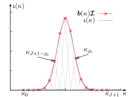
(b)

Figure 1: (a) Mass-attenuation spectrum $\upiota(\kappa)$ obtained by combining the mass attenuation $\kappa(\varepsilon)$ and incident spectrum $\iota(\varepsilon)$, and (b) its B1-spline expansion.

In the following, we review the standard noiseless polychromatic X-ray CT measurement model (Section I-A), existing signal reconstruction approaches from polychromatic measurements (Section I-B), and our mass-attenuation parameterization of this model (Section I-C).

I-A Polychromatic X-ray CT Model

By the exponential law of absorption [8], the fraction $\operatorname{d\!}\mathcal{I}/\mathcal{I}$ of plane wave intensity lost in traversing an infinitesimal thickness $\operatorname{d\!}\ell$ at Cartesian coordinates $(x,y)$ is proportional to $\operatorname{d\!}\ell$:

$$\frac{\operatorname{d\!}\mathcal{I}}{\mathcal{I}}=-\mu(x,y,\varepsilon)\operatorname{d\!}\ell$$ (2)

where $\mu(x,y,\varepsilon)$ is the attenuation. To obtain the intensity decrease along a straight-line path $\ell=\ell(x,y)$ at photon energy $\varepsilon$, integrate (2) along $\ell$: $\mathcal{I}^{\text{out}}(\varepsilon)=\mathcal{I}^{\text{in}}(\varepsilon)\exp\left[-{\int_{\ell}\mu(x,y,\varepsilon)\operatorname{d\!}\ell}\right]$, where $\mathcal{I}^{\text{out}}(\varepsilon)$ and $\mathcal{I}^{\text{in}}(\varepsilon)$ are the emergent and incident X-ray signal energies, respectively, at photon energy $\varepsilon$.

To describe the polychromatic X-ray source, assume that its incident intensity $\mathcal{I}^{\text{in}}$ spreads along photon energy $\varepsilon$ following the density $\iota(\varepsilon)\geq 0$, i.e.,

$$\int\iota(\varepsilon)\operatorname{d\!}\varepsilon=\mathcal{I}^{\text{in}}.$$ (3a)

see Fig. 1(a), which shows a typical density $$\iota(\varepsilon) \ell=\ell(x,y)$$. The noiseless measurement collected by an energy-integrating detector upon traversing a straight line has the superposition-integral form:

$$\mathcal{I}^{\text{out}} = \int\iota(\varepsilon)\exp\left[-{\int_{\ell}\mu(x,y,\varepsilon)\operatorname{d\!}\ell}\right]\operatorname{d\!}\varepsilon$$ (3b)

$$= \int\iota(\varepsilon)\exp\left[-\kappa(\varepsilon)\int_{\ell}\alpha(x,y)\operatorname{d\!}\ell\right]\operatorname{d\!}\varepsilon$$

where we model the attenuation $\mu(x,y,\varepsilon)$ of the inspected object consisting of a single material using the following separable form [9, Sec. 6]:

$$\mu(x,y,\varepsilon)=\kappa(\varepsilon)\alpha(x,y).$$ (4)

Here, $\kappa(\varepsilon)>0$ is the mass-attenuation coefficient of the material, a function of the photon energy $\varepsilon$ (illustrated in Fig. 1(a)) and $\alpha(x,y)\geq 0$ is the density map of the object. For a monochromatic source at photon energy $\varepsilon$, $\ln[\mathcal{I}^{\text{in}}(\varepsilon)/\mathcal{I}^{\text{out}}(\varepsilon)]$ is a linear function of $\alpha(x,y)$, which is a basis for traditional linear reconstruction. However, X-rays generated by vacuum tubes are not monochromatic [10, 5] and we cannot transform the underlying noiseless measurements to a linear model unless we know perfectly the incident energy spectrum $\iota(\varepsilon)$ and mass attenuation of the inspected material $\kappa(\varepsilon)$.

I-B Existing approaches for signal reconstruction from polychromatic X-ray CT measurements

Beam-hardening correction methods can be categorized into pre-filtering, linearization, dual-energy, and post-reconstruction approaches [11]. Reconstruction methods have recently been developed in [12, 13, 14] that aim to optimize nonlinear objective functions based on the underlying physical model; [12, 13] assume known incident polychromatic source spectrum and imaged materials, whereas [14] considers a blind scenario with unknown incident spectrum and imaged materials, but employs an excessive number of parameters and suffers from numerical instability. See also the discussion below and in [15].

I-B1 Linearization

Observe that (3b) is a decreasing function of the line integral $\int_{\ell}\alpha(x,y)\operatorname{d\!}\ell$, which is a key insight behind linearization methods and the water correction approach in [16], popular in the literature and practice, see [9, Sec. 6]. The linearization function has been approximated by exponential or polynomial functions [17, 18]. The linearization functions are obtained by a variety of approaches: [16, 17] assume known spectrum and the materials to simulate the relation between the polychromatic and monochromatic projections; [18] aims to maximize the self-consistency of the projection data to get the correction curve blindly; [11] segments the initial reconstruction to obtain propagation path length of X-ray and then determines the linearization curve.

Indeed, we can derive analytically [if $\kappa(\varepsilon)$ and $\iota(\varepsilon)$ are known] or estimate this monotonic nonlinear function and apply the corresponding inverse function to the noisy measurements. However, such a zero-forcing approach to reconstruction ignores noise and therefore leads to noise enhancement. Due to the difficulty in getting precise linearization function, it has also been reported to introduce a dependency of dimensional measurements on the amount of surrounding material, which is a serious drawback in applications such as CT metrology [1]. The scanning configuration, e.g., X-ray power and prefiltrations, makes choosing accurate linearization function harder. The mass-attenuation parameterization in Fig. 1(a) will allow for improved selection and estimation of the linearization function compared with the existing work. Unlike the traditional linearization, the methods that we aim to develop will estimate the linearization function and account for the noise effects. The zero-forcing linearization schemes could be used to initialize our iterative procedures.

I-B2 Post-reconstruction

The post-reconstruction approach first proposed in [19], uses the segmentation of an initial reconstruction to estimate the traversal length of each X-ray through each material. It assumes known incident X-ray spectrum and attenuation coefficients, as well as that the imaged materials are homogeneous and have constant density, leading to piecewise-constant reconstructed images.

I-B3 Poisson and lognormal statistical measurement models

X-ray photons arriving at a detector can be well modeled using a Poisson process [20, 13], where the energy deposited by each photon follows a distribution that is proportional to the incident energy spectrum. Hence, the measurements collected by photon-counting and energy-integrating detectors are modeled using Poisson and compound-Poisson distributions, respectively [21, 22]. However, the compound-Poisson distribution is complex and does not have a closed-form expression, which motivates introduction of approximations such as Poisson [12] and lognormal [14, 23, 7]. Regardless of the statistical measurement models, most most methods in this category assume known X-ray spectrum and materials (i.e., known mass-attenuation function), with goal to maximize the underlying likelihood function or its regularized version [12, 24]. However, the X-ray spectrum measurements based on the semiconductor detectors are usually distorted by charge trapping, escape events, and other effects [25] and the corresponding correction requires highly collimated beam and special procedures [26, 27]. Knowing the mass-attenuation function can be challenging as well when the inspected material is unknown, or the inspected object is made of compound or mixture with unknown percentage of each constituent.

[14] [14] consider a “blind” scenario for lognormal measurement model with unknown incident spectrum and materials and employ the $K$-means clustering method to initially associate pixels to the materials and then alternate between material segmentation and updating the relative density map, incident X-ray spectrum, and mass attenuation coefficients for each material. The methods in [14] are based on the standard photon-energy parameterization in (3), employ an excessive number of parameters, and suffer from numerical instability [15]. Indeed, alternating iteratively between updating excessive numbers of non-identifiable parameters prevents development of elegant algorithms and achieving robust reconstructions.

I-B4 Dual-energy

In the dual-energy approach by [28] [28], two X-ray scans are performed using two different incident X-ray spectra. This approach is particularly attractive because it does not require image segmentation to separate out different materials and it provides two reconstruction images. Depending on the basis functions chosen for modeling the attenuation coefficients, the two reconstructed images depict two coefficient maps representing photoelectric and Compton scattering interaction [28] or two density maps of the chosen basis materials [29]. The dual-energy approach doubles the scanning time, needs switching scanning energy, and requires the exact knowledge of the spectra.

I-C Mass-attenuation parameterization

We now introduce our parsimonious parameterization of (3b) for signal reconstruction. Since the mass attenuation $\kappa(\varepsilon)$ and incident spectrum density $\iota(\varepsilon)$ are both functions of $\varepsilon$ (see Fig. 1(a)), we combine the variations of these two functions and write (3a) and (3b) as integrals of $\kappa$ rather than $\varepsilon$, with goal to represent our model using two functions $\upiota(\kappa)$ (defined below) and $\alpha(x,y)$ instead of three [$\iota(\varepsilon),\kappa(\varepsilon)$, and $\alpha(x,y)$], see also [6]. Hence, we rewrite (3a) and (3b) as (see Appendix A)

$$\mathcal{I}^{\textup{in}} = \upiota^{\textup{L}}(0)$$ (5a)

$$\mathcal{I}^{\mathrm{out}} = \upiota^{\textup{L}}\left({\int_{\ell}\alpha(x,y)\operatorname{d\!}\ell}\right)$$ (5b)

where $\upiota^{\textup{L}}(s)=\int\upiota(\kappa)\mathrm{e}^{-s\kappa}\operatorname{d\!}\kappa$ is the Laplace transform of the mass-attenuation spectrum $\upiota(\kappa)$, which represents the density of the incident X-ray energy at attenuation $\kappa$; here, $s>0$, in contrast with the traditional Laplace transform where $s$ is generally complex. For invertible $\kappa(\varepsilon)$ with differentiable inverse function $\varepsilon(\kappa)$, $\upiota(\kappa)=\iota(\varepsilon(\kappa))|\varepsilon^{\prime}(\kappa)|\geq 0$, with $\varepsilon^{\prime}(\kappa)=\operatorname{d\!}\varepsilon(\kappa)/\operatorname{d\!}\kappa$, see Appendix A-I. All $\kappa(\varepsilon)$ encountered in practice can be divided into $M+1$ piecewise-continuous segments $\{(e_{m},e_{m+1})\}_{m=0}^{M}$, where $\kappa(\varepsilon)$ in each segment is a differentiable monotonically decreasing function of $\varepsilon$. In this case, (5) holds and the expression for $\upiota(\kappa)$ can be easily extended to this scenario, yielding (see Appendix A-II)

$$\upiota(\kappa)=\sum_{m=0}^{M}1_{(u_{m},v_{m})}(\kappa)\iota(\varepsilon_{m}(\kappa))\left|\varepsilon_{m}^{\prime}(\kappa)\right|$$ (6)

where $1_{(u_{m},v_{m})}(\kappa)$ is an indicator function that takes value 1 when $\kappa\in(u_{m},v_{m})$ and 0 otherwise. The range and inverse of $\kappa(\varepsilon)$ within $(e_{m},e_{m+1})$ are $(u_{m},v_{m})$ and $\varepsilon_{m}(\kappa)$, respectively, with $u_{m}\triangleq\inf_{\varepsilon{\scriptscriptstyle\nearrow}e_{m+1}}\kappa(\varepsilon)<v_{m}\triangleq\sup_{\varepsilon{\scriptscriptstyle\searrow}e_{m}}\kappa(\varepsilon)$.

Observe that the mass-attenuation spectrum $\upiota(\kappa)$ is nonnegative for all $\kappa$:

$$\upiota(\kappa)\geq 0.$$ (7)

Due to its nonnegative support and range, $\upiota^{\textup{L}}(s)$ is a decreasing function of $s$. Here, $s>0$, in contrast with the traditional Laplace transform where $s$ is generally complex. The function $(\upiota^{\textup{L}})^{-1}$ converts the noiseless measurement $\mathcal{I}^{\textup{out}}$ in (5), which is a nonlinear function of the density map $\alpha(x,y)$, into a noiseless linear “measurement” $\int_{\ell}\alpha(x,y)\operatorname{d\!}\ell$. The $(\upiota^{\textup{L}})^{-1}\circ\exp(-\cdot)$ mapping corresponds to the linearization function in [16] [where it was defined through (3b) rather than the mass-attenuation spectrum] and converts $-{\ln\mathcal{I}^{\textup{out}}}$ into a noiseless linear “measurement” $\int_{\ell}\alpha(x,y)\operatorname{d\!}\ell$, see also the discussion in Section I-B1.

The mass-attenuation spectrum depends both on the measurement system (through the incident energy spectrum) and inspected object (through the mass attenuation of the inspected material). In the blind scenario where the inspected material and incident signal spectrum are unknown, the above parameterization allows us to estimate two functions [$\upiota(\kappa)$ and $\alpha(x,y)$] rather than three [$\iota(\varepsilon),\kappa(\varepsilon)$, and $\alpha(x,y)$]. This blind scenario is the focus of this paper.

In Section II, we introduce the density-map and mass-attenuation parameters to be estimated and discuss their identifiability. Section III then presents lognormal and Poisson probabilistic measurement models and biconvexity properties of their negative log-likelihoods (NLLs). Section IV introduces the penalized NLL function that incorporates the parameter constraints and describes the proposed block coordinate-descent algorithm, which alternates between a Nesterov’s proximal-gradient (NPG) step for estimating the density map image and a limited-memory Broyden-Fletcher-Goldfarb-Shanno with box constraints (L-BFGS-B) step for estimating the incident-spectrum parameters. In Section V, we show the performance of the proposed method using simulated and real X-ray CT data. Concluding remarks are given in Section VI.

II Basis-Function Expansion of Mass-Attenuation Spectrum

Upon spatial-domain discretization into $p$ pixels, replace the integral $\int_{\ell}\alpha(x,y)\operatorname{d\!}\ell$ with $\boldsymbol{\phi}^{T}{\boldsymbol{\alpha}}$:

$$\int_{\ell}\alpha(x,y)\operatorname{d\!}\ell\approx\boldsymbol{\phi}^{T}{\boldsymbol{\alpha}}$$ (8)

where ${\boldsymbol{\alpha}}\succeq\boldsymbol{0}$ is a $p\times 1$ vector representing the 2D image that we wish to reconstruct [i.e., discretized $\alpha(x,y)$, see also (7)] and $\boldsymbol{\phi}\succeq\boldsymbol{0}$ is a $p\times 1$ vector of known weights quantifying how much each element of ${\boldsymbol{\alpha}}$ contributes to the X-ray attenuation on the straight-line path $\ell$. An X-ray CT scan consists of hundreds of projections with the beam intensity measured by thousands of detectors for each projection. Denote by $N$ the total number of measurements from all projections collected at the detector array. For the $n$th measurement, define its discretized line integral as $\boldsymbol{\phi}_{n}^{T}{\boldsymbol{\alpha}}$; stacking all $N$ such integrals into a vector yields $\Phi{\boldsymbol{\alpha}}$, where $\Phi=\left[\boldsymbol{\phi}_{1}\,\boldsymbol{\phi}_{2}\dotsb\boldsymbol{\phi}_{N}\right]^{T}\in\mathbb{R}^{N\times p}$ is the projection matrix, also called Radon transform matrix in a parallel-beam X-ray tomographic imaging system. We call the corresponding transformation, $\Phi{\boldsymbol{\alpha}}$, the monochromatic projection of ${\boldsymbol{\alpha}}$.

Approximate $\upiota(\kappa)$ with a linear combination of $J$ ($J\ll N$) basis functions:

$$\upiota(\kappa)={\boldsymbol{b}}(\kappa){\boldsymbol{\mathcal{I}}}$$ (9a)

where

$${\boldsymbol{\mathcal{I}}} \triangleq [\mathcal{I}_{1},\mathcal{I}_{2},\dotsc,\mathcal{I}_{J}]^{T}$$ (9b)

$$\succeq \boldsymbol{0}$$ (9c)

is the $$J\times 1 1\times J$$ vector of corresponding basis-function coefficients and the row vector function

$${\boldsymbol{b}}(\kappa)\triangleq\left[b_{1}(\kappa),b_{2}(\kappa),\dotsc,b_{J}(\kappa)\right]$$ (9d)

consists of B-splines [30] of order one (termed B1 splines, illustrated in Fig. 1(b)); in this case, the decomposition (9a) yields nonnegative elements of the spline coefficients ${\boldsymbol{\mathcal{I}}}$ [based on (7)] and thus allows us to impose the physically meaningful nonnegativity constraint (9c) when estimating ${\boldsymbol{\mathcal{I}}}$. The spline knots are selected from a growing geometric series $\{\kappa_{j}\}_{j=0}^{J+1}$ with $\kappa_{0}>0$,

$$\kappa_{j}=q^{j}\kappa_{0}$$ (10a)

and common ratio

$$q>1$$ (10b)

which yields the B1-spline basis functions:

$$b_{j}(\kappa)=\begin{cases}\displaystyle\frac{\kappa-\kappa_{j-1}}{\kappa_{j}-\kappa_{j-1}},&\kappa_{j-1}\leq\kappa<\kappa_{j}\\ \displaystyle\frac{-\kappa+\kappa_{j+1}}{\kappa_{j+1}-\kappa_{j}},&\kappa_{j}\leq\kappa<\kappa_{j+1}\\ 0,&\text{otherwise}\end{cases}$$ (10c)

where the $$j q (j-1)$$th basis function can be obtained simply by -scaling the th basis function:

$$b_{j}(\kappa)=b_{j+1}\left({q\kappa}\right)$$ (10d)

see also Fig. 1(b).

The geometric-series knots have a wide span from $\kappa_{0}$ to $\kappa_{J+1}$ and compensate larger $\kappa$ (i.e., higher attenuation implying “exponentially” smaller $\mathrm{e}^{-\boldsymbol{\phi}^{T}{\boldsymbol{\alpha}}\kappa_{j}}$ term) with a “geometrically” wider integral range, that results in a more effective approximation of (5). The common ratio $q$ in (10b) determines the resolution of the B1-spline approximation. Here, we select $q$ and $J$ so that the range of $\kappa$ spanning the mass-attenuation spectrum is constant:

$$\frac{\kappa_{J+1}}{\kappa_{0}}=q^{J+1}=\text{const}.$$ (10e)

In summary, the following three tuning constants:

$$(q,\kappa_{0},J)$$ (10f)

define our B1-spline basis functions ${\boldsymbol{b}}(\kappa)$.

Substituting (8) and (9a) into (5) for each of the $N$ measurements yields the following expressions for the incident energy and the $N\times 1$ vector of noiseless measurements:

$$\mathcal{I}^{\textup{in}}({\boldsymbol{\mathcal{I}}}) = {\boldsymbol{b}}^{\textup{L}}(0){\boldsymbol{\mathcal{I}}}$$ (11a)

$${\boldsymbol{\mathcal{I}}}^{\textup{out}}({\boldsymbol{\alpha}},{\boldsymbol{\mathcal{I}}}) = {\boldsymbol{b}}_{\circ}^{\textup{L}}(\Phi{\boldsymbol{\alpha}}){\boldsymbol{\mathcal{I}}}$$ (11b)

where, following the notation in Section I, $\boldsymbol{b}_{\circ}^{\textup{L}}(\boldsymbol{s})=\bigl{(}{\boldsymbol{b}}^{\textup{L}}(s_{n})\bigr{)}_{n=1}^{N}$ is an output basis-function matrix obtained by stacking the $1\times J$ vectors ${\boldsymbol{b}}^{\textup{L}}(s_{n})$ columnwise, and $\boldsymbol{s}=\Phi{\boldsymbol{\alpha}}$ is the monochromatic projection. Since the Laplace transform of (10c) can be computed analytically, ${\boldsymbol{b}}^{\textup{L}}(s)$ has a closed-form expression.

II-A Ambiguity of the density map and mass-attenuation spectrum

We discuss density-map scaling ambiguity under the blind scenario where both the density map ${\boldsymbol{\alpha}}$ and incident spectrum parameters ${\boldsymbol{\mathcal{I}}}$ are unknown. By noting (10d) and the $\kappa$-scaling property of the Laplace transform, $b_{j}\left({q{\kappa}}\right)\stackrel{{\scriptstyle\mathcal{L}}}{{\rightarrow}}\frac{1}{q}b_{j}^{\textup{L}}(s/q)$ for $q>0$, we conclude that selecting $q$ times narrower basis functions $\left[b_{0}(\kappa),b_{1}(\kappa),\dotsc,b_{J-1}(\kappa)\right]$ than those in ${\boldsymbol{b}}(\kappa)$ and $q$ times larger density map and spectral parameters ($q{\boldsymbol{\alpha}}$ and $q{\boldsymbol{\mathcal{I}}}$) yields the same mean output photon energy. Consequently,

$${\boldsymbol{\mathcal{I}}}^{\textup{out}}\bigl{(}{\boldsymbol{\alpha}},[0,\mathcal{I}_{2},\dotsc,\mathcal{I}_{J}]^{T}\bigr{)} = {\boldsymbol{\mathcal{I}}}^{\textup{out}}\bigl{(}q{\boldsymbol{\alpha}},q[\mathcal{I}_{2},\dotsc,\mathcal{I}_{J},0]^{T}\bigr{)}.$$ (12)

Hence, when ${\boldsymbol{\mathcal{I}}}$ has a leading zero, the noiseless signal output remains the same if we shift the elements of ${\boldsymbol{\mathcal{I}}}$ (and correspondingly the mass-attenuation spectrum) to the left, followed by scaling the new ${\boldsymbol{\mathcal{I}}}$ and ${\boldsymbol{\alpha}}$ by $q$. Equivalently, when ${\boldsymbol{\mathcal{I}}}$ has a trailing zero, the noiseless signal output remains the same if we shift the elements of ${\boldsymbol{\mathcal{I}}}$ (and correspondingly the spectrum) to the right and scale the new ${\boldsymbol{\mathcal{I}}}$ and ${\boldsymbol{\alpha}}$ by $1/q$. We refer to this property as the shift ambiguity of the mass-attenuation spectrum, which allows us to rearrange leading or trailing zeros in the mass-attenuation coefficient vector ${\boldsymbol{\mathcal{I}}}$ and position the central nonzero part of ${\boldsymbol{\mathcal{I}}}$.

In Section III, we introduce the lognormal and Poisson measurement models (Sections III-A and III-B) and establish conditions for biconvexity of the corresponding NLLs with respect to the density map and incident-spectrum parameters (Section III-C).

II-B Rank of ${\boldsymbol{b}}_{\circ}^{\textup{L}}(\Phi{\boldsymbol{\alpha}})$ and selection of the number of splines $J$

If ${\boldsymbol{b}}_{\circ}^{\textup{L}}(\Phi{\boldsymbol{\alpha}})$ does not have full column rank, then ${\boldsymbol{\mathcal{I}}}$ is not identifiable even if ${\boldsymbol{\alpha}}$ is known, see (11b). The estimation of ${\boldsymbol{\mathcal{I}}}$ may be numerically unstable if ${\boldsymbol{b}}_{\circ}^{\textup{L}}(\Phi{\boldsymbol{\alpha}})$ is poorly conditioned and has small minimum singular values.

We can think of the noiseless X-ray CT measurements as ${\boldsymbol{b}}^{\textup{L}}(s){\boldsymbol{\mathcal{I}}}$ sampled at different $s=\boldsymbol{\phi}^{T}_{n}{\boldsymbol{\alpha}}\in\bigl{[}0,\max_{n}(\boldsymbol{\phi}^{T}_{n}{\boldsymbol{\alpha}})\bigr{]}$. The following lemma implies that, if we could collect all $s\in[0,a],\,a>0$ (denoted $\boldsymbol{s}$), then the corresponding ${\boldsymbol{b}}_{\circ}^{\textup{L}}(\boldsymbol{s})$ would be a full-rank matrix.

Lemma 1

${\boldsymbol{\mathcal{J}}}=\boldsymbol{0}_{J\times 1}$ is the necessary condition for ${\boldsymbol{b}}^{\textup{L}}(s){\boldsymbol{\mathcal{J}}}=0$ over the range $s\in[0,a]$, where ${\boldsymbol{\mathcal{J}}}\in\mathbb{R}^{J}$ and $a>0$.

Proof:

Use the fact that ${\boldsymbol{b}}^{\textup{L}}(s){\boldsymbol{\mathcal{J}}}$ is analytic with respect to $s$. If ${\boldsymbol{b}}^{\textup{L}}(s){\boldsymbol{\mathcal{J}}}=0$ in the domain $s\in[0,a]$, the $n$th order derivative of ${\boldsymbol{b}}^{\textup{L}}(s){\boldsymbol{\mathcal{J}}}$ with respect to $s$ is zero over this domain for all $n=1,2,\ldots$. Then, according to the Taylor expansion of the whole complex plane at some point in $[0,a]$, ${\boldsymbol{b}}^{\textup{L}}(\cdot){\boldsymbol{\mathcal{J}}}=0$ everywhere. Therefore, ${\boldsymbol{b}}(\kappa){\boldsymbol{\mathcal{J}}}=0$, thus, ${\boldsymbol{\mathcal{J}}}=\boldsymbol{0}$. ∎

If our data collection system can sample over $\bigl{[}0,\max_{n}(\boldsymbol{\phi}^{T}_{n}{\boldsymbol{\alpha}})\bigr{]}$ sufficiently densely, we expect ${\boldsymbol{b}}_{\circ}^{\textup{L}}(\Phi{\boldsymbol{\alpha}})$ to have full column rank.

As the number of splines $J$ increases for fixed support $[\kappa_{0},\kappa_{J+1}]$ [see (10e)], we achieve better resolution of the mass-attenuation spectrum, but ${\boldsymbol{b}}_{\circ}^{\textup{L}}(\Phi{\boldsymbol{\alpha}})$ becomes poorly conditioned with its smallest singular values approaching zero. To estimate this spectrum well, we wish choose a $J$ that provides both good resolution and sufficiently large smallest singular value of ${\boldsymbol{b}}_{\circ}^{\textup{L}}(\Phi{\boldsymbol{\alpha}})$.

Fortunately, we focus on the reconstruction of ${\boldsymbol{\alpha}}$, which is affected by ${\boldsymbol{\mathcal{I}}}$ only through the function ${\boldsymbol{b}}^{\textup{L}}(s){\boldsymbol{\mathcal{I}}}$, and ${\boldsymbol{b}}^{\textup{L}}(s){\boldsymbol{\mathcal{I}}}$ is stable as we increase $J$. Indeed, we observe that, when we choose $J$ that is significantly larger than the rank of ${\boldsymbol{b}}_{\circ}^{\textup{L}}(\Phi{\boldsymbol{\alpha}})$, the estimation of ${\boldsymbol{\alpha}}$ will be good and ${\boldsymbol{b}}_{\circ}^{\textup{L}}(\Phi{\boldsymbol{\alpha}})$ stable, even though the estimation of ${\boldsymbol{\mathcal{I}}}$ is poor due to its non-identifiability. The increase of $J$ will also increase the computational complexity of signal reconstruction under the blind scenario where the mass-attenuation spectrum is unknown.

III Measurement Models and Their Properties

III-A Lognormal measurement model

Consider an $N\times 1$ vector ${\boldsymbol{\mathcal{E}}}$ of energy measurements corrupted by independent lognormal noise and the corresponding NLL function [see (11b)]:

$$\mathcal{L}\left({{\boldsymbol{\alpha}},{\boldsymbol{\mathcal{I}}}}\right)=\frac{1}{2}\bigl{\|}\ln_{\circ}{\boldsymbol{\mathcal{E}}}-\ln_{\circ}{\boldsymbol{\mathcal{I}}}^{\textup{out}}({\boldsymbol{\alpha}},{\boldsymbol{\mathcal{I}}})\bigr{\|}_{2}^{2}.$$ (13)

In the following, we express the NLL (13) as a function of ${\boldsymbol{\alpha}}$ with ${\boldsymbol{\mathcal{I}}}$ fixed (Section III-A1) and vice versa (Section III-A2), and derive conditions for its convexity under the two scenarios. These results will be used to establish the biconvexity conditions for this NLL in Section III-C and to describe our block coordinate-descent estimation algorithm in Section IV.

III-A1 NLL of ${\boldsymbol{\alpha}}$

Recall (9a) and define

$$\upiota_{\circ}^{\textup{L}}(\Phi{\boldsymbol{\alpha}})={\boldsymbol{b}}_{\circ}^{\textup{L}}(\Phi{\boldsymbol{\alpha}}){\boldsymbol{\mathcal{I}}}$$ (14a)

obtained by stacking $$\bigl{\{}\upiota^{\textup{L}}(\boldsymbol{\phi}_{n}^{T}{\boldsymbol{\alpha}})\bigr{\}}_{n=1}^{N} {\boldsymbol{\alpha}} {\boldsymbol{\mathcal{I}}}$$ columnwise. The NLL of for fixed is

$$\mathcal{L}_{\upiota}({\boldsymbol{\alpha}})=\frac{1}{2}\bigl{\|}\ln_{\circ}{\boldsymbol{\mathcal{E}}}-\ln_{\circ}\upiota_{\circ}^{\textup{L}}(\Phi{\boldsymbol{\alpha}})\bigr{\|}_{2}^{2}$$ (14b)

which corresponds to the Gaussian generalized linear model (GLM) for measurements $$\ln_{\circ}({\boldsymbol{\mathcal{E}}}) \Phi (\upiota_{\circ}^{\textup{L}})^{-1}\left({\exp(\cdot)}\right)$$ with design matrix and link function . See [31] for introduction to GLMs.

To establish convexity of the NLL (14b), we enforce monotonicity of the mass-attenuation spectrum $\upiota(\kappa)$ in low- and high-$\kappa$ regions and also assume that the mid-$\kappa$ region has higher spectrum than the low-$\kappa$ region. Note that we do not require here that $\upiota(\kappa)$ satisfies the basis-function expansion (9a); however, the basis-function expansion requirement will be needed to establish the biconvexity of the NLL in (13). Hence, we define the three $\kappa$ regions using the spline parameters (10f) as well as an additional integer constant

$$j_{0}\geq\lceil(J+1)/2\rceil.$$ (15a)

In particular, the low-, mid-, and high-$$\kappa$$ regions are defined as

$$\mathcal{K}_{\text{low}} \triangleq [\kappa_{0},\kappa_{J+1-j_{0}}],$$ K_mid ≜ [κ_J+1-j_0,κ_j_0] K_high ≜ [κ_j_0,κ_J+1]. (15b)

Assumption 1

Assume that the mass-attenuation spectrum satisfies

$$\mathcal{A}=\biggl{\{}\left.{\upiota\mathrel{\mathop{\mathchar 58\relax}}\;[\kappa_{0},\kappa_{J+1}]\rightarrow\mathbb{R}_{+}\,}\right| \upiota \mathcal{K}_{\text{low}} \mathcal{K}_{\text{high}}$$ non-decreasing and non-increasing in and , (16)

$$\text{and $\upiota(\kappa)\geq\upiota(\kappa_{J+1-j_{0}})\,\forall\kappa\in\mathcal{K}_{\text{mid}}$ }\biggr{\}}.$$

If the basis-function expansion (9a) holds, (16) reduces to

$$\mathcal{A}=\biggl{\{}{\boldsymbol{\mathcal{I}}}\in\mathbb{R}_{+}^{J}\,\Big{|}\,\mathcal{I}_{1}\leq\mathcal{I}_{2}\leq\ldots \leq\mathcal{I}_{J+1-j_{0}},\;\mathcal{I}_{j_{0}}\geq\ldots\geq\mathcal{I}_{J-1}\geq\mathcal{I}_{J},\;$$ (17)

$$\text{ and }\mathcal{I}_{j}\geq\mathcal{I}_{J+1-j_{0}},\;\forall j\in[J+1-j_{0},j_{0}]\biggr{\}}$$

see also Fig. 1(b). Here, the monotonic low- and high-$\kappa$ regions each contains $J-j_{0}$ knots in the B1-spline representation, whereas the central region contains $2j_{0}-J$ knots.

In practice, the X-ray spectrum $\iota(\varepsilon)$ starts at a lowest effective energy that can penetrate the object, vanishes at the tube voltage (the highest photon energy) and has a region in the center higher than the two ends, see Fig. 1(a). When the support of $\iota(\varepsilon)$ is free of $K$-edges, the mass attenuation coefficient $\kappa(\varepsilon)$ is monotonic, thus $\upiota(\kappa)$ (as a function of $\kappa$) has the same shape and trends as $\iota(\varepsilon)$ (as a function of $\varepsilon$) and justifies Assumption 1. If a $K$-edge is present within the support of $\iota(\varepsilon)$, it is difficult to infer the shape of $\upiota(\kappa)$. In most cases, Assumption 1 holds.

For the approximation of $\upiota(\kappa)$ using B1-spline basis expansion, as long as $[\kappa_{0},\kappa_{J+1}]$ is sufficiently large to cover the range of $\kappa(\varepsilon)$ with $\varepsilon\in\operatorname*{supp}(\iota(\varepsilon))$, we can always meet Assumption 1 by selecting $j_{0}$ appropriately.

Multiple different $({\boldsymbol{\alpha}},{\boldsymbol{\mathcal{I}}})$ share the same noiseless output ${\boldsymbol{\mathcal{I}}}^{\textup{out}}({\boldsymbol{\alpha}},{\boldsymbol{\mathcal{I}}})$ and thus the same NLL, see Section II-A. In particular, equivalent $({\boldsymbol{\alpha}},{\boldsymbol{\mathcal{I}}})$ can be constructed by left- or right-shifting the mass attenuation spectrum and properly rescaling it and the density map, see (12). Selecting a fixed $j_{0}$ in (15a) can exclude all these equivalent values but the one in which the mass-attenuation spectrum satisfies (16) and where the biconvexity of the NLL can be established.

Lemma 2

Provided that Assumption 1 holds, the lognormal NLL $\mathcal{L}_{\upiota}({\boldsymbol{\alpha}})$ is a convex function of ${\boldsymbol{\alpha}}$ over the following region:

$$\left\{{\boldsymbol{\alpha}}\left|{\,\upiota_{\circ}^{\textup{L}}(\Phi{\boldsymbol{\alpha}})\succeq\mathrm{e}^{-U}{\boldsymbol{\mathcal{E}}},\;{\boldsymbol{\alpha}}\in\mathbb{R}_{+}^{p}}\right.\right\}$$ (18a)

where

$$U\triangleq\frac{2q^{j_{0}}}{(q^{j_{0}}-1)^{2}}.$$ (18b)

Proof:

See Appendix B. ∎

Upon taking the logarithm of both sides and rearranging, the condition in (18a) corresponds to upper-bounding the residuals $\ln\mathcal{E}_{n}-\ln\mathcal{I}_{n}^{\textup{out}}({\boldsymbol{\alpha}},{\boldsymbol{\mathcal{I}}})$ by $U$. The bound $U$ depends only on the common ratio $q$ and constant $j_{0}$ used to describe the constraint on $\upiota(\kappa)$ in Assumption 1. Note that Lemma 2 does not assume a basis-function expansion of the mass-attenuation spectrum, only that it satisfies (16).

If we wish $\upiota(\kappa)$ to cover the same range [i.e., (10e) holds], then reducing $q$ needs to be accompanied by increasing $J$, which also leads to a larger $j_{0}$. Indeed, $q^{j_{0}}$ in $U$ is the ratio of the point where $\upiota(\kappa)$ starts to be monotonically decreasing to the point where the support of $\upiota(\kappa)$ starts, see Fig. 1(b).

III-A2 NLL of ${\boldsymbol{\mathcal{I}}}$

Fix ${\boldsymbol{\alpha}}$ and define

$$A={\boldsymbol{b}}_{\circ}^{\textup{L}}(\Phi{\boldsymbol{\alpha}}).$$ (19a)

The NLL of $${\boldsymbol{\mathcal{I}}} {\boldsymbol{\alpha}} \ln_{\circ}({\boldsymbol{\mathcal{E}}}) A$$ for fixed reduces to a Gaussian GLM for measurements with design matrix and exponential link function:

$$\mathcal{L}_{A}({\boldsymbol{\mathcal{I}}})=\frac{1}{2}\left\lVert\ln_{\circ}{\boldsymbol{\mathcal{E}}}-\ln_{\circ}(A{\boldsymbol{\mathcal{I}}})\right\rVert_{2}^{2}.$$ (19b)

In the following, we first provide the condition for the convexity of $\mathcal{L}_{A}({\boldsymbol{\mathcal{I}}})$:

Lemma 3

The NLL $\mathcal{L}_{A}({\boldsymbol{\mathcal{I}}})$ in (19b) is a convex function of ${\boldsymbol{\mathcal{I}}}$ in the following region:

$$\left\{{\boldsymbol{\mathcal{I}}}\left|{\,A{\boldsymbol{\mathcal{I}}}\preceq\mathrm{e}{\boldsymbol{\mathcal{E}}}}\right.\right\}.$$ (20)

Upon taking the logarithm of both sides and rearranging, the condition in (20) corresponds to $\ln_{\circ}{\boldsymbol{\mathcal{I}}}^{\textup{out}}({\boldsymbol{\alpha}},{\boldsymbol{\mathcal{I}}})-\ln_{\circ}{\boldsymbol{\mathcal{E}}}\preceq\boldsymbol{1}$.

Proof:

Since $\frac{\partial A{\boldsymbol{\mathcal{I}}}}{\partial{\boldsymbol{\mathcal{I}}}^{T}}=A$, we have

$$\frac{\partial\mathcal{L}_{A}({\boldsymbol{\mathcal{I}}})}{\partial{\boldsymbol{\mathcal{I}}}} = A^{T}\operatorname{diag}^{-1}(A{\boldsymbol{\mathcal{I}}})\left[\ln_{\circ}(A{\boldsymbol{\mathcal{I}}})-\ln_{\circ}{\boldsymbol{\mathcal{E}}}\right]$$ (21a)

$$\frac{\partial^{2}\mathcal{L}_{A}({\boldsymbol{\mathcal{I}}})}{\partial{\boldsymbol{\mathcal{I}}}\partial{\boldsymbol{\mathcal{I}}}^{T}} = A^{T}\operatorname{diag}^{-2}(A{\boldsymbol{\mathcal{I}}})\operatorname{diag}\!\left({\boldsymbol{1}-\ln_{\circ}(A{\boldsymbol{\mathcal{I}}})+\ln_{\circ}{\boldsymbol{\mathcal{E}}}}\right)A$$ (21b)

According to (20), $\operatorname{diag}\left({\boldsymbol{1}-\ln_{\circ}(A{\boldsymbol{\mathcal{I}}})+\ln_{\circ}{\boldsymbol{\mathcal{E}}}}\right)\succeq\boldsymbol{0}$, the Hessian (21b) is positive semidefinite, and $\mathcal{L}_{A}({\boldsymbol{\mathcal{I}}})$ is convex. ∎

From the Hessian expression in (21b), we conclude that $\mathcal{L}_{A}({\boldsymbol{\mathcal{I}}})$ in (19b) is strongly convex if the condition (20) holds with strict inequality and design matrix $A$ has full rank.

Combining the convexity results in Lemmas 2 and 3 yields the biconvexity region for the lognormal NLL $\mathcal{L}\left({{\boldsymbol{\alpha}},{\boldsymbol{\mathcal{I}}}}\right)$ in (13), see Section III-C.

III-B Poisson measurement model

For an $N\times 1$ vector ${\boldsymbol{\mathcal{E}}}$ of independent Poisson measurements, the NLL in the form of generalized Kullback-Leibler divergence [32] is [see also (11b)]

$$\mathcal{L}({\boldsymbol{\alpha}},{\boldsymbol{\mathcal{I}}})=\boldsymbol{1}^{T}\left[{\boldsymbol{\mathcal{I}}}^{\textup{out}}({\boldsymbol{\alpha}},{\boldsymbol{\mathcal{I}}})-{\boldsymbol{\mathcal{E}}}\right]-{\boldsymbol{\mathcal{E}}}^{T}\left[\ln_{\circ}{\boldsymbol{\mathcal{I}}}^{\textup{out}}({\boldsymbol{\alpha}},{\boldsymbol{\mathcal{I}}})-\ln_{\circ}{\boldsymbol{\mathcal{E}}}\right].$$ (22)

In the following, we express (22) as a function of ${\boldsymbol{\alpha}}$ with ${\boldsymbol{\mathcal{I}}}$ fixed (Section III-B1) and vice versa (Section III-B2), which will be used to describe our estimation algorithm in Section IV.

III-B1 NLL of ${\boldsymbol{\alpha}}$

Recall (9a) and write the NLL of ${\boldsymbol{\alpha}}$ for fixed ${\boldsymbol{\mathcal{I}}}$ as

$$\mathcal{L}_{\upiota}\left({{\boldsymbol{\alpha}}}\right) = \boldsymbol{1}^{T}\bigl{[}\upiota_{\circ}^{\textup{L}}(\Phi{\boldsymbol{\alpha}})-{\boldsymbol{\mathcal{E}}}\bigr{]}-{\boldsymbol{\mathcal{E}}}^{T}\bigl{[}\ln_{\circ}\upiota_{\circ}^{\textup{L}}(\Phi{\boldsymbol{\alpha}})-\ln_{\circ}{\boldsymbol{\mathcal{E}}}\bigr{]}$$ (23)

which corresponds to the Poisson GLM with design matrix $\Phi$ and link function equal to the inverse of $\upiota^{\textup{L}}(\cdot)$.

Lemma 4

Provided that Assumption 1 holds, the Poisson NLL $\mathcal{L}_{\upiota}({\boldsymbol{\alpha}})$ is a convex function of ${\boldsymbol{\alpha}}$ over the following region:

$$\mathcal{P}=\left\{{\boldsymbol{\alpha}}\left|{\,\upiota_{\circ}^{\textup{L}}(\Phi{\boldsymbol{\alpha}})\succeq(1-V){\boldsymbol{\mathcal{E}}},\;{\boldsymbol{\alpha}}\in\mathbb{R}_{+}^{p}}\right.\right\}$$ (24a)

where

$$V\triangleq\frac{2q^{j_{0}}}{q^{2j_{0}}+1}.$$ (24b)

Proof:

See Appendix B. ∎

Note that the region in (24a) is only sufficient for convexity and that Lemma 4 does not assume a basis-function expansion of the mass-attenuation spectrum, only that it satisfies (16).

Similar to $U$, $1-V$, the lower bound of $\mathcal{I}_{n}^{\textup{out}}({\boldsymbol{\alpha}},{\boldsymbol{\mathcal{I}}})\big{/}\mathcal{E}_{n}$ for all $n$, is also a function of $q^{j_{0}}$, which is determined by the shape of $\upiota(\kappa)$.

III-B2 NLL of ${\boldsymbol{\mathcal{I}}}$

For fixed ${\boldsymbol{\alpha}}$, the NLL of ${\boldsymbol{\mathcal{I}}}$ reduces to [see (19a)]

$$\mathcal{L}_{A}\left({{\boldsymbol{\mathcal{I}}}}\right) = \boldsymbol{1}^{T}\left({A{\boldsymbol{\mathcal{I}}}-{\boldsymbol{\mathcal{E}}}}\right)-{\boldsymbol{\mathcal{E}}}^{T}\left[\ln_{\circ}\left({A{\boldsymbol{\mathcal{I}}}}\right)-\ln_{\circ}{\boldsymbol{\mathcal{E}}}\right]$$ (25)

which corresponds to the Poisson GLM with design matrix $A$ in (19a) and identity link.

Lemma 5

The NLL $\mathcal{L}_{A}({\boldsymbol{\mathcal{I}}})$ in (25) is a convex function of ${\boldsymbol{\mathcal{I}}}$ for all ${\boldsymbol{\mathcal{I}}}\in\mathbb{R}_{+}^{J}$.

Proof:

The gradient and Hessian of the NLL in (25) are

$$\frac{\partial\mathcal{L}_{A}({\boldsymbol{\mathcal{I}}})}{\partial{\boldsymbol{\mathcal{I}}}} = A^{T}\bigl{[}\boldsymbol{1}-\operatorname{diag}^{-1}(A{\boldsymbol{\mathcal{I}}}){\boldsymbol{\mathcal{E}}}\bigr{]}$$ (26a)

$$\frac{\partial^{2}\mathcal{L}_{A}({\boldsymbol{\mathcal{I}}})}{\partial{\boldsymbol{\mathcal{I}}}\partial{\boldsymbol{\mathcal{I}}}^{T}} = A^{T}\operatorname{diag}({\boldsymbol{\mathcal{E}}})\operatorname{diag}^{-2}(A{\boldsymbol{\mathcal{I}}})A$$ (26b)

where the Hessian matrix (26b) is positive semidefinite. Thus, $\mathcal{L}_{A}({\boldsymbol{\mathcal{I}}})$ in (25) is convex on $\mathbb{R}_{+}^{J}$. ∎

From the Hessian expression in (26b), we conclude that $\mathcal{L}_{A}({\boldsymbol{\mathcal{I}}})$ in (25) is strongly convex if the design matrix $A$ has full rank.

Combining the convexity results in Lemmas 4 and 5 yields the biconvexity region for the NLL $\mathcal{L}\left({{\boldsymbol{\alpha}},{\boldsymbol{\mathcal{I}}}}\right)$ in (22), see the following section.

III-C Biconvexity of the NLLs

Theorem 1

Suppose that Assumption 1 in (17) holds. Then,

1. the lognormal NLL function (13) is biconvex [33] with respect to ${\boldsymbol{\alpha}}$ and ${\boldsymbol{\mathcal{I}}}$ in the region

   $$\mathcal{G}=\left\{\left({{\boldsymbol{\alpha}},{\boldsymbol{\mathcal{I}}}}\right)\left|{\,\mathrm{e}^{-U}{\boldsymbol{\mathcal{E}}}\preceq{\boldsymbol{\mathcal{I}}}^{\textup{out}}({\boldsymbol{\alpha}},{\boldsymbol{\mathcal{I}}})\preceq\mathrm{e}{\boldsymbol{\mathcal{E}}},\;{\boldsymbol{\mathcal{I}}}\in\mathcal{A},\;{\boldsymbol{\alpha}}\in\mathbb{R}_{+}^{p}}\right.\right\}$$ (27a)

   which bounds the elements of the residual vector $\ln_{\circ}{\boldsymbol{\mathcal{E}}}-\ln_{\circ}{\boldsymbol{\mathcal{I}}}^{\textup{out}}({\boldsymbol{\alpha}},{\boldsymbol{\mathcal{I}}})$ [whose squared $\ell_{2}$-norm we wish to minimize, see (13)] between $-1$ and $U$, and

2. the Poisson NLL (22) is biconvex with respect to ${\boldsymbol{\alpha}}$ and ${\boldsymbol{\mathcal{I}}}$ in the following set:

   $$\mathcal{P}=\left\{({\boldsymbol{\alpha}},{\boldsymbol{\mathcal{I}}})\left|{\,{\boldsymbol{\mathcal{I}}}^{\textup{out}}({\boldsymbol{\alpha}},{\boldsymbol{\mathcal{I}}})\succeq(1-V){\boldsymbol{\mathcal{E}}},\;{\boldsymbol{\mathcal{I}}}\in\mathcal{A},\;{\boldsymbol{\alpha}}\in\mathbb{R}_{+}^{p}}\right.\right\}$$ (27b)

   which bounds $\mathcal{I}_{n}^{\textup{out}}(\alpha,{\boldsymbol{\mathcal{I}}})\big{/}\mathcal{E}_{n}$ from below by $1-V$ for all $n$, see also (24b).

Proof:

We first show the convexity of the regions defined in (27a) and (27b) with respect to each variable (${\boldsymbol{\alpha}}$ and ${\boldsymbol{\mathcal{I}}}$) with the other fixed. We then show the convexity of the NLL functions (13) and (22) for each variable.

The region $\mathcal{A}$ in (17) is a subspace, thus a convex set. Since ${\boldsymbol{\mathcal{I}}}^{\textup{out}}$ in (11b) is a linear function of ${\boldsymbol{\mathcal{I}}}$, the inequalities comparing ${\boldsymbol{\mathcal{I}}}^{\textup{out}}$ to constants specify a convex set. Therefore, both $\mathcal{G}_{\boldsymbol{\alpha}}\triangleq\{{\boldsymbol{\mathcal{I}}}\left|{\,({\boldsymbol{\alpha}},{\boldsymbol{\mathcal{I}}})\in\mathcal{G}}\right.\}$ and $\mathcal{P}_{\boldsymbol{\alpha}}=\{{\boldsymbol{\mathcal{I}}}\,|\,{({\boldsymbol{\alpha}},{\boldsymbol{\mathcal{I}}})\in\mathcal{P}}\}$ are convex for fixed ${\boldsymbol{\alpha}}\in\mathbb{R}_{+}^{p}$ because both are intersections between the subspace $\mathcal{A}$ and a convex set via ${\boldsymbol{\mathcal{I}}}^{\textup{out}}$. Since $b_{j}(\kappa)\geq 0$, $\bigl{(}b_{j}^{\textup{L}}(s)\bigr{)}_{j=1}^{J}=\int_{\kappa_{j-1}}^{\kappa_{j+1}}b_{j}(\kappa)\mathrm{e}^{-s\kappa}\operatorname{d\!}\kappa$ are decreasing functions of $s$, which, together with the fact that ${\boldsymbol{\mathcal{I}}}\succeq\boldsymbol{0}$, implies that ${\boldsymbol{b}}^{\textup{L}}(\boldsymbol{s}){\boldsymbol{\mathcal{I}}}$ is a decreasing function of $\boldsymbol{s}$. Since the linear transform $\Phi{\boldsymbol{\alpha}}$ preserves convexity, both $\mathcal{G}_{\boldsymbol{\mathcal{I}}}=\{{\boldsymbol{\alpha}}\,|\,({\boldsymbol{\alpha}},{\boldsymbol{\mathcal{I}}})\in\mathcal{G}\}$ and $\mathcal{P}_{\boldsymbol{\mathcal{I}}}=\{{\boldsymbol{\alpha}}\,|\,({\boldsymbol{\alpha}},{\boldsymbol{\mathcal{I}}})\in\mathcal{P}\}$ are convex with respect to ${\boldsymbol{\alpha}}$ for fixed ${\boldsymbol{\mathcal{I}}}\in\mathcal{A}$. Therefore, $\mathcal{G}$ and $\mathcal{P}$ are biconvex with respect to ${\boldsymbol{\mathcal{I}}}$ and ${\boldsymbol{\alpha}}$.

Observe that $\mathcal{G}$ in (27a) is the intersection of the regions specified by Assumption 1 and Lemmas 2 and 3. Thus, within $\mathcal{G}$, the lognormal NLL (13) is a convex function of ${\boldsymbol{\alpha}}$ (with fixed ${\boldsymbol{\mathcal{I}}}$) and ${\boldsymbol{\mathcal{I}}}$ (with fixed ${\boldsymbol{\alpha}}$), respectively. Similarly, $\mathcal{P}$ in (27b) is the intersection of the regions specified by Assumption 1 and Lemmas 4 and 5. Thus, within $\mathcal{P}$, the Poisson NLL (22) is a convex function of ${\boldsymbol{\alpha}}$ (with fixed ${\boldsymbol{\mathcal{I}}}$) and ${\boldsymbol{\mathcal{I}}}$ (with fixed ${\boldsymbol{\alpha}}$), respectively.

By combining the above region and function convexity results, we conclude that (13) and (22) are biconvex within $\mathcal{G}$ and $\mathcal{P}$, respectively. ∎

IV Density-Map and Mass-Attenuation Spectrum Estimation

IV-A Penalized NLL objective function and its properties

Our goal is to compute penalized maximum-likelihood estimates of the density-map and mass-attenuation spectrum parameters $\left({{\boldsymbol{\alpha}},{\boldsymbol{\mathcal{I}}}}\right)$ by solving the following minimization problem:

$$\min_{{\boldsymbol{\alpha}},{\boldsymbol{\mathcal{I}}}}f({\boldsymbol{\alpha}},{\boldsymbol{\mathcal{I}}})$$ (28a)

where

$$f({\boldsymbol{\alpha}},{\boldsymbol{\mathcal{I}}})=\mathcal{L}({\boldsymbol{\alpha}},{\boldsymbol{\mathcal{I}}})+ur({\boldsymbol{\alpha}})+\mathbb{I}_{[0,+\infty)}({\boldsymbol{\mathcal{I}}})$$ (28b)

is the penalized NLL objective function, $u>0$ is a scalar tuning constant, the density-map regularization term $r({\boldsymbol{\alpha}})$ enforces nonnegativity and sparsity of the signal ${\boldsymbol{\alpha}}$ in an appropriate transform [e.g., total-variation (TV) or discrete wavelet transform (DWT) ] domain, and the third summand enforces the nonnegativity of the mass-attenuation spectrum parameters ${\boldsymbol{\mathcal{I}}}$, see (9c). We consider the following two $r({\boldsymbol{\alpha}})$:

$$r({\boldsymbol{\alpha}}) = {\sum}_{i=1}^{p}\sqrt{\sum_{j\in\mathcal{N}_{i}}(\alpha_{i}-\alpha_{j})^{2}}+\mathbb{I}_{[0,+\infty)}({\boldsymbol{\alpha}})$$ (29a)

$$r({\boldsymbol{\alpha}}) = \bigl{\|}\Psi^{T}{\boldsymbol{\alpha}}\bigr{\|}_{1}+\mathbb{I}_{[0,+\infty)}({\boldsymbol{\alpha}})$$ (29b)

where the second summands enforce the nonnegativity of ${\boldsymbol{\alpha}}$. The first summand in (29a) is an isotropic TV-domain sparsity term [34, 35] and $\mathcal{N}_{i}$ is index set of neighbors of the $i$th element of ${\boldsymbol{\alpha}}$, where elements of ${\boldsymbol{\alpha}}$ are arranged to form a 2-dimensional image. Each set $\mathcal{N}_{i}$ consists of two pixels at most, with one on the top and the other on the right of the $i$th pixel, if possible [35]. The first summand in (29b) imposes sparsity of transform-domain density-map coefficients $\Psi^{T}{\boldsymbol{\alpha}}$, where the sparsifying dictionary $\Psi\in\mathbb{R}^{p\times p^{\prime}}$ ($p\leq p^{\prime}$) is assumed to satisfy the orthogonality condition

$$\Psi\Psi^{T}=I_{p}.$$ (30)

In [7], we used the sparsity regularization term (29b) with (30) and the lognormal NLL in (13).

Since both $r({\boldsymbol{\alpha}})$ in (29a) and (29b) are convex for any ${\boldsymbol{\alpha}}$, and $\mathbb{I}_{[0,+\infty)}({\boldsymbol{\mathcal{I}}})$ in (28b) is convex for all ${\boldsymbol{\mathcal{I}}}$, the following holds.

Corollary 1

The objective $f({\boldsymbol{\alpha}},{\boldsymbol{\mathcal{I}}})$ in (28b) is biconvex with respect to ${\boldsymbol{\alpha}}$ and ${\boldsymbol{\mathcal{I}}}$ under the conditions specified by Theorem 1.

Although the NLL may have multiple local minima of the form $q^{n}\widehat{{\boldsymbol{\alpha}}}$ (see Section II-A), those with large $n$ can be eliminated by the regularization penalty. To make it clear, let us first see the impact the ambiguity has on the scaling of the first derivative of the objective function $f({\boldsymbol{\alpha}},{\boldsymbol{\mathcal{I}}})$. From (12), we conclude that $\boldsymbol{z}_{0}=({\boldsymbol{\alpha}},[0,\mathcal{I}_{2},\dotsc,\mathcal{I}_{J}]^{T})$ and $\boldsymbol{z}_{1}=(q{\boldsymbol{\alpha}},q[\mathcal{I}_{2},\dotsc,\mathcal{I}_{J},0]^{T})$ have the same ${\boldsymbol{\mathcal{I}}}^{\textup{out}}({\boldsymbol{\alpha}},{\boldsymbol{\mathcal{I}}})$ and thus the same NLL. The first derivative of $\mathcal{L}({\boldsymbol{\alpha}},{\boldsymbol{\mathcal{I}}})=\mathcal{L}(\boldsymbol{z})$ over ${\boldsymbol{\alpha}}$ at $\boldsymbol{z}_{1}$ is $1/q$ times that at $\boldsymbol{z}_{0}$. Meanwhile, the subgradients of the regularization term at $\boldsymbol{z}_{0}$ and $\boldsymbol{z}_{1}$ with respect to ${\boldsymbol{\alpha}}$ are the same. Hence, with the increase of $n$, the slope of $f({\boldsymbol{\alpha}},{\boldsymbol{\mathcal{I}}})$ is dominated by the penalty term. This is also experimentally confirmed: we see the initialization $q^{n}{\boldsymbol{\alpha}}^{(0)}$ with large $n$ being reduced as the iteration proceeds.

We now establish that the objective function (28b) satisfies the Kurdyka-Łojasiewicz (KL) property [36], which is important for establishing local convergence of block-coordinate schemes in biconvex optimization problems.

Theorem 2 (KL Property)

The objective function $f({\boldsymbol{\alpha}},{\boldsymbol{\mathcal{I}}})$ satisfies the KL property in any compact subset $\mathbb{C}\subseteq\operatorname{dom}(f)$. Here, the NLL $\mathcal{L}({\boldsymbol{\alpha}},{\boldsymbol{\mathcal{I}}})$ is either lognormal or Poisson in (13) or (22), respectively, and the penalty $r({\boldsymbol{\alpha}})$ in (28b) is given in (29a) or (29b).

Proof:

See Appendix C. ∎

Note that the domain of $f$ requires positive measurements such that ${\boldsymbol{\mathcal{I}}}^{\textup{out}}({\boldsymbol{\alpha}},{\boldsymbol{\mathcal{I}}})\succ\boldsymbol{0}$, which excludes the case ${\boldsymbol{\mathcal{I}}}=\boldsymbol{0}$ when no incident X-ray is applied, see also (11b). The compact set assumption keeps the distance between ${\boldsymbol{\mathcal{I}}}$ and $\boldsymbol{0}$ from going to zero.

IV-B Minimization algorithm

The parameters that we wish to estimate are naturally divided into two blocks, ${\boldsymbol{\alpha}}$ and ${\boldsymbol{\mathcal{I}}}$. The large size of ${\boldsymbol{\alpha}}$ prohibits effective second-order methods under the sparsity regularization, whereas ${\boldsymbol{\mathcal{I}}}$ has much smaller size and only nonnegative constraints, thus allowing for more sophisticated solvers, such as the quasi-Newton Broyden-Fletcher-Goldfarb-Shanno (BFGS) approach [37, Sec. 4.3.3.4] that we adopt here. In addition, the scaling difference between ${\boldsymbol{\alpha}}$ and ${\boldsymbol{\mathcal{I}}}$ can be significant so that the joint gradient method for ${\boldsymbol{\alpha}}$ and ${\boldsymbol{\mathcal{I}}}$ together would converge slowly. Therefore, we adopt a block coordinate-descent algorithm to minimize $f({\boldsymbol{\alpha}},{\boldsymbol{\mathcal{I}}})$ in (28b), where the NPG [7] and L-BFGS-B [38] methods are employed to update estimates of the density-map and mass-attenuation spectrum parameters, respectively. The choice of block coordinate-descent optimization is also motivated by the related alternate convex search (ACS) and block coordinate-descent schemes in [33] and [39], respectively, both with convergence guarantees under certain conditions.

We minimize the objective function (28b) by alternatively updating ${\boldsymbol{\alpha}}$ and ${\boldsymbol{\mathcal{I}}}$ using Step 1) and Step 2), respectively, where Iteration $i$ proceeds as follows:

1. (NPG) Set the mass-attenuation spectrum $\upiota(\kappa)={\boldsymbol{b}}(\kappa){\boldsymbol{\mathcal{I}}}^{(i-1)}$, treat it as known, and descend the regularized NLL function $f({\boldsymbol{\alpha}},{\boldsymbol{\mathcal{I}}}^{(i-1)})=\mathcal{L}_{\upiota}({\boldsymbol{\alpha}})+ur({\boldsymbol{\alpha}})$ by applying an NPG step for ${\boldsymbol{\alpha}}$, which yields ${\boldsymbol{\alpha}}^{(i)}$:

   $$\theta^{(i)} = \frac{1}{2}\left[1+\sqrt{1+4\bigl{(}\theta^{(i-1)}\bigr{)}^{2}}\right]$$ (31a)

   $${\overline{{\boldsymbol{\alpha}}}}^{(i)} = {\boldsymbol{\alpha}}^{(i-1)}+\frac{\theta^{(i-1)}-1}{\theta^{(i)}}\bigl{(}{\boldsymbol{\alpha}}^{(i-1)}-{\boldsymbol{\alpha}}^{(i-2)}\bigr{)}$$ (31b)

   $${\boldsymbol{\alpha}}^{(i)} = \arg\min_{\boldsymbol{\alpha}}\frac{1}{2\beta^{(i)}}\bigl{\|}{\boldsymbol{\alpha}}-{\overline{{\boldsymbol{\alpha}}}}^{(i)}+\beta^{(i)}\nabla\mathcal{L}_{\upiota}\bigl{(}{\overline{{\boldsymbol{\alpha}}}}^{(i)}\bigr{)}\bigr{\|}_{2}^{2}+ur({\boldsymbol{\alpha}})$$ (31c)

   where $$\beta^{(i)}>0$$ is an adaptive step size chosen to satisfy the majorization condition:

   $$\mathcal{L}_{\upiota}\bigl{(}{\boldsymbol{\alpha}}^{(i)}\bigr{)}\leq\mathcal{L}_{\upiota}\bigl{(}{\overline{{\boldsymbol{\alpha}}}}^{(i)}\bigr{)} + \bigl{(}{\boldsymbol{\alpha}}^{(i)}-{\overline{{\boldsymbol{\alpha}}}}^{(i)}\bigr{)}^{T}\nabla\mathcal{L}_{\upiota}\bigl{(}{\overline{{\boldsymbol{\alpha}}}}^{(i)}\bigr{)}+\frac{1}{2\beta^{(i)}}\bigl{\|}{\boldsymbol{\alpha}}^{(i)}-{\overline{{\boldsymbol{\alpha}}}}^{(i)}\bigr{\|}_{2}^{2}$$ (31d)

   using a simple adaptation scheme that aims at keeping $\beta^{(i)}$ as large as possible, as long as it satisfies (31d), see Section IV-B3 for details; we also apply the “function restart” [40] to restore the monotonicity and improve convergence of NPG steps.

2. (BFGS) Set the design matrix $A={\boldsymbol{b}}_{\circ}^{\textup{L}}\bigl{(}\Phi{\boldsymbol{\alpha}}^{(i)}\bigr{)}$, treat it as known, and minimize the regularized NLL function $f\bigl{(}{\boldsymbol{\alpha}}^{(i)},{\boldsymbol{\mathcal{I}}}\bigr{)}$ with respect to ${\boldsymbol{\mathcal{I}}}$, i.e.,

   $${\boldsymbol{\mathcal{I}}}^{(i)}=\arg\min_{{\boldsymbol{\mathcal{I}}}\succeq\boldsymbol{0}}\mathcal{L}_{A}({\boldsymbol{\mathcal{I}}})$$ (32)

   using the inner L-BFGS-B iteration, initialized by ${\boldsymbol{\mathcal{I}}}^{(i-1)}$.

We refer to this iteration as the NPG-BFGS algorithm.

The above iteration is the first physical-model based image reconstruction method (in addition to our preliminary work in [6]) for simultaneous blind (assuming unknown incident X-ray spectrum and unknown materials) sparse image reconstruction from polychromatic measurements. In [6], we applied a piecewise-constant (B0 spline) expansion of the mass attenuation spectrum, approximated Laplace integrals with Riemann sums, used a smooth approximation of the nonnegativity penalties in (29) instead of exact, and did not employ signal-sparsity regularization.

The optimization task in (31c) is a proximal step:

$${\boldsymbol{\alpha}}^{(i)} = \operatorname{prox}_{\beta^{(i)}ur}\left({{\overline{{\boldsymbol{\alpha}}}}^{(i)}-\beta^{(i)}\nabla\mathcal{L}_{\upiota}\bigl{(}{\overline{{\boldsymbol{\alpha}}}}^{(i)}\bigr{)}}\right)$$ (33a)

where the proximal operator for scaled (by $$\lambda>0$$) regularization term (29) is defined as [41]

$$\operatorname{prox}_{\lambda r}\left({{\boldsymbol{a}}}\right)=\arg\min_{{\boldsymbol{\alpha}}}\frac{1}{2}\lVert{\boldsymbol{\alpha}}-{\boldsymbol{a}}\rVert_{2}^{2}+\lambda r({\boldsymbol{\alpha}}).$$ (33b)

If we do not apply the Nesterov’s acceleration (31a)–(31b) and use only the proximal-gradient (PG) step (31c) to update the density-map iterates ${\boldsymbol{\alpha}}$, i.e.,

$${\overline{{\boldsymbol{\alpha}}}}^{(i)}={\boldsymbol{\alpha}}^{(i-1)}$$ (34)

then the corresponding iteration is the PG-BFGS algorithm, see also the numerical examples and Fig. 8(b). We show that our PG-BFGS algorithm is monotonic (Section IV-B3) and converges to one of the critical points of the objective $f({\boldsymbol{\alpha}},{\boldsymbol{\mathcal{I}}})$ (Section IV-B5). Unfortunately, such theoretical convergence properties do not carry over to NPG-BFGS iteration, yet this iteration empirically outperforms the PG-BFGS method, see Section V.

If the mass-attenuation spectrum $\upiota(\kappa)$ is known and we iterate Step 1) only to estimate the density map ${\boldsymbol{\alpha}}$, we refer to this iteration as the NPG algorithm for ${\boldsymbol{\alpha}}$.

Step 1) employs only one NPG step, where an inner iteration is needed to compute the proximal step (31c), whereas Step 2) employs a full L-BFGS-B iteration. Hence, both Step 1) and Step 2) require inner iterations. To solve (33b) for the two regularizations, we adopt

• TV-based denoising method in [35, Sec. IV] for the TV regularization (29a) and

• the alternating direction method of multipliers (ADMM) method for the DWT-based regularization (29b), described in the following section.

IV-B1 Proximal Mapping using ADMM for DWT-based regularization

We now present an ADMM scheme for computing the proximal operator in (33b) for the DWT-based regularization (29b) (see [42, Appendix LABEL:nesterovreport-app:ADMM]):

$${\boldsymbol{\alpha}}^{(k+1)} = \frac{1}{1+\rho}\left({{\boldsymbol{a}}+\rho\Psi\left({\boldsymbol{s}^{(k)}+\boldsymbol{\upsilon}^{(k)}}\right)}\right)_{+}$$ (35a)

$$\boldsymbol{s}^{(k+1)} = \operatorname{\mathcal{T}}_{\frac{\lambda}{\rho}}\left({\Psi^{T}{\boldsymbol{\alpha}}^{(k+1)}-\boldsymbol{\upsilon}^{(k)}}\right)$$ (35b)

$$\boldsymbol{\upsilon}^{(k+1)} = \boldsymbol{\upsilon}^{(k)}+\boldsymbol{s}^{(k+1)}-\Psi^{T}{\boldsymbol{\alpha}}^{(k+1)}$$ (35c)

where $k$ is the inner-iteration index and $\rho>0$ is a step-size parameter, usually set to 1 [43, Sec. 11]. We obtain (35) by decomposing the proximal objective function (33b) into the sum of $\frac{1}{2}\left\lVert{\boldsymbol{\alpha}}-{\boldsymbol{a}}\right\rVert_{2}^{2}+\mathbb{I}_{[0,+\infty)}({\boldsymbol{\alpha}})$ and $\lambda\lVert\Psi^{T}{\boldsymbol{\alpha}}\rVert_{1}$. The above algorithm is initialized by

$$\boldsymbol{s}^{(0)}=\Psi^{T}{\boldsymbol{a}}\qquad\text{and}\qquad\boldsymbol{\upsilon}^{(0)}=\boldsymbol{0}_{p^{\prime}\times 1}$$ (36)

which is equivalent to projecting the noisy signal ${\boldsymbol{a}}$ onto the nonnegative signal space ${\boldsymbol{\alpha}}^{(1)}=({\boldsymbol{a}})_{+}$. Note that the signal estimate $\bigl{(}\Psi\boldsymbol{s}^{(j)}\bigr{)}_{+}$ is within the signal space and yields finite objective function $\frac{1}{2}\lVert{\boldsymbol{\alpha}}-{\boldsymbol{a}}\rVert_{2}^{2}+\lambda r({\boldsymbol{\alpha}})$ that we wish to minimize; we use it to obtain the final signal estimate upon convergence of the ADMM iteration.

In the following, we describe the convergence criteria for the outer and inner iterations (Section IV-B2), adaptive step-size selection (Section IV-B3), algorithm initialization (Section IV-B4), and convergence analysis (Section IV-B5).

IV-B2 Convergence criteria

Define the measures of change of the density map ${\boldsymbol{\alpha}}$ and the NLL

$$\delta^{(i)} = \bigl{\lVert}{\boldsymbol{\alpha}}^{(i)}-{\boldsymbol{\alpha}}^{(i-1)}\bigr{\rVert}_{2}$$ (37a)

$$\delta_{\mathcal{L}}^{(i)} = \left\lvert\mathcal{L}\bigl{(}{\boldsymbol{\alpha}}^{(i)},{\boldsymbol{\mathcal{I}}}^{(i-1)}\bigr{)}-\mathcal{L}\bigl{(}{\boldsymbol{\alpha}}^{(i-1)},{\boldsymbol{\mathcal{I}}}^{(i-1)}\bigr{)}\right\rvert$$ (37b)

upon completion of Step 1) in Iteration $i$. We run the outer iteration between Step 1) and Step 2) until the relative distance of consecutive iterates of the density map ${\boldsymbol{\alpha}}$ does not change significantly:

$$\delta^{(i)}<\epsilon\bigl{\lVert}{\boldsymbol{\alpha}}^{(i)}\bigr{\rVert}_{2}$$ (38)

where $\epsilon>0$ is the convergence threshold.

Proximal step (31c). The convergence criteria for the inner TV-denoising and ADMM iterations used to solve (31c) in Iteration $i$ are based on the relative change $\delta^{(i-1)}$:

$$\bigl{\|}{\boldsymbol{\alpha}}^{(i,k)}-{\boldsymbol{\alpha}}^{(i,k-1)}\bigr{\|}_{2} < \eta_{\boldsymbol{\alpha}}\delta^{(i-1)}$$ (39a)

$$\max\left\{\bigl{\|}\boldsymbol{s}^{(i,k)}-\Psi^{T}{\boldsymbol{\alpha}}^{(i,k)}\bigr{\|}_{2},\bigl{\|}\boldsymbol{s}^{(i,k)}-\boldsymbol{s}^{(i,k-1)}\bigr{\|}_{2}\right\} < \eta_{\boldsymbol{\alpha}}\delta^{(i-1)}$$ (39b)

where $k$ are the inner-iteration indices and the convergence tuning constant $\eta_{\boldsymbol{\alpha}}\in(0,1)$ is chosen to trade off the accuracy and speed of the inner iterations and provide sufficiently accurate solutions to (31c). Note that $\boldsymbol{s}^{(i,k)}$ in (39b) is the dual variable in ADMM that converges to $\Psi^{T}{\boldsymbol{\alpha}}^{(i,k)}$, and the criterion is on both the primal residual $\bigl{\|}\boldsymbol{s}^{(i,k)}-\Psi^{T}{\boldsymbol{\alpha}}^{(i,k)}\bigr{\|}_{2}$ and the dual residual $\bigl{\|}\boldsymbol{s}^{(i,k)}-\boldsymbol{s}^{(i,k-1)}\bigr{\|}_{2}$ [43, Sec. 3.3].

BFGS step (32). For Step 2) in Iteration $i$, we set the convergence criterion as

$$\bigl{|}\mathcal{L}_{A}({\boldsymbol{\mathcal{I}}}^{(i,k)})-\mathcal{L}_{A}({\boldsymbol{\mathcal{I}}}^{(i,k-1)})\bigr{|}<\eta_{{\boldsymbol{\mathcal{I}}}}\delta^{(i)}_{\mathcal{L}}$$ (40)

where the tuning constant $\eta_{{\boldsymbol{\mathcal{I}}}}\in(0,1)$ trades off the accuracy and speed of the estimation of ${\boldsymbol{\mathcal{I}}}$. Since our main goal is to estimate the density map ${\boldsymbol{\alpha}}$, the benefit to Step 1) provided by Step 2) through the minimization of $\mathcal{L}_{A}({\boldsymbol{\mathcal{I}}})$ in (32) is more important than the reconstruction of ${\boldsymbol{\mathcal{I}}}$ itself; furthermore, the estimation of ${\boldsymbol{\mathcal{I}}}$ is sensitive to the rank of $A$. Hence, we select $\delta_{\mathcal{L}}^{(i)}$ as a convergence metric for the inner iteration for ${\boldsymbol{\mathcal{I}}}$ in Step 2) of Iteration $i$.

We safeguard both the proximal and BFGS steps by setting the maximum number of iteration limit $n_{\text{sub}}$. In summary, the outer and inner convergence tuning constants are $(\epsilon,\eta_{\boldsymbol{\alpha}},\eta_{\boldsymbol{\mathcal{I}}},n_{\text{sub}})$. The default values of these tuning constants are

$$\left({\epsilon,\eta_{\boldsymbol{\alpha}},\eta_{\boldsymbol{\mathcal{I}}},n_{\text{sub}}}\right)=\left({10^{-6},10^{-3},10^{-2},20}\right)$$ (41)

adopted in all numerical examples in this paper.

IV-B3 Adaptive step-size selection in Step 1)

We adopt an adaptive step size selection strategy to accommodate the scenarios when the local Lipschitz constant varies as the algorithm evolves.

We select the step size $\beta^{(i)}$ to satisfy the majorization condition (31d) using the following adaptation scheme [42, 44]:

1. In Iteration $i$: if there has been no step size reductions for $\mathbbm{n}$ consecutive iterations, i.e., $\beta^{(i-1)}=\beta^{(i-2)}=\dotsb=\beta^{(i-\mathbbm{n}-1)}$, start with a larger step size $\beta^{(i)}=\beta^{(i-1)}/\xi$, where $\xi\in(0,1)$ is a step-size adaptation parameter; otherwise start with $\beta^{(i)}=\beta^{(i-1)}$;

2. Backtrack using the same multiplicative scaling constant $\xi$, with goal to find the largest $\beta^{(i)}$ that satisfies (31d).

We select the initial step size $\beta^{(0)}$ using the Barzilai-Borwein method [45].

IV-B4 Initialization

Initialize the density-map and mass-attenuation coefficient vector iterates as

$${\boldsymbol{\alpha}}^{(0)} = {\boldsymbol{\alpha}}^{(-1)}=\widehat{{\boldsymbol{\alpha}}}_{\text{FBP}},\qquad\theta^{(0)}=0$$ (42a)

$${\boldsymbol{\mathcal{I}}}^{(0)} = \frac{\max_{n}\mathcal{E}_{n}}{b_{\lceil(J+1)/2\rceil}^{\textup{L}}(0)}\boldsymbol{e}_{\lceil(J+1)/2\rceil}$$ (42b)

where $\widehat{{\boldsymbol{\alpha}}}_{\text{FBP}}$ is the standard FBP reconstruction [10, Ch. 3], [5, Sec. 3.5]. We select the initial step size $\beta^{(0)}$ using the Barzilai-Borwein method [45]. Plugging the initialization (42b) into (11b) yields $\mathcal{I}^{\textup{in}}\bigl{(}{\boldsymbol{\mathcal{I}}}^{(0)}\bigr{)}=\max_{n}\mathcal{E}_{n}$ and the initial estimate $\bigl{(}{\boldsymbol{\alpha}}^{(0)},{\boldsymbol{\mathcal{I}}}^{(0)}\bigr{)}$ corresponds approximately to a monochromatic X-ray model; more precisely, it is a polychromatic X-ray model with a narrow mass attenuation spectrum proportional to $b_{\lceil(J+1)/2\rceil}(\kappa)$. It is also desirable to have the main lobe of the estimated spectrum at the center, which is why the nonzero element of ${\boldsymbol{\mathcal{I}}}^{(0)}$ is placed in the middle position.

IV-B5 Convergence Analysis of PG-BFGS Iteration

We analyze the convergence of the PG-BFGS iteration using arguments similar to those in [39]. Although NPG-BFGS converges faster than PG-BFGS empirically, it is not easy to analyze its convergence due to NPG’s Nesterov’s acceleration step and adaptive step size. In this section, we denote the sequence of PG-BFGS iterates by $\bigl{\{}\bigl{(}{\boldsymbol{\alpha}}^{(i)},{\boldsymbol{\mathcal{I}}}^{(i)}\bigr{)}\bigr{\}}_{i=0}^{\infty}$.

The following lemma establishes the monotonicity of the PG-BFGS iteration for step sizes $\beta^{(i)}$ that satisfy the majorization condition, which includes the above step-size selection as well.

Lemma 6

For a sequence $\bigl{\{}\bigl{(}{\boldsymbol{\alpha}}^{(i)},{\boldsymbol{\mathcal{I}}}^{(i)}\bigr{)}\bigr{\}}_{i=0}^{\infty}$ of PG-BFGS iterates with step size $\beta^{(i)}$ satisfying the majorization condition (31d), the objective function $f({\boldsymbol{\alpha}},{\boldsymbol{\mathcal{I}}})$ in (28b) is monotonically non-increasing:

$$f\bigl{(}{\boldsymbol{\alpha}}^{(i)},{\boldsymbol{\mathcal{I}}}^{(i)}\bigr{)}\leq f\bigl{(}{\boldsymbol{\alpha}}^{(i-1)},{\boldsymbol{\mathcal{I}}}^{(i-1)}\bigr{)}$$ (43)

for all $i$ under the conditions specified by Theorem 1.

Proof:

Due to Theorem 1, $f({\boldsymbol{\alpha}},{\boldsymbol{\mathcal{I}}}^{(i-1)})$ is a convex function of ${\boldsymbol{\alpha}}$; hence, we can apply [46, Lemma 2.3] to obtain

$$f\bigl{(}{\boldsymbol{\alpha}},{\boldsymbol{\mathcal{I}}}^{(i-1)}\bigr{)}-f\bigl{(}{\boldsymbol{\alpha}}^{(i)},{\boldsymbol{\mathcal{I}}}^{(i-1)}\bigr{)}\geq\frac{1}{2\beta^{(i)}}\left[\bigl{\|}{\boldsymbol{\alpha}}^{(i)}-{\overline{{\boldsymbol{\alpha}}}}^{(i)}\bigr{\|}_{2}^{2}+2({\overline{{\boldsymbol{\alpha}}}}^{(i)}-{\boldsymbol{\alpha}})^{T}({\boldsymbol{\alpha}}^{(i)}-{\overline{{\boldsymbol{\alpha}}}}^{(i)})\right]$$ (44a)

for any $${\boldsymbol{\alpha}} {\boldsymbol{\alpha}}={\boldsymbol{\alpha}}^{(i-1)}$$, as long as (31d) is satisfied. In the PG-BFGS iteration, the momentum term in (31b) is zero, i.e., (34) holds. Plug in (34) and into (44a):

$$f\bigl{(}{\boldsymbol{\alpha}}^{(i-1)},{\boldsymbol{\mathcal{I}}}^{(i-1)}\bigr{)}-f\bigl{(}{\boldsymbol{\alpha}}^{(i)},{\boldsymbol{\mathcal{I}}}^{(i-1)}\bigr{)}\geq\frac{1}{2\beta^{(i)}}\bigl{\|}{\boldsymbol{\alpha}}^{(i)}-{\boldsymbol{\alpha}}^{(i-1)}\bigr{\|}_{2}^{2}\geq 0$$ (44b)

and (43) follows by using the fact $f\bigl{(}{\boldsymbol{\alpha}}^{(i)},{\boldsymbol{\mathcal{I}}}^{(i-1)}\bigr{)}\geq f\bigl{(}{\boldsymbol{\alpha}}^{(i)},{\boldsymbol{\mathcal{I}}}^{(i)}\bigr{)}$, see Step 2). ∎

Unfortunately, the monotonicity does not carry over when Nesterov acceleration is employed and the momentum term is not zero; this case requires further adjustments such as restart, as described in Step 1).

Since our $f({\boldsymbol{\alpha}},{\boldsymbol{\mathcal{I}}})$ are lower bounded [which is easy to argue, see Appendix C], the sequence $f({\boldsymbol{\alpha}}^{(i)},{\boldsymbol{\mathcal{I}}}^{(i)})$ converges. It is also easy to conclude that the sequence $a_{i}\triangleq\frac{1}{\beta^{(i)}}\bigl{\|}{\boldsymbol{\alpha}}^{(i)}-{\boldsymbol{\alpha}}^{(i-1)}\bigr{\|}_{2}^{2}$ is Cauchy by showing $\sum_{i=0}^{\infty}a_{i}<+\infty$; thus ${\boldsymbol{\alpha}}^{(i)}$ converges to a critical point (also called stationary point) ${\boldsymbol{\alpha}}^{\star}$ [36, Lemma 2.2]. A better result $\sum_{i=0}^{\infty}\bigl{\|}{\boldsymbol{\alpha}}^{(i)}-{\boldsymbol{\alpha}}^{(i+1)}\bigr{\|}_{2}<+\infty$ [39] can be established if we can show that $f({\boldsymbol{\alpha}},{\boldsymbol{\mathcal{I}}})$ satisfies the KL property [36], which regularizes the (sub)gradient of a function through its value at certain point or the whole domain and also ensures the steepness of the function around the optimum so that the length of the gradient trajectory is bounded. The KL property has been first used in [36] to establish the critical-point convergence for an alternating proximal-minimization method, which is then extended by [39] to the more general block coordinate-descent method.

Now, we can make the following claim on the convergence of PG-BFGS iteration.

Theorem 3

Consider the sequence $\bigl{\{}\bigl{(}{\boldsymbol{\alpha}}^{(i)},{\boldsymbol{\mathcal{I}}}^{(i)}\bigr{)}\bigr{\}}_{i=0}^{\infty}$ of PG-BFGS iterates, with step size $\beta^{(i)}$ satisfying the majorization condition (31d). Assume that

1. there exist positive $\beta_{+}>\beta_{-}>0$ such that $\beta^{(i)}\in[\beta_{-},\beta_{+}]$ for all $i$,

2. $\mathcal{L}({\boldsymbol{\alpha}},{\boldsymbol{\mathcal{I}}})$ is a strong convex function of ${\boldsymbol{\mathcal{I}}}$, and

3. the first derivative of $f({\boldsymbol{\alpha}},{\boldsymbol{\mathcal{I}}})$ over $({\boldsymbol{\alpha}},{\boldsymbol{\mathcal{I}}})$ is Lipschitz continuous

and that the conditions of Theorem 1 hold, ensuring the biconvexity of $f$. Then, $({\boldsymbol{\alpha}}^{(i)},{\boldsymbol{\mathcal{I}}}^{(i)})$ converges to one of the critical points $({\boldsymbol{\alpha}}^{\star},{\boldsymbol{\mathcal{I}}}^{\star})$ of $f({\boldsymbol{\alpha}},{\boldsymbol{\mathcal{I}}})$ and

$$\sum_{i=1}^{\infty}\bigl{\|}{\boldsymbol{\alpha}}^{(i+1)}-{\boldsymbol{\alpha}}^{(i)}\bigr{\|}_{2}<+\infty, \sum_{i=1}^{\infty}\bigl{\|}{\boldsymbol{\mathcal{I}}}^{(i+1)}-{\boldsymbol{\mathcal{I}}}^{(i)}\bigr{\|}_{2}<+\infty$$ (45)

Proof:

See Appendix C. ∎

The conditions for strong convexity of $\mathcal{L}\left({{\boldsymbol{\alpha}},{\boldsymbol{\mathcal{I}}}}\right)$ as a function of ${\boldsymbol{\alpha}}$ are discussed in Sections III-A2 and III-B2, see also Section II-B. The KL property can provide guarantees on the convergence rate under additional assumptions, see [36, Theorem 3.4]. The convergence properties of NPG-BFGS are of great interest because NPG-BFGS converges faster than PG-BFGS; establishing these properties is left as future work.

V Numerical Examples

We now evaluate our proposed algorithm by both numerical simulations and real data reconstructions. Here, we focus on the Poisson measurement model only and refer to [7] for the lognormal case.

We construct the fan-beam X-ray projection transform matrix $\Phi$ and its adjoint operator $\Phi^{T}$ directly on GPU with full circular mask [47], and the multi-thread version on CPU is also available; see https://github.com/isucsp/imgRecSrc.

Before applying the reconstruction algorithms, the measurements $${\boldsymbol{\mathcal{E}}} \max_{n}\mathcal{E}_{n}=1$$ are normalized by division of their maximum such that , which stabilizes the magnitude of NLL by scaling it with a constant, see (22). We set the B1-spline tuning constants (10f) to satisfy [see also (10e)]

$$q^{J}=10^{3}, \kappa_{\lceil 0.5(J+1)\rceil}=1, J=30$$ (46a)

which ensure sufficient coverage (three orders of magnitude) and resolution (30 basis functions) of the basis-function representation of the mass-attenuation spectrum and centering its support around 1. We set the convergence and adaptive step-size tuning constants for the NPG-BFGS method as

$$(\epsilon,\eta_{\boldsymbol{\alpha}},\eta_{\boldsymbol{\mathcal{I}}},n_{\text{sub}})=\bigl{(}10^{-6},10^{-3},10^{-2},20\bigr{)}, (n,\xi)=(4,0.5)$$ (46b)

limit the number of outer iterations to $$4000$$ at most.

V-A Reconstruction from simulated Poisson measurements

(a)

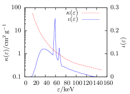
(b)

Figure 2: (a) Density-map image and (b) mass attenuation and incident X-ray spectrum as functions of the photon energy $\varepsilon$.

Consider reconstruction of the $512\text{\times}512$ image in Fig. 2(a) of an iron object with density map ${\boldsymbol{\alpha}}_{\text{true}}$. We generated a fan-beam polychromatic sinogram, with distance from X-ray source to the rotation center equal to $2000$ times the pixel size, using the interpolated mass attenuation $\kappa(\varepsilon)$ of iron [48] and incident spectrum $\iota(\varepsilon)$ from tungsten anode X-ray tubes at $140\text{\,}\text{\mathrm{ k }\mathrm{ eV }}$ with $5\text{\,}\mathrm{\char 37\relax}$ relative voltage ripple [49], see Fig. 2(b). The mass-attenuation spectrum $\upiota(\kappa)$ is constructed by combining $\kappa(\varepsilon)$ and $\iota(\varepsilon)$, see [6] and [7, Fig. LABEL:qnde14-fig:triRelate]. Our simulated approximation of the noiseless measurements uses $130$ equi-spaced discretization points over the range $20\text{\,}\text{\mathrm{ k }\mathrm{ eV }}140\text{\,}\text{\mathrm{ k }\mathrm{ eV }}$. We simulated independent Poisson measurements $\left({\mathcal{E}_{n}}\right)_{n=1}^{N}$ with means $\left({\operatorname{E}\mathcal{E}_{n}}\right)_{n=1}^{N}={\boldsymbol{\mathcal{I}}}^{\textup{out}}({\boldsymbol{\alpha}},{\boldsymbol{\mathcal{I}}})$. We mimic real X-ray CT system calibration by scaling the projection matrix $\Phi$ and the spectrum $\iota(\varepsilon)$ so that the maximum and minimum of the noiseless measurements $\left({\operatorname{E}\mathcal{E}_{n}}\right)_{n=1}^{N}$ are $2^{16}$ and $20$, respectively. Here, the scales of $\Phi$ and $\iota(\varepsilon)$ correspond to the real size that each image pixel represents and the current of the electrons hitting the tungsten anode as well as the overall scanning time.

Our goal here is to reconstruct a density map of size $512\text{\times}512$ by the measurements from an energy-integrating detector array of size 512 for each projection.

Since the true density map is known, we adopt relative square error (RSE) as the main metric to assess the performance of the compared algorithms:

$$\operatorname{RSE}\{\widehat{{\boldsymbol{\alpha}}}\}=1-\left({\frac{\widehat{{\boldsymbol{\alpha}}}^{T}{\boldsymbol{\alpha}}_{\text{true}}}{{\|\widehat{{\boldsymbol{\alpha}}}\|_{2}\|{\boldsymbol{\alpha}}_{\text{true}}\|_{2}}}}\right)^{2}$$ (47)

where ${\boldsymbol{\alpha}}_{\text{true}}$ and $\widehat{{\boldsymbol{\alpha}}}$ are the true and reconstructed signals, respectively. Note that (47) is invariant to scaling $\widehat{{\boldsymbol{\alpha}}}$ by a nonzero constant, which is needed because the magnitude level of ${\boldsymbol{\alpha}}$ is not identifiable due to the ambiguity of the density map and mass attenuation spectrum (see also Section. II-A).

We compare

• the traditional FBP method without [10, Ch. 3] and with linearization [16], i.e., based on the ‘data’

  $$\boldsymbol{y}=-{\ln_{\circ}({\boldsymbol{\mathcal{E}}})}$$ (without linearization) (48a)

  $$\boldsymbol{y}=\bigl{(}\upiota^{\textup{L}}\bigr{)}_{\circ}^{-1}({\boldsymbol{\mathcal{E}}})$$ (with linearization) (48b)

  respectively,

• linearized basis pursuit denoising (BPDN) in which we apply the NPG approach to solve the BPDN problem [35]:

  $$\min_{{\boldsymbol{\alpha}}}\frac{1}{2}\|\boldsymbol{y}-\Phi{\boldsymbol{\alpha}}\|_{2}^{2}+u^{\prime}r({\boldsymbol{\alpha}})$$ (49)

  where $\boldsymbol{y}$ are the linearized measurements by (48b) and the penalty $r({\boldsymbol{\alpha}})$ has been defined in (29).

• our

  • NPG-BFGS alternating descent method,

  • NPG for known mass attenuation spectrum $\upiota(\kappa)$.

  with the Matlab implementation available at https://github.com/isucsp/imgRecSrc.

For all methods that use sparsity and nonnegativity regularization (NPG-BFGS, NPG, and linearized BPDN) the regularization constants $u$ and $u^{\prime}$ have been tuned manually for best RSE performance. All iterative algorithms employ the convergence criterion (38) with threshold $\epsilon=${10}^{-6}$$ and the maximum number of iterations set to $4000$. We initialize iterative reconstruction schemes with or without linearization using the corresponding FBP reconstructions.

Here, the non-blind linearized FBP, NPG, and linearized BPDN methods assume known $\upiota(\kappa)$ [i.e., known incident spectrum of the X-ray machine and mass attenuation (material)], which we computed using (9a) with ${\boldsymbol{\mathcal{I}}}$ equal to the exact sampled $\upiota(\kappa)$ and $J=100$ spline basis functions spanning three orders of magnitude. The FBP and NPG-BFGS methods are blind and do not assume knowledge of $\upiota(\kappa)$; FBP ignores the polychromatic source effects whereas NPG-BFGS corrects blindly for these effects.

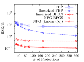
Figure 3: Average RSEs as functions of the number of projections.

Fig. 3 shows the average RSEs (over 5 Poisson noise realizations) of different methods as functions of the number of fan-beam projections in the range from $0\text{\,}\mathrm{\SIUnitSymbolDegree}359\text{\,}\mathrm{\SIUnitSymbolDegree}$. RSEs of the methods that do not assume knowledge of the mass attenuation spectrum $\upiota(\kappa)$ are shown using solid lines whereas dashed lines represent methods that assume known $\upiota(\kappa)$ [i.e., known incident spectrum of the X-ray machine and mass attenuation (material)]. Blue color presents methods that do not employ regularization; red color presents methods that employ regularization.

FBP ignores the polychromatic nature of the measurements and consequently performs poorly and does not improve as the number of projections increases. Linearized FBP, which assumes perfect knowledge of the mass attenuation spectrum, performs much better than FBP as shown in Fig. 3. Thanks to the nonnegativity and sparsity that it imposes, linearized BPDN achieves up to 20 times smaller RSE than linearized FBP. However, the linearization process employed by linearized BPDN enhances the noise (due to the zero-forcing nature of linearization) and does not account for the Poisson measurements model. Note that linearized BPDN exhibits a noise floor as the number of projections increases.

As expected, NPG is slightly better than NPG-BFGS because it assumes knowledge of $\upiota(\kappa)$. NPG and NPG-BFGS attain RSEs that are $24\text{\,}\mathrm{\char 37\relax}37\text{\,}\mathrm{\char 37\relax}$ that of linearized BPDN, which can be attributed to optimal statistical processing of the proposed methods, in contrast with suboptimal linearization. RSEs of NPG and NPG-BFGS reach a noise floor when the number of projections increases beyond 180.

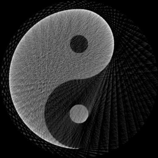
(a) FBP

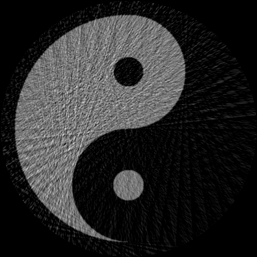
(b) linearized FBP

(c) linearized BPDN

(d) NPG-BFGS

(e) NPG (known $\upiota(\kappa)$)

Figure 4: Reconstructions from $60$ projections.

Fig. 4 shows the reconstructions from 60 equi-spaced fan-beam projections with spacing $6^{\circ}$. The FBP reconstruction in Fig. 4(a) is corrupted by both aliasing and beam-hardening (cupping and streaking) artifacts. The intensity is high along the outside-towards boundary, the “eye” and the non-convex “abdomen” area of the “fish” has positive components, and the ball above the “tail” has a streak artifact connecting to the “fish” head. Linearized FBP removes the beam-hardening artifacts, but retains the aliasing artifacts and enhances the noise due to the zero-forcing nature of linearization, see Fig. 4(b). Upon enforcing the nonnegativity and sparsity constraints, linearized BPDN removes the negative components and achieves a smooth reconstruction with a $0.55\text{\,}\mathrm{\char 37\relax}$ RSE. Thanks to the superiority of the proposed model that accounts for both the polychromatic X-ray and Poisson noise in the measurements, NPG-BFGS and NPG achieve the best reconstructions, see Fig. 4(e) and 4(d).

Figs. 5(a) and 5(b) show the profiles of each reconstruction at the 250th column indicated by the red line in Fig. 4(a). In Fig. 5(c), we show the scatter plots with 1000 randomly selected points representing FBP and NPG-BFGS reconstructions of the C-II object from 60 fan-beam projections. Denote by $\bigl{(}\widehat{{\boldsymbol{\alpha}}},\widehat{{\boldsymbol{\mathcal{I}}}}\bigr{)}$ the estimate of $({\boldsymbol{\alpha}},{\boldsymbol{\mathcal{I}}})$ obtained upon convergence of the NPG-BFGS iteration. The $y$-coordinates in the scatter plots in Fig. 5(c) are the noisy measurements in log scale $-{\ln\mathcal{E}_{n}}$ and the corresponding $x$-coordinates are the monochromatic projections $\boldsymbol{\phi}_{n}^{T}\widehat{{\boldsymbol{\alpha}}}_{\text{FBP}}$ (red) and $\boldsymbol{\phi}_{n}^{T}\widehat{{\boldsymbol{\alpha}}}$ (green) of the estimated density maps; $-{\ln\bigl{[}{\boldsymbol{b}}^{\textup{L}}(\cdot)\widehat{{\boldsymbol{\mathcal{I}}}}\bigr{]}}$ is the inverse linearization function that maps monochromatic projections to fitted noiseless polychromatic projections $-{\ln\mathcal{I}_{n}^{\textup{out}}}(\widehat{{\boldsymbol{\alpha}}},\widehat{{\boldsymbol{\mathcal{I}}}})$. The vertical-direction differences between the NPG-BFGS scatter plot and the corresponding linearization curve show goodness of fit between the measurements and our model. Since FBP assumes linear relation between $-{\ln_{\circ}{\boldsymbol{\mathcal{I}}}^{\textup{out}}}$ and $\Phi{\boldsymbol{\alpha}}$, its scatter plot (red) can be fitted by a straight line $y=x$, as shown in Fig. 5(c). A few points in the FBP scatter plot with $\ln\mathcal{E}_{n}=0$ and positive monochromatic projections indicate severe streaking artifacts. Observe relatively large residuals with bias, which remain even if more sophisticated linear models, e.g., iterative algorithms with sparsity and nonnegativity constraints, were adopted, thereby necessitating the need for accouting for the polychromatic source; see the numerical examples in [7].

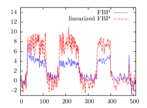
(a)

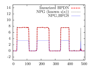
(b)

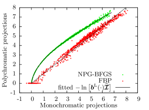
(c)

Figure 5: (a)–(b) The 250th-column profiles of the reconstructions, and (c) the polychromatic measurements as function of the monochromatic projections and corresponding fitted curves.

Note that the nonnegativity constraints on ${\boldsymbol{\alpha}}$ are especially effective in the process of getting good estimation of ${\boldsymbol{\mathcal{I}}}$. Without these constraints, it is even impossible for Step 1) and Step 2) to converge to reasonable place.

V-B X-ray CT Reconstruction from Real Data

We compare the NPG-BFGS and linear FBP methods by applying them to reconstruct two industrial objects containing defects, labeled C-I and C-II, from real fan-beam projections. Here, NPG-BFGS achieves visually good reconstructions for $u=10^{-5}$, presented in Fig. 6.

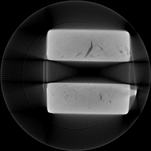
(a) FBP

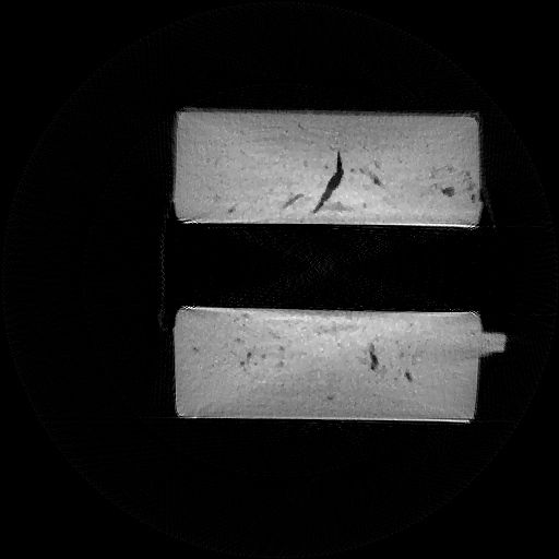
(b) NPG-BFGS

(c) FBP

(d) NPG-BFGS

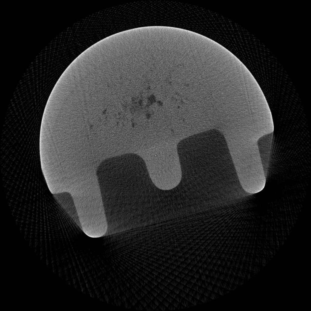
(e) FBP (120 projections)

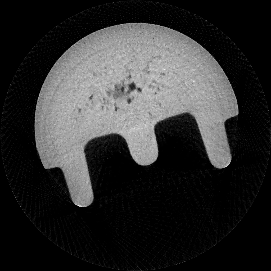
(f) NPG-BFGS (120 projections)

Figure 6: C-I and C-II object reconstructions from fan-beam projections using the FBP and NPG-BFGS methods.

The C-I data set consists of $360$ equi-spaced fan-beam projections with $1\text{\,}\mathrm{\SIUnitSymbolDegree}$ separation collected using an array of $694$ detectors, with distance of X-ray source to the rotation center equal to $3492$ times the detector size. Figs. 6(a) and 6(b) show $512\text{\times}512$ density-map image reconstructions of object C-I using the FBP and NPG-BFGS methods, respectively. The linear FBP reconstruction, which does not account for the polychromatic nature of the X-ray source, suffers from severe streaking (shading that occupies the empty area) and cupping (high intensity along the object’s border) artifacts whereas the NPG-BFGS reconstruction removes these artifacts thanks to accounting for the polychromatic X-ray source.

The C-II data set consists of $360$ equi-spaced fan-beam projections with $1\text{\,}\mathrm{\SIUnitSymbolDegree}$ separation collected using an array of $1380$ detectors, with distance of X-ray source to the rotation center equal to $8696$ times the detector size. Figs. 6(c) and 6(d) show $1024\text{\times}1024$ density-map image reconstructions of object C-II by the FBP and NPG-BFGS methods, respectively. The NPG-BFGS reconstruction removes the streaking and cupping artifacts exhibited by the linear FBP, with enhanced contrast for both the inner defects and object boundary. Figs. 6(e) and 6(f) show the FBP and NPG-BFGS reconstructions from downsampled C-II data set with $120$ equi-spaced fan-beam projections with $3\text{\,}\mathrm{\SIUnitSymbolDegree}$ separation. The FBP reconstruction in Fig. 6(e) exhibits both beam-hardening and aliasing artifacts. In contrast, the NPG-BFGS reconstruction in Fig. 6(f) does not exhibit these artifacts because it accounts for the polychromatic X-ray source and employs signal-sparsity regularization in (29). Indeed, if we reduce the regularization constant $u$ sufficiently, the aliasing effect will occur in the NPG-BFGS reconstruction in Fig. 6(f) as well.

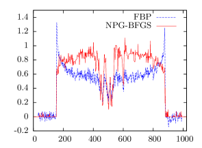
(a) 337th row

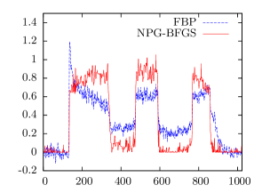
(b) 531st row

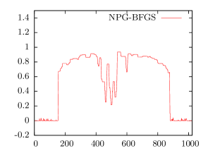
(c) 337th row

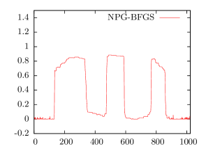
(d) 531st row

Figure 7: C-II object reconstruction profiles with NPG-BFGS reconstructions using the regularization tuning constant (a)–(b) $u=10^{-5}$ and (c)–(d) $u=10^{-4}$.

Fig. 7 shows the reconstruction profiles of the 337th and 531th rows highlighted by the red horizontal lines across Figs. 6(c) and 6(d). Noise in the NPG-BFGS reconstructions can be reduced by increasing the regularization parameter $u$: Figs. 7(c) and 7(d) show the corresponding NPG-BFGS reconstruction profiles for $u=10^{-4}$, which is 10 times that in Figs. 7(a) and 7(b).

Observe that the NPG-BFGS reconstructions of C-I and C-II have higher contrast around the inner region where cracks reside. Indeed, our reconstructions have slightly higher intensity in the center, which is likely due to the detector saturation that lead to measurement truncation; other possible causes could be scattering or noise model mismatch. (We have replicated this slight non-uniformity by applying our reconstruction to simulated truncated measurements.) This effect is visible in C-I reconstruction in Fig. 6(b) and is barely visible in the C-II reconstruction in Fig. 6(d), but can be observed in the profiles in Fig. 7. We leave further verification of causes and potential correction of this problem to future work and note that this issue does not occur in simulated-data examples that we constructed, see Section V-A.

In Fig. 8(a), we show the scatter plots with 1000 randomly selected points representing FBP and NPG-BFGS reconstructions of the C-II object from 360 projections. A few points in the FBP scatter plot with $\ln\mathcal{E}_{n}=0$ and positive monochromatic projections indicate severe streaking artifacts, which we also observed in the simulated example in Section V-A, see Fig. 5(c).

We now illustrate the advantage of using Nesterov’s acceleration in Step 1) of our iteration. Fig. 8(b) shows the objective $f({\boldsymbol{\alpha}},{\boldsymbol{\mathcal{I}}})$ as a function of outer iteration index $i$ for the NPG-BFGS and PG-BFGS methods applied to C-II reconstruction from 360 projections. Thanks to the Nesterov’s acceleration (31b), NPG-BFGS is at least 10 times faster than PG-BFGS, which runs until it reaches the maximum-iteration limit.

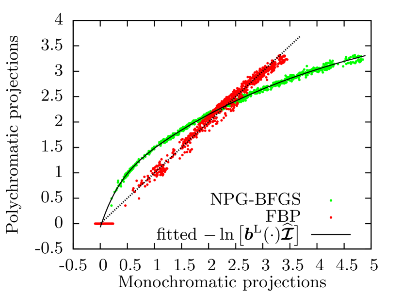
(a)

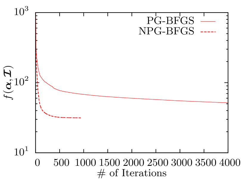
(b)

Figure 8: (a) Polychromatic measurements as functions of monochromatic projections and corresponding fitted inverse linearization curves, and (b) the objective function as a function of the iteration index $i$.

VI Conclusion

We developed a model that requires no more information than the conventional FBP method but is capable of beam-hardening artifact correction. The proposed model, based on the separability of the attenuation, combines the variations of the mass attenuation and X-ray spectrum to mass-attenuation spectrum. This model solves the single material scenario and convert it to a bi-convex optimization problem. We proposed an alternatively descent iterative algorithm to find the solution. We proved the KL properties of the object function under both Gaussian and Poisson noise scenarios, and gave primitive conditions that guarantees the bi-convexity. Numerical experiments on both simulated and real X-ray CT data are presented. Our blind method for sparse X-ray CT reconstruction (i) does not rely on knowledge of the X-ray source spectrum and the inspected material (i.e., its mass-attenuation function), (ii) matches or outperforms non-blind linearization methods that assume perfect knowledge of the X-ray source and material properties. This method is based on our new parsimonious model for polychromatic X-ray CT that exploits separability of attenuation of the inspected object. It is of interest to generalize this model beyond X-ray CT so that it applies to other physical models and measurement scenarios that have separable structure; here, we would construct the most general possible formulation of “separable structure”. For example, our probabilistic model in this paper is closely related to GLMs in statistics [31], and can be viewed as their regularized (nonnegativity- and sparsity-enforcing) generalization as well.

The underlying optimization problem for performing our blind sparse signal reconstruction is biconvex with respect to the density map and mass density spectrum parameters; solving and analyzing bi- and multiconvex problems is of great general interest in optimization theory, see [39] and references therein. An interesting conjecture is that the general version of (ii) holds as a consequence of the separability in the measurement model.

Future work will also include extending our parsimonious mass-attenuation parameterization to multiple materials and developing corresponding reconstruction algorithms.

Appendix A Derivation of the Mass-Attenuation Parameterization

Observe that the mass attenuation $\kappa(\varepsilon)$ and incident energy density $\iota(\varepsilon)$ are both functions of $\varepsilon$, see Fig. 1(a). Thus, to combine the variation of these two functions and reduce the degree of freedom, we rewrite $\iota(\varepsilon)$ as a function of $\kappa$ and set $\kappa$ as the integral variable.

All mass-attenuation functions $\kappa(\varepsilon)$ encountered in practice can be divided into piecewise-continuous segments, where each segment is a differentiable monotonically decreasing function of $\varepsilon$, see [48, Tables 3 and 4] and [50, Sec. 2.3]. The points of discontinuity in $\kappa(\varepsilon)$ are referred to as $K$-edges and are caused by the interaction between photons and $K$ shell electrons, which occurs only when $\varepsilon$ reaches the binding energy of the $K$ shell electron. One example in Fig. 9 is the mass attenuation coefficient curve of iron with a single $K$-edge at $7.11\text{\,}\text{\mathrm{ k }\mathrm{ eV }}$.

If the energy range used in a CT scan does not contain any of the $K$-edges, $\kappa(\varepsilon)$ becomes monotonic and invertible, which we consider first in Appendix A-I. This simple case, depicted in Fig. 1(a), gives the main idea behind our simplified model.

In Appendix A-II, we then consider the general case where the energy range used in a CT scan contains $K$-edges.

A-I Invertible $\kappa(\varepsilon)$

Consider first the simple case where $\kappa(\varepsilon)$ is monotonically decreasing and invertible, as depicted in Fig. 1(a), and define the differentiable inverse of $\kappa(\varepsilon)$ as $\varepsilon(\kappa)$. The change of variables $\varepsilon=\varepsilon(\kappa)$ in the integral expressions (3a) and (3b) yields

$$\mathcal{I}^{\textup{in}} = \int\iota(\varepsilon(\kappa))\lvert\varepsilon^{\prime}(\kappa)\rvert\operatorname{d\!}\kappa$$ (A1a)

$$\mathcal{I}^{\textup{out}} = \int\iota(\varepsilon(\kappa))\lvert\varepsilon^{\prime}(\kappa)\rvert\mathrm{e}^{-\kappa\int\alpha(x,y)\operatorname{d\!}\ell}\operatorname{d\!}\kappa$$ (A1b)

Now, we define

$$\upiota(\kappa)\triangleq\iota(\varepsilon(\kappa))|\varepsilon^{\prime}(\kappa)|$$ (A2)

with $\varepsilon^{\prime}(\kappa)=\operatorname{d\!}\varepsilon(\kappa)/\operatorname{d\!}\kappa$ and obtain (5) by plugging (A2) into (A1).

As shown in Fig. 1(a), the area $\iota(\varepsilon_{j})\Delta\varepsilon_{j}$ depicting the X-ray energy within the $\Delta\varepsilon_{j}$ slot is the same as the corresponding area $\upiota(\kappa_{j})\Delta\kappa_{j}$, the amount of X-ray energy that attenuated at a rate within $\Delta\kappa_{j}$ slot. In the following, we extend the above results to the case where $\kappa(\varepsilon)$ is not monotonic.

A-II Piecewise-continuous $\kappa(\varepsilon)$ with monotonically decreasing invertible segments

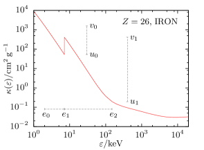
Figure 9: The mass attenuation coefficients $\kappa$ of iron versus the photon energy $\varepsilon$ with a $K$-edge at $7.11\text{\,}\text{\mathrm{ k }\mathrm{ eV }}$.

Define the domain $\mathbb{E}$ of $\varepsilon$ and a sequence of disjoint intervals $\{(e_{m},e_{m+1})\}_{m=0}^{M}$ with $e_{0}=\min(\mathbb{E})$ and $e_{M+1}=\max(\mathbb{E})$, such that in each interval $\kappa(\varepsilon)$ is invertible and differentiable. Here, $\mathbb{E}$ is the support set of the incident X-ray spectrum $\iota(\varepsilon)$ and $(e_{m})_{m=1}^{M}$ are the $M$ $K$-edges in $\mathbb{E}$. Taking Fig. 9 as an example, there is only one $K$-edges at $e_{1}$ given the incident spectrum has its support as $(e_{0},e_{2})$.

The range and inverse of $\kappa(\varepsilon)$ within $(e_{m},e_{m+1})$ are $(u_{m},v_{m})$ and $\varepsilon_{m}(\kappa)$, respectively, with $u_{m}\triangleq\inf_{\varepsilon{\scriptscriptstyle\nearrow}e_{m+1}}\kappa(\varepsilon)<v_{m}\triangleq\sup_{\varepsilon{\scriptscriptstyle\searrow}e_{m}}\kappa(\varepsilon)$. Then, the noiseless measurement in (3b) can be written as

$$\mathcal{I}^{\text{out}} = \sum_{m=0}^{M}\int_{e_{m}}^{e_{m+1}}\iota(\varepsilon)\mathrm{e}^{-\kappa(\varepsilon)\int\alpha(x,y)\operatorname{d\!}\ell}\operatorname{d\!}\varepsilon$$ (A3a)

$$= \sum_{m=0}^{M}\int_{u_{m}}^{v_{m}}\iota(\varepsilon_{m}(\kappa))\left|\varepsilon_{m}^{\prime}(\kappa)\right|\mathrm{e}^{-\kappa\int\alpha(x,y)\operatorname{d\!}\ell}\operatorname{d\!}\kappa$$ (A3b)

$$= \int\sum_{m=0}^{M}1_{(u_{m},v_{m})}(\kappa)\iota(\varepsilon_{m}(\kappa))\left|\varepsilon_{m}^{\prime}(\kappa)\right|\mathrm{e}^{-\kappa\int\alpha(x,y)\operatorname{d\!}\ell}\operatorname{d\!}\kappa.$$ (A3c)

and (5) and (6) follow. Observe that (6) reduces to (A2) when $M=0$.

In this case, suppose there is a $K$-edge with in the range $(\varepsilon_{j_{1}},\varepsilon_{j_{2}})$ and $\kappa(\varepsilon_{j_{1}})=\kappa(\varepsilon_{j_{2}})=\kappa_{j}$, then the amount of X-ray energy, $\upiota(\kappa_{j})\Delta\kappa_{j}$, that attenuated at a rate $\kappa_{j}$ within $\Delta\kappa_{j}$ slot will be the summation of $\iota(\varepsilon_{j_{1}})\Delta\varepsilon_{j_{1}}$ and $\iota(\varepsilon_{j_{2}})\Delta\varepsilon_{j_{2}}$, where slot $\Delta\varepsilon_{j_{1}}$ and $\Delta\varepsilon_{j_{2}}$ correspond to $\Delta\kappa_{j}$.

Appendix B Proofs of Convexity of $\mathcal{L}_{\upiota}({\boldsymbol{\alpha}})$

The proofs of convexity of $\mathcal{L}_{\upiota}({\boldsymbol{\alpha}})$ for both the lognormal and Poisson noise measurement models share a common component, which we first introduce as a lemma.

Lemma 7

For $\upiota(\kappa)$ that satisfy Assumption 1, the following holds:

w $$\triangleq {\iint}\biggl{[}\mu\kappa-\frac{q^{j_{0}}}{(q^{j_{0}}+1)^{2}}\left({\mu+\kappa}\right)^{2}\biggr{]}\upiota(\kappa)\upiota(\mu)h(\kappa+\mu)\operatorname{d\!}\mu\operatorname{d\!}\kappa$$ (B1a)

$$\geq 0$$ (B1b)

for $q>1$ [as in (10b)] and any nonnegative function $h\mathrel{\mathop{\mathchar 58\relax}}\mathbb{R}\rightarrow\mathbb{R}_{+}$.

Proof:

In Fig. 10, the $(\mu,\kappa)$ coordinates of $P$, $B$ and $N$ are $(\kappa_{0},0)$, $(\kappa_{j_{0}},0)$ and $(\kappa_{J+1},0)$, respectively; the line $OS$ is defined by $\kappa=\mu$.

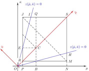
Figure 10: Integral region illustration.

Considering the finite support set of $\iota(\kappa)$, the effective integral range is $[\kappa_{0},\kappa_{J+1}]^{2}$, which is the rectangle $RMSJ$ in Fig. 10. Using the symmetry between $\kappa$ and $\mu$ in (B1a), we change the integral variables of (B1a) by rotating the coordinates by $90^{\circ}$ using

$$\mu = \frac{1}{\sqrt{2}}(\bar{\mu}-\bar{\kappa})$$ (B2a)

$$\kappa = \frac{1}{\sqrt{2}}(\bar{\mu}+\bar{\kappa})$$ (B2b)

which yields

w $$= \frac{1}{2}\int\displaylimits_{\sqrt{2}\kappa_{0}}^{\sqrt{2}\kappa_{J+1}}\int\displaylimits_{-g(\bar{\mu})}^{g(\bar{\mu})}\bar{w}(\bar{\mu},\bar{\kappa})\operatorname{d\!}\bar{\kappa}\>h\bigl{(}\sqrt{2}\bar{\mu}\bigr{)}\operatorname{d\!}\bar{\mu}$$ (B3a)

$$= \int\displaylimits_{\sqrt{2}\kappa_{0}}^{\sqrt{2}\kappa_{J+1}}\int\displaylimits_{0}^{g(\bar{\mu})}\bar{w}(\bar{\mu},\bar{\kappa})\operatorname{d\!}\bar{\kappa}\>h\bigl{(}\sqrt{2}\bar{\mu}\bigr{)}\operatorname{d\!}\bar{\mu}$$ (B3b)

where

$$\bar{w}(\bar{\mu},\bar{\kappa}) \triangleq z(\bar{\mu},\bar{\kappa})\upiota\left({\frac{\bar{\mu}+\bar{\kappa}}{\sqrt{2}}}\right)\upiota\left({\frac{\bar{\mu}-\bar{\kappa}}{\sqrt{2}}}\right)$$ (B3c)

$$z(\bar{\mu},\bar{\kappa}) \triangleq \left({\frac{q^{j_{0}}-1}{q^{j_{0}}+1}}\right)^{2}\bar{\mu}^{2}-\bar{\kappa}^{2}$$ (B3d)

$$g(\bar{\mu}) \triangleq \begin{cases}\bar{\mu}-\sqrt{2}\kappa_{0},&\bar{\mu}\leq\frac{1}{\sqrt{2}}(\kappa_{0}+\kappa_{J+1})\\ \sqrt{2}\kappa_{J+1}-\bar{\mu},&\bar{\mu}>\frac{1}{\sqrt{2}}(\kappa_{0}+\kappa_{J+1})\end{cases}$$ (B3e)

and (B3b) follows because (B3c) is even symmetric with respect to $\bar{\kappa}$. Now, the integration region is reduced to the triangle $RSJ$ in Fig. 10.

Note that $z(\bar{\mu},\bar{\kappa})\geq 0$ in the cone between lines $OH$ and $OI$, [both of which are specified by $z(\bar{\mu},\bar{\kappa})=0$], which implies that $\bar{w}\left({\bar{\mu},\bar{\kappa}}\right)\geq 0$ within $RCE$ and $CSQ$; hence, the integrals of $\bar{w}(\bar{\mu},\bar{\kappa})h\bigl{(}\sqrt{2}\bar{\mu}\bigr{)}$ over $RCE$ and $CSQ$ are nonnegative and, consequently,

$$\textup{w}\geq\iint\limits_{\mathcal{R}}\bar{w}(\bar{\mu},\bar{\kappa})\operatorname{d\!}\bar{\kappa}\;h\bigl{(}\sqrt{2}\bar{\mu}\bigr{)}\operatorname{d\!}\bar{\mu}.$$ (B4)

where

$$\mathcal{R}\triangleq\left\{(\bar{\mu},\bar{\kappa})\left|{\,\frac{\bar{\mu}-\bar{\kappa}}{\sqrt{2}}\in[\kappa_{0},\kappa_{j_{0}}],\;\frac{\bar{\mu}+\bar{\kappa}}{\sqrt{2}}\in[\kappa_{j_{0}},\kappa_{J+1}]}\right.\right\}$$ (B5)

is our new integration region, which is the rectangle $ECQJ$ in Fig. 10.

Define

$$c\triangleq\frac{\sqrt{2}}{1+q^{j_{0}}}.$$ (B6)

Now, we split the inner integral over $\bar{\kappa}$ on the right-hand side of (B4) for fixed $\bar{\mu}$ into two regions: $z(\bar{\mu},\bar{\kappa})\geq 0$ and $z(\bar{\mu},\bar{\kappa})<0$, i.e., trapezoid $ECQI$ and triangle $EIJ$, and prove that the positive contribution of the integral over $ECQI$ is larger than the negative contribution of the integral over the $EIJ$.

Note that the line $OI$ is specified by $z(\bar{\mu},\bar{\kappa})=0$ and the $(\mu,\kappa)$-coordinate of $I$ in Fig. 10 is thus $(\kappa_{J+1-j_{0}},\kappa_{J+1})$. Hence, under Assumption 1, region $ECQI\subseteq(\mathcal{K}_{\text{low}}\cup\mathcal{K}_{\text{mid}})\times\mathcal{K}_{\text{high}}$ and region $EIJ\subseteq\mathcal{K}_{\text{low}}\times\mathcal{K}_{\text{high}}$. Therefore, the following hold within $\mathcal{R}$:

• When $z(\bar{\mu},\bar{\kappa})\geq 0$, i.e., in region $ECQI$,

  $$\left.{\upiota(\kappa)\,}\right|_{\kappa=\frac{\bar{\mu}+\bar{\kappa}}{\sqrt{2}}} \geq \upiota\bigl{(}cq^{j_{0}}\bar{\mu}\bigr{)}$$ (B7a)

  $$\left.{\upiota(\mu)\,}\right|_{\mu=\frac{\bar{\mu}-\bar{\kappa}}{\sqrt{2}}} \geq \upiota\bigl{(}c\bar{\mu}\bigr{)}$$ (B7b)

  where (B7a) follows because $$\kappa=\frac{\bar{\mu}+\bar{\kappa}}{\sqrt{2}} \kappa_{j_{0}} cq^{j_{0}}\bar{\mu}\in[\kappa_{j_{0}},\kappa_{J+1}] \kappa\in\mathcal{K}_{\text{high}} \upiota(\kappa) \mathcal{K}_{\text{high}} \mu=\frac{\bar{\mu}-\bar{\kappa}}{\sqrt{2}} c\bar{\mu}\in[\kappa_{0},\kappa_{J+1-j_{0}}] \kappa_{j_{0}} \mu \mathcal{K}_{\text{low}} \upiota(\kappa) \mathcal{K}_{\text{mid}} \upiota(\kappa) (c\bar{\mu},cq^{j_{0}}\bar{\mu}) (\mu,\kappa) OI \bar{\mu} (\bar{\mu},\bar{\kappa})$$ takes values between and , i.e., and decreases in ; (B7b) follows because takes values between and , i.e., crosses ( increasing) and ( keeping high) regions, see (15b). Here, is the -coordinate of one point on line specified by in -coordinate system.

• When $z(\bar{\mu},\bar{\kappa})<0$, i.e., in region $EIJ$,

  $$\left.{\upiota(\kappa)\,}\right|_{\kappa=\frac{\bar{\mu}+\bar{\kappa}}{\sqrt{2}}} < \upiota\bigl{(}cq^{j_{0}}\bar{\mu}\bigr{)}$$ (B7c)

  $$\left.{\upiota(\mu)\,}\right|_{\mu=\frac{\bar{\mu}-\bar{\kappa}}{\sqrt{2}}} < \upiota\bigl{(}c\bar{\mu}\bigr{)}$$ (B7d)

  where (B7c) follows because $\kappa=\frac{\bar{\mu}+\bar{\kappa}}{\sqrt{2}}>cq^{j_{0}}\bar{\mu}$, i.e., $\kappa\in\mathcal{K}_{\text{high}}$ and (B7d) follows because $\mu=\frac{\bar{\mu}-\bar{\kappa}}{\sqrt{2}}<c\bar{\mu}$, i.e., $\mu\in\mathcal{K}_{\text{low}}$.

By combining (B7) with (B4), we have

w $$\geq \iint_{\mathcal{R}}{z(\bar{\mu},\bar{\kappa})\operatorname{d\!}\bar{\kappa}\;\bar{h}(\bar{\mu})}\operatorname{d\!}\bar{\mu}$$ (B8a)

$$= \int\limits_{\frac{\kappa_{0}+\kappa_{j_{0}}}{\sqrt{2}}}^{\frac{\kappa_{J+1}+\kappa_{J+1-j_{0}}}{\sqrt{2}}}\int\displaylimits_{\{\bar{\kappa}\,\mid\,(\bar{\mu},\bar{\kappa})\in\mathcal{R}\}}z(\bar{\mu},\bar{\kappa})\operatorname{d\!}\bar{\kappa}\operatorname{d\!}\bar{\mu}$$ (B8b)

with

$$\bar{h}(\bar{\mu}) \triangleq \upiota\bigl{(}cq^{j_{0}}\bar{\mu}\bigr{)}\upiota\bigl{(}c\bar{\mu}\bigr{)}h\bigl{(}\sqrt{2}\bar{\mu}\bigr{)}$$ (B8c)

$$\geq 0.$$

It easy to verify that $\int\displaylimits_{\{\bar{\kappa}\,\mid\,(\bar{\mu},\bar{\kappa})\in\mathcal{R}\}}z(\bar{\mu},\bar{\kappa})\operatorname{d\!}\bar{\kappa}$ is an increasing function of $\bar{\mu}$ over the range of the outer integral $\left[\frac{\kappa_{0}+\kappa_{j_{0}}}{\sqrt{2}},\frac{\kappa_{J+1}+\kappa_{J+1-j_{0}}}{\sqrt{2}}\right]$ and, consequently,

$$\int\displaylimits_{\{\bar{\kappa}\,\mid\,(\bar{\mu},\bar{\kappa})\in\mathcal{R}\}}z(\bar{\mu},\bar{\kappa})\operatorname{d\!}\bar{\kappa}\geq 0$$ (B9)

where the equality is attained for $\bar{\mu}=(\kappa_{0}+\kappa_{j_{0}})/\sqrt{2}$. Finally, (B1) follows from (B8a) and (B9). ∎

This proof of convexity of Lemma 7 is conservative as we loose the positve integral in region $RCE$ and $CSQ$ to zero.

Now, we use Lemma 7 to prove the convexity of $\mathcal{L}_{\upiota}({\boldsymbol{\alpha}})$ in Lemmas 2 and 4. Note that the mass-attenuation spectrum $\upiota(\kappa)$ is considered known in Lemmas 2 and 4 and define $\xi(\cdot)\triangleq\upiota^{\textup{L}}(\cdot)$ and the corresponding first and second derivatives:

$$\dot{\xi}(s) = \left({-\kappa\upiota}\right)^{\textup{L}}(s),$$ ¨ξ(s) = (κ^2ι)^L(s). (B10)

Observe that ${\boldsymbol{\mathcal{I}}}^{\textup{out}}=\left({\mathcal{I}^{\textup{out}}_{n}}\right)_{n=1}^{N}=\xi_{\circ}(\Phi{\boldsymbol{\alpha}})=\bigl{(}\xi(\boldsymbol{\phi}^{T}_{n}{\boldsymbol{\alpha}})\bigr{)}_{n=1}^{N}$. For notational simplicity, we omit the dependence of ${\boldsymbol{\mathcal{I}}}^{\textup{out}}$ on ${\boldsymbol{\alpha}}$ and ${\boldsymbol{\mathcal{I}}}$ and use ${\boldsymbol{\mathcal{I}}}^{\textup{out}}$ and $\xi_{\circ}(\Phi{\boldsymbol{\alpha}})$ interchangeably.

Proof:

We use the identities

$$\frac{\partial\xi_{\circ}(\Phi{\boldsymbol{\alpha}})}{\partial{\boldsymbol{\alpha}}^{T}} = \operatorname{diag}\bigl{(}\dot{\xi}_{\circ}(\Phi{\boldsymbol{\alpha}})\bigr{)}\Phi$$ (B11a)

$$\frac{\partial\xi(\boldsymbol{\phi}^{T}_{n}{\boldsymbol{\alpha}})}{\partial{\boldsymbol{\alpha}}\partial{\boldsymbol{\alpha}}^{T}} = \ddot{\xi}(\boldsymbol{\phi}^{T}_{n}{\boldsymbol{\alpha}})\boldsymbol{\phi}_{n}\boldsymbol{\phi}_{n}^{T}$$ (B11b)

to compute the gradient and Hessian of the lognormal NLL in (14b):

$$\frac{\partial\mathcal{L}_{\upiota}({\boldsymbol{\alpha}})}{\partial{\boldsymbol{\alpha}}} = \Phi^{T}\operatorname{diag}\bigl{(}\dot{\xi}_{\circ}(\Phi{\boldsymbol{\alpha}})\bigr{)}\operatorname{diag}^{-1}\left({{\boldsymbol{\mathcal{I}}}^{\textup{out}}}\right)\left({\ln_{\circ}{\boldsymbol{\mathcal{I}}}^{\textup{out}}-\ln_{\circ}{\boldsymbol{\mathcal{E}}}}\right)$$ (B12a)

$$\frac{\partial\mathcal{L}_{\upiota}({\boldsymbol{\alpha}})}{\partial{\boldsymbol{\alpha}}\partial{\boldsymbol{\alpha}}^{T}} = \Phi^{T}\operatorname{diag}^{-2}\left({{\boldsymbol{\mathcal{I}}}^{\textup{out}}}\right)\operatorname{diag}\left({\boldsymbol{w}}\right)\Phi$$ (B12b)

where the $$N\times 1 \boldsymbol{w}=\left({w_{n}}\right)_{n=1}^{N}$$ vector is defined as

$$w_{n} = \left.{\dot{\xi}^{2}(s)+t(s)\left({\ln\mathcal{I}_{n}^{\textup{out}}-\ln\mathcal{E}_{n}}\right)\,}\right|_{s=\boldsymbol{\phi}_{n}^{T}{\boldsymbol{\alpha}}}$$ (B12c)

$$t(s) \triangleq \xi(s)\ddot{\xi}(s)-\dot{\xi}^{2}(s).$$ (B12d)

For $s>0$,

$$t(s) = \int\upiota(\kappa)\mathrm{e}^{-s\kappa}\operatorname{d\!}\kappa\int\kappa^{2}\upiota(\kappa)\mathrm{e}^{-s\kappa}\operatorname{d\!}\kappa-\biggl{[}\int\kappa\upiota(\kappa)\mathrm{e}^{-s\kappa}\operatorname{d\!}\kappa\biggr{]}^{2}\geq 0$$ (B13a)

where we used the Laplace-transform identity for derivatives (1c) and the inequality follows by using the Cauchy-Schwartz inequality. We can write $$t(s)$$ as

$$t(s)=\frac{1}{2}\iint(\kappa-\mu)^{2}\upiota(\kappa)\upiota(\mu)\mathrm{e}^{-s(\kappa+\mu)}\operatorname{d\!}\kappa\operatorname{d\!}\mu$$ (B13b)

which also implies that $t(s)\geq 0$. We obtain (B13b) by using the Laplace-transform identity for derivatives (1c), combining the multiplication of the integrals, and symmetrizing the integral expressions by replacing $\kappa^{2}$ with $(\kappa^{2}+\mu^{2})/2$.

According to (18a), $\ln\mathcal{I}^{\textup{out}}_{n}-\ln\mathcal{E}_{n}\geq-U$, see also (18b). Because of positivity of $t(s)$ for $s\geq 0$,

$$w_{n} \geq \left.{\dot{\xi}^{2}(s)-Ut(s)\,}\right|_{s=\boldsymbol{\phi}_{n}^{T}{\boldsymbol{\alpha}}}$$ (B14a)

$$= {\iint}\biggl{[}\mu\kappa-U\frac{(\mu-\kappa)^{2}}{2}\biggr{]}\upiota(\mu)\upiota(\kappa)\mathrm{e}^{-(\mu+\kappa)\boldsymbol{\phi}_{n}^{T}{\boldsymbol{\alpha}}}\operatorname{d\!}\kappa\operatorname{d\!}\mu$$ (B14b)

$$= \left({\frac{q^{j_{0}}+1}{q^{j_{0}}-1}}\right)^{2}{\iint}\biggl{[}\mu\kappa-\frac{q^{j_{0}}}{(q^{j_{0}}+1)^{2}}(\mu+\kappa)^{2}\biggr{]}\upiota(\mu)\upiota(\kappa)\mathrm{e}^{-(\mu+\kappa)\boldsymbol{\phi}_{n}^{T}{\boldsymbol{\alpha}}}\operatorname{d\!}\kappa\operatorname{d\!}\mu$$ (B14c)

where (B14b) is obtained by plugging (B13b) into (B14a), and we have used the definition of $U$ (18b) in (B14c).

Using Lemma 7 with $h(\kappa)=\mathrm{e}^{-\kappa\boldsymbol{\phi}_{n}^{T}{\boldsymbol{\alpha}}}$, we have $w_{n}\geq 0$ for all $n$. Therefore, the Hessian matrix (B12b) of $\mathcal{L}_{\upiota}({\boldsymbol{\alpha}})$ is positive semidefinite. ∎

Proof:

We use the identities (B11) to compute the gradient and Hessian of the Poisson NLL (23):

$$\frac{\partial\mathcal{L}_{\upiota}({\boldsymbol{\alpha}})}{\partial{\boldsymbol{\alpha}}} = \Phi^{T}\operatorname{diag}\bigl{(}\dot{\xi}_{\circ}\bigl{(}\Phi{\boldsymbol{\alpha}}\bigr{)}\bigr{)}\bigl{[}\boldsymbol{1}-\operatorname{diag}^{-1}\left({{\boldsymbol{\mathcal{I}}}^{\textup{out}}}\right){\boldsymbol{\mathcal{E}}}\bigr{]}$$ (B15a)

$$\frac{\partial\mathcal{L}_{\upiota}({\boldsymbol{\alpha}})}{\partial{\boldsymbol{\alpha}}\partial{\boldsymbol{\alpha}}^{T}} = \Phi^{T}\operatorname{diag}^{-2}\left({{\boldsymbol{\mathcal{I}}}^{\textup{out}}}\right)\operatorname{diag}\left({{\boldsymbol{\mathcal{E}}}}\right)\operatorname{diag}\left({\boldsymbol{x}}\right)\Phi$$ (B15b)

where the $$N\times 1 \boldsymbol{x}=\left({x_{n}}\right)_{n=1}^{N}$$ vector is defined as

$$x_{n} = \left.{\dot{\xi}^{2}\bigl{(}s\bigr{)}+\ddot{\xi}\bigl{(}s\bigr{)}\xi(s)\left({\frac{\mathcal{I}^{\textup{out}}_{n}}{\mathcal{E}_{n}}-1}\right)\,}\right|_{s=\boldsymbol{\phi}_{n}^{T}{\boldsymbol{\alpha}}}.$$ (B15c)

Since $\mathcal{I}_{n}^{\textup{out}}\geq(1-V)\mathcal{E}_{n}\geq 0$ according to (24a), we have

$$\frac{\mathcal{I}^{\textup{out}}_{n}}{\mathcal{E}_{n}}-1\geq-V.$$ (B16)

Now,

$$x_{n} \geq \iint\left({\mu\kappa-\kappa^{2}V}\right)\upiota(\mu)\upiota(\kappa)\mathrm{e}^{-(\mu+\kappa)\boldsymbol{\phi}_{n}^{T}{\boldsymbol{\alpha}}}\operatorname{d\!}\kappa\operatorname{d\!}\mu$$ (B17a)

$$= {\iint}\Bigl{(}{\mu\kappa-\frac{\mu^{2}+\kappa^{2}}{2}V}\Bigr{)}\upiota(\mu)\upiota(\kappa)\mathrm{e}^{-(\mu+\kappa)\boldsymbol{\phi}_{n}^{T}{\boldsymbol{\alpha}}}\operatorname{d\!}\kappa\operatorname{d\!}\mu$$ (B17b)

$$\geq \frac{(q^{j_{0}}+1)^{2}}{q^{2j_{0}}+1}{\iint}\Bigl{[}\mu\kappa-\frac{q^{j_{0}}}{(q^{j_{0}}+1)^{2}}(\mu+\kappa)^{2}\Bigr{]}\upiota(\mu)\upiota(\kappa)\mathrm{e}^{-(\mu+\kappa)\boldsymbol{\phi}_{n}^{T}{\boldsymbol{\alpha}}}\operatorname{d\!}\kappa\operatorname{d\!}\mu$$ (B17c)

$$\geq 0$$ (B17d)

where (B17a) follows by applying inequality (B16) to (B15c), using the Laplace-transform identity for derivatives (1c), and combining the multiplication of the integrals, and (B17b) is due to the symmetry with respect to $\mu$ and $\kappa$ by replacing $\kappa^{2}$ with $(\kappa^{2}+\mu^{2})/2$. Now, plug (24b) into (B17b) and apply Lemma 7 with $h(\kappa)=\mathrm{e}^{-\kappa\boldsymbol{\phi}_{n}^{T}{\boldsymbol{\alpha}}}$ to conclude (B17d). Therefore, the Hessian of $\mathcal{L}_{\upiota}({\boldsymbol{\alpha}})$ in (B15b) is positive semidefinite. ∎

Appendix C Proofs of KL Property and Convergence of PG-BFGS Iteration

Proof:

According to [39], real-analytic function [51], semialgebraic functions [52] and their summations satisfy the KL property automatically. Therefore, the proof consists two parts:

1. The NLLs in (13) and (22), are both real-analytic functions of $({\boldsymbol{\alpha}},{\boldsymbol{\mathcal{I}}})$ on $\mathbb{C}\subseteq\operatorname{dom}(f)$;

2. Both $r({\boldsymbol{\alpha}})$ in (29b)–(29a) and $\mathbb{I}_{[0,+\infty)}({\boldsymbol{\mathcal{I}}})$ are semialgebraic functions;

and, consequently, the objective function $f({\boldsymbol{\alpha}},{\boldsymbol{\mathcal{I}}})$ satisfies the KL property.

Real-analytic NLLs. The NLLs in (13) and (22) are in the form of weighted summations of terms ${\boldsymbol{b}}^{\textup{L}}(\boldsymbol{\phi}_{n}^{T}{\boldsymbol{\alpha}}){\boldsymbol{\mathcal{I}}}$, $\ln\bigl{[}{\boldsymbol{b}}^{\textup{L}}(\boldsymbol{\phi}_{n}^{T}{\boldsymbol{\alpha}}){\boldsymbol{\mathcal{I}}}\bigr{]}$, and $\ln^{2}\bigl{[}{\boldsymbol{b}}^{\textup{L}}(\boldsymbol{\phi}_{n}^{T}{\boldsymbol{\alpha}}){\boldsymbol{\mathcal{I}}}\bigr{]}$ for $n=1,2,\ldots,N$. Weighted summation of real-analytic functions is real-analytic; hence, we need to prove that the following are real-analytic functions:

$$l_{1}(t) = {\boldsymbol{b}}^{\textup{L}}\bigl{(}\boldsymbol{\phi}^{T}({\boldsymbol{\alpha}}+t{\boldsymbol{\gamma}})\bigr{)}({\boldsymbol{\mathcal{I}}}+t{\boldsymbol{\mathcal{J}}})$$ (C1a)

$$l_{2}(t) = \ln\bigl{[}{\boldsymbol{b}}^{\textup{L}}\bigl{(}\boldsymbol{\phi}^{T}({\boldsymbol{\alpha}}+t{\boldsymbol{\gamma}})\bigr{)}({\boldsymbol{\mathcal{I}}}+t{\boldsymbol{\mathcal{J}}})\bigr{]}=\ln l_{1}(t)$$ (C1b)

$$l_{3}(t) = l_{2}^{2}(t)$$ (C1c)

Since $\left({l_{i}(t)}\right)_{i=1}^{3}$ are smooth, it is sufficient to prove that the $m$th derivatives, $l_{i}^{(m)}(t)$, are bounded for all $m$, $({\boldsymbol{\alpha}},{\boldsymbol{\mathcal{I}}})$, $({\boldsymbol{\gamma}},{\boldsymbol{\mathcal{J}}})$ and $t$ such that $({\boldsymbol{\alpha}}+t{\boldsymbol{\gamma}},{\boldsymbol{\mathcal{I}}}+t{\boldsymbol{\mathcal{J}}})\in\operatorname{dom}(f)$. The $m$th derivative of $l_{1}(t)$ is

$$l_{1}^{(m)}=(\boldsymbol{\phi}^{T}{\boldsymbol{\gamma}})^{m}\left({(-\kappa)^{m}{\boldsymbol{b}}}\right)^{\textup{L}}({\boldsymbol{\alpha}}+t{\boldsymbol{\gamma}})({\boldsymbol{\mathcal{I}}}+t{\boldsymbol{\mathcal{J}}})+m(\boldsymbol{\phi}^{T}{\boldsymbol{\gamma}})^{m-1}\left({(-\kappa)^{m-1}{\boldsymbol{b}}}\right)^{\textup{L}}({\boldsymbol{\alpha}}+t{\boldsymbol{\gamma}}){\boldsymbol{\mathcal{J}}}$$ (C2)

which is bounded for any ${\boldsymbol{\alpha}}$, ${\boldsymbol{\mathcal{I}}}$, ${\boldsymbol{\gamma}}$, ${\boldsymbol{\mathcal{J}}}$ and $t$ such that $({\boldsymbol{\alpha}}+t{\boldsymbol{\gamma}},{\boldsymbol{\mathcal{I}}}+t{\boldsymbol{\mathcal{J}}})$ is in one of compact subsets $\mathbb{C}\subseteq\operatorname{dom}(f)$. For any compact set $\mathbb{C}\subseteq\operatorname{dom}(f)$, there exists $\epsilon>0$ such that $l_{1}(t)\geq\epsilon$, for all $({\boldsymbol{\alpha}}+t{\boldsymbol{\gamma}},{\boldsymbol{\mathcal{I}}}+t{\boldsymbol{\mathcal{J}}})\in\mathbb{C}$. Hence, $\ln(\cdot)$ and $(\cdot)^{2}$ are analytic on $[\epsilon,+\infty)$. Now, since the compositions and products of analytic functions are analytic [53, Ch. 1.4], we have that both $l_{2}(t)$ and $l_{3}(t)$ are analytic.

Therefore, the NLLs in both (13) and (22) are analytic.

Semialgebraic regularization terms. According to [39], i) the $\ell_{2}$ and $\ell_{1}$ norms $\lVert\cdot\rVert_{2}$ and $\lVert\cdot\rVert_{1}$ are semialgebraic, ii) indicator function $\mathbb{I}_{[0,+\infty)}(\cdot)$ is semialgebraic, iii) finite sums and products of semialgebraic functions are semialgebraic, and iv) the composition of semialgebraic functions are semialgebraic. Therefore, $\lVert\Psi^{T}{\boldsymbol{\alpha}}\rVert_{1}$, $\mathbb{I}_{[0,+\infty)}({\boldsymbol{\alpha}})$ and $\mathbb{I}_{[0,+\infty)}({\boldsymbol{\mathcal{I}}})$ are all semialgebraic. Since $\sqrt{\sum_{j\in\mathcal{N}_{i}}(\alpha_{i}-\alpha_{j})^{2}}=\left\lVert P_{i}{\boldsymbol{\alpha}}\right\rVert_{2}$ for some matrix $P_{i}$ is semialgebraic, $r({\boldsymbol{\alpha}})$ in (29a) is semialgebraic.

Finally, according to [39], sum of real-analytic and semialgebraic functions satisfies KL property. Therefore, $f({\boldsymbol{\alpha}},{\boldsymbol{\mathcal{I}}})$ satisfies the KL property on $\operatorname{dom}(f)$. ∎

Proof:

We apply [39, Lemma 2.6] to establish the convergence of $\bigl{\{}\bigl{(}{\boldsymbol{\alpha}}^{(i)},{\boldsymbol{\mathcal{I}}}^{(i)}\bigr{)}\bigr{\}}_{i=1}^{+\infty}$.

Since (13), $r({\boldsymbol{\alpha}})$ in (29) and $\mathbb{I}_{[0,+\infty)}({\boldsymbol{\mathcal{I}}})$ are lower-bounded, we only need to prove that $\eqref{eq:poissNLL}$ is lower-bounded. By using the fact that $\ln x\leq x-1$, we have

$$\mathcal{L}({\boldsymbol{\alpha}},{\boldsymbol{\mathcal{I}}}) = \boldsymbol{1}^{T}\left[{\boldsymbol{\mathcal{I}}}^{\textup{out}}({\boldsymbol{\alpha}},{\boldsymbol{\mathcal{I}}})-{\boldsymbol{\mathcal{E}}}\right]-\sum_{n=1}^{N}\mathcal{E}_{n}\ln\frac{\mathcal{I}_{n}^{\textup{out}}({\boldsymbol{\alpha}},{\boldsymbol{\mathcal{I}}})}{\mathcal{E}_{n}}$$ (C3a)

$$\geq 0$$ (C3b)

According to the assumption, we have $f({\boldsymbol{\alpha}},{\boldsymbol{\mathcal{I}}})$ strongly convex over ${\boldsymbol{\mathcal{I}}}$ and bounded the step size $\beta^{(i)}$. So, there exist constants $0<l<L<+\infty$ such that

$$f\bigl{(}{\boldsymbol{\alpha}}^{(i+1)},{\boldsymbol{\mathcal{I}}}^{(i)}\bigr{)}-f\bigl{(}{\boldsymbol{\alpha}}^{(i+1)},{\boldsymbol{\mathcal{I}}}^{(i+1)}\bigr{)} \geq \frac{l}{2}\bigl{\|}{\boldsymbol{\mathcal{I}}}^{(i)}-{\boldsymbol{\mathcal{I}}}^{(i+1)}\bigr{\|}_{2}^{2}$$ (C4a)

$$L \geq \frac{1}{\beta^{(i)}}\geq l.$$ (C4b)

Hence, we have verified all conditions of [39, Lemma 2.6]. ∎

References

- [1] Wim Dewulf, Ye Tan and Kim Kiekens “Sense and non-sense of beam hardening correction in CT metrology” In CIRP Annals 61.1, 2012, pp. 495–498 DOI: http://dx.doi.org/10.1016/j.cirp.2012.03.013
- [2] Ge Wang, Hengyong Yu and Bruno De Man “An outlook on x-ray CT research and development” In Med. Phys. 35.3, 2008, pp. 1051–1064
- [3] Z. Ying, R. Naidu and C. R. Crawford “Dual energy computed tomography for explosive detection” In J. X-Ray Sci. Technol. 14.4, 2006, pp. 235–256
- [4] J.F. Barrett and N. Keat “Artifacts in CT Recognition and avoidance” In Radiographics 24.6 Radiological Society of North America, 2004, pp. 1679–1691
- [5] J. Hsieh “Computed Tomography: Principles, Design, Artifacts, and Recent Advances” Bellingham, WA: SPIE, 2009
- [6] Renliang Gu and Aleksandar Dogandžić “Beam Hardening Correction Via Mass Attenuation Discretization” In Proc. IEEE Int. Conf. Acoust., Speech, Signal Process., 2013, pp. 1085–1089
- [7] Renliang Gu and Aleksandar Dogandžić “Polychromatic Sparse Image Reconstruction and Mass Attenuation Spectrum Estimation via B-Spline Basis Function Expansion” In Rev. Prog. Quant. Nondestr. Eval. 34 1650, AIP Conf. Proc., 2015, pp. 1707–1716
- [8] Francis A Jenkins and Harvey E White “Fundamentals of Optics” New York: McGraw-Hill, 1957
- [9] Johan Nuyts, Bruno De Man, Jeffrey A Fessler, Wojciech Zbijewski and Freek J Beekman “Modelling the physics in the iterative reconstruction for transmission computed tomography” In Phys. Med. Biol. 58.12, 2013, pp. R63–R96
- [10] A. C. Kak and M. Slaney “Principles of Computerized Tomographic Imaging” New York: IEEE Press, 1988
- [11] M. Krumm, S. Kasperl and M. Franz “Reducing non-linear artifacts of multi-material objects in industrial 3D computed tomography” In NDT & E Int. 41.4, 2008, pp. 242–251 DOI: 10.1016/j.ndteint.2007.12.001
- [12] Idris A Elbakri and Jeffrey A Fessler “Statistical image reconstruction for polyenergetic X-ray computed tomography” In IEEE Trans. Med. Imag. 21.2, 2002, pp. 89–99 DOI: 10.1109/42.993128
- [13] Idris A Elbakri and Jeffrey A Fessler “Segmentation-free statistical image reconstruction for polyenergetic X-ray computed tomography with experimental validation” In Phys. Med. Biol. 48.15, 2003, pp. 2453–2477
- [14] G. Van Gompel, K. Van Slambrouck, M. Defrise, K.J. Batenburg, J. Mey, J. Sijbers and J. Nuyts “Iterative correction of beam hardening artifacts in CT” In Med. Phys. 38, 2011, pp. S36–S49 DOI: 10.1118/1.3577758
- [15] Renliang Gu and Aleksandar Dogandžić “Sparse X-ray CT Image Reconstruction and Blind Beam Hardening Correction via Mass Attenuation Discretization” In Proc. IEEE Int. Workshop Comput. Advances Multi-Sensor Adaptive Process., 2013, pp. 244–247
- [16] G. T. Herman “Correction for beam hardening in computed tomography” In Phys. Med. Biol. 24.1 IOP Publishing, 1979, pp. 81–106
- [17] Kuidong Huang, Dinghua Zhang and Mingjun Li “Noise Suppression Methods in Beam Hardening Correction for X-Ray Computed Tomography” In Proc. 2nd Int. Congress Image Signal Process., 2009, pp. 1–5 DOI: 10.1109/CISP.2009.5303506
- [18] Andrew M. Kingston, Glenn R. Myers and Trond K. Varslot “X-ray beam hardening correction by minimising reprojection distance” In Developments in X-ray Tomography VIII 8506, Proc. SPIE, 2012
- [19] O. Nalcioglu and R. Y. Lou “Post-reconstruction method for beam hardening in computerised tomography” In Med. Phys. Biol. 24.2, 1979, pp. 330–340
- [20] B. De Man, J. Nuyts, P. Dupont, G. Marchal and P. Suetens “An iterative maximum-likelihood polychromatic algorithm for CT” In IEEE Trans. Med. Imag. 20.10 IEEE, 2001, pp. 999–1008
- [21] Idris A Elbakri and Jeffrey A Fessler “Efficient and accurate likelihood for iterative image reconstruction in X-ray computed tomography” In Proc. SPIE Med. Imag. 5032, 2003, pp. 1839–1850
- [22] Bruce R Whiting, Parinaz Massoumzadeh, Orville A Earl, Joseph A O’Sullivan, Donald L Snyder and Jeffrey F Williamson “Properties of preprocessed sinogram data in X-ray computed tomography” In Med. Phys. 33.9 American Association of Physicists in Medicine, 2006, pp. 3290–3303
- [23] Jingyan Xu and Benjamin MW Tsui “Quantifying the importance of the statistical assumption in statistical X-ray CT image reconstruction” In IEEE Trans. Med. Imag. 33.1 IEEE, 2014, pp. 61–73
- [24] Joshua D Evans, Bruce R Whiting, David G Politte, Joseph A O’Sullivan, Paul F Klahr and Jeffrey F Williamson “Experimental implementation of a polyenergetic statistical reconstruction algorithm for a commercial fan-beam CT scanner” In Phys. Medica 29.5 Elsevier, 2013, pp. 500–512
- [25] R.H. Redus, J.A. Pantazis, T.J. Pantazis, A.C. Huber and B.J. Cross “Characterization of CdTe Detectors for Quantitative X-ray Spectroscopy” In IEEE Trans. Nucl. Sci. 56.4, 2009, pp. 2524–2532
- [26] Da Zhang, Xinhua Li and Bob Liu “X-ray spectral measurements for tungsten-anode from 20 to 49 kVp on a digital breast tomosynthesis system” In Med. Phys. 39.6 American Association of Physicists in Medicine, 2012, pp. 3493–3500
- [27] Yuan Lin, Juan Carlos Ramirez-Giraldo, Daniel J Gauthier, Karl Stierstorfer and Ehsan Samei “An angle-dependent estimation of CT x-ray spectrum from rotational transmission measurements” In Med. Phys. 41.6 American Association of Physicists in Medicine, 2014, pp. 062104
- [28] R E Alvarez and A Macovski “Energy-selective reconstructions in X-ray computerized tomography” In Phys. Med. Biol. 21.5, 1976, pp. 733–744
- [29] Ruoqiao Zhang, Jean-Baptiste Thibault, Charles Bouman, Ken Sauer and Jiang Hsieh “Model-Based Iterative Reconstruction for Dual-Energy X-ray CT Using a Joint Quadratic Likelihood Model” In IEEE Trans. Med. Imag. 33.1, 2014, pp. 117–134
- [30] Larry L Schumaker “Spline Functions: Basic Theory” New York: Cambridge Univ. Press, 2007
- [31] P. McCullagh and J.A. Nelder “Generalized Linear Models” New York: Chapman & Hall, 1989
- [32] Luca Zanni, Alessandro Benfenati, Mario Bertero and Valeria Ruggiero “Numerical Methods for Parameter Estimation in Poisson Data Inversion” In J. Math. Imaging Vis. 52.3 Springer US, 2015, pp. 397–413 DOI: 10.1007/s10851-014-0553-9
- [33] Jochen Gorski, Frank Pfeuffer and Kathrin Klamroth “Biconvex sets and optimization with biconvex functions: A survey and extensions” In Math. Methods Oper. Res. 66.3, 2007, pp. 373–407 DOI: 10.1007/s00186-007-0161-1
- [34] Leonid I Rudin, Stanley Osher and Emad Fatemi “Nonlinear total variation based noise removal algorithms” In Physica D. 60.1 Elsevier, 1992, pp. 259–268
- [35] Amir Beck and Marc Teboulle “Fast gradient-based algorithms for constrained total variation image denoising and deblurring problems” In IEEE Trans. Image Process. 18.11 IEEE, 2009, pp. 2419–2434
- [36] Hédy Attouch, Jérôme Bolte, Patrick Redont and Antoine Soubeyran “Proximal Alternating Minimization and Projection Methods for Nonconvex Problems: An Approach Based on the Kurdyka-Łojasiewicz Inequality” In Math. Oper. Res. 35.2, 2010, pp. 438–457
- [37] Ronald A Thisted “Elements of Statistical Computing” New York: Chapman & Hall, 1989
- [38] Richard H Byrd, Peihuang Lu, Jorge Nocedal and Ciyou Zhu “A limited memory algorithm for bound constrained optimization” In SIAM J. Sci. Comput. 16.5 SIAM, 1995, pp. 1190–1208
- [39] Y. Xu and W. Yin “A Block Coordinate Descent Method for Regularized Multiconvex Optimization with Applications to Nonnegative Tensor Factorization and Completion” In SIAM J. Imag. Sci. 6.3, 2013, pp. 1758–1789
- [40] Brendan O‘Donoghue and Emmanuel Candès “Adaptive Restart for Accelerated Gradient Schemes” In Found. Comput. Math. Springer US, 2013, pp. 1–18
- [41] Neal Parikh and Stephen Boyd “Proximal algorithms” In Found. Trends Optim. 1.3, 2013, pp. 123–231
- [42] Renliang Gu and Aleksandar Dogandžić “Reconstruction of Nonnegative Sparse Signals Using Accelerated Proximal-Gradient Algorithms”, 2015 arXiv:1502.02613 [stat.CO]
- [43] Stephen Boyd, Neal Parikh, Eric Chu, Borja Peleato and Jonathan Eckstein “Distributed Optimization and Statistical Learning via the Alternating Direction Method of Multipliers” In Found. Trends Machine Learning 3.1, 2011, pp. 1–122 DOI: 10.1561/2200000016
- [44] Renliang Gu and Aleksandar Dogandžić “A fast proximal gradient algorithm for reconstructing nonnegative signals with sparse transform coefficients” In Proc. Asilomar Conf. Signals, Syst. Comput., 2014, pp. 1662–1667
- [45] Jonathan Barzilai and Jonathan M Borwein “Two-point step size gradient methods” In IMA J. Numer. Anal. 8.1 Oxford University Press, 1988, pp. 141–148
- [46] Amir Beck and Marc Teboulle “A fast iterative shrinkage-thresholding algorithm for linear inverse problems” In SIAM J. Imag. Sci. 2.1 SIAM, 2009, pp. 183–202
- [47] Aleksandar Dogandžić, Renliang Gu and Kun Qiu “Mask iterative hard thresholding algorithms for sparse image reconstruction of objects with known contour” In Proc. Asilomar Conf. Signals, Syst. Comput., 2011, pp. 2111–2116
- [48] J. H. Hubbell and S. M. Seltzer “Tables of X-ray mass attenuation coefficients and mass energy-absorption coefficients 1 keV to 20 MeV for elements to 92 and 48 additional substances of dosimetric interest”, 1995
- [49] John M Boone and J Anthony Seibert “An accurate method for computer-generating tungsten anode X-ray spectra from 30 to 140 kV” In Med. Phys. 24.11 American Association of Physicists in Medicine, 1997, pp. 1661–1670
- [50] W. Huda “Review of Radiologic Physics” Baltimore, MD: Lippincott Williams & Wilkins, 2010
- [51] W. Rudin “Principles of Mathematical Analysis” New York: McGraw-Hill, 1976
- [52] J. Bochnak, M. Coste and M.-F. Roy “Real Algebraic Geometry” In Ergeb. Math. Grenzgeb. 36, 3 Berlin: Springer, 1998
- [53] S.G. Krantz and H.R. Parks “A Primer of Real Analytic Functions”, Birkhäuser Advanced Texts Basler Lehrbücher Birkhäuser Boston, 2002