Volterra filters for quantum estimation and detection

Abstract

The implementation of optimal statistical inference protocols for high-dimensional quantum systems is often computationally expensive. To avoid the difficulties associated with optimal techniques, here I propose an alternative approach to quantum estimation and detection based on Volterra filters. Volterra filters have a clear hierarchy of computational complexities and performances, depend only on finite-order correlation functions, and are applicable to systems with no simple Markovian model. These features make Volterra filters appealing alternatives to optimal nonlinear protocols for the inference and control of complex quantum systems. Applications of the first-order Volterra filter to continuous-time quantum filtering, the derivation of a Heisenberg-picture uncertainty relation, quantum state tomography, and qubit readout are discussed.

I Introduction

The advance of quantum technologies relies on our ability to measure and control complex quantum systems. An important task in quantum control is to infer unknown variables from the noisy measurements of a quantum system. Examples include the prediction of quantum dynamics for measurement-based feedback control Wiseman and Milburn (2010); Gardiner and Zoller (2004); Jacobs (2014); Bouten et al. (2007); *bouten09; Haroche and Raimond (2006) and the estimation and detection of weak signals Helstrom (1976); Holevo (2001); Braginsky and Khalili (1992); Paris and Řeháček (2004); Blume-Kohout (2010); *ferrie14; Riofrío (2014); Cook et al. (2014); Audenaert and Scheel (2009); Six et al. (2015); Granade et al. (2015); Giovannetti et al. (2011); Tsang (2009a); *smooth_pra1; *smooth_pra2; *gammelmark2013; *guevara; Tsang (2012a, 2013a); Gambetta et al. (2007); D’Anjou and Coish (2014); *danjou15; Ng and Tsang (2014); Wheatley et al. (2010); *yonezawa; *iwasawa. To implement the signal processing for such tasks, a Bayesian decision-theoretic formulation of optimal quantum statistical inference is now well established Helstrom (1976); Holevo (2001); Wiseman and Milburn (2010); Jacobs (2014); Gardiner and Zoller (2004); Bouten et al. (2007); *bouten09; Haroche and Raimond (2006); Tsang (2009a); *smooth_pra1; *smooth_pra2; *gammelmark2013; *guevara; Tsang (2012a, 2013a). The quantum filtering theory pioneered by Belavkin Belavkin (1989); [][; andreferencestherein.]belavkin for the optimal prediction of quantum dynamics has especially been hailed as a seminal achievement in quantum control theory; its applications to measurement-based cooling Steck et al. (2004); *steck06, squeezing Thomsen et al. (2002), state preparation Yanagisawa (2006); *negretti, quantum error correction Ahn et al. (2002); *sarovar; Chase et al. (2008), qubit readout Gambetta et al. (2007); D’Anjou and Coish (2014); *danjou15; Ng and Tsang (2014), and quantum state tomography Riofrío (2014); Cook et al. (2014); Audenaert and Scheel (2009); Six et al. (2015) in atomic, optical, optomechanical, condensed-matter, and superconducting-microwave-circuit systems Wiseman and Milburn (2010) have been studied extensively in the literature.

Although optimal quantum inference has been successful experimentally for low-dimensional systems, such as qubits Hume et al. (2007) and few-photon systems Sayrin et al. (2011), as well as near-Gaussian systems, such as optical phase estimation Wheatley et al. (2010); *yonezawa; *iwasawa and optomechanics Wieczorek et al. (2015), its implementation for high-dimensional non-Gaussian quantum systems is beset with difficulties in practice. An exact implementation of the quantum Bayes rule Gardiner and Zoller (2004) for optimal inference requires numerical updates of the posterior density matrix based on the measurement record. Except for special cases such as Gaussian systems Wiseman and Milburn (2010), the number of elements needed to keep track of the density matrix scales exponentially with the degrees of freedom, making the implementation prohibitive for many-body non-Gaussian systems. This problem, known as the curse of dimensionality, means that approximations must often be sought Steck et al. (2004); *steck06; Vladimirov and Petersen (2012); Ahn et al. (2002); *sarovar; Chase et al. (2008); Amini et al. (2013); Hush et al. (2013); Nielsen et al. (2009). Current approximation techniques for dynamical systems include Gaussian approximations Steck et al. (2004); *steck06; Audenaert and Scheel (2009); Vladimirov and Petersen (2012), phase-space particle filters Hush et al. (2013), Hilbert-space truncation Chase et al. (2008); Amini et al. (2013), and manifold learning Nielsen et al. (2009), but these techniques provide little assurance about their actual errors and often remain too expensive to compute for real-time control of high-dimensional systems. Another problem with optimal inference and the associated stochastic-master-equation approach is its reliance on a Markovian model, which is difficult to use for many complex systems, especially those with $1/f$ or fractional noise statistics. With the ongoing trend of increasing complexity in quantum experiments, not only with condensed matter but also with optomechanics Aspelmeyer et al. (2014), atomic ensembles Bloch et al. (2008), and superconducting circuits Houck et al. (2012), optimal inference is becoming an unattainable goal in practice.

Against this backdrop, here I propose an alternative approach to quantum estimation and detection based on Volterra filters. Instead of seeking absolute optimality, Volterra filters are a class of polynomial estimators with a clear hierarchy of computational complexities and estimation errors Mathews and Sicuranza (2000). Their applications to quantum estimation and detection promise to solve many of the practical problems associated with optimal quantum inference, including the curse of dimensionality, the lack of error assurances upon approximations, and the need for a Markovian model. The filter errors also provide a set of upper error bounds on the Bayesian quantum Cramér-Rao Helstrom (1976); Holevo (2001); Tsang et al. (2011), Ziv-Zakai Tsang (2012b); *qbzzb, and Helstrom Helstrom (1976); Holevo (2001); Tsang and Nair (2012); *tsang_open bounds, forming novel hierarchies of fundamental uncertainty relations and may be of independent foundational interest. The Volterra series has recently been used to model the input-output relations of a quantum system Zhang et al. (2014), but my focus here is different and concerns the estimation of hidden observables and hypothesis testing given the output measurement record.

II Quantum estimation

II.1 Formalism

Consider a quantum system in the Heisenberg picture with initial density operator $\rho$. Let

$$y=\left(\begin{array}[]{c}y(1)\\ y(2)\\ \vdots\\ y(K)\end{array}\right)$$ (5)

be a column vector of observables under measurement. For example, $y$ can be the observables of an output optical field under homodyne, heterodyne, or photon-counting measurements. Given a measurement record of $y$, the goal of quantum estimation is to infer a column vector of hidden observables

$$x\equiv\left(\begin{array}[]{c}x(1)\\ x(2)\\ \vdots\\ x(J)\end{array}\right).$$ (10)

For example, $x$ can be the observables of a quantum system that has interacted with the optical field, such as the position of a quantum mechanical oscillator or a spin operator of an atomic ensemble, and the goal of the estimation is to infer $x$ given the measurement record. Quantum estimation is usually framed in the Schrödinger picture via the concept of posterior density operator Wiseman and Milburn (2010); Gardiner and Zoller (2004), but it can be shown to be equivalent to the Heisenberg-picture approach adopted here Bouten et al. (2007); *bouten09. This task is especially important for measurement-based feedback control Wiseman and Milburn (2010), such as measurement-based cooling and squeezing, to gain real-time information about quantum degrees of freedom and to reduce their uncertainties via feedback control. Experiments that implement quantum estimation have been reported in Refs. Hume et al. (2007); Sayrin et al. (2011); Wieczorek et al. (2015) for example.

The estimation error has a well-defined decision-theoretic meaning if all the $x$ and $y$ operators commute with one another, such that $x$ and $y$ can be jointly measured and treated as classical random variables in the same probability space Holevo (2001); Bouten et al. (2007); *bouten09; Belavkin (1994). This assumption is applicable to a wide range of scenarios, including quantum filtering Bouten et al. (2007); *bouten09; Belavkin (1994) and the estimation of any classical parameter or waveform coupled to a quantum system Tsang (2009a); *smooth_pra1; *smooth_pra2; *gammelmark2013; *guevara; Gao et al. (2015).

Since $x$ and $y$ are compatible observables, the rest of the estimation theory is identical to the classical treatment Mathews and Sicuranza (2000). Let $\check{x}(j|y)$ be an estimator of $x(j)$ given $y$, and assume that the estimator is given by the truncated Volterra series, viz.,

$$\check{x}(j|y) =\sum_{p=0}^{P}\sum_{1\leq k_{1}\leq k_{2}\leq\dots\leq k_{p}\leq K}h_{p}(j,k_{1},k_{2},\dots,k_{p}|\theta)$$

$$\quad\times y(k_{1})y(k_{2})\dots y(k_{p}),$$ (11)

where $\theta$ is a vector of tunable parameters, $P$ is the order of the series and quantifies the complexity of the filter, and the zeroth-order term is simply a constant $h_{0}(j)$ and does not depend on $y$. For $P\to\infty$, the series can be regarded as the Taylor series for an arbitrary estimator, although I will focus on finite $P$.

A useful trick to simplify the notations is to define the set of all products of $y$ elements up to order $P$ as

$$y^{(P)}\equiv\left\{1,y,y^{\otimes 2},\dots,y^{\otimes P}\right\},$$ (12)

where

$$y^{\otimes p} \equiv\left\{y(k_{1})y(k_{2})\dots y(k_{p});\right.$$

$$\quad\left.1\leq k_{1}\leq k_{2}\leq\dots\leq k_{p}\leq K\right\}$$ (13)

is the set of all $p$th-order products of $y$ elements. Then the Volterra series in Eq. (11) can be rewritten as

$$\check{x}(j|y) =\sum_{\mu}h^{(P)}(\mu|\theta)y^{(P)}(\mu),$$ (14)

where $h^{(P)}$ is a linear filter with respect to $y^{(P)}$ but equivalent to the Volterra filter that is nonlinear with respect to $y$, and $\mu$ is a composite index that goes through all elements in $y^{(P)}$.

Define

$$\left\langle f(x,y)\right\rangle\equiv\operatorname{tr}\left[\rho f(x,y)\right]$$ (15)

as the expectation of any function of $x$ and $y$, with $\operatorname{tr}$ denoting the operator trace. Let the error covariance matrix be

$$\Sigma(j,k)\equiv\left\langle\left[x(j)-\check{x}(j|y)\right]\left[x(k)-\check{x}(k|y)\right]\right\rangle.$$ (16)

The absolutely minimum mean-square error for arbitrary estimators is achieved by the conditional expectation of $x$ given $y$ Bouten et al. (2007); *bouten09. For the optimal filtering and prediction of quantum observables for example, the usual method is to compute the posterior density operator $\rho(y)$ conditioned on the measurement record $y$ in the Schrödinger picture using the Kraus operators that characterize the measurements Wiseman and Milburn (2010); Gardiner and Zoller (2004), and then take the conditional expectation given by $\check{x}(j|y)=\operatorname{tr}[x_{S}(j)\rho(y)]$, with $x_{S}(j)$ being the Schrödinger picture of $x(j)$. If the continuous-time limit is taken, the posterior density operator obeys the celebrated stochastic master equation Wiseman and Milburn (2010); Gardiner and Zoller (2004); Jacobs (2014); Bouten et al. (2007); *bouten09 first proposed by Belavkin Belavkin (1989, 2007). The computation of $\rho(y)$ suffers from the curse of dimensionality however. To restrict the complexity, consider here instead the error of the $P$th-order Volterra filter given by

$$\Sigma^{(P)}(j,k|\theta) =\left\langle\left[x(j)-\sum_{\mu}h^{(P)}(j,\mu|\theta)y^{(P)}(\mu)\right]\right.$$

$$\quad\times\left.\left[x(k)-\sum_{\mu}h^{(P)}(k,\mu|\theta)y^{(P)}(\mu)\right]\right\rangle$$ (17)

$$=C_{x}(j,k)-\sum_{\mu}h^{(P)}(j,\mu|\theta)C_{xy^{(P)}}(k,\mu)$$

$$\quad-\sum_{\mu}h^{(P)}(k,\mu|\theta)C_{xy^{(P)}}(j,\mu)$$

$$\quad+\sum_{\mu,\nu}h^{(P)}(j,\mu|\theta)h^{(P)}(k,\nu|\theta)C_{y^{(P)}}(\mu,\nu),$$ (18)

where

$$C_{x}(j,k) \equiv\left\langle x(j)x(k)\right\rangle,$$ (19)

$$C_{xy^{(P)}}(j,\mu) \equiv\left\langle x(j)y^{(P)}(\mu)\right\rangle,$$ (20)

$$C_{y^{(P)}}(\mu,\nu) \equiv\left\langle y^{(P)}(\mu)y^{(P)}(\nu)\right\rangle.$$ (21)

To optimize the Volterra filter, one can seek the parameters $\theta$ that minimize any desired component of $\Sigma^{(P)}(j,k|\theta)$ in Eq. (18), which has the remarkable feature of depending only on finite-order correlations. Specifically, $C_{xy^{(P)}}(j,\mu)$ depends on the correlation between $x(j)$ and products of $y$ elements up to the $P$th order, and $C_{y^{(P)}}$ depends on the correlations among $y$ up to the $2P$th order. Stationarity assumptions and frequency-domain techniques can further simplify the expressions.

Quantum mechanics comes into the problem through the correlations. They must obey uncertainty relations with other incompatible observables Holevo (2001); Ozawa (2003). They can violate Bell Bell (1987); *horodecki and Leggett-Garg Leggett and Garg (1985); *emary2014 inequalities, requiring different probability spaces for different experimental settings. They may result from nontrivial internal quantum dynamics with no classical correspondence; the promise of quantum computation and simulation Nielsen and Chuang (2011) is in fact based on the difficulty of reproducing quantum dynamical statistics using any hidden-variable model. This difficulty also means that attempts to simplify quantum filters via classical models Steck et al. (2004); *steck06; Vladimirov and Petersen (2012); Hush et al. (2013) are likely to be inaccurate for highly nonclassical systems. The Volterra filters sidestep the issue via a manifestly non-Markovian approach that does not require an online simulation of the internal quantum dynamics. The identification of the correlations and the filter synthesis, though nontrivial, can be done offline for control applications.

A challenge for classical applications of Volterra filters is that the correlations are often difficult to model or measure in practice, but it is less problematic for quantum systems: computing and measuring correlation functions is already a major endeavor in condensed-matter physics Weiss (2008); *datta; *bruus and early quantum optics Mandel and Wolf (1995) with an extensive literature. The Volterra-series approach to input-output analysis Zhang et al. (2014) should also help their simulation. Compared with the stochastic-master-equation approach Wiseman and Milburn (2010); Gardiner and Zoller (2004); Jacobs (2014); Bouten et al. (2007); *bouten09, the use of correlation functions has the advantage of not requiring a Markovian model or stochastic calculus, although the Volterra filters may require a longer memory depending on the time scales of the correlation functions and the signal-to-noise properties. An empirical alternative to prior system identification is to train the filter directly using experimental or simulated data to minimize the sample errors.

I now consider the ideal case where arbitrary Volterra filters can be implemented, such that the tunable parameters $\theta$ are all elements of $h^{(P)}$. Since $\Sigma^{(P)}$ is quadratic with respect to $h^{(P)}$, the minimization can be performed analytically. Define the risk function Berger (1985) to be minimized as

$$R(\theta) \equiv\sum_{j,k}u(j)\Sigma^{(P)}(j,k|\theta)u(k),$$ (22)

where $u$ is an arbitrary real vector. The optimal Volterra filter

$$\tilde{h}^{(P)}\equiv\arg\min_{h^{(P)}}R(h^{(P)})$$ (23)

for arbitary $u$ satisfies the equation

$$C_{xy^{(P)}}(j,\nu) =\sum_{\mu}\tilde{h}^{(P)}(j,\mu)C_{y^{(P)}}(\mu,\nu),$$ (24)

which is a system of linear equations with respect to $\tilde{h}^{(P)}$ and can be solved by conventional methods, and the resulting error covariance matrix is

$$\tilde{\Sigma}^{(P)}(j,k) \equiv\Sigma^{(P)}(j,k|\tilde{h}^{(P)})$$ (25)

$$=C_{x}(j,k)-\sum_{\mu}\tilde{h}^{(P)}(j,\mu)C_{xy^{(P)}}(k,\mu).$$ (26)

This error can be computed offline to evaluate the optimal performance of a Volterra filter and the trade-off between the error and the filter complexity $P$. Going to a higher order is guaranteed not to increase the error, since $\tilde{\Sigma}^{(P)}\leq\tilde{\Sigma}^{(Q)}$ if $P>Q$ (a higher-order filter can always achieve the performance of a lower-order filter by ignoring the higher-order terms in $y^{(P)}$). As the infinite-order Volterra filter can be regarded as the Taylor series for an arbitrary function, $\tilde{h}^{(\infty)}$ will be the optimal among arbitrary estimators and $\tilde{\Sigma}^{(\infty)}$ will coincide with the absolutely optimal error. $\tilde{\Sigma}^{(P)}$ thus provides a hierarchy of increasingly tight upper error bounds for optimal quantum inference. Most importantly, a finite-order Volterra filter can still enjoy a performance given by Eq. (26) for any statistics, even if it is not optimal in the absolute sense. On a fundamental level, it is interesting to note that, if $x$ is classical, the upper error bounds also apply to the Bayesian quantum Cramér-Rao Helstrom (1976); Holevo (2001); Tsang et al. (2011) and Ziv-Zakai Tsang (2012b); *qbzzb lower error bounds, forming a novel set of operationally motivated uncertainty relations; an example is shown in Sec. II.3.

The optimal $P=0$ Volterra filter does not process the measurement and is simply given by the prior expectation $\langle x\rangle$. The $P=1$ Volterra filter is a linear filter with respect to $y$ and deserves special attention, as it is the simplest Volterra filter beyond the trivial zeroth-order case and will likely become the most popular. If $x$ and $y$ are jointly Gaussian, the optimal linear filter is also the optimal among arbitrary estimators and equivalent to the Kalman filter when applied to the prediction of Markovian dynamical systems Van Trees (2001), but the linear filter can still be used for any non-Gaussian or non-Markovian statistics and depends only on the second-order correlations in terms of $x$ and $y$.

II.2 Continuous-time quantum filtering

For example, consider the continuous-time quantum filtering and prediction problem, which is to estimate a Heisenberg-picture observable $x(t)$ given the past measurement record $\{y(\tau);t_{0}\leq\tau\leq T<t\}$ Bouten et al. (2007); *bouten09. It can be shown that all the Heisenberg-picture operators under consideration commute with one another under rather general conditions for filtering and prediction Bouten et al. (2007); *bouten09; Belavkin (1994). If $t<T$ is desired for smoothing Tsang (2009a); *smooth_pra1; *smooth_pra2; *gammelmark2013; *guevara, care should be taken in the modeling to ensure that $x(t)$ still commutes with $y$ and an operational meaning of the estimation error exists. For example, a c-number signal, such as a classical force, commutes with all operators by definition.

To transition from the discrete formalism to continous time, define a discrete time given by

$$t_{j} =t_{0}+j\delta t,$$ (27)

with initial time $t_{0}$, integer $j$, and time interval $\delta t$. For infinitesimal $\delta t$, the linear $P=1$ estimator in the continuous-time limit becomes

$$\check{x}(t|y) =h_{0}(t)+\int_{t_{0}}^{T}d\tau h_{1}(t,\tau)y(\tau),$$ (28)

where $\check{x}(t|y)$, $h_{0}(t)$, $h_{1}(t,\tau)$, and $y(\tau)$ are continuous-time versions of $\check{x}(j|y)$, $h_{0}(j)$, $h_{1}(j,k)/\delta t$, and $y(k)$, respectively. Eq. (28) is a continuous-time limit of the Volterra series in Eq. (11) for $P=1$. Assuming zero-mean $x$ and $y$ for simplicity and using Eqs. (24) and (26), the optimal linear filter $\tilde{h}_{1}(t,\tau)$ and the corresponding mean-square error $\tilde{\Sigma}^{(1)}(t,t)$ can be expressed as

$$C_{xy}(t,\tau) =\int_{t_{0}}^{T}ds\tilde{h}_{1}(t,s)C_{y}(s,\tau),$$ (29)

$$\tilde{\Sigma}^{(1)}(t,t) =C_{x}(t,t)-\int_{t_{0}}^{T}d\tau\tilde{h}_{1}(t,\tau)C_{xy}(t,\tau),$$ (30)

where

$$C_{x}(t,t) \equiv\left\langle x^{2}(t)\right\rangle,$$ (31)

$$C_{xy}(t,\tau) \equiv\left\langle x(t)y(\tau)\right\rangle,$$ (32)

$$C_{y}(t,\tau) \equiv\left\langle y(t)y(\tau)\right\rangle$$ (33)

are the only correlation functions needed to compute both the filter and the error. Although this form of the optimal linear estimator is known in the classical context Van Trees (2001), its applicability to quantum systems with any nonlinear dynamics and non-Gaussian statistics is hitherto unappreciated. Compared with the stochastic master equation, the linear filter can be more easily implemented using fast digital electronics or even analog electronics in practice Wheatley et al. (2010); *yonezawa; *iwasawa; Stockton et al. (2002) for measurement-based feedback control, while the implementation of higher-order filters is more involved but can leverage existing digital-signal-processing techniques Mathews and Sicuranza (2000).

II.3 Heisenberg-picture uncertainty relation

To demonstrate a side consequence of the Volterra-filter formalism, here I use the analytic error expression for the first-order Volterra filter to derive a quantum uncertainty relation for Heisenberg-picture operators. Consider the Hamiltonian $\mathfrak{H}(t)=\mathfrak{H}_{0}(t)-qx(t)$, where $q$ is a canonical position operator, $x(t)$ is a classical force, and $\mathfrak{H}_{0}$ is the rest of the Hamiltonian. Suppose that $\mathfrak{H}_{0}$ is at most quadratic with respect to canonical position and momentum operators, such that the equations of motion for those operators in the Heisenberg picture are linear. The initial density operator $\rho$, on the other hand, can have any non-Gaussian statistics.

Consider an output field quadrature operator $y(t)$ that commutes with itself at different times in the Heisenberg picture Bouten et al. (2007); *bouten09. For example, it can model the homodyne measurement of an output optical field in optomechanics. It can be shown that

$$y(t) =y_{0}(t)+\int_{0}^{T}dtg(t,\tau)x(\tau),$$ (34)

where

$$g(t,\tau) =\left\{\begin{array}[]{ll}\frac{i}{\hbar}\left[y_{0}(t),q_{0}(\tau)\right],&t>\tau,\\ 0,&t\leq\tau,\end{array}\right.$$ (37)

is the causal c-number commutator and the subscript $0$ denotes the interaction picture with respect to the Hamiltonian $\mathfrak{H}_{0}$.

Without loss of generality, assume that $x(t)$, $y_{0}(t)$, and $q_{0}(t)$ are zero-mean processes. Consider the estimation of $x(t)$ using the record $\{y(\tau);0<\tau\leq T\}$. If $y_{0}(t)$ has non-Gaussian statistics, the optimal nonlinear estimator is difficult to derive, but the first-order Volterra filter given by

$$\check{x}(t|y) =\int_{0}^{T}d\tau h_{1}(t,\tau)y(\tau)$$ (38)

can be analyzed more easily. To proceed, it is more convenient to consider discrete time as defined in Eq. (27). Regarding $x$, $y_{0}$, $y$, and $\check{x}$ as column vectors and $g$ and $h_{1}$ as matrices, Eqs. (34) and (38) can be rewritten in matrix form as

$$y =y_{0}+\delta tgx,$$ (39)

$$\check{x} =\delta th_{1}y.$$ (40)

With covariance matrices defined as

$$C_{x} \equiv\left\langle xx^{\top}\right\rangle,$$ (41)

$$C_{y0} \equiv\left\langle y_{0}y_{0}^{\top}\right\rangle,$$ (42)

$$C_{xy} \equiv\left\langle xy^{\top}\right\rangle=\delta tC_{x}g^{\top},$$ (43)

$$C_{y} \equiv\left\langle yy^{\top}\right\rangle=\delta t^{2}gC_{x}g^{\top}+C_{y0},$$ (44)

where $\top$ denotes the matrix transpose, the optimal linear filter becomes

$$\delta t\tilde{h}_{1} =C_{xy}C_{y}^{-1}=\delta tC_{x}g^{\top}\left(\delta t^{2}gC_{x}g^{\top}+C_{y0}\right)^{-1},$$ (45)

and the error covariance matrix becomes

$$\tilde{\Sigma}^{(1)} \equiv\left\langle\left(x-\delta t\tilde{h}_{1}y\right)\left(x-\delta t\tilde{h}_{1}y\right)^{\top}\right\rangle$$ (46)

$$=C_{x}-\delta t\tilde{h}_{1}C_{xy}^{\top}$$ (47)

$$=C_{x}-\delta t^{2}C_{x}g^{\top}\left(\delta t^{2}gC_{x}g^{\top}+C_{y0}\right)^{-1}gC_{x}$$ (48)

$$=\left(C_{x}^{-1}+\delta t^{2}g^{\top}C_{y0}^{-1}g\right)^{-1},$$ (49)

where the last line uses the matrix inversion lemma Simon (2006).

The error covariance can be compared with the Bayesian quantum Cramér-Rao bound derived in Ref. Tsang et al. (2011). The quantum bound for Gaussian $x$ results in a matrix inequality given by

$$\tilde{\Sigma}^{(1)} \geq\left(C_{x}^{-1}+\frac{4\delta t^{2}}{\hbar^{2}}C_{q0}\right)^{-1},$$ (50)

where

$$C_{q0}(t_{j},t_{k}) \equiv\frac{1}{2}\left\langle q_{0}(t_{j})q_{0}(t_{k})+q_{0}(t_{k})q_{0}(t_{j})\right\rangle.$$ (51)

Unlike $x(t)$ and $y(t)$, $q(t)$ may not self-commute at different times, and the symmetric ordering in the covariance function Clerk et al. (2010) arises naturally from the derivation of the quantum bound in Ref. Tsang et al. (2011). Comparing Eq. (49) and Eq. (50), it can be seen that the inequality holds only if

$$g^{\top}C_{y0}^{-1}g \leq\frac{4}{\hbar^{2}}C_{q0},$$ (52)

which is a matrix uncertainty relation between two quantum processes in the Heisenberg picture involving their causal commutator $g$. Note that $y_{0}$ and $q$ are canonical phase-space coordinate operators with linear dynamics but need not have Gaussian statistics. The end result does not involve $x$ and can be applied to any quantum system that satisfies the stated assumptions beyond the estimation scenario. The estimation procedure nonetheless gives the relation a clear operational meaning.

Eq. (52) can be further simplified by assuming linear-time-invariant dynamics and stationary statistics. The result in the continuous long-time limit is a spectral uncertainty relation given by

$$S_{y0}(\omega)S_{q0}(\omega) \geq\frac{\hbar^{2}}{4}|G(\omega)|^{2},$$ (53)

with the frequency-domain quantities defined by

$$C_{y0}(t,\tau) =\int_{-\infty}^{\infty}\frac{d\omega}{2\pi}S_{y0}(\omega)\exp\left[i\omega(t-\tau)\right],$$ (54)

$$C_{q0}(t,\tau) =\int_{-\infty}^{\infty}\frac{d\omega}{2\pi}S_{q0}(\omega)\exp\left[i\omega(t-\tau)\right],$$ (55)

$$g(t,\tau) =\int_{-\infty}^{\infty}\frac{d\omega}{2\pi}G(\omega)\exp\left[i\omega(t-\tau)\right].$$ (56)

The spectral relation imposes a lower bound on the noise floor of an output operator $y_{0}(t)$ in terms of the spectrum of a noncommuting operator $q_{0}(t)$. For example, the relation can be used to determine the fundamental limit to the noise floor of optical homodyne detection as a function of the mechanical-position power spectral density for a gravitational-wave detector Braginsky and Khalili (1992); Miao et al. (2015). The inequality can be saturated if the quantum statistics are Gaussian Tsang et al. (2011).

II.4 Quantum state tomography

For an application in quantum information processing, consider the estimation of parameters in a density matrix, also known as quantum state tomography Paris and Řeháček (2004); Blume-Kohout (2010); *ferrie14; Riofrío (2014); Cook et al. (2014); Audenaert and Scheel (2009); Six et al. (2015); Granade et al. (2015). Assume a $d\times d$ density matrix of the form

$$\rho_{z} =\frac{I}{d}+\sum_{\alpha=1}^{d^{2}-1}z_{\alpha}E_{\alpha},$$ (57)

where $I$ is the identity matrix, $E_{\alpha}$ is a set of Hermitian, traceless, and orthonormal matrices that satisfy

$$E_{\alpha} =E_{\alpha}^{\dagger}, \operatorname{tr}E_{\alpha} =0, \operatorname{tr}E_{\alpha}E_{\beta} =\delta_{\alpha\beta},$$ (58)

and $z$ is a column vector of real unknown parameters. $\rho_{z}$ is Hermitian and $\operatorname{tr}\rho_{z}=1$ by construction, and the density matrix describes a physical quantum state only if $\rho_{z}$ is positive-semidefinite Riofrío (2014). Measurements can often be modeled as Riofrío (2014)

$$y =Az+y_{0},$$ (59)

where $y$ is a column vector, $A$ is a known measurement matrix, and $y_{0}$ is a zero-mean noise vector. The main difficulty with the Bayesian estimation protocol Audenaert and Scheel (2009); Blume-Kohout (2010); *ferrie14; Granade et al. (2015) is that, owing to the physical-state requirement, the prior for $z$ is highly non-Gaussian, while the statistics of $y_{0}$ may also be non-Gaussian. With the non-Gaussian statistics and $d$ scaling exponentially with the degrees of freedom, exact Bayesian estimation of $z$ would suffer from the curse of dimensionality. Existing approximation techniques include Gaussian approximations Audenaert and Scheel (2009) and particle filters Granade et al. (2015), but their actual estimation errors remain unclear.

The Volterra filters can be used despite the non-Gaussianity of $z$ or $y_{0}$. Let

$$x =Bz$$ (60)

be a column vector of parameters to be estimated for a given sampling matrix $B$. Note that $B$ can be a non-square matrix and the number of elements in $x$ can be much smaller than that in $z$ if the dimensionality of the latter is a concern. For example, the fidelity between the density matrix and a target pure state Flammia and Liu (2011) can be expressed in this way, in which case $B$ is a row vector and $x$ is a scalar. The optimal first-order filter can be expressed as

$$\check{x} =B\left\langle z\right\rangle+\tilde{h}_{1}\left(y-A\left\langle z\right\rangle\right),$$ (61)

$$\tilde{h}_{1} =BC_{z}A^{\top}\left(AC_{z}A^{\top}+C_{y0}\right)^{-1},$$ (62)

$$C_{z} \equiv\left\langle zz^{\top}\right\rangle-\left\langle z\right\rangle\left\langle z\right\rangle^{\top}.$$ (63)

The filter is guaranteed to offer an error covariance matrix given by

$$\tilde{\Sigma}^{(1)} =B\left(C_{z}^{-1}+A^{\top}C_{y0}^{-1}A\right)^{-1}B^{\top}.$$ (64)

The linear complexity and the error guarantee are the main advantages of the Volterra filter. A shortcoming is that, due to noise and the lack of a constraint in the algorithm, the estimate $\check{x}$ may not lead to a positive-semidefinite density matrix. If this is a problem, an obvious remedy is to find the physical $x$ closest to $\check{x}$ with respect to a distance measure. A more sophisticated way is to compute the posterior distribution over a region near $\check{x}$ with a volume suggested by $\tilde{\Sigma}^{(1)}$. If the noise is low enough or the number of trials is large enough such that $\tilde{\Sigma}^{(1)}$ is small, the region needs to cover a small parameter subspace only, and the curse of dimensionality can be avoided.

The remaining issue is the choice of prior $\langle z\rangle$ and $C_{z}$ in an objective manner. One option is to take one of the commonly used objective priors for $z$ Riofrío (2014); Granade et al. (2015) and compute its moments. For $d=2$ and $z$ being the Bloch vector, the prior moments can be easily calculated by taking advantage of the Bloch spherical symmetry. The computation seems nontrivial for $d\geq 3$, but for each $d$ it needs to be done just once and for all.

The most conservative and arguably paranoid option is to choose a prior that is least favorable to the Volterra filter. Given a prior probability measure $\pi_{z}$ on $z$, one can define a risk function, such as the Hilbert-Schmidt distance given by

$$R(\pi_{z}) =\operatorname{tr}\tilde{\Sigma}^{(1)}(\pi_{z}).$$ (65)

Then the least favorable prior is one that maximizes the risk while still observing the physical constraint on $\rho_{x}$, that is,

$$\arg\max_{\pi_{z};\rho_{z}\geq 0}R(\pi_{z}).$$ (66)

Note that this prior depends in general on the measurement matrix $A$ as well as the sampling matrix $B$. Without the physical constraint, the least favorable $C_{z}$ would be infinite, giving

$$\tilde{\Sigma}^{(1)} \leq B\left(A^{\top}C_{y0}^{-1}A\right)^{-1}B^{\top},$$ (67)

and the Volterra filter would become equivalent to the unconstrained maximum-likelihood estimator for Gaussian $y_{0}$. The effect of a finite $C_{z}$ is to pull the estimate from the maximum-likelihood value towards the prior $\langle x\rangle$ via the weighted average given by Eq. (61).

III Quantum detection

III.1 Formalism

Assume two hypotheses denoted by $\mathcal{H}_{0}$ and $\mathcal{H}_{1}$. These hypotheses can be about the initial density operator as well as the dynamics and measurements of the quantum system Tsang (2012a). As before, let the measured Heisenberg-picture observables be $y$ with commuting elements under both hypotheses. The goal of detection is equivalent to binary hypothesis testing, which is to make a decision on $\mathcal{H}_{0}$ or $\mathcal{H}_{1}$ based on $y$. Applications include force detection Braginsky and Khalili (1992); Tsang (2012a); Tsang and Nair (2012); *tsang_open, fundamenal tests of quantum mechanics Tsang (2012a, 2013a); Chen (2013); Aspelmeyer et al. (2014), quantum error correction Ahn et al. (2002); *sarovar; Wiseman and Milburn (2010), and qubit readout Gambetta et al. (2007); D’Anjou and Coish (2014); *danjou15; Ng and Tsang (2014). Prior work on the use of Volterra filters for classical detection focuses on the heuristic deflection criterion Picinbono and Duvaut (1990); Picinbono (1995), but it does not seem to have any decision-theoretic meaning or relationship with the more rigorous criteria of error probabilities Picinbono (1995). Here I propose a similar performance criterion that is able to provide an upper bound on the average error probability, while still offering a simple design rule for the Volterra filters. To my knowledge the proposed design rule is new also in the context of classical detection theory.

Let $\lambda(y)$ be a test statistic as a polynomial function of $y$ similar to Eq. (11). For later notational convenience, I will rewrite it as

$$\lambda(y) =h_{0}+H^{\top}Y,$$ (68)

where the zeroth-order term $h_{0}$ is written separately, $Y$ is a column vector with the elements in $\{y,y^{\otimes 2},\dots,y^{\otimes P}\}$ without the constant term $1$, $H$ is a column vector with the corresponding elements in $h^{(P)}$, and $\top$ denotes the transpose. Let $\langle f(y)\rangle_{0}$ be the expectation of a function of $y$ given hypothesis $\mathcal{H}_{0}$, and $\langle f(y)\rangle_{1}$ be the expectation given hypothesis $\mathcal{H}_{1}$. Note that the hypotheses can be about the initial density operator, the dynamics, and the definition of $y$.

I demand the test statistic to have different expectations for the two hypotheses, viz.,

$$\left\langle\lambda\right\rangle_{0}\neq\left\langle\lambda\right\rangle_{1}.$$ (69)

This means that the order $P$ cannot be arbitrary but must be high enough to result in different expectations. I further demand the expectations to be symmetric around $0$, viz.,

$$\left\langle\lambda\right\rangle_{0}+\left\langle\lambda\right\rangle_{1}=0.$$ (70)

This is accomplished by setting

$$h_{0} =-H^{\top}\bar{Y},$$ (71)

$$\bar{Y} \equiv\frac{1}{2}\left(\left\langle Y\right\rangle_{0}+\left\langle Y\right\rangle_{1}\right),$$ (72)

resulting in

$$\left\langle\lambda\right\rangle_{1} =-\left\langle\lambda\right\rangle_{0}=H^{\top}\Delta,$$ (73)

$$\Delta \equiv\frac{1}{2}\left(\left\langle Y\right\rangle_{1}-\left\langle Y\right\rangle_{0}\right).$$ (74)

Without loss of generality, I assume $\langle\lambda\rangle_{1}=H^{\top}\Delta>0$. Consider a threshold test that decides on $\mathcal{H}_{0}$ if $\lambda<0$ and $\mathcal{H}_{1}$ if $\lambda\geq 0$. This is commonly expressed as Van Trees (2001)

$$\lambda(y)\underset{\mathcal{H}_{0}}{\overset{\mathcal{H}_{1}}{\gtrless}}0.$$ (75)

The average error probability becomes

$$\mathcal{P}_{e}(H) =\pi_{0}\left\langle 1_{\lambda\geq 0}(y)\right\rangle_{0}+\pi_{1}\left\langle 1_{\lambda<0}(y)\right\rangle_{1},$$ (76)

where $\pi_{0}$ and $\pi_{1}$ are the prior probabilities for the hypotheses and $1_{\lambda\geq 0}$ and $1_{\lambda<0}$ are indicator functions. Since $\mathcal{P}_{e}(H)$ in general depends on infinite orders of $\lambda$ moments, I appeal to the Cantelli inequality Billingsley (1995) to obtain

$$\left\langle 1_{\lambda\geq 0}(y)\right\rangle_{0}\leq\frac{\left\langle\lambda^{2}\right\rangle_{0}-\left\langle\lambda\right\rangle_{0}^{2}}{\left\langle\lambda^{2}\right\rangle_{0}},$$ (77)

and similarly for $\langle 1_{\lambda<0}(y)\rangle_{1}$. This leads to upper bounds on $\mathcal{P}_{e}$ given by

$$\mathcal{P}_{e}(H) \leq\mathcal{Q}(H)\leq\mathcal{R}(H),$$ (78)

$$\mathcal{Q}(H) \equiv\frac{\pi_{0}}{1+(H^{\top}\Delta)^{2}/(H^{\top}C_{0}H)}$$

$$\quad+\frac{\pi_{1}}{1+(H^{\top}\Delta)^{2}/(H^{\top}C_{1}H)},$$ (79)

$$\mathcal{R}(H) \equiv\frac{H^{\top}(\pi_{0}C_{0}+\pi_{1}C_{1})H}{(H^{\top}\Delta)^{2}},$$ (80)

where

$$C_{0} \equiv\left\langle YY^{\top}\right\rangle_{0}-\left\langle Y\right\rangle_{0}\left\langle Y\right\rangle_{0}^{\top},$$ (81)

$$C_{1} \equiv\left\langle YY^{\top}\right\rangle_{1}-\left\langle Y\right\rangle_{1}\left\langle Y\right\rangle_{1}^{\top}$$ (82)

are the conditional covariance matrices. $1/\mathcal{R}$ can be regarded an output signal-to-noise ratio and has a similar form to the deflection criterion Picinbono and Duvaut (1990); Picinbono (1995), although $\mathcal{R}$ has a clearer decision-theoretic meaning as an upper error bound.

The purpose of using $\mathcal{R}$ rather than $\mathcal{P}_{e}$ or $\mathcal{Q}$ is to define an easy-to-optimize criterion in terms of finite-order correlations. To find the $\mathcal{R}$-optimal filter, consider the Cauchy-Schwarz inequality

$$\left(H^{\top}\Delta\right)^{2}\leq\left(H^{\top}MH\right)\left(\Delta^{\top}M^{-1}\Delta\right)$$ (83)

for any positive-definite matrix $M$. The inequality is saturated if and only if $H=\alpha M^{-1}\Delta$ for any constant $\alpha$. Setting $M=\pi_{0}C_{0}+\pi_{1}C_{1}$, I obtain

$$\tilde{R} \equiv\min_{H}\mathcal{R}(H)=\frac{1}{\Delta^{\top}(\pi_{0}C_{0}+\pi_{1}C_{1})^{-1}\Delta},$$ (84)

$$\tilde{H} \equiv\arg\min_{H}\mathcal{R}(H)=\alpha(\pi_{0}C_{0}+\pi_{1}C_{1})^{-1}\Delta,$$ (85)

and the $\mathcal{R}$-optimal test statistic $\tilde{\lambda}(y)\equiv h_{0}+\tilde{H}^{\top}Y$, taking $\alpha=1$ without loss of generality, becomes

$$\tilde{\lambda}(y)=\Delta^{\top}(\pi_{0}C_{0}+\pi_{1}C_{1})^{-1}\left(Y-\bar{Y}\right),$$ (86)

which can then be used in a threshold test. The merits of this approach are similar to those in the estimation scenario: dependence of $\tilde{\lambda}(y)$ on finite-order correlations $\Delta$, $C_{0}$, and $C_{1}$ without relying on a Markovian model, a performance guaranteed by upper bounds $\mathcal{P}_{e}(\tilde{H})\leq\mathcal{Q}(\tilde{H})\leq\tilde{\mathcal{R}}$ (the actual $\mathcal{P}_{e}$ may be much lower), and a hierarchy of decreasing $\tilde{R}$ versus increasing complexity. For the study of fundamental quantum metrology, $\mathcal{P}_{e}(\tilde{H})$, $\mathcal{Q}(\tilde{H})$, and $\tilde{\mathcal{R}}$ also provide a set of upper bounds on the Helstrom bound Helstrom (1976); Holevo (2001); Tsang and Nair (2012); *tsang_open.

It is not difficult to show that, if the hypotheses are about the mean of a Gaussian $y$ and $C_{0}=C_{1}$, $\tilde{\lambda}(y)$ for $P=1$ coincides with the well known matched filter, and the threshold test of $\tilde{\lambda}(y)$ against $0$ leads to the optimal $\mathcal{P}_{e}$ among all decision rules if $\pi_{0}=\pi_{1}$ Van Trees (2001). The derivation of the $\mathcal{R}$-optimal Volterra filter here in fact resembles the historic derivation of the linear matched filter via maximizing an output signal-to-noise ratio Van Trees (2001). The crucial differences are that here $\tilde{\lambda}(y)$ can include higher-order products of $y$ elements and the upper error bounds provide performance guarantees even for non-Gaussian statistics.

III.2 Qubit readout

For an application of the detection theory, consider the qubit readout problem described in Refs. Gambetta et al. (2007); D’Anjou and Coish (2014); *danjou15; Ng and Tsang (2014). The goal is to infer the initial state of the qubit in one of the two possibilities from noisy measurements. The two hypotheses can be modeled as

$$\mathcal{H}_{0}:y(t_{k}) =y_{0}(t_{k}),$$

$$\mathcal{H}_{1}:y(t_{k}) =Sx(t_{k})+y_{0}(t_{k}),$$ (87)

where $x$ is a hidden qubit observable that can undergo spontaneous decay or excitation in time, $S$ is a positive signal amplitude, and $y_{0}$ is a zero-mean noise process. To perform hypothesis testing given a record of $y$, consider the first-order $\mathcal{R}$-optimal decision rule given by

$$\tilde{H} =\left(\pi_{0}C_{0}+\pi_{1}C_{1}\right)^{-1}\Delta,$$ (88)

$$\tilde{\lambda}(y) =\tilde{H}^{\top}\left(y-\bar{y}\right)\underset{\mathcal{H}_{0}}{\overset{\mathcal{H}_{1}}{\gtrless}}0,$$ (89)

where

$$\Delta =\frac{1}{2}\left(\left\langle y\right\rangle_{1}-\left\langle y\right\rangle_{0}\right),$$ (90)

$$\bar{y} =\frac{1}{2}\left(\left\langle y\right\rangle_{1}+\left\langle y\right\rangle_{0}\right),$$ (91)

$$C_{0} =\left\langle yy^{\top}\right\rangle_{0}-\left\langle y\right\rangle_{0}\left\langle y\right\rangle_{0}^{\top},$$ (92)

$$C_{1} =\left\langle yy^{\top}\right\rangle_{1}-\left\langle y\right\rangle_{1}\left\langle y\right\rangle_{1}^{\top},$$ (93)

and the upper error bounds are given by Eqs. (78)–(80).

$\tilde{\lambda}(y)$ for $P=1$ is a linear filter with respect to $y$ and similar to the linear filters proposed in Ref. Gambetta et al. (2007). An advantage of the $\mathcal{R}$-optimal rule here is that the filter $\tilde{H}$ depends only on the first-order moments $\Delta(k)$ and $\bar{y}(k)$ and second-order correlations $C_{0}$ and $C_{1}$. All these moments can be simulated or measured directly in an experiment without the assumptions of continuous time, white Gaussian noise, and uncorrelated signal and noise made in prior work. The calculation of $\tilde{H}$ is relatively straightforward compared with the numerical optimization procedure in Ref. Gambetta et al. (2007), while $\mathcal{Q}$ and $\tilde{\mathcal{R}}$ provide theoretical performance guarantees. The upper bounds may be conservative, and a more precise comparison of $\mathcal{P}_{e}(\tilde{H})$ with other linear or nonlinear filters Gambetta et al. (2007); D’Anjou and Coish (2014); *danjou15; Ng and Tsang (2014) will require further numerical simulations and experimental tests.

To proceed further, consider the continuous-time limit. For the two-level $x\in\{0,1\}$ process with initial value $x(0)=1$ and spontaneous decay time $T_{1}$ studied in Refs. Gambetta et al. (2007); Ng and Tsang (2014), it is not difficult Gardiner (2010) to show that the mean is

$$\left\langle x(t)\right\rangle=\exp\left(-\frac{t}{T_{1}}\right),$$ (94)

and the covariance function is

$$C_{x}(t,\tau) \equiv\left\langle x(t)x(\tau)\right\rangle-\left\langle x(t)\right\rangle\left\langle x(\tau)\right\rangle$$ (95)

$$=\exp\left[-\frac{\max(t,\tau)}{T_{1}}\right]-\exp\left(-\frac{t+\tau}{T_{1}}\right).$$ (96)

For a zero-mean white Gaussian noise with noise power $\Pi$,

$$\left\langle y_{0}(t)y_{0}(\tau)\right\rangle =\Pi\delta(t-\tau).$$ (97)

The test statistic becomes

$$\tilde{\lambda} =\int_{0}^{T}dt\tilde{h}(t)\left[y(t)-\frac{S}{2}\left\langle x(t)\right\rangle\right],$$ (98)

and a continuous-time limit of Eq. (88) leads to a Fredholm integral equation of the second kind Van Trees (2001) given by

$$\frac{S}{2}\left\langle x(t)\right\rangle =\Pi\tilde{h}(t)+\pi_{1}S^{2}\int_{0}^{T}d\tau C_{x}(t,\tau)\tilde{h}(\tau).$$ (99)

Further analytic simplifications may be possible for $T\to\infty$ using Laplace transform, but a numerical solution of the Fredholm equation can easily be sought, as it is linear with respect to $\tilde{h}_{1}$ and can be inverted in discrete time using, for example, the mldivide function in Matlab.

Define the input signal-to-noise ratio (SNR) as $S^{2}T_{1}/\Pi$. Fig. 1 plots some numerical examples of the filter for $\pi_{0}=\pi_{1}=1/2$ and $T=5T_{1}$. The Matlab computation of all the filters shown with $\delta t=0.001T_{1}$ takes seconds to complete on a desktop PC. Fig. 2 plots the upper error bounds versus the input SNR. The upper bounds turn out to be conservative here, as a numerical investigation of $\mathcal{P}_{e}$ later will demonstrate.

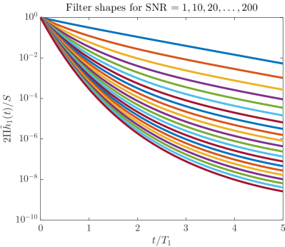
Figure 1: (Color online). The normalized $\mathcal{R}$-optimal filters $2\Pi\tilde{h}_{1}(t)/S$ in log scale versus normalized time $t/T_{1}$ for different input $\textrm{SNR}\equiv S^{2}T_{1}/\Pi=1,10,20,\dots,200$. $\pi_{0}=\pi_{1}=1/2$ and $T=5T_{1}$ are assumed. The different plots can be distinguished by the reducing correlation times for increasing SNR.

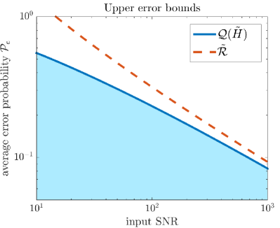
Figure 2: (Color online). Upper bounds $\mathcal{Q}(\tilde{H})$ and $\tilde{\mathcal{R}}$ on the average error probability $\mathcal{P}_{e}$ for the first-order Volterra filter versus input SNR from 10 dB to 30 dB in log-log scale. $\pi_{0}=\pi_{1}=1/2$ and $T=5T_{1}$ are assumed. $\mathcal{P}_{e}$ is guaranteed to be in the shaded region below the curves.

The proposed decision rule can be compared with the optimal likelihood-ratio test (LRT) Van Trees (2001). For the given problem, there exists an analytic expression for the log-likelihood ratio given by Ng and Tsang (2014)

$$\lambda_{o}(y) =\frac{S}{\Pi}\int_{0}^{T}d\eta(t)\check{x}(t)-\frac{S^{2}}{2\Pi}\int_{0}^{T}dt\check{x}^{2}(t),$$ (100)

$$d\eta(t) =y(t)dt,$$ (101)

$$\check{x}(t) =\frac{p_{1}(t)}{p_{0}(t)+p_{1}(t)},$$ (102)

$$p_{1}(t) =\exp\left[\frac{S}{\Pi}\int_{0}^{t}d\eta(\tau)-t\left(\frac{S^{2}}{2\Pi}+\frac{1}{T_{1}}\right)\right],$$ (103)

$$p_{0}(t) =\frac{1}{T_{1}}\int_{0}^{t}d\tau p_{1}(\tau),$$ (104)

where the $d\eta$ integrals are in the Itō sense. The optimal decision rule is thus

$$\lambda_{o}(y)\underset{\mathcal{H}_{0}}{\overset{\mathcal{H}_{1}}{\gtrless}}\ln\frac{\pi_{0}}{\pi_{1}}.$$ (105)

Although the LRT will achieve the lowest $\mathcal{P}_{e}$, the highly nonlinear dependence of $\lambda_{o}$ on $y$ makes its exact implementation difficult in real-time applications or for a large number of qubits.

The average error probabilities for both the $\mathcal{R}$-optimal rule and the LRT are estimated numerically using Monte Carlo simulations and plotted in Fig. 3. The errors are close at lower input SNR values. Considering the simplicity of the $\mathcal{R}$-optimal rule, the divergence at higher SNR is expected and indeed slight. At the input SNR of $10^{3}$, $\mathcal{P}_{e}$ for LRT is $6.2\times 10^{-3}$, while that for the $\mathcal{R}$-optimal rule is only around a factor of 2 higher at $1.48\times 10^{-2}$. A further optimization of $\mathcal{P}_{e}$ beyond the results shown in Fig. 3 can be done by fine-tuning the threshold of the $\mathcal{R}$-optimal rule. For example, a numerical search for the optimal threshold brings its error probability at input SNR $=10^{3}$ down to $8.3\times 10^{-3}$. A higher-order filter is hardly necessary for the SNRs considered here.

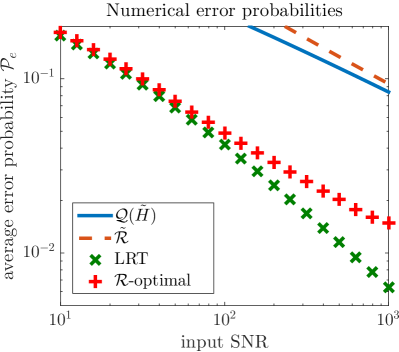
Figure 3: (Color online). Numerically computed average error probabilities $\mathcal{P}_{e}$ for the $\mathcal{R}$-optimal rule and the likelihood-ratio test (LRT) versus the input SNR from 10 dB to 30 dB in log-log scale. $\pi_{0}=\pi_{1}=1/2$ and $T=5T_{1}$ are assumed. Also shown are parts of the upper bounds $\mathcal{Q}(\tilde{H})$ and $\tilde{\mathcal{R}}$ for comparison.

The upper bounds depend only on low-order moments and apply equally to all problems with the same low-order moments, regardless of their higher-order statistics. It is not surprising that such indiscriminate bounds are loose for this particular example, as shown in Fig. 3. What is surprising is the near-optimal performance of a decision rule based on a loose upper bound. The log-likelihood ratio is given analytically for the problem considered here, so one may compare it with the $\mathcal{R}$-optimal test statistic to see how the two resemble each other. In general, however, the log-likelihood ratio is difficult or even impossible to compute if the full probability models are more complicated or simply unidentified. The $\mathcal{R}$-optimal rule requires only low-order moments to be known, and is hence more convenient to implement in practice.

IV Conclusion

I have proposed the use of Volterra filters for quantum estimation and detection. The importance of the proposal lies in its promise to solve many of the practical problems associated with existing optimal quantum inference techniques, including the curse of dimensionality, the lack of performance assurances upon approximations, and the need for a Markovian model. Beyond the examples of quantum state tomography and qubit readout discussed in this paper, diverse applications in quantum information processing Wiseman and Milburn (2010); Nielsen and Chuang (2011); Aspelmeyer et al. (2014), including cooling Steck et al. (2004); *steck06, squeezing Thomsen et al. (2002), state preparation Yanagisawa (2006); *negretti, metrology Helstrom (1976); Holevo (2001); Braginsky and Khalili (1992); Giovannetti et al. (2011); Tsang (2009a); Tsang et al. (2011); Tsang (2012b); *qbzzb; Tsang (2012a); Tsang and Nair (2012); *tsang_open, fundamental tests of quantum mechanics Tsang (2012a, 2013a); Chen (2013); Aspelmeyer et al. (2014), and error correction Ahn et al. (2002); *sarovar; Chase et al. (2008), are expected to benefit. Potential extensions of the theory include adaptive, recursive, and coherent generalizations for feedback control Wiseman and Milburn (2010) and noise cancellation Tsang and Caves (2010); *qmfs; *yamamoto14, filter training via machine learning Hentschel and Sanders (2010); *magesan, robustness analysis, the use of other performance criteria for improved robustness James (2004) or multi-hypothesis testing Tsang (2012a, 2013a), a connection with Shannon information theory through the relations between filtering errors and entropic information Barchielli and Lupieri (2008); *mismatch, and a study of fundamental uncertainty relations in conjunction with quantum lower error bounds Helstrom (1976); Holevo (2001); Giovannetti et al. (2011); Tsang et al. (2011); Tsang and Nair (2012); *tsang_open; Tsang (2012b); *qbzzb.

References

- Wiseman and Milburn (2010) H. M. Wiseman and G. J. Milburn, Quantum Measurement and Control (Cambridge University Press, Cambridge, 2010).
- Gardiner and Zoller (2004) C. W. Gardiner and P. Zoller, Quantum Noise (Springer-Verlag, Berlin, 2004).
- Jacobs (2014) K. Jacobs, Quantum Measurement Theory and its Applications (Cambridge University Press, Cambridge, 2014).
- Bouten et al. (2007) L. Bouten, R. Van Handel, and M. James, SIAM Journal on Control and Optimization 46, 2199 (2007).
- Bouten et al. (2009) L. Bouten, R. van Handel, and M. R. James, SIAM Review 51, 239 (2009).
- Haroche and Raimond (2006) S. Haroche and J. M. Raimond, Exploring the Quantum: Atoms, Cavities, and Photons (Oxford University Press, Oxford, 2006).
- Helstrom (1976) C. W. Helstrom, Quantum Detection and Estimation Theory (Academic Press, New York, 1976).
- Holevo (2001) A. S. Holevo, Statistical Structure of Quantum Theory (Springer-Verlag, Berlin, 2001).
- Braginsky and Khalili (1992) V. B. Braginsky and F. Y. Khalili, Quantum Measurement (Cambridge University Press, Cambridge, 1992).
- Paris and Řeháček (2004) M. G. A. Paris and J. Řeháček, eds., Quantum State Estimation (Springer-Verlag, Berlin, 2004).
- Blume-Kohout (2010) R. Blume-Kohout, New Journal of Physics 12, 043034 (2010).
- Ferrie (2014) C. Ferrie, New Journal of Physics 16, 093035 (2014).
- Riofrío (2014) C. A. Riofrío, Continuous Measurement Quantum State Tomography of Atomic Ensembles, Ph.D. thesis, University of New Mexico, Albuquerque (2014).
- Cook et al. (2014) R. L. Cook, C. A. Riofrío, and I. H. Deutsch, Phys. Rev. A 90, 032113 (2014).
- Audenaert and Scheel (2009) K. M. R. Audenaert and S. Scheel, New Journal of Physics 11, 023028 (2009).
- Six et al. (2015) P. Six, P. Campagne-Ibarcq, I. Dotsenko, A. Sarlette, B. Huard, and P. Rouchon, ArXiv e-prints (2015), arXiv:1510.01726 [quant-ph] .
- Granade et al. (2015) C. Granade, J. Combes, and D. G. Cory, ArXiv e-prints (2015), arXiv:1509.03770 [quant-ph] .
- Giovannetti et al. (2011) V. Giovannetti, S. Lloyd, and L. Maccone, Nature Photon. 5, 222 (2011).
- Tsang (2009a) M. Tsang, Phys. Rev. Lett. 102, 250403 (2009a).
- Tsang (2009b) M. Tsang, Phys. Rev. A 80, 033840 (2009b).
- Tsang (2010) M. Tsang, Phys. Rev. A 81, 013824 (2010).
- Gammelmark et al. (2013) S. Gammelmark, B. Julsgaard, and K. Mølmer, Phys. Rev. Lett. 111, 160401 (2013).
- Guevara and Wiseman (2015) I. Guevara and H. Wiseman, ArXiv e-prints (2015), arXiv:1503.02799 [quant-ph] .
- Tsang (2012a) M. Tsang, Phys. Rev. Lett. 108, 170502 (2012a).
- Tsang (2013a) M. Tsang, Quantum Meas. Quantum Metr. 1, 84 (2013a).
- Gambetta et al. (2007) J. Gambetta, W. A. Braff, A. Wallraff, S. M. Girvin, and R. J. Schoelkopf, Phys. Rev. A 76, 012325 (2007).
- D’Anjou and Coish (2014) B. D’Anjou and W. A. Coish, Phys. Rev. A 89, 012313 (2014).
- D’Anjou et al. (2015) B. D’Anjou, L. Kuret, L. Childress, and W. A. Coish, ArXiv e-prints (2015), arXiv:1507.06846 [quant-ph] .
- Ng and Tsang (2014) S. Ng and M. Tsang, Phys. Rev. A 90, 022325 (2014).
- Wheatley et al. (2010) T. A. Wheatley, D. W. Berry, H. Yonezawa, D. Nakane, H. Arao, D. T. Pope, T. C. Ralph, H. M. Wiseman, A. Furusawa, and E. H. Huntington, Phys. Rev. Lett. 104, 093601 (2010).
- Yonezawa et al. (2012) H. Yonezawa, D. Nakane, T. A. Wheatley, K. Iwasawa, S. Takeda, H. Arao, K. Ohki, K. Tsumura, D. W. Berry, T. C. Ralph, H. M. Wiseman, E. H. Huntington, and A. Furusawa, Science 337, 1514 (2012).
- Iwasawa et al. (2013) K. Iwasawa, K. Makino, H. Yonezawa, M. Tsang, A. Davidovic, E. Huntington, and A. Furusawa, Phys. Rev. Lett. 111, 163602 (2013).
- Belavkin (1989) V. P. Belavkin, Physics Letters A 140, 355 (1989).
- Belavkin (2007) V. P. Belavkin, ArXiv Mathematical Physics e-prints (2007), arXiv:math-ph/0702079 .
- Steck et al. (2004) D. A. Steck, K. Jacobs, H. Mabuchi, T. Bhattacharya, and S. Habib, Phys. Rev. Lett. 92, 223004 (2004).
- Steck et al. (2006) D. A. Steck, K. Jacobs, H. Mabuchi, S. Habib, and T. Bhattacharya, Phys. Rev. A 74, 012322 (2006).
- Thomsen et al. (2002) L. K. Thomsen, S. Mancini, and H. M. Wiseman, Phys. Rev. A 65, 061801 (2002).
- Yanagisawa (2006) M. Yanagisawa, Phys. Rev. Lett. 97, 190201 (2006).
- Negretti et al. (2007) A. Negretti, U. V. Poulsen, and K. Mølmer, Phys. Rev. Lett. 99, 223601 (2007).
- Ahn et al. (2002) C. Ahn, A. C. Doherty, and A. J. Landahl, Phys. Rev. A 65, 042301 (2002).
- Sarovar et al. (2004) M. Sarovar, C. Ahn, K. Jacobs, and G. J. Milburn, Phys. Rev. A 69, 052324 (2004).
- Chase et al. (2008) B. A. Chase, A. J. Landahl, and J. M. Geremia, Phys. Rev. A 77, 032304 (2008).
- Hume et al. (2007) D. B. Hume, T. Rosenband, and D. J. Wineland, Phys. Rev. Lett. 99, 120502 (2007).
- Sayrin et al. (2011) C. Sayrin, I. Dotsenko, X. Zhou, B. Peaudecerf, T. Rybarczyk, S. Gleyzes, P. Rouchon, M. Mirrahimi, H. Amini, M. Brune, J.-M. Raimond, and S. Haroche, Nature (London) 477, 73 (2011).
- Wieczorek et al. (2015) W. Wieczorek, S. G. Hofer, J. Hoelscher-Obermaier, R. Riedinger, K. Hammerer, and M. Aspelmeyer, Phys. Rev. Lett. 114, 223601 (2015).
- Vladimirov and Petersen (2012) I. G. Vladimirov and I. R. Petersen, ArXiv e-prints (2012), arXiv:1202.0946 [quant-ph] .
- Amini et al. (2013) H. Amini, R. A. Somaraju, I. Dotsenko, C. Sayrin, M. Mirrahimi, and P. Rouchon, Automatica 49, 2683 (2013).
- Hush et al. (2013) M. R. Hush, S. S. Szigeti, A. R. R. Carvalho, and J. J. Hope, New Journal of Physics 15, 113060 (2013).
- Nielsen et al. (2009) A. E. B. Nielsen, A. S. Hopkins, and H. Mabuchi, New Journal of Physics 11, 105043 (2009).
- Aspelmeyer et al. (2014) M. Aspelmeyer, T. J. Kippenberg, and F. Marquardt, Rev. Mod. Phys. 86, 1391 (2014).
- Bloch et al. (2008) I. Bloch, J. Dalibard, and W. Zwerger, Rev. Mod. Phys. 80, 885 (2008).
- Houck et al. (2012) A. A. Houck, H. E. Tureci, and J. Koch, Nature Phys. 8, 292 (2012).
- Mathews and Sicuranza (2000) V. J. Mathews and G. L. Sicuranza, Polynomial Signal Processing (Wiley, New York, 2000).
- Tsang et al. (2011) M. Tsang, H. M. Wiseman, and C. M. Caves, Phys. Rev. Lett. 106, 090401 (2011).
- Tsang (2012b) M. Tsang, Phys. Rev. Lett. 108, 230401 (2012b).
- Berry et al. (2015) D. W. Berry, M. Tsang, M. J. W. Hall, and H. M. Wiseman, Phys. Rev. X 5, 031018 (2015).
- Tsang and Nair (2012) M. Tsang and R. Nair, Phys. Rev. A 86, 042115 (2012).
- Tsang (2013b) M. Tsang, New Journal of Physics 15, 073005 (2013b).
- Zhang et al. (2014) J. Zhang, Y.-X. Liu, R.-B. Wu, K. Jacobs, S. Kaya Ozdemir, L. Yang, T.-J. Tarn, and F. Nori, ArXiv e-prints (2014), arXiv:1407.8108 [quant-ph] .
- Belavkin (1994) V. P. Belavkin, Foundations of Physics 24, 685 (1994).
- Gao et al. (2015) Q. Gao, D. Dong, and I. R. Petersen, ArXiv e-prints (2015), arXiv:1504.06780 [math-ph] .
- Ozawa (2003) M. Ozawa, Phys. Rev. A 67, 042105 (2003).
- Bell (1987) J. S. Bell, Speakable and Unspeakable in Quantum Mechanics (Cambridge University Press, Cambridge, 1987).
- Horodecki et al. (2009) R. Horodecki, P. Horodecki, M. Horodecki, and K. Horodecki, Rev. Mod. Phys. 81, 865 (2009).
- Leggett and Garg (1985) A. J. Leggett and A. Garg, Phys. Rev. Lett. 54, 857 (1985).
- Emary et al. (2014) C. Emary, N. Lambert, and F. Nori, Reports on Progress in Physics 77, 016001 (2014).
- Nielsen and Chuang (2011) M. A. Nielsen and I. L. Chuang, Quantum Computation and Quantum Information (Cambridge University Press, Cambridge, 2011).
- Weiss (2008) U. Weiss, Quantum Dissipative Systems (World Scientific, Singapore, 2008).
- Datta (1995) S. Datta, Electronic Transport in Mesoscopic Systems (Cambridge University Press, Cambridge, 1995).
- Bruus and Flensberg (2004) H. Bruus and K. Flensberg, Introduction to Many-Body Quantum Theory in Condensed Matter Physics (Oxford University Press, Oxford, 2004).
- Mandel and Wolf (1995) L. Mandel and E. Wolf, Optical Coherence and Quantum Optics (Cambridge University Press, Cambridge, 1995).
- Berger (1985) J. O. Berger, Statistical Decision Theory and Bayesian Analysis (Springer-Verlag, New York, 1985).
- Van Trees (2001) H. L. Van Trees, Detection, Estimation, and Modulation Theory, Part I. (John Wiley & Sons, New York, 2001).
- Stockton et al. (2002) J. Stockton, M. Armen, and H. Mabuchi, J. Opt. Soc. Am. B 19, 3019 (2002).
- Simon (2006) D. Simon, Optimal State Estimation: Kalman, H Infinity, and Nonlinear Approaches (Wiley, Hoboken, 2006).
- Clerk et al. (2010) A. A. Clerk, M. H. Devoret, S. M. Girvin, F. Marquardt, and R. J. Schoelkopf, Rev. Mod. Phys. 82, 1155 (2010).
- Miao et al. (2015) H. Miao, Y. Ma, C. Zhao, and Y. Chen, ArXiv e-prints (2015), arXiv:1506.00117 [quant-ph] .
- Flammia and Liu (2011) S. T. Flammia and Y.-K. Liu, Phys. Rev. Lett. 106, 230501 (2011).
- Chen (2013) Y. Chen, Journal of Physics B: Atomic, Molecular and Optical Physics 46, 104001 (2013).
- Picinbono and Duvaut (1990) B. Picinbono and P. Duvaut, IEEE Transactions on Information Theory 36, 1061 (1990).
- Picinbono (1995) B. Picinbono, IEEE Transactions on Aerospace and Electronic Systems 31, 1072 (1995).
- Billingsley (1995) P. Billingsley, Probability and Measure (Wiley, New York, 1995).
- Gardiner (2010) C. W. Gardiner, Stochastic Methods: A Handbook for the Natural and Social Sciences (Springer, Berlin, 2010).
- Tsang and Caves (2010) M. Tsang and C. M. Caves, Phys. Rev. Lett. 105, 123601 (2010).
- Tsang and Caves (2012) M. Tsang and C. M. Caves, Phys. Rev. X 2, 031016 (2012).
- Yamamoto (2014) N. Yamamoto, Phys. Rev. X 4, 041029 (2014).
- Hentschel and Sanders (2010) A. Hentschel and B. C. Sanders, Phys. Rev. Lett. 104, 063603 (2010).
- Magesan et al. (2015) E. Magesan, J. M. Gambetta, A. D. Córcoles, and J. M. Chow, Phys. Rev. Lett. 114, 200501 (2015).
- James (2004) M. R. James, Phys. Rev. A 69, 032108 (2004).
- Barchielli and Lupieri (2008) A. Barchielli and G. Lupieri, “Information gain in quantum continual measurements,” in Quantum Stochastics and Information, edited by V. P. Belavkin and M. Guţă (World Scientific, Singapore, 2008) Chap. 15, pp. 325–345, arXiv:quant-ph/0612010 .
- Tsang (2014) M. Tsang, in 2014 IEEE International Symposium on Information Theory (ISIT) (2014) pp. 321–325.