Structured Prediction with Output Embeddings
for Semantic Image Annotation

Abstract

We address the task of annotating images with semantic tuples. Solving this problem requires an algorithm which is able to deal with hundreds of classes for each argument of the tuple. In such contexts, data sparsity becomes a key challenge, as there will be a large number of classes for which only a few examples are available. We propose handling this by incorporating feature representations of both the inputs (images) and outputs (argument classes) into a factorized log-linear model, and exploiting the flexibility of scoring functions based on bilinear forms. Experiments show that integrating feature representations of the outputs in the structured prediction model leads to better overall predictions. We also conclude that the best output representation is specific for each type of argument.

1 Introduction

Many important problems in machine learning can be framed as structured prediction tasks where the goal is to learn functions that map inputs to structured outputs such as sequences, trees or general graphs. A wide range of applications involve learning over large state spaces, i.e., if the output is a labeled graph, each node of the graph may take values over a potentially large set of labels. Data sparsity then becomes a major challenge, as there will be a potentially large number of classes with few training examples.

Within this context, we are interested in the task of predicting semantic tuples for images. That is, given an input image we seek to predict what are the events or actions (predicates), who and what are the participants (actors) of the actions and where is the action taking place (locatives). Fig. 1 shows two examples of the kind of results we obtain. To handle the data sparsity challenge imposed by the large state space, we will leverage an approach that has proven to be useful in multiclass and multilabel prediction tasks [1, 22]. The main idea is to represent a value for an argument $a$ using a feature vector representation $\phi\in I\!\!R^{n}$. We will later describe in more detail the actual representations that we used and how they are computed but for now imagine that we represent an argument by a real vector where each component encodes some particular properties of the argument. We will integrate this argument representation into the structured prediction framework.

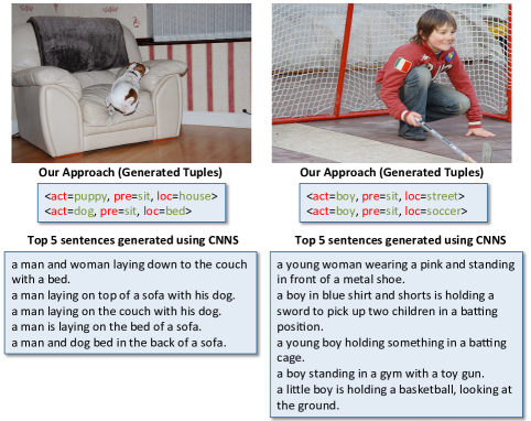
Figure 1: Automatic Tuple Generation. The proposed approach allows generating semantic tuples that have not been jointly observed before. For instance, in the left test image, the joint tuples $\langle puppy,sit,house\rangle$ and $\langle dog,sit,bed\rangle$ are not present in the training set, but our compositional approach can generate them.

More specifically, we consider standard factorized linear models where the score of an input/output pair is the sum of the scores, usually called potentials, of each factor. In our case we will have unary potentials that measure the compatibility between an image and an argument of a tuple, and binary potentials that measure the compatibility between pairs of arguments in a tuple. Typically, both unary and binary potentials are linear functions of some feature representation of the input/output pair. In contrast, we will consider a model that exploits bilinear unary potentials $\phi(y,x)$ of the form $v_{y}^{\intercal}Wx$, where $v_{y}\in I\!\!R^{n}$ is some real vector representation of an argument $l\in L$ and $x\in I\!\!R^{d}$ is a $d$ dimensional feature representation of an image. Similarly, the binary potentials $\alpha(y,y^{\prime})$ will be of the form $v_{y}^{\intercal}Z{v_{y}^{\prime}}$ for a pair of arguments $(y,y^{\prime})$. The rank of $W$ and $Z$ can be interpreted as the intrinsic dimensionality of a low-dimensional embedding of the inputs and arguments feature representation. Thus, if we want computationally efficient models (i.e. few features) it is natural to use the rank of $W$ and $Z$ as a complexity penalty. Since using the rank would lead to a non-convex problem, we use instead the nuclear norm as a convex relaxation. We conduct experiments with two different feature representations of the outputs and show that integrating an output feature representation in the structured prediction model leads to better overall predictions. We also conclude from our results that the best output representation is different for each argument type.

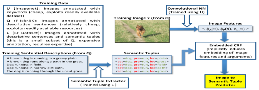
Figure 2: Overview of our approach.

2 Semantic Tuple Image Annotation

2.1 Task

We will address the task of predicting semantic tuples for images. Following [4], we will focus on a simple semantic representation that considers three basic arguments: predicate, actors and locative. For example, an image might be annotated with the semantic tuples: $\langle run,dog,park\rangle$ and $\langle play,dog,grass\rangle$. We call each field of a tuple an argument. For example, in the tuple $t=\langle play,dog,grass\rangle$, “$play$” is the argument of the predicate field, “$dog$” is the actor and “$grass$” the argument of the locative field.

Given this representation, we can formally define our problem as that of learning a function $\theta:~{}X~{}\times~{}P~{}\times~{}A~{}\times~{}L\to I\!\!R$ that scores the compatibility between images and semantic tuples. Here, $X$ is the space of images, $P$ is a discrete set of predicate arguments, $A$ is a set of actor arguments and $L$ is a set of locative arguments. We are particularly interested in cases where $|P|$, $|A|$ and $|L|$ are reasonably large. We will use $T=P\times A\times L$ to refer to the set of possible tuples, and denote by $\langle p\ a\ l\rangle$ a specific instance of the tuple. To learn this function we are provided with a training set $Q$. Each example in this set consists of an image $x$ and a set of corresponding semantic tuples $\{t_{c}\}$ which describe the events occurring in the image. Our goal is to use $Q$ to learn a model for the conditional probability of a tuple given and image. We will use this model to predict semantic tuples for test images by computing the tuples that have highest conditional probability according to our learnt model.

2.2 Dataset

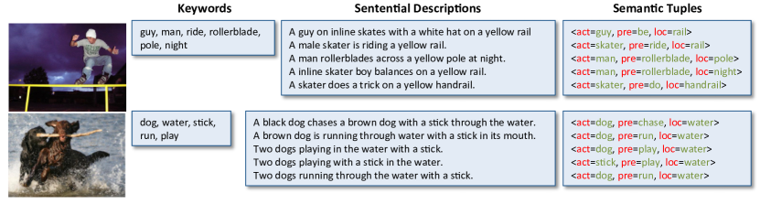
Figure 3: Sample images, keywords, sentences and semantic tuples from the augmented Flickr-8K dataset.

While some datasets of images associated with semantic tuples are already available [4], they only consider small state spaces for each argument type. To address this limitation we decided to create a new dataset of images annotated with semantic tuples. In contrast to previous datasets, we consider a more realistic range of possible argument values. In addition, our dataset has the advantage that every image is annotated with both the underlying semantics in the form of semantic tuples and natural language captions that constitute different lexical realizations of the same underlying semantics. To create our dataset we used a subset of the Flickr8k dataset, proposed in Hodosh et al. [7]. This dataset consists of 8,000 images taken from Flickr of people and animals performing some action, with five crowd-sourced descriptive captions for each one. These captions are sought to be concrete descriptions of what can be seen in the image rather than abstract or conceptual descriptions of non-visible elements (e.g., people or street names, or the mood of the image). This type of language is also known as Visually Descriptive Language [5].

We asked human annotators to annotate 1,544 image captions, corresponding to 311 images (approximately one third of the development set), producing more than 2,000 semantic tuples of predicates, actors and locatives. Annotators were required to annotate every caption with their corresponding semantic tuples without looking at the referent image. We do this to ensure an alignment between the information contained in the captions and their corresponding semantic tuples. Captions are annotated with tuples that consist of a predicate, a patient, an agent and a locative (indeed the patient, the agent and the locative could themselves consist of multiple arguments but for simplicity we regard them as single arguments). For example, the caption “A brown dog is playing and holding a ball in a crowded park” will have the associated tuples: $\langle\ predicate=play,\ agent=dog,\ pacient=null,\ locative=park\rangle$ and $\langle\ predicate=hold,\ agent=dog,\ pacient=ball,\ locative=park\rangle$. Notice that while these annotations are similar to PropBank style semantic role annotations, there are also some differences. First, we do not annotate atomic sentences but captions that might actually consist of multiple sentences. Second, the annotation is done at the highest semantic level and annotators are allowed to make logical inferences to resolve the arguments of a predicate. For example we would annotate the caption: “A man is standing on the street. He is holding a camera” with $\langle\ predicate=standing,\ agent=man,\ pacient=null,\ locative=street\rangle$ and $\langle\ predicate=hold,\ agent=man,\ pacient=null,\ locative=street\rangle$. Figure 3 shows two sample images with captions and annotated semantic tuples. For the experiments we partitioned the set of 311 images (and their corresponding captions and tuples) into a training set of 150 images, a validation set of 50 (used to adjust parameters) and a test set of 100 images.

To enlarge the manually annotated dataset we first used the data of captions paired with semantic tuples to train a model that can predict semantic tuples from image captions. Similar to previous work we start by computing several linguistic features of the captions, ranging from shallow part of speech tags to dependency parsing and semantic role labeling . We extract the predicates by looking at the words tagged as verbs by the POS tagger. Then, the extraction of arguments for each predicate is resolved as a classification problem. More specifically, for each detected predicate in a sentence we regard each noun as a positive or negative training example of a given relation depending on whether the candidate noun is or is not an argument of the predicate. We use these examples to train a discriminative classifier that decides if a candidate noun is or is not an argument of a given predicate in a given sentence. This classifier exploits several linguistic features computed over the syntactic path of the dependency tree connecting the candidate noun and the predicate. As a classifier we trained a linear SVM. We run the learnt tuple predictor model on all the remaining 6,000 training images and corresponding captions of the Ficker8k dataset and produced a larger dataset of images paired with semantic tuples .

3 Incorporating Output Feature Representations into a Factorized Linear Model

For simplicity we will consider factorized sequence models over sequences of fixed length. However, all the ideas we present can be easily generalized to other structured prediction settings. In this section we first describe the general model and learning algorithm (Sections 3.1 and 3.2, respectively), and then, in Section 3.3, we focus on the specific problem of learning tuples given input images.

3.1 Bilinear Models with Output Feature Representations

Let $x$ be an input, and let $y=[y_{1}\ldots y_{T}]$ be some output sequence where $y_{i}\in L$ for some set of states $L$. We are interested in learning a model that computes $P(y|x)$, i.e. the conditional probability of a sequence $y$ given some input $x$. We will consider CRF-like factorized log-linear models that take the form:

$$P(y|x)=\frac{\exp{\theta(x,y)}}{\sum_{y}\exp{\theta(x,y)}}$$ (1)

The scoring function $\theta(x,y)$ is modeled as a sum of unary and binary bilinear potentials and is defined as:

$$\theta(x,y)=\sum_{t=1}^{T}{v_{y_{t}}^{\intercal}W_{t}\phi(x,t)}+\sum_{t=1}^{T}{v_{y_{t}}^{\intercal}Z_{t}v_{y_{t+1}}}$$ (2)

where $v_{y}\in I\!\!R^{|n|}$ is a feature representation of label $y\in L$, and $\phi(x,t)\in I\!\!R^{d}$ is a feature representation of the $t$-th input factor of $x$.

The first set of terms in the above equation are usually refered as unary potentials and measure the compatibility between a single state at $t$ and the feature representation of input factor $t$. The second set of terms are the binary potentials and measure the compatibility between pairs of states at adjacent factors. The scoring function $\theta(x,y)$ is fully parameterized by the unary parameter matrices $W\in I\!\!R^{|n|\times d}$ and the binary parameter matrices $Z\in I\!\!R^{|n|\times|n|}$.

We will later describe the actual label feature representations that we used in our experiments. But for now, it suffices to say that the main idea is to define a feature space so that semantically similar labels will be close in that space. Like in the multilabel scenario [1, 22], having full feature representations for arguments will allow us to share information across different classes.

One of the most important advantages of using feature representations for the outputs is that they give us the ability to generalize better. This is because with a good output feature representation, our model should be able to make sensible predictions about pairs of arguments that were not observed at training. This is easy to see: consider a case were we have a pair of arguments represented with feature vectors $a_{1}$ and $a_{2}$ and suppose that we have not observed the factor $a_{1},a_{2}$ in our training data but we have observed the factor $b_{1},b_{2}$. Then if $a_{1}$ is close in the feature space to argument $b_{1}$ and $a_{2}$ is close to $b_{2}$ our model will predict that $a_{1}$ and $a_{2}$ are compatible. That is, it will assign probability to the pair of arguments $a_{1},a_{2}$ which seems a natural generalization from the observed training data.

This kind of representation also has interesting interpretations in terms of the ranks of $W$ and $Z$. Let $W=U\Sigma V$ be the singular value decomposition of $W$. We can then write the unary potential $v_{y}^{\intercal}W\phi(x,t)$ as:

$$v_{y}^{\intercal}U\ \Sigma\ [V\phi(x,t)].$$ (3)

Thus, we can regard the bilinear form as a function computing a weighted inner product between some real embedding $v_{y}^{\intercal}U$ representing state $y$, and some real embedding $[V\phi(x,t)]$ representing input factor $t$. The rank of $W$ gives us the intrinsic dimensionality of the embedding. Therefore, if we seek to induce shared low-dimensional embeddings across different states it seems reasonable to impose a low rank penalty on $W$.

Similarly, let $Z=U\Sigma V$ be the singular value decomposition of $Z$. We can write the binary potentials $v_{y}^{\intercal}Zv_{y^{\prime}}$ as:

$$v_{y}^{\intercal}U\ \Sigma\ Vv_{y^{\prime}}$$ (4)

and thus the binary potentials compute a weighted inner product between a real embedding of state $y$ and a real embedding of state $y^{\prime}$. Again, the rank of $Z$ gives us the intrinsic dimensionality of the embedding and, to induce a low dimensional embedding for binary potentials, we will impose a low rank penalty on $Z$. In practice, imposing low-rank constraints, would lead to a hard optimization problem, so instead we will use the nuclear norm as a convex relaxation of the rank function.

3.2 Learning Algorithm

Inputs: $D,\eta,\gamma,c$

Output: $W$

Initialize $W=0$

while $t\leq MaxIter$ do

       $G_{t}=\partial(Loss(D,\{W\}))/\partial{W}$;

       $W_{t+0.5}=W_{t}-\nu_{t}G_{t}$; // $\nu_{t}$ is the learning rate

       $W_{t+0.5}=U\Sigma V^{\intercal}$;

       $\forall$ unary potentials define a diagonal matrix $\Sigma^{\prime}$ such that: $\sigma_{i}^{\prime}=\max[\sigma_{i}-\nu_{t}\eta]$;

       $W_{t+1}=U\Sigma^{\prime}V^{\intercal}$;

       $\forall$ binary potentials define a diagonal matrix $\Sigma^{\prime}$ such that: $\sigma_{i}^{\prime}=\max[\sigma_{i}-\nu_{t}\gamma]$;

       $W_{t+1}=U\Sigma^{\prime}V^{\intercal}$;

end while

Algorithm 1 Learning Algorithm

After having described the type of scoring functions we are interested in, we now turn our attention to the learning problem. That is, given a training set $D=\{\langle x\ y\rangle\}$ of pairs of inputs $x$ and output sequences $y$ we need to learn the parameters $\{W\}$ and $\{Z\}$. For this purpose we will do standard max-likelihood estimation and find the parameters that minimize the conditional negative log-likelihood of the data in $D$. That is, we will find the $\{W\}$ and $\{Z\}$ that minimize the following loss function $Loss(D,\{W\},\{Z\}$):

$$-\sum_{\langle x\ y\rangle\in D}\log P(y|x;\{W\},\{Z\})$$

It can be shown that this loss function is convex on $\{W\}$ and $\{Z\}$ whenever $\theta(x,t;\{W\},\{Z\})$ is convex, which is the case for our scoring function.

Recall that we are interested in learning low-rank unary and binary potentials. To this end we follow the standard approach which is to use the nuclear norm $|W|_{*}$ and $|Z|_{*}$ (i.e. the $l_{1}$ norm of the singular values) as a convex approximation of the rank function. Putting all this together, the final optimization problem becomes:

$$\min_{\{W\}}Loss(D,\{W\})+c_{1}\sum_{t}|W_{t}|_{*}+c_{2}\sum_{t}|Z_{t}|_{*}$$ (5)

where $Loss(D,\{W\})=\sum_{d\in D}Loss(d,\{W\})$ is the negative log likelihood function and $c_{1}$ and $c_{2}$ are two constants that control the trade off between minimizing the loss and the implicit dimensionality of the embeddings.

In recent years, many algorithms have been proposed for optimizing trace norm regularized problems (e.g., see [8, 17, 9]). We use a simple optimization scheme known as Forward Backward Splitting, or FOBOS [3]. It can be shown that FOBOS converges to the global optimum at a $O(1/\epsilon^{2})$ rate.

The main steps of the optimization involve computing the gradient of the loss function and performing singular value decomposition on each $W$ and $Z$. In our case, computing the gradient involves computing marginal probabilities for unary and binary potentials which has a cost of $O(|L|^{2})$ and the cost of the SVD computation for each $W$ in $\{W\}$ and each $Z$ in $\{Z\}$.

3.3 Bilinear CRF for Predicate Prediction

For our task we will consider a simple factorized scoring function $\theta(x,\langle p\ a\ l\rangle)$ that has unary terms relating arguments of the same kind, and binary factors associated with the $locative-predicate$ pair and with the $predicate-actor$ pair. Since this corresponds to a chain structure, $\arg\max_{t\in T}\theta(x;\langle p\ a\ l\rangle)$ can be efficiently computed using Viterbi decoding in time $O(N^{2})$, where $N=\max(|P|,|A|,|L|)$. Similarly, we can also find the top $k$ predictions in $O(kN^{2})$. Alternatively, we could have defined the relationship between arguments via a fully connected graph and use approximate inference methods.

More specifically, the scoring function of the bilinear CRF we contemplate takes the form:

$$\theta(x,\langle p\ a\ l\rangle) = \lambda_{loc}(l)^{\intercal}W_{loc}\phi_{loc}(l)$$ (6)

$$+\lambda_{pre}(p)^{\intercal}W_{pre}\phi_{pre}(p)$$

$$+\lambda_{act}(a)^{\intercal}W_{act}\phi_{act}(a)$$

$$+\phi_{loc}(l)^{\intercal}W^{loc}_{pre}\phi_{pre}(p)$$

$$+\phi_{pre}(p)^{\intercal}W^{pre}_{act}\phi_{act}(a)$$

where the $\lambda$’s are the image representations and the $\phi$’s the textual ones. The unary potentials (first three terms in Eq. 6) measure the compatibility between image and semantic arguments; the first binary potential measures the compatibility between the semantic representations of locatives and predicates, and the second binary potential measures the compatibility between predicates and actors. The scoring function is fully parameterized by the unary parameter matrices $W_{loc}\in I\!\!R^{d\times nl}$, $W_{pre}\in I\!\!R^{d\times np}$ and $W_{a}\in I\!\!R^{d\times na}$ and by the binary parameter matrices $W^{loc}_{pre}\in I\!\!R^{nl\times np}$ and $W^{pre}_{act}\in I\!\!R^{np\times na}$. The parameters $nl$, $np$ and $na$ are the dimensionalities of feature representations for the locatives, predicates and actors.

Note that if we let the argument representation $\phi(r)$ be an indicator vector in $I\!\!R^{|L|}$ we obtain the usual parametrization of a standard factorized linear model:

$$\theta(x,\langle p\ a\ l\rangle) = \lambda_{loc}(l)^{\intercal}w_{loc}^{l}$$

$$+\lambda_{pre}(p)^{\intercal}w_{pre}^{p}$$

$$+\lambda_{act}(a)^{\intercal}w_{act}^{a}$$

$$+W^{loc}_{pred}(l,p)+W^{pred}_{act}(p,a)$$

Like in the multilabel scenario [1, 22], having full feature representations for arguments instead of indicator vectors will allow us to share information across different classes. In fact, we will use the model that uses indicator vectors as a baseline in our experiments.

4 Representing Semantic Arguments

Recall that in order to handle the large number of possible arguments per field (i.e. data sparsity) our model assumes the existence of some feature representation for each argument and type $\phi_{pred}(p)\in I\!\!R^{np}$, $\phi_{act}(a)\in I\!\!R^{na}$ and $\phi_{loc}\in I\!\!R^{nl}$. It is then that by learning an embedding of these vectors we will be able to share information across different classes. Intuitively, the feature vectors should describe properties of the arguments and should be defined so that feature vectors that are close to each other represent arguments that are semantically similar.

We will conduct experiments with two different feature representations: 1) Fully unsupervised Skip-Gram based Continuous Word Representations (SCWR) and 2) a feature representation computed using the $\langle caption,semantic-tuples\rangle$ pairs, that we call Semantic Equivalence Representation (SER). We next describe in more detail each of these representations.

4.1 Semantic Equivalence Representation

We want to exploit the dataset of captions paired with semantic tuples to induce a useful feature representation for arguments. For this we will propose a way to illustrate the fact that any pair of semantic tuples associated with the same image will likely be describing the same event. Thus, they are in essence different ways of lexicalizing the same underlying concept.

Let’s look at a concrete example. Imagine that we have an image annotated with the tuples: $\langle play,\ dog,\ water\rangle$ and $\langle play,\ dog,\ river\rangle$. Since both tuples describe the same image, it is quite likely that both “$river$” and “$water$” refer to the same real world entity, i.e, “$river$” and “$water$” are ’semantically equivalent’ for this image. Using this idea we build a representation $\phi_{loc}(i)\in I\!\!R^{|L|}$ where the $j$-th dimension corresponds to the number of times the argument $j$ has been semantically equivalent to argument $i$.

More precisely, we compute the probability that argument $j$ can be exchanged with argument $i$ as: $\frac{[i,j]_{sr}}{\sum_{j}[i,j]_{sr}}$, where $[i,j]_{sr}$ is the number of times that $i$ and $j$ have appeared as annotations of the same image and with the same other arguments. For example, for the actor arguments $[i,j]_{sr}$ represents the number of time that actor $i$ and actor $j$ have appeared with the same locative and predicate as descriptions of the same image. Here is a concrete example of the feature vector for the locative ‘water’ (we report the non-zero dimensions and their corresponding value): $\phi_{loc}(water)$=[ air 0.03, beach 0.06, boat 0.03, canoe 0.03, dock 0.13, grass 0.06, kayak 0.06, lake 0.06, mud 0.03, ocean 0.16, platform 0.03, pond 0.06, puddle 0.1, rock 0.03, snow 0.03, tree 0.03, waterfall 0.03]. Thus, according to the computed representation, ‘water’ is semantically most similar to ‘ocean’.

4.2 Skip-Gram based Continuous Word Representations

Recently, there has been interest in learning word-representations, which have been proven to be useful for many structure prediction tasks [20, 12, 19]. We use continuous word representations (also known as distributed representations) to tailor a task-specific embedding. Continuous word representations consist of neural network-based low-dimensional real valued vectors of each word. We use [15]’s skip-gram based approach for inducing continuous word representations. Skip-gram based representations are essentially a single layer neural network, and are based on inner products between two word vectors. The objective function in a skip-gram is to predict a word’s context given the word itself. We use the trained continuous word representations computed over the Google News dataset(100 billion words), that is publicly available, in our experiments.

5 Related Work

In recent years, some works have tackled the problem of generating rich textual descriptions of images. One of the pioneers is [13], where a CRF model combines the output of several vision systems to produce input for a language generation method. This seminal work, however, only considered a limited set of a few tens of labels, while we aim at dealing with potentially hundreds of labels simultaneously. In [4], the authors find the similarity between sentences and images in a “meaning” space, represented by semantic tuples which are very similar to ours: triplets of object, action and scene. The main difference with this work is that it uses a ruled based system to extract semantic tuples from dependency trees where we train a model that predicts semantic tuples and, most importantly, it uses a standard factorized linear model while we propose a model that leverages feature representations of arguments, and can therefore handle significantly larger state spaces.

Other works focus on the simplified problem of ranking human-generated captions for images. In [7] the authors propose to use Kernel Canonical Correlation Analysis to project images and their captions into a joint representation space, in which images and captions can be related and ranked to perform illustration and annotation tasks. However, the system cannot be used to generate novel image descriptions for new images and, since a kernel is necessary, it has limitations on the number of image/caption pairs that can be used to define the subspace. In a follow-up work, the authors address improving the text/image embeddings with abundant weakly-annotated data from Flickr and similar sites using a stacked representation [6]. To cope with the large amounts of data, Normalized Canonical Correlation Analysis is used. Socher et al. [18] also address the ranking of images given a sentence and vice-versa using a common subspace, also known as zero-shot learning. Recursive Neural Networks are used to learn this common representation. The work of [14] performs natural text generation from images using a bank of detectors to find objects and compressing the text to retrieve ‘generalizable’ small fragments. On top of this, a tree approach is used to construct sentences given the observations and fragments. However, the sentences produced this way can be easily corrupted by wrongly retrieved segments.

Recent works use deep networks to address the problem: [21] propose a pure deep network approach, where convolutional neural networks are used both to extract image features and recursive deep network to generate the text. The system is trained to maximize likelihood end-to-end. [11] use a common multi-modal embedding to align text and images, and a recurrent neural network is trained to generate sentences directly from the image pixels. Although these methods report good results in terms of BLEU score agreement with gold captions, they do not model the underlying visual predicates which is the goal of this paper.

Using label embeddings and its combination with bilinear forms has been previously proposed in the context of multiclass and multilabel image classification [1, 22], but to the best of our knowledge there is no previous work on leveraging output embeddings in the context of structured prediction. Thus, besides the concrete application to semantic tuple image generation, this paper presents a useful modeling tool for handling structured prediction problems in large state spaces. Our model can be used whenever we have some means of computing a feature representation of the outputs.

6 Experiments

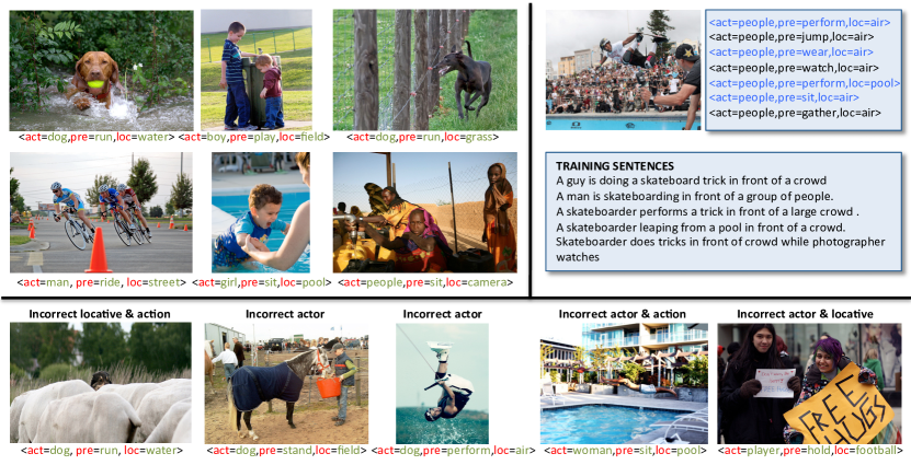
Figure 4: Samples of predicted tuples. Top-left: Examples of visually correct predictions. Bottom: Typical errors on one or several arguments. Top-right: Sample image and its top predicted tuples. The tuples in blue were not observed neither in the SP-Dataset nor in the automatically enlarged dataset. Note that all of them are descriptive of what is occurring in the scene.

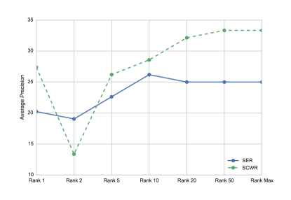
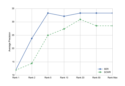
Figure 5: Performance as a function of the size of the intrinsic embedded space for predicate (left) and locative (right) arguments.

As it is standard practice, in order to compute image representations ($\lambda$-vectors in Eq.6), we use the 4,096-dimensional second to last layer of a Convolutional Neural Network (CNN). The full network has 5 convolutional layers followed by 3 fully connected layers, and obtained the best performance in the ILSVRC-2012 challenge. The network is trained on a subset of ImageNet [2] to classify 1,000 different classes and we use the publicly available implementation and pre-trained model provided by [10]. The features obtained with this procedure have been shown to generalize well and outperform traditional hand-crafted features, thus they are already being used in a wide diversity of tasks [18, 23].

To test our method we used the 100 test images that were annotated with ground-truth semantic tuples. For locatives, predicates and actors we consider the 400 most frequent. To measure performance we first compute the top 5 tuples for each image. Then, we define the set of predicted locatives to be the union of all predicted locatives and we do the same for the other argument types. Finally, we compute the precision for each type, for example, for the locatives this is the percentage of predicted locatives that were present in the gold tuples for the corresponding image.

The regularization parameters of each model were set using the validation set. We compare the performance of several models:

• Baseline KCCA: This model implements the Kernel Canonical Correlation Analysis approach of [7]. We first note that this approach is able to rank a list of candidate captions but cannot directly generate tuples. To generate tuples for test images we first find the caption in the training set that has the highest ranking score for that image and then extract the corresponding semantic tuples from that caption. These are the tuples that we consider as predictions of the KCCA model.

• Baseline Separate Predictors (SPred): We also consider a baseline made of independent predictors for each argument type. More specifically we train one-vs-all SVMs (we also tried multi-class SVMs but they did not improve performance) to independently predict locatives, predicates and actors. For each argument type and candidate label we have a score computed by the corresponding SVM. Given an image we generate the top tuples that maximize the sum of scores for each argument type.

• Embedded CRF with Indicator Features (IND), this is a standard factorized log-linear model that does not use any feature representation for the outputs.

• Embedded CRF with a model that uses the skip-gram continuous word representation of outputs (SCWR).

• Embedded CRF with a model that uses that semantic equivalence representation of outputs (SER).

• A combined model that makes predictions using the best feature representation for each argument type (COMBO).

Table 1 reports the results for the baselines and of the different CRF schemes. The first observation is that the best performing output feature representation is different for each argument type. For the locatives the best representation is SER, for the predicates is the SCWR and for the actors using an output feature representation causes a drop in performance. The largest improvement from using an output feature representation that we obtain is on the predicate arguments, where we improve almost by 10% over the indicator representation by using the skip-gram representation. Overall, the model that uses the best representation performs better than the indicator baseline.

Finally, Figure 5 shows performance as a function of the dimensionality of the learnt embedding, i.e. rank of parameter matrices, as we can see the learnt models are efficient in the sense that they can work well with low-dimensional projections of the features.

	Spred	KCCA	IND	SCWR	SER	COMBO
LOC	15	23	32	28	33
PRED	11	20	24	33	25
ACT	30	25	52	51	50
MEAN	18.6	22.6	36	37.3	36	39.3

Table 1: Precision of baseline and CRFs with different output embeddings.

7 Conclusion

In this paper we have presented a model for exploiting input and output embeddings in the context of structured prediction. We have applied this framework to the problem of predicting compositional semantic descriptions of images. Our results show the advantages of using output embeddings for handling large state spaces. We have also seen that regularizing with the nuclear norm we can obtain computationally efficient low-rank models with comparable performance.

References

- [1] Z. Akata, F. Perronnin, Z. Harchaoui, and C. Schmid. Label-embedding for attribute-based classification. In Proc. IEEE Conference on Computer Vision and Pattern Recognition (CVPR), 2013.
- [2] J. Deng, W. Dong, R. Socher, L.-J. Li, K. Li, and L. Fei-Fei. ImageNet: A Large-Scale Hierarchical Image Database. In Proc. IEEE Conference on Computer Vision and Pattern Recognition (CVPR), 2009.
- [3] J. Duchi and Y. Singer. Efficient online and batch learning using forward backward splitting. Journal of Machine Learning Research (JMLR), 10:2899–2934, 2009.
- [4] A. Farhadi, M. Hejrati, M. Sadeghi, P. Young, C. Rashtchian, J. Hockenmaier, and D. Forsyth. Every picture tells a story: Generating sentences from images. In Proc. European Conference on Computer Vision (ECCV). 2010.
- [5] R. Gaizauskas, J. Wang, and A. Ramisa. Defining visually descriptive language. In Proceedings of the 2015 Workshop on Vision and Language (VL’15): Vision and Language Integration Meets Cognitive Systems, 2015.
- [6] Y. Gong, L. Wang, M. Hodosh, J. Hockenmaier, and S. Lazebnik. Improving image-sentence embeddings using large weakly annotated photo collections. In eccv, pages 529–545. Springer, 2014.
- [7] M. Hodosh, P. Young, and J. Hockenmaier. Framing image description as a ranking task: Data, models and evaluation metrics. Journal of Artificial Intelligence Research (JAIR), 47:853–899, 2013.
- [8] M. Jaggi and M. Sulovský. A simple algorithm for nuclear norm regularized problems. In International Conference on Machine Learning (ICML), 2010.
- [9] S. Ji and J. Ye. An accelerated gradient method for trace norm minimization. In International Conference on Machine Learning (ICML), 2009.
- [10] Y. Jia. Caffe: An open source convolutional architecture for fast feature embedding. http://caffe.berkeleyvision.org/, 2013.
- [11] A. Karpathy and L. Fei-Fei. Deep visual-semantic alignments for generating image descriptions. In Proc. IEEE Conference on Computer Vision and Pattern Recognition (CVPR), 2015.
- [12] T. Koo, X. Carreras, and M. Collins. Simple semi-supervised dependency parsing. ACL-08: HLT, page 595, 2008.
- [13] G. Kulkarni, V. Premraj, S. Dhar, S. Li, Y. Choi, A. C. Berg, and T. L. Berg. Baby talk: Understanding and generating image descriptions. In Proc. IEEE Conference on Computer Vision and Pattern Recognition (CVPR), 2011.
- [14] P. Kuznetsova, V. Ordonez, T. Berg, and Y. Choi. Treetalk: Composition and compression of trees for image descriptions. Transactions of the Association for Computational Linguistics, 2014.
- [15] T. Mikolov, K. Chen, G. Corrado, and J. Dean. Efficient estimation of word representations in vector space. arXiv preprint arXiv:1301.3781, 2013.
- [16] L. Padro and E. Stanilovsky. Freeling 3.0: Towards wider multilinguality. In Proc. Language Resources and Evaluation Conference (LREC), 2012.
- [17] S. Shalev-Shwartz, Y. Singer, N. Srebro, and A. Cotter. Pegasos: primal estimated sub-gradient solver for svm. Mathematical Programming, 127(1):3–30, 2011.
- [18] R. Socher, A. Karpathy, Q. V. Le, C. D. Manning, and A. Y. Ng. Grounded compositional semantics for finding and describing images with sentences. Transactions of the Association of Computational Linguistics (TACL), 2:207–218, 2014.
- [19] O. Täckström, R. McDonald, and J. Uszkoreit. Cross-lingual word clusters for direct transfer of linguistic structure. In Proceedings of the 2012 Conference of the North American Chapter of the Association for Computational Linguistics: Human Language Technologies, pages 477–487. Association for Computational Linguistics, 2012.
- [20] J. Turian, L. Ratinov, and Y. Bengio. Word representations: a simple and general method for semi-supervised learning. In Proceedings of the 48th annual meeting of the association for computational linguistics, pages 384–394. Association for Computational Linguistics, 2010.
- [21] O. Vinyals, A. Toshev, S. Bengio, and D. Erhan. Show and tell: A neural image caption generator. In Proc. IEEE Conference on Computer Vision and Pattern Recognition (CVPR), 2015.
- [22] J. Weston, S. Bengio, and N. Usunier. Large scale image annotation: Learning to rank with joint word-image embeddings. In Proc. European Conference on Computer Vision (ECCV), 2010.
- [23] J. Xu, A. G. Schwing, and R. Urtasun. Tell me what you see and i will show you where it is. In Proc. IEEE Conference on Computer Vision and Pattern Recognition (CVPR), 2014.