Fermion and scalar phenomenology of a 2-Higgs doublet model with S3subscript𝑆3S_{3}

A. E. Cárcamo Hernández antonio.carcamo@usm.cl Universidad Técnica Federico Santa María and Centro Científico-Tecnológico de Valparaíso
Casilla 110-V, Valparaíso, Chile
   I. de Medeiros Varzielas ivo.de@soton.ac.uk School of Physics and Astronomy, University of Southampton,
Southampton, SO17 1BJ, U.K.
   E. Schumacher erik.schumacher@tu-dortmund.de Fakultät für Physik, Technische Universität Dortmund
D-44221 Dortmund, Germany
Abstract

We propose a 2-Higgs doublet model where the symmetry is extended by S3Z3Z3Z14tensor-productsubscript𝑆3subscript𝑍3superscriptsubscript𝑍3subscript𝑍14S_{3}\otimes Z_{3}\otimes Z_{3}^{\prime}\otimes Z_{14} and the field content is enlarged by extra SU(2)L𝑆𝑈subscript2𝐿SU(2)_{L} singlet scalar fields. S3subscript𝑆3S_{3} makes the model predictive and leads to viable fermion masses and mixing. The observed hierarchy of the quark masses arises from the Z3superscriptsubscript𝑍3Z_{3}^{\prime} and Z14subscript𝑍14Z_{14} symmetries. The light neutrino masses are generated through a type I seesaw mechanism with two heavy Majorana neutrinos. In the lepton sector we obtain mixing angles that are nearly tri-bi-maximal, in an excellent agreement with the observed lepton parameters. The vacuum expectation values required for the model are naturally obtained from the scalar potential, and we analyze the scalar sector properties further constraining the model through rare top decays (like tch𝑡𝑐t\to ch), the hγγ𝛾𝛾h\to\gamma\gamma decay channel and the T𝑇T and S𝑆S parameters.

preprint: DO-TH 15/12

I Introduction

The flavor puzzle is not understood in the context of the Standard Model (SM), which does not specify the Yukawa structures and has no justification for the number of generations. As such, extensions addressing the fermion masses and mixing are particularly appealing. With neutrino experiments increasingly constraining the mixing angles in the leptonic sector many models focus only on this sector, aiming to explain the near tri-bi-maximal structure of the PMNS matrix through some non-Abelian symmetry.

Discrete flavor symmetries have shown a lot of promise and S3subscript𝑆3S_{3}, as the smallest non-Abelian group has been considerably studied in the literature since Pakvasa:1977in , with interesting results for quarks, leptons or both, and remains a popular group Cardenas:2012bg ; Dias:2012bh ; Dev:2012ns ; Meloni:2012ci ; Canales:2013cga ; Ma:2013zca ; Kajiyama:2013sza ; Hernandez:2013hea ; Hernandez:2014lpa ; Hernandez:2014vta ; Vien:2014vka ; Ma:2014qra ; Das:2014fea ; Das:2015sca . Other popular groups are the smallest groups with triplet representations, particularly A4subscript𝐴4A_{4} which has only a triplet and three distinct singlets. A4subscript𝐴4A_{4} was used in Ma:2001dn ; Babu:2002dz ; Altarelli:2005yp ; Altarelli:2005yx ; deMedeirosVarzielas:2005qg and more recently in Varzielas:2012ai ; Ishimori:2012fg ; Ahn:2013mva ; Memenga:2013vc ; Bhattacharya:2013mpa ; Ferreira:2013oga ; Felipe:2013vwa ; Hernandez:2013dta ; King:2013hj ; Morisi:2013qna ; Morisi:2013eca ; Felipe:2013ie ; Campos:2014lla ; Hernandez:2015tna ; Pramanick:2015qga . With just triplets and singlet representations the groups T7subscript𝑇7T_{7} Luhn:2007sy ; Hagedorn:2008bc ; Cao:2010mp ; Luhn:2012bc ; Kajiyama:2013lja ; Bonilla:2014xla ; Hernandez:2015cra ; Arbelaez:2015toa and Δ(27)Δ27\Delta(27) deMedeirosVarzielas:2006fc ; Ma:2006ip ; Varzielas:2012nn ; Bhattacharyya:2012pi ; Ma:2013xqa ; Varzielas:2013sla ; Aranda:2013gga ; Varzielas:2013eta ; Varzielas:2015aua are also promising as flavor symmetries. For recent reviews on the use of discrete flavor groups, see Refs. King:2013eh ; King:2014nza .

In this work we make use of the S3subscript𝑆3S_{3} group to formulate a 2-Higgs doublet model (2HDM) with an extra S3Z3Z3Z14tensor-productsubscript𝑆3subscript𝑍3superscriptsubscript𝑍3subscript𝑍14S_{3}\otimes Z_{3}\otimes Z_{3}^{\prime}\otimes Z_{14} symmetry. Assigning the SM fermions under this symmetry and using scalars transforming under the different irreducible representations of S3subscript𝑆3S_{3}, we provide an existence proof of models leading to the viable mixing inspired quark textures presented in Hernandez:2014zsa , by building a minimal realization. We then consider the model in the lepton sector where we obtain viable masses and mixing angles by using assignments that lead to a charged lepton texture similar to that of the down-type quarks, with the neutrino sector being completed through a type I seesaw. We discuss the scalar potential in some detail, showing it leads to the Vacuum Expectation Values (VEVs) used to obtain the fermion masses, and analyzing phenomenological processes that constrain the parameters of the model such as tch𝑡𝑐t\to ch and hγγ𝛾𝛾h\to\gamma\gamma.

The paper is outlined as follows. In Section II we describe the field and symmetry content of the model, including a brief revision of the quark mass and mixing angles presented in Hernandez:2014zsa (Section II.1) and the equivalent analysis for the lepton sector (Section II.2). Section III contains the analysis of the phenomenology associated with the extended scalar sector, presenting the Yukawa couplings, an analysis of rare top decays, then considering the hγγ𝛾𝛾h\to\gamma\gamma rate (Section III.1) and the T𝑇T and S𝑆S parameters (Section III.2). We present our conclusions in Section IV. We relegate some technical discussions that are relevant for the paper to the Appendix.

II The Model

We consider an extension of the SM with extra scalar fields and discrete symmetries, which reproduces the predictive mixing inspired textures proposed in Ref. Hernandez:2014zsa , i.e. the Cabbibo mixing arises from the down-type quark sector whereas the up-type quark sector contributes to the remaining mixing angles. These textures describe the charged fermion masses and quark mixing pattern in terms of different powers of the Wolfenstein parameter λ=0.225𝜆0.225\lambda=0.225 and order one parameters. Because of the required mismatch between the down-type quark and up-type quark textures, to obtain these textures in a model we use two Higgs doublets distinguished by a symmetry (in our model, a Z3subscript𝑍3Z_{3}). In the following, we describe our 2HDM with the inclusion of the S3Z3Z3Z14tensor-productsubscript𝑆3subscript𝑍3superscriptsubscript𝑍3subscript𝑍14S_{3}\otimes Z_{3}\otimes Z_{3}^{\prime}\otimes Z_{14} discrete symmetry and four singlet scalar fields, assigned in a S3subscript𝑆3S_{3} doublet, one S3subscript𝑆3S_{3} trivial singlet and one S3subscript𝑆3S_{3} non trivial singlet. We use the S3subscript𝑆3S_{3} discrete group since it is the smallest non-Abelian group, having a doublet and two singlets as irreducible representations. The full symmetry 𝒢𝒢\mathcal{G} of the model is broken spontaneously in two steps:

𝒢=SU(3)CSU(2)LU(1)YS3Z3Z3Z14𝒢tensor-producttensor-producttensor-product𝑆𝑈subscript3𝐶𝑆𝑈subscript2𝐿𝑈subscript1𝑌subscript𝑆3subscript𝑍3superscriptsubscript𝑍3subscript𝑍14\displaystyle\mathcal{G}=SU(3)_{C}\otimes SU(2)_{L}\otimes U\left(1\right)_{Y}\otimes S_{3}\otimes Z_{3}\otimes Z_{3}^{\prime}\otimes Z_{14} (1)
ΛabsentΛ\displaystyle\hskip 99.58464pt\Downarrow\Lambda
SU(3)CSU(2)LU(1)YZ3tensor-producttensor-producttensor-product𝑆𝑈subscript3𝐶𝑆𝑈subscript2𝐿𝑈subscript1𝑌subscript𝑍3\displaystyle\hskip 42.67912ptSU\left(3\right)_{C}\otimes SU\left(2\right)_{L}\otimes U\left(1\right)_{Y}\otimes Z_{3}
ΛEWabsentsubscriptΛ𝐸𝑊\displaystyle\hskip 99.58464pt\Downarrow\Lambda_{EW}
SU(3)CU(1)em,tensor-product𝑆𝑈subscript3𝐶𝑈subscript1𝑒𝑚\displaystyle\hskip 65.44133ptSU\left(3\right)_{C}\otimes U\left(1\right)_{em},

where the different symmetry breaking scales satisfy the following hierarchy ΛΛEWmuch-greater-thanΛsubscriptΛ𝐸𝑊\Lambda\gg\Lambda_{EW}, where ΛEW=246subscriptΛ𝐸𝑊246\Lambda_{EW}=246 GeV is the electroweak symmetry breaking scale.

Field q1Lsubscript𝑞1𝐿q_{1L} q2Lsubscript𝑞2𝐿q_{2L} q3Lsubscript𝑞3𝐿q_{3L} URsubscript𝑈𝑅U_{R} u3Rsubscript𝑢3𝑅u_{3R} d1Rsubscript𝑑1𝑅d_{1R} d2Rsubscript𝑑2𝑅d_{2R} d3Rsubscript𝑑3𝑅d_{3R} l1Lsubscript𝑙1𝐿l_{1L} l2Lsubscript𝑙2𝐿l_{2L} l3Lsubscript𝑙3𝐿l_{3L} l1Rsubscript𝑙1𝑅l_{1R} l2Rsubscript𝑙2𝑅l_{2R} l3Rsubscript𝑙3𝑅l_{3R} ν1Rsubscript𝜈1𝑅\nu_{1R} ν2Rsubscript𝜈2𝑅\nu_{2R}
S3subscript𝑆3S_{3} 1 1 1 2 1 1 1 1 1 1 1 1’ 1 1 1 1
Z3subscript𝑍3Z_{3} 0 0 1 0 1 2 2 1 2 0 0 1 0 0 0 0
Z3superscriptsubscript𝑍3Z_{3}^{\prime} 0 0 0 0 0 0 0 0 0 0 0 2 0 0 0 0
Z14subscript𝑍14Z_{14} -3 -2 0 1 0 4 3 3 -3 0 0 4 5 3 0 0
Table 1: Assignments of the SM fermions under the flavor symmetries.
Field ϕ1subscriptitalic-ϕ1\phi_{1} ϕ2subscriptitalic-ϕ2\phi_{2} ξ𝜉\xi χ𝜒\chi ζ𝜁\zeta
SU(2)L𝑆𝑈subscript2𝐿SU(2)_{L} 2 2 1 1 1
S3subscript𝑆3S_{3} 1 1 2 1 1’
Z3subscript𝑍3Z_{3} 0 1 0 0 0
Z3superscriptsubscript𝑍3Z_{3}^{\prime} 0 0 0 0 1
Z14subscript𝑍14Z_{14} 0 0 0 -1 0
Table 2: Assignments of the scalars under SU(2)L𝑆𝑈subscript2𝐿SU(2)_{L} and the flavor symmetries.

The content of the model, which includes the particle assignments under the different symmetries, is shown in Tables 1 and 2. The S3subscript𝑆3S_{3} symmetry reduces the number of parameters in the Yukawa sector of this 2HDM making it more predictive. The Z3subscript𝑍3Z_{3} symmetry allows to completely decouple the bottom quark from the remaining down and strange quarks. As can be seen from the scalar field assignments, the two scalar SU(2)L𝑆𝑈subscript2𝐿SU(2)_{L} doublets have different Z3subscript𝑍3Z_{3} charges (ϕ1subscriptitalic-ϕ1\phi_{1} being neutral). The Z3superscriptsubscript𝑍3Z_{3}^{\prime} and Z14subscript𝑍14Z_{14} symmetries shape the hierarchical structure of the quark mass matrices necessary to get a realistic pattern of quark masses and mixing.

The Higgs doublets ϕlsubscriptitalic-ϕ𝑙\phi_{l} (l=1,2𝑙12l=1,2) acquire VEVs that break SU(2)L𝑆𝑈subscript2𝐿SU(2)_{L}

ϕl=(0vl2),l=1,2.formulae-sequencesubscriptitalic-ϕ𝑙0subscript𝑣𝑙2𝑙12\phi_{l}=\left(\begin{array}[]{c}0\\ \frac{v_{l}}{\sqrt{2}}\end{array}\right),\hskip 42.67912ptl=1,2. (2)

We decompose the Higgs fields around this minimum as

ϕl=(φl+12(vl+ρl+iηl))=(12(ωl+iτl)12(vl+ρl+iηl)),subscriptitalic-ϕ𝑙superscriptsubscript𝜑𝑙12subscript𝑣𝑙subscript𝜌𝑙𝑖subscript𝜂𝑙12subscript𝜔𝑙𝑖subscript𝜏𝑙12subscript𝑣𝑙subscript𝜌𝑙𝑖subscript𝜂𝑙\phi_{l}=\left(\begin{array}[]{c}\varphi_{l}^{+}\\ \frac{1}{\sqrt{2}}\left(v_{l}+\rho_{l}+i\eta_{l}\right)\end{array}\right)=\left(\begin{array}[]{c}\frac{1}{\sqrt{2}}\left(\omega_{l}+i\tau_{l}\right)\\ \frac{1}{\sqrt{2}}\left(v_{l}+\rho_{l}+i\eta_{l}\right)\end{array}\right), (3)

where

ρl=ηl=ωl=τl=0,l=1,2.formulae-sequencedelimited-⟨⟩subscript𝜌𝑙delimited-⟨⟩subscript𝜂𝑙delimited-⟨⟩subscript𝜔𝑙delimited-⟨⟩subscript𝜏𝑙0𝑙12\left\langle\rho_{l}\right\rangle=\left\langle\eta_{l}\right\rangle=\left\langle\omega_{l}\right\rangle=\left\langle\tau_{l}\right\rangle=0,\hskip 56.9055pt\hskip 56.9055ptl=1,2. (4)

From an analysis of the scalar potential (see Appendix B), we obtain the following VEVs for the SM singlet scalars:

ξ=vξ(1,0),χ=vχ,ζ=vζ,formulae-sequencedelimited-⟨⟩𝜉subscript𝑣𝜉10formulae-sequencedelimited-⟨⟩𝜒subscript𝑣𝜒delimited-⟨⟩𝜁subscript𝑣𝜁\left\langle\xi\right\rangle=v_{\xi}\left(1,0\right),\hskip 28.45274pt\left\langle\chi\right\rangle=v_{\chi},\hskip 28.45274pt\left\langle\zeta\right\rangle=v_{\zeta}, (5)

i.e., the VEV of ξ𝜉\xi is aligned as (1,0)10(1,0) in the S3subscript𝑆3S_{3} direction.

For the up and down-type quarks, the Yukawa terms invariant under the symmetries are

\tciLaplaceYU=ε33(u)q¯3Lϕ~1u3R+ε23(u)q¯2Lϕ~2u3Rχ2Λ2+ε13(u)q¯1Lϕ~2u3Rχ3Λ3+ε22(u)q¯2Lϕ~1URξχ3Λ4+ε11(u)q¯1Lϕ~1URξχ4ζ3Λ8+h.c.formulae-sequencesuperscriptsubscript\tciLaplace𝑌𝑈superscriptsubscript𝜀33𝑢subscript¯𝑞3𝐿subscript~italic-ϕ1subscript𝑢3𝑅superscriptsubscript𝜀23𝑢subscript¯𝑞2𝐿subscript~italic-ϕ2subscript𝑢3𝑅superscript𝜒2superscriptΛ2superscriptsubscript𝜀13𝑢subscript¯𝑞1𝐿subscript~italic-ϕ2subscript𝑢3𝑅superscript𝜒3superscriptΛ3superscriptsubscript𝜀22𝑢subscript¯𝑞2𝐿subscript~italic-ϕ1subscript𝑈𝑅𝜉superscript𝜒3superscriptΛ4superscriptsubscript𝜀11𝑢subscript¯𝑞1𝐿subscript~italic-ϕ1subscript𝑈𝑅𝜉superscript𝜒4superscript𝜁3superscriptΛ8𝑐\tciLaplace_{Y}^{U}=\varepsilon_{33}^{\left(u\right)}\overline{q}_{3L}\widetilde{\phi}_{1}u_{3R}+\varepsilon_{23}^{\left(u\right)}\overline{q}_{2L}\widetilde{\phi}_{2}u_{3R}\frac{\chi^{2}}{\Lambda^{2}}+\varepsilon_{13}^{\left(u\right)}\overline{q}_{1L}\widetilde{\phi}_{2}u_{3R}\frac{\chi^{3}}{\Lambda^{3}}+\varepsilon_{22}^{\left(u\right)}\overline{q}_{2L}\widetilde{\phi}_{1}U_{R}\frac{\xi\chi^{3}}{\Lambda^{4}}+\varepsilon_{11}^{\left(u\right)}\overline{q}_{1L}\widetilde{\phi}_{1}U_{R}\frac{\xi\chi^{4}\zeta^{3}}{\Lambda^{8}}+h.c. (6)
\tciLaplaceYD=ε33(d)q¯3Lϕ1d3Rχ3Λ3+ε22(d)q¯2Lϕ2d2Rχ5Λ5+ε12(d)q¯1Lϕ2d2Rχ6Λ6+ε21(d)q¯2Lϕ2d1Rχ6Λ6+ε11(d)q¯1Lϕ2d1Rχ7Λ7+h.c.formulae-sequencesuperscriptsubscript\tciLaplace𝑌𝐷superscriptsubscript𝜀33𝑑subscript¯𝑞3𝐿subscriptitalic-ϕ1subscript𝑑3𝑅superscript𝜒3superscriptΛ3superscriptsubscript𝜀22𝑑subscript¯𝑞2𝐿subscriptitalic-ϕ2subscript𝑑2𝑅superscript𝜒5superscriptΛ5superscriptsubscript𝜀12𝑑subscript¯𝑞1𝐿subscriptitalic-ϕ2subscript𝑑2𝑅superscript𝜒6superscriptΛ6superscriptsubscript𝜀21𝑑subscript¯𝑞2𝐿subscriptitalic-ϕ2subscript𝑑1𝑅superscript𝜒6superscriptΛ6superscriptsubscript𝜀11𝑑subscript¯𝑞1𝐿subscriptitalic-ϕ2subscript𝑑1𝑅superscript𝜒7superscriptΛ7𝑐\tciLaplace_{Y}^{D}=\varepsilon_{33}^{\left(d\right)}\overline{q}_{3L}\phi_{1}d_{3R}\frac{\chi^{3}}{\Lambda^{3}}+\varepsilon_{22}^{\left(d\right)}\overline{q}_{2L}\phi_{2}d_{2R}\frac{\chi^{5}}{\Lambda^{5}}+\varepsilon_{12}^{\left(d\right)}\overline{q}_{1L}\phi_{2}d_{2R}\frac{\chi^{6}}{\Lambda^{6}}+\varepsilon_{21}^{\left(d\right)}\overline{q}_{2L}\phi_{2}d_{1R}\frac{\chi^{6}}{\Lambda^{6}}+\varepsilon_{11}^{\left(d\right)}\overline{q}_{1L}\phi_{2}d_{1R}\frac{\chi^{7}}{\Lambda^{7}}+h.c. (7)

The invariant Yukawa terms for charged leptons and neutrinos are

\tciLaplaceYl=ε33(l)l¯3Lϕ1l3Rχ3Λ3+ε23(l)l¯2Lϕ1l3Rχ3Λ3+ε22(l)l¯2Lϕ1l2Rχ5Λ5+ε32(l)l¯3Lϕ1l2Rχ5Λ5+ε11(l)l¯1Lϕ2l1Rχ7ζΛ8+h.c.formulae-sequencesuperscriptsubscript\tciLaplace𝑌𝑙superscriptsubscript𝜀33𝑙subscript¯𝑙3𝐿subscriptitalic-ϕ1subscript𝑙3𝑅superscript𝜒3superscriptΛ3superscriptsubscript𝜀23𝑙subscript¯𝑙2𝐿subscriptitalic-ϕ1subscript𝑙3𝑅superscript𝜒3superscriptΛ3superscriptsubscript𝜀22𝑙subscript¯𝑙2𝐿subscriptitalic-ϕ1subscript𝑙2𝑅superscript𝜒5superscriptΛ5superscriptsubscript𝜀32𝑙subscript¯𝑙3𝐿subscriptitalic-ϕ1subscript𝑙2𝑅superscript𝜒5superscriptΛ5superscriptsubscript𝜀11𝑙subscript¯𝑙1𝐿subscriptitalic-ϕ2subscript𝑙1𝑅superscript𝜒7𝜁superscriptΛ8𝑐\tciLaplace_{Y}^{l}=\varepsilon_{33}^{\left(l\right)}\overline{l}_{3L}\phi_{1}l_{3R}\frac{\chi^{3}}{\Lambda^{3}}+\varepsilon_{23}^{\left(l\right)}\overline{l}_{2L}\phi_{1}l_{3R}\frac{\chi^{3}}{\Lambda^{3}}+\varepsilon_{22}^{\left(l\right)}\overline{l}_{2L}\phi_{1}l_{2R}\frac{\chi^{5}}{\Lambda^{5}}+\varepsilon_{32}^{\left(l\right)}\overline{l}_{3L}\phi_{1}l_{2R}\frac{\chi^{5}}{\Lambda^{5}}+\varepsilon_{11}^{\left(l\right)}\overline{l}_{1L}\phi_{2}l_{1R}\frac{\chi^{7}\zeta}{\Lambda^{8}}+h.c. (8)
\tciLaplaceYνsuperscriptsubscript\tciLaplace𝑌𝜈\displaystyle\tciLaplace_{Y}^{\nu} =\displaystyle= ε11(ν)l¯1Lϕ~2ν1Rχ3Λ3+ε12(ν)l¯1Lϕ~2ν2Rχ3Λ3+ε21(ν)l¯2Lϕ~1ν1R+ε22(ν)l¯2Lϕ~1ν2R+ε31(ν)l¯3Lϕ~1ν1R+ε32(ν)l¯3Lϕ~1ν2Rsuperscriptsubscript𝜀11𝜈subscript¯𝑙1𝐿subscript~italic-ϕ2subscript𝜈1𝑅superscript𝜒3superscriptΛ3superscriptsubscript𝜀12𝜈subscript¯𝑙1𝐿subscript~italic-ϕ2subscript𝜈2𝑅superscript𝜒3superscriptΛ3superscriptsubscript𝜀21𝜈subscript¯𝑙2𝐿subscript~italic-ϕ1subscript𝜈1𝑅superscriptsubscript𝜀22𝜈subscript¯𝑙2𝐿subscript~italic-ϕ1subscript𝜈2𝑅superscriptsubscript𝜀31𝜈subscript¯𝑙3𝐿subscript~italic-ϕ1subscript𝜈1𝑅superscriptsubscript𝜀32𝜈subscript¯𝑙3𝐿subscript~italic-ϕ1subscript𝜈2𝑅\displaystyle\varepsilon_{11}^{\left(\nu\right)}\overline{l}_{1L}\widetilde{\phi}_{2}\nu_{1R}\frac{\chi^{3}}{\Lambda^{3}}+\varepsilon_{12}^{\left(\nu\right)}\overline{l}_{1L}\widetilde{\phi}_{2}\nu_{2R}\frac{\chi^{3}}{\Lambda^{3}}+\varepsilon_{21}^{\left(\nu\right)}\overline{l}_{2L}\widetilde{\phi}_{1}\nu_{1R}+\varepsilon_{22}^{\left(\nu\right)}\overline{l}_{2L}\widetilde{\phi}_{1}\nu_{2R}{+\varepsilon_{31}^{\left(\nu\right)}\overline{l}_{3L}\widetilde{\phi}_{1}\nu_{1R}+\varepsilon_{32}^{\left(\nu\right)}\overline{l}_{3L}\widetilde{\phi}_{1}\nu_{2R}} (9)
+M1ν¯1Rν1Rc+M2ν¯2Rν2Rc+M12ν¯1Rν2Rc+h.c.formulae-sequencesubscript𝑀1subscript¯𝜈1𝑅superscriptsubscript𝜈1𝑅𝑐subscript𝑀2subscript¯𝜈2𝑅superscriptsubscript𝜈2𝑅𝑐subscript𝑀12subscript¯𝜈1𝑅superscriptsubscript𝜈2𝑅𝑐𝑐\displaystyle{\ }+M_{1}\overline{\nu}_{1R}\nu_{1R}^{c}+M_{2}\overline{\nu}_{2R}\nu_{2R}^{c}+M_{12}\overline{\nu}_{1R}\nu_{2R}^{c}+h.c.

The Z14subscript𝑍14Z_{14} symmetry is the smallest cyclic symmetry that allows χ7Λ7superscript𝜒7superscriptΛ7\frac{\chi^{7}}{\Lambda^{7}} in the Yukawa terms responsible for the down quark and electron masses, which we want to suppress by λ7superscript𝜆7\lambda^{7} (λ=0.225𝜆0.225\lambda=0.225 is one of the Wolfenstein parameters) without requiring small dimensionless Yukawa couplings. Furthermore, the Z3superscriptsubscript𝑍3Z_{3}^{\prime} symmetry is responsible for coupling the scalar ζ𝜁\zeta with URsubscript𝑈𝑅U_{R} as well as with l1Rsubscript𝑙1𝑅l_{1R}, which helps to explain the smallness of the up quark and electron mass in this model. The hierarchy of charged fermion masses and quark mixing matrix elements is therefore explained by both the Z3superscriptsubscript𝑍3Z_{3}^{\prime} and Z14subscript𝑍14Z_{14} symmetries. Given that in this scenario the quark masses are related with the quark mixing parameters, we set the VEVs of the SU(2)L𝑆𝑈subscript2𝐿SU(2)_{L} singlet scalars with respect to the Wolfenstein parameter λ𝜆\lambda and the new physics scale ΛΛ\Lambda:

vξvζvχ=λΛ.similar-tosubscript𝑣𝜉subscript𝑣𝜁similar-tosubscript𝑣𝜒𝜆Λv_{\xi}\sim v_{\zeta}\sim v_{\chi}=\lambda\Lambda. (10)

These scalars therefore acquire VEVs at a scale unrelated with ΛEWsubscriptΛ𝐸𝑊\Lambda_{EW}. We have checked numerically that this regime is a valid minimum of the global potential for a suitable region of the parameter space (see Appendix B). As we will see in the following sections, in order to obtain realistic fermion masses and mixing without requiring a strong hierarchy among the Yukawa couplings, the VEVs of the SU(2)L𝑆𝑈subscript2𝐿SU(2)_{L} doublets (v1subscript𝑣1v_{1} and v2subscript𝑣2v_{2}) should be of the same order of magnitude.

II.1 Quark masses and mixing

Using Eqs. (6) and (7) we find the mass matrices for up and down-type quarks in the form:

MU=v2(c1λ80a1λ30b1λ4a2λ200a3),MD=v2(e1λ7f1λ60e2λ6f2λ5000g1λ3),formulae-sequencesubscript𝑀𝑈𝑣2subscript𝑐1superscript𝜆80subscript𝑎1superscript𝜆30subscript𝑏1superscript𝜆4subscript𝑎2superscript𝜆200subscript𝑎3subscript𝑀𝐷𝑣2subscript𝑒1superscript𝜆7subscript𝑓1superscript𝜆60subscript𝑒2superscript𝜆6subscript𝑓2superscript𝜆5000subscript𝑔1superscript𝜆3M_{U}=\frac{v}{\sqrt{2}}\left(\begin{array}[]{ccc}c_{1}\lambda^{8}&0&a_{1}\lambda^{3}\\ 0&b_{1}\lambda^{4}&a_{2}\lambda^{2}\\ 0&0&a_{3}\end{array}\right),\hskip 28.45274pt\hskip 28.45274ptM_{D}=\frac{v}{\sqrt{2}}\left(\begin{array}[]{ccc}e_{1}\lambda^{7}&f_{1}\lambda^{6}&0\\ e_{2}\lambda^{6}&f_{2}\lambda^{5}&0\\ 0&0&g_{1}\lambda^{3}\end{array}\right), (11)

where aksubscript𝑎𝑘a_{k} (k=1,2,3𝑘123k=1,2,3), b1subscript𝑏1b_{1}, c1subscript𝑐1c_{1}, g1subscript𝑔1g_{1}, f1subscript𝑓1f_{1}, f2subscript𝑓2f_{2}, e1subscript𝑒1e_{1} and e2subscript𝑒2e_{2} are 𝒪(1)𝒪1\mathcal{O}(1) parameters. Here we assume that all dimensionless parameters given in Eq. (11) are real excepting a3subscript𝑎3a_{3}, which we assume to be complex. These are the viable quark textures presented in Hernandez:2014zsa , which we briefly review here.

The hermitian combinations MUMUsubscript𝑀𝑈superscriptsubscript𝑀𝑈M_{U}M_{U}^{\dagger} and MDMDTsubscript𝑀𝐷superscriptsubscript𝑀𝐷𝑇M_{D}M_{D}^{T} are

MUMUsubscript𝑀𝑈superscriptsubscript𝑀𝑈\displaystyle M_{U}M_{U}^{\dagger} =\displaystyle= v22(|a1|2λ6+c12λ16a1a2λ5a1a3λ3a1a2λ5a22λ4+b12λ8a2a3λ2a1a3λ3a2a3λ2a32),superscript𝑣22superscriptsubscript𝑎12superscript𝜆6superscriptsubscript𝑐12superscript𝜆16subscript𝑎1subscript𝑎2superscript𝜆5subscript𝑎1subscript𝑎3superscript𝜆3superscriptsubscript𝑎1subscript𝑎2superscript𝜆5superscriptsubscript𝑎22superscript𝜆4superscriptsubscript𝑏12superscript𝜆8subscript𝑎2subscript𝑎3superscript𝜆2superscriptsubscript𝑎1subscript𝑎3superscript𝜆3subscript𝑎2subscript𝑎3superscript𝜆2superscriptsubscript𝑎32\displaystyle\allowbreak\frac{v^{2}}{2}\left(\begin{array}[]{ccc}\left|a_{1}\right|^{2}\lambda^{6}+c_{1}^{2}\lambda^{16}&a_{1}a_{2}\lambda^{5}&a_{1}a_{3}\lambda^{3}\\ a_{1}^{\ast}a_{2}\lambda^{5}&a_{2}^{2}\lambda^{4}+b_{1}^{2}\lambda^{8}&a_{2}a_{3}\lambda^{2}\\ a_{1}^{\ast}a_{3}\lambda^{3}&a_{2}a_{3}\lambda^{2}&a_{3}^{2}\end{array}\right), (15)
MDMDTsubscript𝑀𝐷superscriptsubscript𝑀𝐷𝑇\displaystyle M_{D}M_{D}^{T} =\displaystyle= v22(λ14e12+λ12f12e1e2λ13+f1f2λ110e1e2λ13+f1f2λ11λ12e22+λ10f22000λ6g12),superscript𝑣22superscript𝜆14superscriptsubscript𝑒12superscript𝜆12superscriptsubscript𝑓12subscript𝑒1subscript𝑒2superscript𝜆13subscript𝑓1subscript𝑓2superscript𝜆110subscript𝑒1subscript𝑒2superscript𝜆13subscript𝑓1subscript𝑓2superscript𝜆11superscript𝜆12superscriptsubscript𝑒22superscript𝜆10superscriptsubscript𝑓22000superscript𝜆6superscriptsubscript𝑔12\displaystyle\allowbreak\frac{v^{2}}{2}\left(\begin{array}[]{ccc}\lambda^{14}e_{1}^{2}+\lambda^{12}f_{1}^{2}&e_{1}e_{2}\lambda^{13}+f_{1}f_{2}\lambda^{11}&0\\ e_{1}e_{2}\lambda^{13}+f_{1}f_{2}\lambda^{11}&\lambda^{12}e_{2}^{2}+\lambda^{10}f_{2}^{2}&0\\ 0&0&\lambda^{6}g_{1}^{2}\end{array}\right), (19)

and are approximately diagonalized by unitary rotation matrices RUsubscript𝑅𝑈R_{U} and RDsubscript𝑅𝐷R_{D}:

RUMUMURUsuperscriptsubscript𝑅𝑈subscript𝑀𝑈superscriptsubscript𝑀𝑈subscript𝑅𝑈\displaystyle R_{U}^{\dagger}M_{U}M_{U}^{\dagger}R_{U} =\displaystyle= (mu2000mc2000mt2),RU(c13s13s23eiδc23s13eiδ0c23s23s13eiδc13s23c13c23),similar-to-or-equalssuperscriptsubscript𝑚𝑢2000superscriptsubscript𝑚𝑐2000superscriptsubscript𝑚𝑡2subscript𝑅𝑈subscript𝑐13subscript𝑠13subscript𝑠23superscript𝑒𝑖𝛿subscript𝑐23subscript𝑠13superscript𝑒𝑖𝛿0subscript𝑐23subscript𝑠23subscript𝑠13superscript𝑒𝑖𝛿subscript𝑐13subscript𝑠23subscript𝑐13subscript𝑐23\displaystyle\left(\begin{array}[]{ccc}m_{u}^{2}&0&0\\ 0&m_{c}^{2}&0\\ 0&0&m_{t}^{2}\end{array}\right),\hskip 28.45274pt\hskip 28.45274ptR_{U}\simeq\left(\begin{array}[]{ccc}c_{13}&s_{13}s_{23}e^{i\delta}&-c_{23}s_{13}e^{i\delta}\\ 0&c_{23}&s_{23}\\ s_{13}e^{-i\delta}&-c_{13}s_{23}&c_{13}c_{23}\end{array}\right)\allowbreak, (26)
RDTMDMDTRDsuperscriptsubscript𝑅𝐷𝑇subscript𝑀𝐷superscriptsubscript𝑀𝐷𝑇subscript𝑅𝐷\displaystyle R_{D}^{T}M_{D}M_{D}^{T}R_{D} =\displaystyle= (md2000ms2000mb2),RD=(c12s120s12c120001),superscriptsubscript𝑚𝑑2000superscriptsubscript𝑚𝑠2000superscriptsubscript𝑚𝑏2subscript𝑅𝐷subscript𝑐12subscript𝑠120subscript𝑠12subscript𝑐120001\displaystyle\left(\begin{array}[]{ccc}m_{d}^{2}&0&0\\ 0&m_{s}^{2}&0\\ 0&0&m_{b}^{2}\end{array}\right),\hskip 28.45274pt\hskip 28.45274ptR_{D}=\left(\begin{array}[]{ccc}c_{12}&s_{12}&0\\ -s_{12}&c_{12}&0\\ 0&0&1\end{array}\right),\allowbreak (33)

where cij=cosθijsubscript𝑐𝑖𝑗subscript𝜃𝑖𝑗c_{ij}=\cos\theta_{ij}, sij=sinθijsubscript𝑠𝑖𝑗subscript𝜃𝑖𝑗s_{ij}=\sin\theta_{ij} (with ij𝑖𝑗i\neq j andi,j=1,2,3formulae-sequence𝑖𝑗123\ i,j=1,2,3). θijsubscript𝜃𝑖𝑗\theta_{ij} and δ𝛿\delta are the quark mixing angles and the CP violating phase, respectively, in the usual parametrization. They are given by

tanθ12subscript𝜃12\displaystyle\tan\theta_{12} similar-to-or-equals\displaystyle\simeq f1f2λ,tanθ23a2a3λ2,similar-to-or-equalssubscript𝑓1subscript𝑓2𝜆subscript𝜃23subscript𝑎2subscript𝑎3superscript𝜆2\displaystyle\frac{f_{1}}{f_{2}}\lambda,\hskip 28.45274pt\tan\theta_{23}\simeq\frac{a_{2}}{a_{3}}\lambda^{2}, (34)
tanθ13subscript𝜃13\displaystyle\tan\theta_{13} similar-to-or-equals\displaystyle\simeq |a1|a3λ3,δ=arg(a1).subscript𝑎1subscript𝑎3superscript𝜆3𝛿subscript𝑎1\displaystyle\frac{\left|a_{1}\right|}{a_{3}}\lambda^{3},\hskip 28.45274pt\delta=-\arg\left(a_{1}\right).

Therefore, the up and down-type quark masses are approximately given by

musubscript𝑚𝑢\displaystyle m_{u} similar-to-or-equals\displaystyle\simeq c1λ8v2,mcb1λ4v2,mta3v2,formulae-sequencesimilar-to-or-equalssubscript𝑐1superscript𝜆8𝑣2subscript𝑚𝑐subscript𝑏1superscript𝜆4𝑣2similar-to-or-equalssubscript𝑚𝑡subscript𝑎3𝑣2\displaystyle c_{1}\lambda^{8}\frac{v}{\sqrt{2}},\hskip 28.45274pt\hskip 28.45274ptm_{c}\simeq b_{1}\lambda^{4}\frac{v}{\sqrt{2}},\hskip 28.45274pt\hskip 28.45274ptm_{t}\simeq a_{3}\frac{v}{\sqrt{2}}, (35)
mdsubscript𝑚𝑑\displaystyle m_{d} similar-to-or-equals\displaystyle\simeq |e1f2e2f1|λ72v,msf2λ5v2,mbg1λ3v2.formulae-sequencesimilar-to-or-equalssubscript𝑒1subscript𝑓2subscript𝑒2subscript𝑓1superscript𝜆72𝑣subscript𝑚𝑠subscript𝑓2superscript𝜆5𝑣2similar-to-or-equalssubscript𝑚𝑏subscript𝑔1superscript𝜆3𝑣2\displaystyle\left|e_{1}f_{2}-e_{2}f_{1}\right|\frac{\lambda^{7}}{\sqrt{2}}v,\hskip 28.45274pt\hskip 28.45274ptm_{s}\simeq f_{2}\lambda^{5}\frac{v}{\sqrt{2}},\hskip 28.45274pt\hskip 28.45274ptm_{b}\simeq g_{1}\lambda^{3}\frac{v}{\sqrt{2}}. (36)

We also find that the CKM quark mixing matrix is approximately

VCKM=RURD(c12c13c13s12eiδs13eiδc12s13s23c23s12c12c23+eiδs12s13s23c13s23s12s23eiδc12c23s13c12s23eiδc23s12s13c13c23).subscript𝑉𝐶𝐾𝑀superscriptsubscript𝑅𝑈subscript𝑅𝐷similar-to-or-equalssubscript𝑐12subscript𝑐13subscript𝑐13subscript𝑠12superscript𝑒𝑖𝛿subscript𝑠13superscript𝑒𝑖𝛿subscript𝑐12subscript𝑠13subscript𝑠23subscript𝑐23subscript𝑠12subscript𝑐12subscript𝑐23superscript𝑒𝑖𝛿subscript𝑠12subscript𝑠13subscript𝑠23subscript𝑐13subscript𝑠23subscript𝑠12subscript𝑠23superscript𝑒𝑖𝛿subscript𝑐12subscript𝑐23subscript𝑠13subscript𝑐12subscript𝑠23superscript𝑒𝑖𝛿subscript𝑐23subscript𝑠12subscript𝑠13subscript𝑐13subscript𝑐23V_{CKM}=R_{U}^{\dagger}R_{D}\simeq\left(\begin{array}[]{ccc}c_{12}c_{13}&c_{13}s_{12}&e^{i\delta}s_{13}\\ e^{-i\delta}c_{12}s_{13}s_{23}-c_{23}s_{12}&c_{12}c_{23}+e^{-i\delta}s_{12}s_{13}s_{23}&-c_{13}s_{23}\\ -s_{12}s_{23}-e^{-i\delta}c_{12}c_{23}s_{13}&c_{12}s_{23}-e^{-i\delta}c_{23}s_{12}s_{13}&c_{13}c_{23}\end{array}\right)\allowbreak. (37)

It is noteworthy that Eq. (11) provides an elegant understanding of all SM fermion masses and mixing angles through their scalings by powers of the Wolfenstein parameter λ=0.225𝜆0.225\lambda=0.225 with 𝒪(1)𝒪1\mathcal{O}(1) coefficients.

The Wolfenstein parametrization Wolfenstein:1983yz of the CKM matrix is:

VW(1λ22λAλ3(ρiη)λ1λ22Aλ2Aλ3(1ρiη)Aλ21),similar-to-or-equalssubscript𝑉𝑊1superscript𝜆22𝜆𝐴superscript𝜆3𝜌𝑖𝜂𝜆1superscript𝜆22𝐴superscript𝜆2𝐴superscript𝜆31𝜌𝑖𝜂𝐴superscript𝜆21V_{W}\simeq\left(\begin{array}[]{ccc}1-\frac{\lambda^{2}}{2}&\lambda&A\lambda^{3}(\rho-i\eta)\\ -\lambda&1-\frac{\lambda^{2}}{2}&A\lambda^{2}\\ A\lambda^{3}(1-\rho-i\eta)&-A\lambda^{2}&1\end{array}\right), (38)

with

λ𝜆\displaystyle\lambda =\displaystyle= 0.22537±0.00061,A=0.8140.024+0.023,plus-or-minus0.225370.00061𝐴superscriptsubscript0.8140.0240.023\displaystyle 0.22537\pm 0.00061,\quad\quad\quad A=0.814_{-0.024}^{+0.023}, (39)
ρ¯¯𝜌\displaystyle\quad\overline{{\rho}} =\displaystyle= 0.117±0.021,η¯=0.353±0.013,plus-or-minus0.1170.021¯𝜂plus-or-minus0.3530.013\displaystyle 0.117\pm 0.021,\quad\quad\quad\overline{{\eta}}=0.353\pm 0.013, (40)
ρ¯¯𝜌\displaystyle\overline{{\rho}} similar-to-or-equals\displaystyle\simeq ρ(1λ22),η¯η(1λ22).similar-to-or-equals𝜌1superscript𝜆22¯𝜂𝜂1superscript𝜆22\displaystyle\rho\left(1-\frac{{\lambda}^{2}}{2}\right),\quad\quad\quad\overline{{\eta}}\simeq\eta\left(1-\frac{{\lambda}^{2}}{2}\right). (41)

From the comparison with (38), we find:

a3subscript𝑎3\displaystyle a_{3} similar-to-or-equals\displaystyle\simeq 1,a2A0.81,a1Aρ2+η2eiδ0.3eiδ,formulae-sequencesimilar-to-or-equals1subscript𝑎2𝐴similar-to-or-equals0.81similar-to-or-equalssubscript𝑎1𝐴superscript𝜌2superscript𝜂2superscript𝑒𝑖𝛿similar-to-or-equals0.3superscript𝑒𝑖𝛿\displaystyle 1,\quad\quad\quad a_{2}\simeq A\simeq 0.81,\quad\quad\quad a_{1}\simeq-A\sqrt{\rho^{2}+\eta^{2}}e^{i\delta}\simeq-0.3e^{i\delta}, (42)
δ𝛿\displaystyle\delta =\displaystyle= 67,b1mcλ4mt1.43,c1muλ8mt1.27.formulae-sequencesimilar-to-or-equalssuperscript67subscript𝑏1subscript𝑚𝑐superscript𝜆4subscript𝑚𝑡similar-to-or-equals1.43similar-to-or-equalssubscript𝑐1subscript𝑚𝑢superscript𝜆8subscript𝑚𝑡similar-to-or-equals1.27\displaystyle 67^{\circ},\quad\quad\quad b_{1}\simeq\frac{m_{c}}{\lambda^{4}m_{t}}\simeq 1.43,\quad\quad\quad c_{1}\simeq\frac{m_{u}}{\lambda^{8}m_{t}}\simeq 1.27. (43)

Note that a1subscript𝑎1a_{1} is required to be complex, as previously assumed, and its magnitude is a bit smaller than the remaining 𝒪(1)𝒪1\mathcal{O}(1) coefficients.

Since the charged fermion masses and quark mixing hierarchy arises from the Z3Z14tensor-productsuperscriptsubscript𝑍3subscript𝑍14Z_{3}^{\prime}\otimes Z_{14} symmetry breaking, and in order to have the right value of the Cabbibo mixing, we need e2f2subscript𝑒2subscript𝑓2e_{2}\approx f_{2}. We fit the parameters e1subscript𝑒1e_{1}, f1subscript𝑓1f_{1}, f2subscript𝑓2f_{2} and g1subscript𝑔1g_{1} in Eq. (11) to reproduce the down-type quark masses and quark mixing parameters. As can be seen from the above formulas, the quark sector of our model contains ten effective free parameters, i.e., |a1|subscript𝑎1|a_{1}|, a2subscript𝑎2a_{2}, a3subscript𝑎3a_{3}, b1subscript𝑏1b_{1}, c1subscript𝑐1c_{1}, e1subscript𝑒1e_{1}, f1subscript𝑓1f_{1}, f2subscript𝑓2f_{2}, g1subscript𝑔1g_{1} and the phase arg(a1)subscript𝑎1\arg(a_{1}), to describe the quark mass and mixing pattern, which is characterized by ten physical observables, i.e., the six quark masses, the three mixing angles and the CP violating phase. Furthermore, in our model these parameters are of the same order of magnitude. The results for the down-type quark masses, the three quark mixing angles and the CP violating phase δ𝛿\delta in Tables 3 and 4 correspond to the best fit values:

e10.84,f10.4,f20.57,g11.42.formulae-sequencesimilar-to-or-equalssubscript𝑒10.84formulae-sequencesimilar-to-or-equalssubscript𝑓10.4formulae-sequencesimilar-to-or-equalssubscript𝑓20.57similar-to-or-equalssubscript𝑔11.42e_{1}\simeq 0.84,\hskip 28.45274ptf_{1}\simeq 0.4,\hskip 28.45274ptf_{2}\simeq 0.57,\hskip 28.45274ptg_{1}\simeq 1.42. (44)

As pointed out in Hernandez:2014zsa , the CKM matrix in our model is consistent with the experimental data. The agreement of our model with the experimental data is as good as in the models of Refs. Branco:2010tx ; King:2013hj ; Hernandez:2013hea ; Hernandez:2014vta ; CarcamoHernandez:2010im ; Bhattacharyya:2012pi ; Campos:2014lla and better than, for example, those in Refs. Chen:2007afa ; Xing:2010iu ; Branco:2011wz ; CarcamoHernandez:2012xy ; Vien:2014ica ; Abbas:2014ewa ; Ishimori:2014jwa ; Ishimori:2014nxa . The obtained and experimental values of the magnitudes of the CKM parameters, i.e., three quark mixing parameters and the CP violating phase δ𝛿\delta are shown in Table 3. The experimental values of the CKM magnitudes and the Jarlskog invariant are taken from Ref. Agashe:2014kda , whereas the experimental values of the quark masses, which are given at the MZsubscript𝑀𝑍M_{Z} scale, have been taken from Ref. Bora:2012tx .

Observable Model value Experimental value
mu(MeV)subscript𝑚𝑢𝑀𝑒𝑉m_{u}(MeV)    1.471.471.47    1.450.45+0.56superscriptsubscript1.450.450.561.45_{-0.45}^{+0.56}
mc(MeV)subscript𝑚𝑐𝑀𝑒𝑉m_{c}(MeV)    641641641    635±86plus-or-minus63586635\pm 86
mt(GeV)subscript𝑚𝑡𝐺𝑒𝑉m_{t}(GeV)    172.2172.2172.2    172.1±0.6±0.9plus-or-minus172.10.60.9172.1\pm 0.6\pm 0.9
md(MeV)subscript𝑚𝑑𝑀𝑒𝑉m_{d}(MeV)    3.003.003.00    2.90.4+0.5superscriptsubscript2.90.40.52.9_{-0.4}^{+0.5}
ms(MeV)subscript𝑚𝑠𝑀𝑒𝑉m_{s}(MeV)    59.259.259.2    57.715.7+16.8superscriptsubscript57.715.716.857.7_{-15.7}^{+16.8}
mb(GeV)subscript𝑚𝑏𝐺𝑒𝑉m_{b}(GeV)    2.822.822.82    2.820.04+0.09superscriptsubscript2.820.040.092.82_{-0.04}^{+0.09}
Table 3: Model and experimental values of the quark masses.
Observable Model value Experimental value
sinθ12subscript𝜃12\sin\theta_{12}    0.22570.22570.2257    0.22540.22540.2254
sinθ23subscript𝜃23\sin\theta_{23}    0.04120.04120.0412    0.04130.04130.0413
sinθ13subscript𝜃13\sin\theta_{13}    0.003520.003520.00352    0.003500.003500.00350
δ𝛿\delta    68superscript6868^{\circ}    68superscript6868^{\circ}
Table 4: Model and experimental values of CKM parameters.

II.2 Lepton masses and mixing

This S3subscript𝑆3S_{3} flavor model obtains the viable quark textures proposed in Hernandez:2014zsa as shown in section II.1. We now proceed to analyze the lepton sector of the model. From the charged lepton Yukawa terms of Eq. (8) it follows that the charged lepton mass matrix takes the following form:

Ml=v2(x1λ8000y1λ5z1λ30y2λ5z2λ3).subscript𝑀𝑙𝑣2subscript𝑥1superscript𝜆8000subscript𝑦1superscript𝜆5subscript𝑧1superscript𝜆30subscript𝑦2superscript𝜆5subscript𝑧2superscript𝜆3M_{l}=\frac{v}{\sqrt{2}}\left(\begin{array}[]{ccc}x_{1}\lambda^{8}&0&0\\ 0&y_{1}\lambda^{5}&z_{1}\lambda^{3}\\ 0&y_{2}\lambda^{5}&z_{2}\lambda^{3}\end{array}\right). (45)

where x1subscript𝑥1x_{1}, y1subscript𝑦1y_{1}, y2subscript𝑦2y_{2}, z1subscript𝑧1z_{1}, z2subscript𝑧2z_{2}, are 𝒪(1)𝒪1\mathcal{O}(1) parameters, assumed to be real, for simplicity.

Then, the charged lepton mass matrix satisfies the following relations:

MlMlT=v22(x12λ16000z12λ6+y12λ10z1z2λ6+y1y2λ100z1z2λ6+y1y2λ10z22λ6+y22λ10),subscript𝑀𝑙superscriptsubscript𝑀𝑙𝑇superscript𝑣22superscriptsubscript𝑥12superscript𝜆16000superscriptsubscript𝑧12superscript𝜆6superscriptsubscript𝑦12superscript𝜆10subscript𝑧1subscript𝑧2superscript𝜆6subscript𝑦1subscript𝑦2superscript𝜆100subscript𝑧1subscript𝑧2superscript𝜆6subscript𝑦1subscript𝑦2superscript𝜆10superscriptsubscript𝑧22superscript𝜆6superscriptsubscript𝑦22superscript𝜆10M_{l}M_{l}^{T}=\frac{v^{2}}{2}\left(\begin{array}[]{ccc}x_{1}^{2}\lambda^{16}&0&0\\ 0&z_{1}^{2}\lambda^{6}+y_{1}^{2}\lambda^{10}&z_{1}z_{2}\lambda^{6}+y_{1}y_{2}\lambda^{10}\\ 0&z_{1}z_{2}\lambda^{6}+y_{1}y_{2}\lambda^{10}&z_{2}^{2}\lambda^{6}+y_{2}^{2}\lambda^{10}\end{array}\right), (46)
MlTMl=v22(x12λ16000(y12+y22)λ10(y1z1+y2z2)λ80(y1z1+y2z2)λ8(z12+z22)λ6).superscriptsubscript𝑀𝑙𝑇subscript𝑀𝑙superscript𝑣22superscriptsubscript𝑥12superscript𝜆16000superscriptsubscript𝑦12superscriptsubscript𝑦22superscript𝜆10subscript𝑦1subscript𝑧1subscript𝑦2subscript𝑧2superscript𝜆80subscript𝑦1subscript𝑧1subscript𝑦2subscript𝑧2superscript𝜆8superscriptsubscript𝑧12superscriptsubscript𝑧22superscript𝜆6M_{l}^{T}M_{l}=\frac{v^{2}}{2}\left(\begin{array}[]{ccc}x_{1}^{2}\lambda^{16}&0&0\\ 0&\left(y_{1}^{2}+y_{2}^{2}\right)\lambda^{10}&\left(y_{1}z_{1}+y_{2}z_{2}\right)\lambda^{8}\\ 0&\left(y_{1}z_{1}+y_{2}z_{2}\right)\lambda^{8}&\left(z_{1}^{2}+z_{2}^{2}\right)\lambda^{6}\end{array}\right)\allowbreak. (47)

Therefore, the matrix MlMlTsubscript𝑀𝑙superscriptsubscript𝑀𝑙𝑇M_{l}M_{l}^{T} can be diagonalized by rotation matrix Rlsubscript𝑅𝑙R_{l} according to:

RlTMlMlTRlsuperscriptsubscript𝑅𝑙𝑇subscript𝑀𝑙superscriptsubscript𝑀𝑙𝑇subscript𝑅𝑙\displaystyle R_{l}^{T}M_{l}M_{l}^{T}R_{l} =\displaystyle= (me2000mμ2000mτ2),Rl=(1000cosθlsinθl0sinθlcosθl),tanθlz1z2.formulae-sequencesuperscriptsubscript𝑚𝑒2000superscriptsubscript𝑚𝜇2000superscriptsubscript𝑚𝜏2subscript𝑅𝑙1000subscript𝜃𝑙subscript𝜃𝑙0subscript𝜃𝑙subscript𝜃𝑙similar-to-or-equalssubscript𝜃𝑙subscript𝑧1subscript𝑧2\displaystyle\left(\begin{array}[]{ccc}m_{e}^{2}&0&0\\ 0&m_{\mu}^{2}&0\\ 0&0&m_{\tau}^{2}\end{array}\right),\hskip 28.45274ptR_{l}=\left(\begin{array}[]{ccc}1&0&0\\ 0&\cos\theta_{l}&-\sin\theta_{l}\\ 0&\sin\theta_{l}&\cos\theta_{l}\end{array}\right),\hskip 28.45274pt\tan\theta_{l}\simeq-\frac{z_{1}}{z_{2}}. (54)

The charged lepton masses are approximately given by

me=x1λ8v2,mμ|y1z2y2z1|z12+z22λ5v2,mτz12+z22λ3v2.formulae-sequencesubscript𝑚𝑒subscript𝑥1superscript𝜆8𝑣2formulae-sequencesimilar-to-or-equalssubscript𝑚𝜇subscript𝑦1subscript𝑧2subscript𝑦2subscript𝑧1superscriptsubscript𝑧12superscriptsubscript𝑧22superscript𝜆5𝑣2similar-to-or-equalssubscript𝑚𝜏superscriptsubscript𝑧12superscriptsubscript𝑧22superscript𝜆3𝑣2m_{e}=x_{1}\lambda^{8}\frac{v}{\sqrt{2}},\hskip 28.45274ptm_{\mu}\simeq\frac{\left|y_{1}z_{2}-y_{2}z_{1}\right|}{\sqrt{z_{1}^{2}+z_{2}^{2}}}\lambda^{5}\frac{v}{\sqrt{2}},\hskip 28.45274ptm_{\tau}\simeq\sqrt{z_{1}^{2}+z_{2}^{2}}\lambda^{3}\frac{v}{\sqrt{2}}. (55)

From the neutrino Yukawa terms it follows that the full 5×5555\times 5 neutrino mass matrix is

Mν=(03×3MνD(MνD)TMR),subscript𝑀𝜈subscript033superscriptsubscript𝑀𝜈𝐷superscriptsuperscriptsubscript𝑀𝜈𝐷𝑇subscript𝑀𝑅M_{\nu}=\left(\begin{array}[]{cc}0_{3\times 3}&M_{\nu}^{D}\\ \left(M_{\nu}^{D}\right)^{T}&M_{R}\end{array}\right), (56)

where:

MνD=(λ3ε11(ν)v22λ3ε12(ν)v22ε21(ν)v12ε22(ν)v32ε31(ν)v12ε33(ν)v32)=(AFBECD),MR=(M112M1212M12M2).formulae-sequencesuperscriptsubscript𝑀𝜈𝐷superscript𝜆3superscriptsubscript𝜀11𝜈subscript𝑣22superscript𝜆3superscriptsubscript𝜀12𝜈subscript𝑣22superscriptsubscript𝜀21𝜈subscript𝑣12superscriptsubscript𝜀22𝜈subscript𝑣32superscriptsubscript𝜀31𝜈subscript𝑣12superscriptsubscript𝜀33𝜈subscript𝑣32𝐴𝐹𝐵𝐸𝐶𝐷subscript𝑀𝑅subscript𝑀112subscript𝑀1212subscript𝑀12subscript𝑀2M_{\nu}^{D}=\left(\begin{array}[]{cc}\lambda^{3}\varepsilon_{11}^{\left(\nu\right)}\frac{v_{2}}{\sqrt{2}}&\lambda^{3}\varepsilon_{12}^{\left(\nu\right)}\frac{v_{2}}{\sqrt{2}}\\ \varepsilon_{21}^{\left(\nu\right)}\frac{v_{1}}{\sqrt{2}}&\varepsilon_{22}^{\left(\nu\right)}\frac{v_{3}}{\sqrt{2}}\\ \varepsilon_{31}^{\left(\nu\right)}\frac{v_{1}}{\sqrt{2}}&\varepsilon_{33}^{\left(\nu\right)}\frac{v_{3}}{\sqrt{2}}\end{array}\right)=\left(\begin{array}[]{cc}A&F\\ B&E\\ C&D\end{array}\right),\hskip 28.45274ptM_{R}=\left(\begin{array}[]{cc}M_{1}&\frac{1}{2}M_{12}\\ \frac{1}{2}M_{12}&M_{2}\end{array}\right). (57)

Since (MR)ii>>vmuch-greater-thansubscriptsubscript𝑀𝑅𝑖𝑖𝑣\left(M_{R}\right)_{ii}>>v, the light neutrino mass matrix is generated through a type I seesaw mechanism and is given by

MLsubscript𝑀𝐿\displaystyle M_{L} =\displaystyle= MνDMR1(MνD)T=(AFBECD)(4M2M1224M1M22M12M1224M1M22M12M1224M1M24M1M1224M1M2)(ABCFED)superscriptsubscript𝑀𝜈𝐷superscriptsubscript𝑀𝑅1superscriptsuperscriptsubscript𝑀𝜈𝐷𝑇𝐴𝐹𝐵𝐸𝐶𝐷4subscript𝑀2superscriptsubscript𝑀1224subscript𝑀1subscript𝑀22subscript𝑀12superscriptsubscript𝑀1224subscript𝑀1subscript𝑀22subscript𝑀12superscriptsubscript𝑀1224subscript𝑀1subscript𝑀24subscript𝑀1superscriptsubscript𝑀1224subscript𝑀1subscript𝑀2𝐴𝐵𝐶𝐹𝐸𝐷\displaystyle M_{\nu}^{D}M_{R}^{-1}\left(M_{\nu}^{D}\right)^{T}=\left(\begin{array}[]{cc}A&F\\ B&E\\ C&D\end{array}\right)\left(\begin{array}[]{cc}-\frac{4M_{2}}{M_{12}^{2}-4M_{1}M_{2}}&\frac{2M_{12}}{M_{12}^{2}-4M_{1}M_{2}}\\ \frac{2M_{12}}{M_{12}^{2}-4M_{1}M_{2}}&-\frac{4M_{1}}{M_{12}^{2}-4M_{1}M_{2}}\end{array}\right)\allowbreak\left(\begin{array}[]{ccc}A&B&C\\ F&E&D\end{array}\right) (65)
=\displaystyle= (4(M2A2M12AF+M1F2)M1224M1M22(BFM122ABM22FEM1+AEM12)M1224M1M22(CFM122ACM22FDM1+ADM12)M1224M1M22(BFM122ABM22FEM1+AEM12)M1224M1M24(M2B2M12BE+M1E2)M1224M1M22(BDM122BCM2+CEM122DEM1)M1224M1M22(CFM122ACM22FDM1+ADM12)M1224M1M22(BDM122BCM2+CEM122DEM1)M1224M1M24(M2C2M12CD+M1D2)M1224M1M2)4subscript𝑀2superscript𝐴2subscript𝑀12𝐴𝐹subscript𝑀1superscript𝐹2superscriptsubscript𝑀1224subscript𝑀1subscript𝑀22𝐵𝐹subscript𝑀122𝐴𝐵subscript𝑀22𝐹𝐸subscript𝑀1𝐴𝐸subscript𝑀12superscriptsubscript𝑀1224subscript𝑀1subscript𝑀22𝐶𝐹subscript𝑀122𝐴𝐶subscript𝑀22𝐹𝐷subscript𝑀1𝐴𝐷subscript𝑀12superscriptsubscript𝑀1224subscript𝑀1subscript𝑀22𝐵𝐹subscript𝑀122𝐴𝐵subscript𝑀22𝐹𝐸subscript𝑀1𝐴𝐸subscript𝑀12superscriptsubscript𝑀1224subscript𝑀1subscript𝑀24subscript𝑀2superscript𝐵2subscript𝑀12𝐵𝐸subscript𝑀1superscript𝐸2superscriptsubscript𝑀1224subscript𝑀1subscript𝑀22𝐵𝐷subscript𝑀122𝐵𝐶subscript𝑀2𝐶𝐸subscript𝑀122𝐷𝐸subscript𝑀1superscriptsubscript𝑀1224subscript𝑀1subscript𝑀22𝐶𝐹subscript𝑀122𝐴𝐶subscript𝑀22𝐹𝐷subscript𝑀1𝐴𝐷subscript𝑀12superscriptsubscript𝑀1224subscript𝑀1subscript𝑀22𝐵𝐷subscript𝑀122𝐵𝐶subscript𝑀2𝐶𝐸subscript𝑀122𝐷𝐸subscript𝑀1superscriptsubscript𝑀1224subscript𝑀1subscript𝑀24subscript𝑀2superscript𝐶2subscript𝑀12𝐶𝐷subscript𝑀1superscript𝐷2superscriptsubscript𝑀1224subscript𝑀1subscript𝑀2\displaystyle\left(\begin{array}[]{ccc}-\frac{4\left(M_{2}A^{2}-M_{12}AF+M_{1}F^{2}\right)}{M_{12}^{2}-4M_{1}M_{2}}&\frac{2\left(BFM_{12}-2ABM_{2}-2FEM_{1}+AEM_{12}\right)}{M_{12}^{2}-4M_{1}M_{2}}&\frac{2\left(CFM_{12}-2ACM_{2}-2FDM_{1}+ADM_{12}\right)}{M_{12}^{2}-4M_{1}M_{2}}\\ \frac{2\left(BFM_{12}-2ABM_{2}-2FEM_{1}+AEM_{12}\right)}{M_{12}^{2}-4M_{1}M_{2}}&-\frac{4\left(M_{2}B^{2}-M_{12}BE+M_{1}E^{2}\right)}{M_{12}^{2}-4M_{1}M_{2}}&\frac{2\left(BDM_{12}-2BCM_{2}+CEM_{12}-2DEM_{1}\right)}{M_{12}^{2}-4M_{1}M_{2}}\\ \frac{2\left(CFM_{12}-2ACM_{2}-2FDM_{1}+ADM_{12}\right)}{M_{12}^{2}-4M_{1}M_{2}}&\frac{2\left(BDM_{12}-2BCM_{2}+CEM_{12}-2DEM_{1}\right)}{M_{12}^{2}-4M_{1}M_{2}}&-\frac{4\left(M_{2}C^{2}-M_{12}CD+M_{1}D^{2}\right)}{M_{12}^{2}-4M_{1}M_{2}}\end{array}\right)\allowbreak (69)
=\displaystyle= (W2WXcosφWYcos(φϱ)WXcosφX2XYcosϱWYcos(φϱ)XYcosϱY2).superscript𝑊2𝑊𝑋𝜑𝑊𝑌𝜑italic-ϱ𝑊𝑋𝜑superscript𝑋2𝑋𝑌italic-ϱ𝑊𝑌𝜑italic-ϱ𝑋𝑌italic-ϱsuperscript𝑌2\displaystyle\left(\begin{array}[]{ccc}W^{2}&WX\cos\varphi&WY\cos\left(\varphi-\varrho\right)\\ WX\cos\varphi&X^{2}&XY\cos\varrho\\ WY\cos\left(\varphi-\varrho\right)&XY\cos\varrho&Y^{2}\end{array}\right). (73)

In order to demonstrate these structures can be fit to the data, we set φ=ϱ𝜑italic-ϱ\varphi=\varrho for simplicity, to obtain

ML=(W2κWXWYκWXX2κXYWYκXYY2),κ=cosφ.formulae-sequencesubscript𝑀𝐿superscript𝑊2𝜅𝑊𝑋𝑊𝑌𝜅𝑊𝑋superscript𝑋2𝜅𝑋𝑌𝑊𝑌𝜅𝑋𝑌superscript𝑌2𝜅𝜑M_{L}=\left(\begin{array}[]{ccc}W^{2}&\kappa WX&WY\\ \kappa WX&X^{2}&\kappa XY\\ WY&\kappa XY&Y^{2}\end{array}\right),\hskip 56.9055pt\kappa=\cos\varphi. (74)

Assuming that the neutrino Yukawa couplings are real, we find that for the normal (NH) and inverted (IH) mass hierarchies, the light neutrino mass matrix is diagonalized by a rotation matrix Rνsubscript𝑅𝜈R_{\nu}, according to

RνTMLRνsuperscriptsubscript𝑅𝜈𝑇subscript𝑀𝐿subscript𝑅𝜈\displaystyle R_{\nu}^{T}M_{L}R_{\nu} =\displaystyle= (0000mν2000mν3),Rν=(YW2+Y2WW2+Y2sinθνWW2+Y2cosθν0cosθνsinθνWW2+Y2YW2+Y2sinθνYW2+Y2cosθν),for NHformulae-sequence0000subscript𝑚subscript𝜈2000subscript𝑚subscript𝜈3subscript𝑅𝜈𝑌superscript𝑊2superscript𝑌2𝑊superscript𝑊2superscript𝑌2subscript𝜃𝜈𝑊superscript𝑊2superscript𝑌2subscript𝜃𝜈0subscript𝜃𝜈subscript𝜃𝜈𝑊superscript𝑊2superscript𝑌2𝑌superscript𝑊2superscript𝑌2subscript𝜃𝜈𝑌superscript𝑊2superscript𝑌2subscript𝜃𝜈for NH\displaystyle\left(\begin{array}[]{ccc}0&0&0\\ 0&m_{\nu_{2}}&0\\ 0&0&m_{\nu_{3}}\end{array}\right)\allowbreak,\hskip 19.91684ptR_{\nu}=\left(\begin{array}[]{ccc}-\frac{Y}{\sqrt{W^{2}+Y^{2}}}&\frac{W}{\sqrt{W^{2}+Y^{2}}}\sin\theta_{\nu}&\frac{W}{\sqrt{W^{2}+Y^{2}}}\cos\theta_{\nu}\\ 0&\cos\theta_{\nu}&-\sin\theta_{\nu}\\ \frac{W}{\sqrt{W^{2}+Y^{2}}}&\frac{Y}{\sqrt{W^{2}+Y^{2}}}\sin\theta_{\nu}&\frac{Y}{\sqrt{W^{2}+Y^{2}}}\cos\theta_{\nu}\end{array}\right),\hskip 19.91684pt\mbox{for NH} (81)
tanθνsubscript𝜃𝜈\displaystyle\tan\theta_{\nu} =\displaystyle= m3X2X2m2,mν1=0,mν2,3=W2+X2+Y22(W2X2+Y2)24κ2X2(W2+Y2)2.formulae-sequencesubscript𝑚3superscript𝑋2superscript𝑋2subscript𝑚2subscript𝑚subscript𝜈10subscript𝑚subscript𝜈23minus-or-plussuperscript𝑊2superscript𝑋2superscript𝑌22superscriptsuperscript𝑊2superscript𝑋2superscript𝑌224superscript𝜅2superscript𝑋2superscript𝑊2superscript𝑌22\displaystyle-\sqrt{\frac{m_{3}-X^{2}}{X^{2}-m_{2}}}\allowbreak,\hskip 19.91684ptm_{\nu_{1}}=0,\hskip 19.91684ptm_{\nu_{2,3}}=\frac{W^{2}+X^{2}+Y^{2}}{2}\mp\frac{\sqrt{\left(W^{2}-X^{2}+Y^{2}\right)^{2}-4\kappa^{2}X^{2}\left(W^{2}+Y^{2}\right)}}{2}.
RνTMLRνsuperscriptsubscript𝑅𝜈𝑇subscript𝑀𝐿subscript𝑅𝜈\displaystyle R_{\nu}^{T}M_{L}R_{\nu} =\displaystyle= (mν1000mν20000),Rν=(WW2+Y2YW2+Y2sinθνYW2+Y2cosθν0cosθνsinθνYW2+Y2WW2+Y2sinθνWW2+Y2cosθν),for IHformulae-sequencesubscript𝑚subscript𝜈1000subscript𝑚subscript𝜈20000subscript𝑅𝜈𝑊superscript𝑊2superscript𝑌2𝑌superscript𝑊2superscript𝑌2subscript𝜃𝜈𝑌superscript𝑊2superscript𝑌2subscript𝜃𝜈0subscript𝜃𝜈subscript𝜃𝜈𝑌superscript𝑊2superscript𝑌2𝑊superscript𝑊2superscript𝑌2subscript𝜃𝜈𝑊superscript𝑊2superscript𝑌2subscript𝜃𝜈for IH\displaystyle\left(\begin{array}[]{ccc}m_{\nu_{1}}&0&0\\ 0&m_{\nu_{2}}&0\\ 0&0&0\end{array}\right)\allowbreak,\hskip 19.91684ptR_{\nu}=\left(\begin{array}[]{ccc}\frac{W}{\sqrt{W^{2}+Y^{2}}}&-\frac{Y}{\sqrt{W^{2}+Y^{2}}}\sin\theta_{\nu}&-\frac{Y}{\sqrt{W^{2}+Y^{2}}}\cos\theta_{\nu}\\ 0&\cos\theta_{\nu}&-\sin\theta_{\nu}\\ \frac{Y}{\sqrt{W^{2}+Y^{2}}}&\frac{W}{\sqrt{W^{2}+Y^{2}}}\sin\theta_{\nu}&\frac{W}{\sqrt{W^{2}+Y^{2}}}\cos\theta_{\nu}\end{array}\right)\allowbreak,\hskip 19.91684pt\mbox{for IH} (88)
tanθνsubscript𝜃𝜈\displaystyle\allowbreak\tan\theta_{\nu} =\displaystyle= m2X2X2m1,mν1,2=W2+X2+Y2212(W2X2+Y2)24κ2X2(W2+Y2),mν3=0.formulae-sequencesubscript𝑚2superscript𝑋2superscript𝑋2subscript𝑚1subscript𝑚subscript𝜈12minus-or-plussuperscript𝑊2superscript𝑋2superscript𝑌2212superscriptsuperscript𝑊2superscript𝑋2superscript𝑌224superscript𝜅2superscript𝑋2superscript𝑊2superscript𝑌2subscript𝑚subscript𝜈30\displaystyle-\sqrt{\frac{m_{2}-X^{2}}{X^{2}-m_{1}}}\allowbreak,\hskip 19.91684ptm_{\nu_{1,2}}=\frac{W^{2}+X^{2}+Y^{2}}{2}\mp\frac{1}{2}\sqrt{\left(W^{2}-X^{2}+Y^{2}\right)^{2}-4\kappa^{2}X^{2}\left(W^{2}+Y^{2}\right)},\hskip 19.91684ptm_{\nu_{3}}=0.

The smallness of the active neutrinos masses is a consequence of their scaling with the inverse of the large Majorana neutrino masses, as expected from the type I seesaw mechanism implemented in our model.

With the rotation matrices in the charged lepton sector Rlsubscript𝑅𝑙R_{l}, Eq. (54), and the neutrino sector Rνsubscript𝑅𝜈R_{\nu}, Eqs. (81) and (88) for NH and IH, respectively, we obtain the PMNS mixing matrix

U=RlTRν={(YW2+Y2WW2+Y2sinθνWW2+Y2cosθνWW2+Y2sinθlcosθlcosθν+YW2+Y2sinθlsinθνYW2+Y2cosθνsinθlcosθlsinθνWW2+Y2cosθlYW2+Y2cosθlsinθνcosθνsinθlsinθlsinθν+YW2+Y2cosθlcosθν)for NH,(WW2+Y2YW2+Y2sinθνYW2+Y2cosθνYW2+Y2sinθlcosθlcosθν+WW2+Y2sinθνsinθlWX2+Y2sinθlcosθνcosθlsinθνYW2+Y2cosθlWW2+Y2sinθνcosθlcosθνsinθlsinθlsinθν+WW2+Y2cosθlcosθν)for IH.𝑈superscriptsubscript𝑅𝑙𝑇subscript𝑅𝜈cases𝑌superscript𝑊2superscript𝑌2𝑊superscript𝑊2superscript𝑌2subscript𝜃𝜈𝑊superscript𝑊2superscript𝑌2subscript𝜃𝜈missing-subexpressionmissing-subexpressionmissing-subexpression𝑊superscript𝑊2superscript𝑌2subscript𝜃𝑙subscript𝜃𝑙subscript𝜃𝜈𝑌superscript𝑊2superscript𝑌2subscript𝜃𝑙subscript𝜃𝜈𝑌superscript𝑊2superscript𝑌2subscript𝜃𝜈subscript𝜃𝑙subscript𝜃𝑙subscript𝜃𝜈missing-subexpressionmissing-subexpressionmissing-subexpression𝑊superscript𝑊2superscript𝑌2subscript𝜃𝑙𝑌superscript𝑊2superscript𝑌2subscript𝜃𝑙subscript𝜃𝜈subscript𝜃𝜈subscript𝜃𝑙subscript𝜃𝑙subscript𝜃𝜈𝑌superscript𝑊2superscript𝑌2subscript𝜃𝑙subscript𝜃𝜈for NHmissing-subexpression𝑊superscript𝑊2superscript𝑌2𝑌superscript𝑊2superscript𝑌2subscript𝜃𝜈𝑌superscript𝑊2superscript𝑌2subscript𝜃𝜈missing-subexpressionmissing-subexpressionmissing-subexpression𝑌superscript𝑊2superscript𝑌2subscript𝜃𝑙subscript𝜃𝑙subscript𝜃𝜈𝑊superscript𝑊2superscript𝑌2subscript𝜃𝜈subscript𝜃𝑙𝑊superscript𝑋2superscript𝑌2subscript𝜃𝑙subscript𝜃𝜈subscript𝜃𝑙subscript𝜃𝜈missing-subexpressionmissing-subexpressionmissing-subexpression𝑌superscript𝑊2superscript𝑌2subscript𝜃𝑙𝑊superscript𝑊2superscript𝑌2subscript𝜃𝜈subscript𝜃𝑙subscript𝜃𝜈subscript𝜃𝑙subscript𝜃𝑙subscript𝜃𝜈𝑊superscript𝑊2superscript𝑌2subscript𝜃𝑙subscript𝜃𝜈for IHU=R_{l}^{T}R_{\nu}=\left\{\begin{array}[]{l}\left(\begin{array}[]{ccc}-\frac{Y}{\sqrt{W^{2}+Y^{2}}}&\frac{W}{\sqrt{W^{2}+Y^{2}}}\sin\theta_{\nu}&\frac{W}{\sqrt{W^{2}+Y^{2}}}\cos\theta_{\nu}\\ &&\\ \frac{W}{\sqrt{W^{2}+Y^{2}}}\sin\theta_{l}&\cos\theta_{l}\cos\theta_{\nu}+\frac{Y}{\sqrt{W^{2}+Y^{2}}}\sin\theta_{l}\sin\theta_{\nu}&\frac{Y}{\sqrt{W^{2}+Y^{2}}}\cos\theta_{\nu}\sin\theta_{l}-\cos\theta_{l}\sin\theta_{\nu}\\ &&\\ \frac{W}{\sqrt{W^{2}+Y^{2}}}\cos\theta_{l}&\frac{Y}{\sqrt{W^{2}+Y^{2}}}\cos\theta_{l}\sin\theta_{\nu}-\cos\theta_{\nu}\sin\theta_{l}&\sin\theta_{l}\sin\theta_{\nu}+\frac{Y}{\sqrt{W^{2}+Y^{2}}}\cos\theta_{l}\cos\theta_{\nu}\end{array}\right)\allowbreak\ \ \ \mbox{for NH},\\ \\ \left(\begin{array}[]{ccc}\frac{W}{\sqrt{W^{2}+Y^{2}}}&-\frac{Y}{\sqrt{W^{2}+Y^{2}}}\sin\theta_{\nu}&-\frac{Y}{\sqrt{W^{2}+Y^{2}}}\cos\theta_{\nu}\\ &&\\ \frac{Y}{\sqrt{W^{2}+Y^{2}}}\sin\theta_{l}&\cos\theta_{l}\cos\theta_{\nu}+\frac{W}{\sqrt{W^{2}+Y^{2}}}\sin\theta_{\nu}\sin\theta_{l}&\frac{W}{\sqrt{X^{2}+Y^{2}}}\sin\theta_{l}\cos\theta_{\nu}-\cos\theta_{l}\sin\theta_{\nu}\\ &&\\ \frac{Y}{\sqrt{W^{2}+Y^{2}}}\cos\theta_{l}&\frac{W}{\sqrt{W^{2}+Y^{2}}}\sin\theta_{\nu}\cos\theta_{l}-\cos\theta_{\nu}\sin\theta_{l}&\sin\theta_{l}\sin\theta_{\nu}+\frac{W}{\sqrt{W^{2}+Y^{2}}}\cos\theta_{l}\cos\theta_{\nu}\end{array}\right)\allowbreak\ \ \ \mbox{for IH}.\end{array}\right. (89)

By comparing with the standard parametrization we derive the mixing angles for NH and IH

sin2θ12superscript2subscript𝜃12\displaystyle\sin^{2}\theta_{12} =\displaystyle= W2sin2θνY2+(1cos2θν)W2,sin2θ13=W2cos2θνW2+Y2,superscript𝑊2superscript2subscript𝜃𝜈superscript𝑌21superscript2subscript𝜃𝜈superscript𝑊2superscript2subscript𝜃13superscript𝑊2superscript2subscript𝜃𝜈superscript𝑊2superscript𝑌2\displaystyle\frac{W^{2}\sin^{2}\theta_{\nu}}{Y^{2}+\left(1-\cos^{2}\theta_{\nu}\right)W^{2}},\hskip 28.45274pt\hskip 28.45274pt\sin^{2}\theta_{13}=\frac{W^{2}\cos^{2}\theta_{\nu}}{W^{2}+Y^{2}},
sin2θ23superscript2subscript𝜃23\displaystyle\sin^{2}\theta_{23} =\displaystyle= (W2+Y2sinθνcosθlYcosθνsinθl)2(1cos2θν)W2+Y2,for NHsuperscriptsuperscript𝑊2superscript𝑌2subscript𝜃𝜈subscript𝜃𝑙𝑌subscript𝜃𝜈subscript𝜃𝑙21superscript2subscript𝜃𝜈superscript𝑊2superscript𝑌2for NH\displaystyle\frac{\left(\sqrt{W^{2}+Y^{2}}\sin\theta_{\nu}\cos\theta_{l}-Y\cos\theta_{\nu}\sin\theta_{l}\right)^{2}}{\left(1-\cos^{2}\theta_{\nu}\right)W^{2}+Y^{2}}\ ,\ \ \ \ \ \ \ \ \mbox{for NH} (90)
sin2θ12superscript2subscript𝜃12\displaystyle\sin^{2}\theta_{12} =\displaystyle= Y2sin2θνW2+(1cos2θν)Y2,sin2θ13=Y2cos2θνW2+Y2,superscript𝑌2superscript2subscript𝜃𝜈superscript𝑊21superscript2subscript𝜃𝜈superscript𝑌2superscript2subscript𝜃13superscript𝑌2superscript2subscript𝜃𝜈superscript𝑊2superscript𝑌2\displaystyle\frac{Y^{2}\sin^{2}\theta_{\nu}}{W^{2}+\left(1-\cos^{2}\theta_{\nu}\right)Y^{2}},\hskip 28.45274pt\hskip 28.45274pt\sin^{2}\theta_{13}=\frac{Y^{2}\cos^{2}\theta_{\nu}}{W^{2}+Y^{2}},
sin2θ23superscript2subscript𝜃23\displaystyle\sin^{2}\theta_{23} =\displaystyle= (W2+Y2sinθνcosθlWcosθνsinθl)2(1cos2θν)Y2+W2,for IH.superscriptsuperscript𝑊2superscript𝑌2subscript𝜃𝜈subscript𝜃𝑙𝑊subscript𝜃𝜈subscript𝜃𝑙21superscript2subscript𝜃𝜈superscript𝑌2superscript𝑊2for IH.\displaystyle\frac{\left(\sqrt{W^{2}+Y^{2}}\sin\theta_{\nu}\cos\theta_{l}-W\cos\theta_{\nu}\sin\theta_{l}\right)^{2}}{\left(1-\cos^{2}\theta_{\nu}\right)Y^{2}+W^{2}}\ ,\ \ \ \ \ \ \ \ \mbox{for IH.} (91)

We further simplify the analysis by considering

x1=y2=z1,subscript𝑥1subscript𝑦2subscript𝑧1x_{1}=y_{2}=z_{1}, (92)

so that the charged lepton masses will be determined by three dimensionless effective parameters, i.e, x1subscript𝑥1x_{1}, y1subscript𝑦1y_{1} and z2subscript𝑧2z_{2}, whereas the neutrino mass squared splittings and neutrino mixing parameters will be controlled by four dimensionless effective parameters, i.e, κ𝜅\kappa, W𝑊W, X𝑋X and Y𝑌Y. Varying the parameters x1subscript𝑥1x_{1}, y1subscript𝑦1y_{1}, z2subscript𝑧2z_{2}, κ𝜅\kappa, W𝑊W, X𝑋X and Y𝑌Y, we fit the charged lepton masses, the neutrino mass squared splittings Δm212Δsuperscriptsubscript𝑚212\Delta m_{21}^{2}, Δm312Δsuperscriptsubscript𝑚312\Delta m_{31}^{2} (defined as Δmij2=mi2mj2Δsuperscriptsubscript𝑚𝑖𝑗2superscriptsubscript𝑚𝑖2superscriptsubscript𝑚𝑗2\Delta m_{ij}^{2}=m_{i}^{2}-m_{j}^{2}) and the leptonic mixing angles sin2θ12superscript2subscript𝜃12\sin^{2}\theta_{12}, sin2θ13superscript2subscript𝜃13\sin^{2}\theta_{13} and sin2θ23superscript2subscript𝜃23\sin^{2}\theta_{23} to their experimental values for NH and IH. Therefore the lepton sector of our model contains seven effective free parameters, i.e., x1subscript𝑥1x_{1}, y1subscript𝑦1y_{1}, z2subscript𝑧2z_{2}, κ𝜅\kappa, W𝑊W, X𝑋X and Y𝑌Y, and describes the lepton masses and mixing pattern, characterized by eight physical observables, i.e., the three charged lepton masses, the two neutrino mass squared splittings and the three leptonic mixing angles. The results shown in Table 5 correspond to the following best-fit values:

κ𝜅\displaystyle\kappa similar-to-or-equals\displaystyle\simeq 0.45,W0.13eV12,X0.11eV12,Y0.18eV12,formulae-sequencesimilar-to-or-equals0.45𝑊0.13𝑒superscript𝑉12formulae-sequencesimilar-to-or-equals𝑋0.11𝑒superscript𝑉12similar-to-or-equals𝑌0.18𝑒superscript𝑉12\displaystyle 0.45,\hskip 28.45274ptW\simeq 0.13\,eV^{\frac{1}{2}},\hskip 28.45274ptX\simeq 0.11\,eV^{\frac{1}{2}},\hskip 28.45274ptY\simeq 0.18\,eV^{\frac{1}{2}},
x1subscript𝑥1\displaystyle x_{1} similar-to-or-equals\displaystyle\simeq 0.42,y11.39,z20.77,for NH,formulae-sequencesimilar-to-or-equals0.42subscript𝑦11.39similar-to-or-equalssubscript𝑧20.77for NH,\displaystyle 0.42,\hskip 28.45274pty_{1}\simeq 1.39,\hskip 28.45274ptz_{2}\simeq 0.77,\ \ \ \ \ \ \ \ \mbox{for NH,} (93)
κ𝜅\displaystyle\kappa similar-to-or-equals\displaystyle\simeq 4.03×10³,W0.18eV12,X0.22eV12,Y0.13eV12,formulae-sequencesimilar-to-or-equals4.03superscript103𝑊0.18𝑒superscript𝑉12formulae-sequencesimilar-to-or-equals𝑋0.22𝑒superscript𝑉12similar-to-or-equals𝑌0.13𝑒superscript𝑉12\displaystyle 4.03\times 10^{-3},\hskip 28.45274ptW\simeq 0.18\,eV^{\frac{1}{2}},\hskip 28.45274ptX\simeq 0.22\,eV^{\frac{1}{2}},\hskip 28.45274ptY\simeq 0.13\,eV^{\frac{1}{2}},
x1subscript𝑥1\displaystyle x_{1} similar-to-or-equals\displaystyle\simeq 0.42,y11.38,z20.78,for IH.formulae-sequencesimilar-to-or-equals0.42subscript𝑦11.38similar-to-or-equalssubscript𝑧20.78for IH.\displaystyle 0.42,\hskip 28.45274pty_{1}\simeq 1.38,\hskip 28.45274ptz_{2}\simeq 0.78,\ \ \ \ \ \ \ \ \mbox{for IH.} (94)

Using the best-fit values given above, we obtain the following neutrino masses for NH and IH

m1=0,m29meV,m350meV,for NH,formulae-sequencesubscript𝑚10formulae-sequencesubscript𝑚29meVsubscript𝑚350meVfor NH,m_{1}=0,\hskip 28.45274ptm_{2}\approx 9\mbox{meV},\hskip 28.45274ptm_{3}\approx 50\mbox{meV},\ \ \ \ \ \ \ \ \mbox{for NH,} (95)
m149meV,m250meV,m3=0,for IH.formulae-sequencesubscript𝑚149meVformulae-sequencesubscript𝑚250meVsubscript𝑚30for IH.m_{1}\approx 49\mbox{meV},\hskip 28.45274ptm_{2}\approx 50\mbox{meV},\hskip 28.45274ptm_{3}=0,\ \ \ \ \ \ \ \ \mbox{for IH.} (96)

The obtained and experimental values of the observables in the lepton sector are shown in Table 5. Given that the lightest neutrino is predicted to be massless in our model, the neutrino masses are hierarchical, which puts the overall neutrino mass scale below the current experimental reach (the same applies to the cosmological bound k=13mνk<0.23subscriptsuperscript3𝑘1subscript𝑚subscript𝜈𝑘0.23\sum^{3}_{k=1}m_{\nu_{k}}<0.23 eV on the sum of the neutrino masses Ade:2013zuv ; Bilenky:2014ema ). Therefore, our model fulfills the cosmological contraints on neutrino masses for both normal and inverted hierarchies.

The experimental values of the charged lepton masses, which are given at the MZsubscript𝑀𝑍M_{Z} scale, have been taken from Ref. Bora:2012tx , whereas the experimental values of the neutrino mass squared splittings and leptonic mixing angles for both NH and IH, are taken from Ref. Forero:2014bxa . The obtained charged lepton masses, neutrino mass squared splittings and lepton mixing angles are in excellent agreement with the experimental data, showing that the model can perfectly account for all the observables in the lepton sector. We recall that for the sake of simplicity, we assumed all leptonic parameters to be real and further restricted the set of parameters, but a non-vanishing CP violating phase in the PMNS mixing matrix can be generated by allowing one or several parameters in the neutrino mass matrix of Eq. (56) to be complex.

Observable Model value Experimental value
me(MeV)subscript𝑚𝑒𝑀𝑒𝑉m_{e}(MeV)    0.4870.4870.487    0.4870.4870.487
mμ(MeV)subscript𝑚𝜇𝑀𝑒𝑉m_{\mu}(MeV)    102.8102.8102.8    102.8±0.0003plus-or-minus102.80.0003102.8\pm 0.0003
mτ(GeV)subscript𝑚𝜏𝐺𝑒𝑉m_{\tau}(GeV)    1.751.751.75    1.75±0.0003plus-or-minus1.750.00031.75\pm 0.0003
Δm212Δsuperscriptsubscript𝑚212\Delta m_{21}^{2}(105superscript10510^{-5}eV2) (NH)    7.607.607.60    7.600.18+0.19superscriptsubscript7.600.180.197.60_{-0.18}^{+0.19}
Δm312Δsuperscriptsubscript𝑚312\Delta m_{31}^{2}(103superscript10310^{-3}eV2) (NH)    2.482.482.48    2.480.07+0.05superscriptsubscript2.480.070.052.48_{-0.07}^{+0.05}
sin2θ12superscript2subscript𝜃12\sin^{2}\theta_{12} (NH)    0.3230.3230.323    0.323±0.016plus-or-minus0.3230.0160.323\pm 0.016
sin2θ23superscript2subscript𝜃23\sin^{2}\theta_{23} (NH)    0.5670.5670.567    0.5670.128+0.032superscriptsubscript0.5670.1280.0320.567_{-0.128}^{+0.032}
sin2θ13superscript2subscript𝜃13\sin^{2}\theta_{13} (NH)    0.02340.02340.0234    0.0234±0.0020plus-or-minus0.02340.00200.0234\pm 0.0020
Δm212Δsuperscriptsubscript𝑚212\Delta m_{21}^{2}(105superscript10510^{-5}eV2) (IH)    7.607.607.60    7.600.18+0.19superscriptsubscript7.600.180.197.60_{-0.18}^{+0.19}
Δm132Δsuperscriptsubscript𝑚132\Delta m_{13}^{2}(103superscript10310^{-3}eV2) (IH)    2.482.482.48    2.480.06+0.05superscriptsubscript2.480.060.052.48_{-0.06}^{+0.05}
sin2θ12superscript2subscript𝜃12\sin^{2}\theta_{12} (IH)    0.3230.3230.323    0.323±0.016plus-or-minus0.3230.0160.323\pm 0.016
sin2θ23superscript2subscript𝜃23\sin^{2}\theta_{23} (IH)    0.5730.5730.573    0.5730.043+0.025superscriptsubscript0.5730.0430.0250.573_{-0.043}^{+0.025}
sin2θ13superscript2subscript𝜃13\sin^{2}\theta_{13} (IH)    0.02400.02400.0240    0.0240±0.0019plus-or-minus0.02400.00190.0240\pm 0.0019
Table 5: Model and experimental values of the lepton sector observables, for normal (NH) and inverted (IH) hierarchies.

We can now predict the amplitude for neutrinoless double beta (0νββ0𝜈𝛽𝛽0\nu\beta\beta) decay in our model, which is proportional to the effective Majorana neutrino mass

mββ=|kUek2mνk|,subscript𝑚𝛽𝛽subscript𝑘subscriptsuperscript𝑈2𝑒𝑘subscript𝑚subscript𝜈𝑘m_{\beta\beta}=\biggl{|}\sum_{k}U^{2}_{ek}m_{\nu_{k}}\biggr{|}, (97)

where Uek2subscriptsuperscript𝑈2𝑒𝑘U^{2}_{ek} and mνksubscript𝑚subscript𝜈𝑘m_{\nu_{k}} are the PMNS mixing matrix elements and the Majorana neutrino masses, respectively.

Then, from Eqs. (89) and (93)-(96), we predict the following effective neutrino mass for both hierarchies:

mββ={4meVfor     NH50meVfor     IHsubscript𝑚𝛽𝛽cases4meVfor     NH50meVfor     IHm_{\beta\beta}=\left\{\begin{array}[]{l}4\ \mbox{meV}\ \ \ \ \ \ \ \mbox{for \ \ \ \ NH}\\ 50\ \mbox{meV}\ \ \ \ \ \ \ \mbox{for \ \ \ \ IH}\\ \end{array}\right. (98)

This is beyond the reach of the present and forthcoming 0νββ0𝜈𝛽𝛽0\nu\beta\beta decay experiments. The present best upper limit on this parameter mββ160subscript𝑚𝛽𝛽160m_{\beta\beta}\leq 160 meV comes from the recently quoted EXO-200 experiment Auger:2012ar ; Auty:2013yya T1/20νββ(136Xe)1.6×1025T_{1/2}^{0\nu\beta\beta}(^{136}\mathrm{Xe})\geq 1.6\times 10^{25} yr at the 90 % CL. This limit will be improved within the not too distant future. The GERDA experiment Abt:2004yk ; Ackermann:2012xja is currently moving to “phase-II”, at the end of which it is expected to reach T1/20νββ(76Ge)2×1026T^{0\nu\beta\beta}_{1/2}(^{76}{\mathrm{G}e})\geq 2\times 10^{26} yr, corresponding to mββ100subscript𝑚𝛽𝛽100m_{\beta\beta}\leq 100 MeV. A bolometric CUORE experiment, using Te130superscriptTe130{}^{130}\text{Te} Alessandria:2011rc , is currently under construction. Its estimated sensitivity is around T1/20νββ(130Te)1026T_{1/2}^{0\nu\beta\beta}(^{130}\mathrm{Te})\sim 10^{26} yr corresponding to mββ50subscript𝑚𝛽𝛽50m_{\beta\beta}\leq 50 meV. There are also proposals for ton-scale next-to-next generation 0νββ0𝜈𝛽𝛽0\nu\beta\beta experiments with 136Xe KamLANDZen:2012aa ; Albert:2014fya and 76Ge Abt:2004yk ; Guiseppe:2011me claiming sensitivities over T1/20νββ1027similar-tosuperscriptsubscript𝑇120𝜈𝛽𝛽superscript1027T_{1/2}^{0\nu\beta\beta}\sim 10^{27} yr, corresponding to mββ1230similar-tosubscript𝑚𝛽𝛽1230m_{\beta\beta}\sim 12-30 meV. For recent experimental reviews, see for example Ref. Bilenky:2014uka and references therein. Thus, according to Eq. (98) our model predicts T1/20νββsuperscriptsubscript𝑇120𝜈𝛽𝛽T_{1/2}^{0\nu\beta\beta} at the level of sensitivities of the next generation or next-to-next generation 0νββ0𝜈𝛽𝛽0\nu\beta\beta experiments.

III Scalar phenomenology

The renormalizable scalar potential involving only the SU(2)𝑆𝑈2SU(2) doublets ϕisubscriptitalic-ϕ𝑖\phi_{i} is

V(ϕi)𝑉subscriptitalic-ϕ𝑖\displaystyle V(\phi_{i}) =i=12μi2(ϕiϕi)+i=12κi(ϕiϕi)2,absentsuperscriptsubscript𝑖12superscriptsubscript𝜇𝑖2superscriptsubscriptitalic-ϕ𝑖subscriptitalic-ϕ𝑖superscriptsubscript𝑖12subscript𝜅𝑖superscriptsuperscriptsubscriptitalic-ϕ𝑖subscriptitalic-ϕ𝑖2\displaystyle=-\sum_{i=1}^{2}\mu_{i}^{2}(\phi_{i}^{\dagger}\phi_{i})+\sum_{i=1}^{2}\kappa_{i}(\phi_{i}^{\dagger}\phi_{i})^{2},
V(ϕ1,ϕ2)𝑉subscriptitalic-ϕ1subscriptitalic-ϕ2\displaystyle V(\phi_{1},\phi_{2}) =γ12(ϕ1ϕ1)(ϕ2ϕ2)+κ12(ϕ1ϕ2)(ϕ2ϕ1),absentsubscript𝛾12superscriptsubscriptitalic-ϕ1subscriptitalic-ϕ1superscriptsubscriptitalic-ϕ2subscriptitalic-ϕ2subscript𝜅12superscriptsubscriptitalic-ϕ1subscriptitalic-ϕ2superscriptsubscriptitalic-ϕ2subscriptitalic-ϕ1\displaystyle=\gamma_{12}(\phi_{1}^{\dagger}\phi_{1})(\phi_{2}^{\dagger}\phi_{2})+\kappa_{12}(\phi_{1}^{\dagger}\phi_{2})(\phi_{2}^{\dagger}\phi_{1}),
V(ξ,χ,ζ,ϕi)𝑉𝜉𝜒𝜁subscriptitalic-ϕ𝑖\displaystyle V(\xi,\chi,\zeta,\phi_{i}) =(λξ(ξξ)1+λχ(χχ)+λζ(ζζ))i=12λ1i(ϕiϕi),absentsubscript𝜆𝜉subscript𝜉𝜉1subscript𝜆𝜒superscript𝜒𝜒subscript𝜆𝜁superscript𝜁𝜁superscriptsubscript𝑖12subscript𝜆1𝑖superscriptsubscriptitalic-ϕ𝑖subscriptitalic-ϕ𝑖\displaystyle=\left(\lambda_{\xi}(\xi\xi)_{1}+\lambda_{\chi}(\chi^{\dagger}\chi)+\lambda_{\zeta}(\zeta^{\dagger}\zeta)\right)\sum_{i=1}^{2}\lambda_{1i}(\phi_{i}^{\dagger}\phi_{i}),

whereas the remaining terms are

V(ξ)𝑉𝜉\displaystyle V(\xi) =μξ2(ξξ)1+γξ,3(ξξ)2ξ+κξ,1(ξξ)1(ξξ)1+κξ,2(ξξ)2(ξξ)2,absentsuperscriptsubscript𝜇𝜉2subscript𝜉𝜉1subscript𝛾𝜉3subscript𝜉𝜉2𝜉subscript𝜅𝜉1subscript𝜉𝜉1subscript𝜉𝜉1subscript𝜅𝜉2subscript𝜉𝜉2subscript𝜉𝜉2\displaystyle=-\mu_{\xi}^{2}(\xi\xi)_{1}+\gamma_{\xi,3}(\xi\xi)_{2}\xi+\kappa_{\xi,1}(\xi\xi)_{1}(\xi\xi)_{1}+\kappa_{\xi,2}(\xi\xi)_{2}(\xi\xi)_{2},
V(χ)𝑉𝜒\displaystyle V(\chi) =μχ2(χχ)+κχ(χχ)2,absentsuperscriptsubscript𝜇𝜒2superscript𝜒𝜒subscript𝜅𝜒superscriptsuperscript𝜒𝜒2\displaystyle=-\mu_{\chi}^{2}(\chi^{\dagger}\chi)+\kappa_{\chi}(\chi^{\dagger}\chi)^{2},
V(ζ)𝑉𝜁\displaystyle V(\zeta) =μζ2(ζζ)+κζ(ζζ)2,absentsuperscriptsubscript𝜇𝜁2superscript𝜁𝜁subscript𝜅𝜁superscriptsuperscript𝜁𝜁2\displaystyle=-\mu_{\zeta}^{2}(\zeta^{\dagger}\zeta)+\kappa_{\zeta}(\zeta^{\dagger}\zeta)^{2},
V(ξ,χ,ζ)𝑉𝜉𝜒𝜁\displaystyle V(\xi,\chi,\zeta) =λ2(ξξ)1(χχ)+λ3(ξξ)1(ζζ)+λ4(ζζ)(χχ).absentsubscript𝜆2subscript𝜉𝜉1superscript𝜒𝜒subscript𝜆3subscript𝜉𝜉1superscript𝜁𝜁subscript𝜆4superscript𝜁𝜁superscript𝜒𝜒\displaystyle=\lambda_{2}(\xi\xi)_{1}(\chi^{\dagger}\chi)+\lambda_{3}(\xi\xi)_{1}(\zeta^{\dagger}\zeta)+\lambda_{4}(\zeta^{\dagger}\zeta)(\chi^{\dagger}\chi).

To obtain a viable low-energy model with one CP-odd and one charged Goldstone boson, we consider the following soft breaking terms:

Vsoft(ζ,χ)subscript𝑉soft𝜁𝜒\displaystyle V_{\text{soft}}(\zeta,\chi) =μχζ2(ζχ+ζχ),absentsuperscriptsubscript𝜇𝜒𝜁2𝜁𝜒superscript𝜁superscript𝜒\displaystyle=-\mu_{\chi\zeta}^{2}(\zeta\chi+\zeta^{\dagger}\chi^{\dagger}), (99)
Vsoft(ϕi,ϕj)subscript𝑉softsubscriptitalic-ϕ𝑖subscriptitalic-ϕ𝑗\displaystyle V_{\text{soft}}(\phi_{i},\phi_{j}) =μ122[(ϕ1ϕ2)+(ϕ2ϕ1)].absentsuperscriptsubscript𝜇122delimited-[]superscriptsubscriptitalic-ϕ1subscriptitalic-ϕ2superscriptsubscriptitalic-ϕ2subscriptitalic-ϕ1\displaystyle=-\mu_{12}^{2}\left[\left(\phi_{1}^{\dagger}\phi_{2}\right)+\left(\phi_{2}^{\dagger}\phi_{1}\right)\right]. (100)

The mass matrices of the low-energy CP-even neutral scalars ρ1,2subscript𝜌12\rho_{1,2} , CP-odd neutral scalars η1,2subscript𝜂12\eta_{1,2} and charged scalars φ1,2±superscriptsubscript𝜑12plus-or-minus\varphi_{1,2}^{\pm} can be written as

M1subscript𝑀1\displaystyle M_{1} =\displaystyle= 12(2κ1v12+v2v1μ122γv1v2μ122γv1v2μ1222κ2v22+v1v2μ122),122subscript𝜅1superscriptsubscript𝑣12subscript𝑣2subscript𝑣1superscriptsubscript𝜇122𝛾subscript𝑣1subscript𝑣2superscriptsubscript𝜇122𝛾subscript𝑣1subscript𝑣2superscriptsubscript𝜇1222subscript𝜅2superscriptsubscript𝑣22subscript𝑣1subscript𝑣2superscriptsubscript𝜇122\displaystyle\frac{1}{2}\left(\begin{array}[]{cc}2\kappa_{1}v_{1}^{2}+\frac{v_{2}}{v_{1}}\mu_{12}^{2}&\gamma v_{1}v_{2}-\mu_{12}^{2}\\ \gamma v_{1}v_{2}-\mu_{12}^{2}&2\kappa_{2}v_{2}^{2}+\frac{v_{1}}{v_{2}}\mu_{12}^{2}\end{array}\right), (103)
M2subscript𝑀2\displaystyle M_{2} =\displaystyle= μ1222(v2v111v1v2),superscriptsubscript𝜇1222subscript𝑣2subscript𝑣111subscript𝑣1subscript𝑣2\displaystyle\frac{\mu_{12}^{2}}{2}\left(\begin{array}[]{cc}\frac{v_{2}}{v_{1}}&-1\\ -1&\frac{v_{1}}{v_{2}}\end{array}\right), (106)
M3subscript𝑀3\displaystyle M_{3} =\displaystyle= μ122+κ12v1v22(v2v111v1v2).superscriptsubscript𝜇122subscript𝜅12subscript𝑣1subscript𝑣22subscript𝑣2subscript𝑣111subscript𝑣1subscript𝑣2\displaystyle\frac{\mu_{12}^{2}+\kappa_{12}v_{1}v_{2}}{2}\left(\begin{array}[]{cc}\frac{v_{2}}{v_{1}}&-1\\ -1&\frac{v_{1}}{v_{2}}\end{array}\right). (109)

The physical low-energy scalar mass eigenstates are connected with the weak scalar states by the following relations Branco:2011iw ; Bhattacharyya:2015nca

(hH)𝐻\displaystyle\left(\begin{array}[]{c}h\\ H\end{array}\right) =\displaystyle= (sinαcosαcosαsinα)(ρ1ρ2),tan2α=2(γv1v2μ122)2(κ1v12κ2v22)+μ122(v2v1v1v2),𝛼𝛼𝛼𝛼subscript𝜌1subscript𝜌22𝛼2𝛾subscript𝑣1subscript𝑣2superscriptsubscript𝜇1222subscript𝜅1superscriptsubscript𝑣12subscript𝜅2superscriptsubscript𝑣22superscriptsubscript𝜇122subscript𝑣2subscript𝑣1subscript𝑣1subscript𝑣2\displaystyle\left(\begin{array}[]{cc}\sin\alpha&-\cos\alpha\\ -\cos\alpha&-\sin\alpha\end{array}\right)\left(\begin{array}[]{c}\rho_{1}\\ \rho_{2}\end{array}\right),\hskip 28.45274pt\hskip 28.45274pt\tan 2\alpha=\frac{2\left(\gamma v_{1}v_{2}-\mu_{12}^{2}\right)}{2\left(\kappa_{1}v_{1}^{2}-\kappa_{2}v_{2}^{2}\right)+\mu_{12}^{2}\left(\frac{v_{2}}{v_{1}}-\frac{v_{1}}{v_{2}}\right)}, (116)
(π0A0)superscript𝜋0superscript𝐴0\displaystyle\left(\begin{array}[]{c}\pi^{0}\\ A^{0}\end{array}\right) =\displaystyle= (cosβsinβsinβcosβ)(η1η2),(π±H±)=(cosβsinβsinβcosβ)(φ1±φ2±),tanβ=v2v1formulae-sequence𝛽𝛽𝛽𝛽subscript𝜂1subscript𝜂2superscript𝜋plus-or-minussuperscript𝐻plus-or-minus𝛽𝛽𝛽𝛽superscriptsubscript𝜑1plus-or-minussuperscriptsubscript𝜑2plus-or-minus𝛽subscript𝑣2subscript𝑣1\displaystyle\left(\begin{array}[]{cc}\cos\beta&\sin\beta\\ \sin\beta&-\cos\beta\end{array}\right)\left(\begin{array}[]{c}\eta_{1}\\ \eta_{2}\end{array}\right),\hskip 28.45274pt\left(\begin{array}[]{c}\pi^{\pm}\\ H^{\pm}\end{array}\right)=\left(\begin{array}[]{cc}\cos\beta&\sin\beta\\ \sin\beta&-\cos\beta\end{array}\right)\left(\begin{array}[]{c}\varphi_{1}^{\pm}\\ \varphi_{2}^{\pm}\end{array}\right),\hskip 28.45274pt\tan\beta=\frac{v_{2}}{v_{1}} (129)

with the low-energy physical scalar masses given by

mh2superscriptsubscript𝑚2\displaystyle m_{h}^{2} =12v1(κ1v13+κ2v1v22+μ122v2v1γ2v12v222γμ122v1v2+κ12v142κ1κ2v12v22+κ22v24+μ124),absent12subscript𝑣1subscript𝜅1superscriptsubscript𝑣13subscript𝜅2subscript𝑣1superscriptsubscript𝑣22superscriptsubscript𝜇122subscript𝑣2subscript𝑣1superscript𝛾2superscriptsubscript𝑣12superscriptsubscript𝑣222𝛾superscriptsubscript𝜇122subscript𝑣1subscript𝑣2superscriptsubscript𝜅12superscriptsubscript𝑣142subscript𝜅1subscript𝜅2superscriptsubscript𝑣12superscriptsubscript𝑣22superscriptsubscript𝜅22superscriptsubscript𝑣24superscriptsubscript𝜇124\displaystyle=\frac{1}{2v_{1}}\left(\kappa_{1}v_{1}^{3}+\kappa_{2}v_{1}v_{2}^{2}+\mu_{12}^{2}v_{2}-v_{1}\sqrt{\gamma^{2}v_{1}^{2}v_{2}^{2}-2\gamma\mu_{12}^{2}v_{1}v_{2}+\kappa_{1}^{2}v_{1}^{4}-2\kappa_{1}\kappa_{2}v_{1}^{2}v_{2}^{2}+\kappa_{2}^{2}v_{2}^{4}+\mu_{12}^{4}}\right), (130)
mH2superscriptsubscript𝑚𝐻2\displaystyle m_{H}^{2} =12v1(κ1v13+κ2v1v22+μ122v2+v1γ2v12v222γμ122v1v2+κ12v142κ1κ2v12v22+κ22v24+μ124),absent12subscript𝑣1subscript𝜅1superscriptsubscript𝑣13subscript𝜅2subscript𝑣1superscriptsubscript𝑣22superscriptsubscript𝜇122subscript𝑣2subscript𝑣1superscript𝛾2superscriptsubscript𝑣12superscriptsubscript𝑣222𝛾superscriptsubscript𝜇122subscript𝑣1subscript𝑣2superscriptsubscript𝜅12superscriptsubscript𝑣142subscript𝜅1subscript𝜅2superscriptsubscript𝑣12superscriptsubscript𝑣22superscriptsubscript𝜅22superscriptsubscript𝑣24superscriptsubscript𝜇124\displaystyle=\frac{1}{2v_{1}}\left(\kappa_{1}v_{1}^{3}+\kappa_{2}v_{1}v_{2}^{2}+\mu_{12}^{2}v_{2}+v_{1}\sqrt{\gamma^{2}v_{1}^{2}v_{2}^{2}-2\gamma\mu_{12}^{2}v_{1}v_{2}+\kappa_{1}^{2}v_{1}^{4}-2\kappa_{1}\kappa_{2}v_{1}^{2}v_{2}^{2}+\kappa_{2}^{2}v_{2}^{4}+\mu_{12}^{4}}\right), (131)
mA02superscriptsubscript𝑚superscript𝐴02\displaystyle m_{A^{0}}^{2} =μ1222(v2v1+v1v2),mH±2=μ122+κ12v1v22(v2v1+v1v2).formulae-sequenceabsentsuperscriptsubscript𝜇1222subscript𝑣2subscript𝑣1subscript𝑣1subscript𝑣2superscriptsubscript𝑚superscript𝐻plus-or-minus2superscriptsubscript𝜇122subscript𝜅12subscript𝑣1subscript𝑣22subscript𝑣2subscript𝑣1subscript𝑣1subscript𝑣2\displaystyle=\frac{\mu_{12}^{2}}{2}\left(\frac{v_{2}}{v_{1}}+\frac{v_{1}}{v_{2}}\right),\hskip 28.45274pt\hskip 28.45274ptm_{H^{\pm}}^{2}=\frac{\mu_{12}^{2}+\kappa_{12}v_{1}v_{2}}{2}\left(\frac{v_{2}}{v_{1}}+\frac{v_{1}}{v_{2}}\right). (132)

The physical low-energy scalar spectrum of our model includes two massive charged Higgses (H±superscript𝐻plus-or-minusH^{\pm}), one CP-odd Higgs (A0superscript𝐴0A^{0}) and two neutral CP-even Higgs (h,H0superscript𝐻0h,H^{0}) bosons. The scalar hh is identified as the SM-like 126126126 GeV Higgs boson found at the LHC. It it noteworthy that the neutral π0superscript𝜋0\pi^{0} and charged π±superscript𝜋plus-or-minus\pi^{\pm} Goldstone bosons are associated with the longitudinal components of the Z𝑍Z and W±superscript𝑊plus-or-minusW^{\pm} gauge bosons, respectively.

Thanks to the specific shape of the Yukawa couplings dictated by the discrete symmetries, the present model is flavor conserving in the down-type and charged lepton sectors because for those sectors we have a special case of Yukawa alignment Pich:2009sp ; Serodio:2011hg ; Varzielas:2011jr . ϕ2subscriptitalic-ϕ2\phi_{2} generates the masses of the first two down-type quark generations, whereas ϕ1subscriptitalic-ϕ1\phi_{1} is responsible only for the bottom Yukawa, conversely, ϕ2subscriptitalic-ϕ2\phi_{2} is associated only with the electron Yukawa, while ϕ1subscriptitalic-ϕ1\phi_{1} generates the masses of the remaining charged leptons. The Yukawa couplings of both doublets are therefore aligned in these sectors. Due to the lack of Flavor Changing Neutral Currents (FCNCs) in the down-type sector, tightly constrained Kaon and B-meson mixings are protected against neutral scalar contributions. Mixing occurs exclusively in the up-type sector, where both ϕ1subscriptitalic-ϕ1\phi_{1} and ϕ2subscriptitalic-ϕ2\phi_{2} couple to the third generation of up-type quarks. Consequently, top quark FCNCs arise that can be exploited as a probe of new physics since associated processes are strongly suppressed in the SM. Explicitly, we obtain the following structures for the up and down-type Yukawas in the scalar and fermion mass bases using the rotation matrices (26), (54), (116) and the corresponding transformations of the right handed fields.

Yhdsuperscriptsubscript𝑌𝑑\displaystyle Y_{h}^{d} =(yddhydshydbhysdhysshysbhybdhybshybbh)=2(cαmdvsβ000cαmsvsβ000mbsαvcβ),absentsuperscriptsubscript𝑦𝑑𝑑superscriptsubscript𝑦𝑑𝑠superscriptsubscript𝑦𝑑𝑏superscriptsubscript𝑦𝑠𝑑superscriptsubscript𝑦𝑠𝑠superscriptsubscript𝑦𝑠𝑏superscriptsubscript𝑦𝑏𝑑superscriptsubscript𝑦𝑏𝑠superscriptsubscript𝑦𝑏𝑏2subscript𝑐𝛼subscript𝑚𝑑𝑣subscript𝑠𝛽000subscript𝑐𝛼subscript𝑚𝑠𝑣subscript𝑠𝛽000subscript𝑚𝑏subscript𝑠𝛼𝑣subscript𝑐𝛽\displaystyle=\left(\begin{array}[]{ccc}y_{dd}^{h}&y_{ds}^{h}&y_{db}^{h}\\ y_{sd}^{h}&y_{ss}^{h}&y_{sb}^{h}\\ y_{bd}^{h}&y_{bs}^{h}&y_{bb}^{h}\end{array}\right)=\sqrt{2}\left(\begin{array}[]{ccc}-\frac{c_{\alpha}m_{d}}{vs_{\beta}}&0&0\\ 0&-\frac{c_{\alpha}m_{s}}{vs_{\beta}}&0\\ 0&0&\frac{m_{b}s_{\alpha}}{vc_{\beta}}\end{array}\right), (139)
YHdsuperscriptsubscript𝑌𝐻𝑑\displaystyle Y_{H}^{d} =(yddHydsHydbHysdHyssHysbHybdHybsHybbH)=2(mdsαvsβ000mssαvsβ000cαmbvcβ),absentsuperscriptsubscript𝑦𝑑𝑑𝐻superscriptsubscript𝑦𝑑𝑠𝐻superscriptsubscript𝑦𝑑𝑏𝐻superscriptsubscript𝑦𝑠𝑑𝐻superscriptsubscript𝑦𝑠𝑠𝐻superscriptsubscript𝑦𝑠𝑏𝐻superscriptsubscript𝑦𝑏𝑑𝐻superscriptsubscript𝑦𝑏𝑠𝐻superscriptsubscript𝑦𝑏𝑏𝐻2subscript𝑚𝑑subscript𝑠𝛼𝑣subscript𝑠𝛽000subscript𝑚𝑠subscript𝑠𝛼𝑣subscript𝑠𝛽000subscript𝑐𝛼subscript𝑚𝑏𝑣subscript𝑐𝛽\displaystyle=\left(\begin{array}[]{ccc}y_{dd}^{H}&y_{ds}^{H}&y_{db}^{H}\\ y_{sd}^{H}&y_{ss}^{H}&y_{sb}^{H}\\ y_{bd}^{H}&y_{bs}^{H}&y_{bb}^{H}\end{array}\right)=\sqrt{2}\left(\begin{array}[]{ccc}-\frac{m_{d}s_{\alpha}}{vs_{\beta}}&0&0\\ 0&-\frac{m_{s}s_{\alpha}}{vs_{\beta}}&0\\ 0&0&-\frac{c_{\alpha}m_{b}}{vc_{\beta}}\end{array}\right), (146)
Yhusuperscriptsubscript𝑌𝑢\displaystyle Y_{h}^{u} =(yuuhyuchyuthycuhycchycthytuhytchytth)2(musαvcβ0mtvVtbVub(cαsβ+sαcβ)0mcsαvcβmtvVtbVcb(cαsβ+sαcβ)00mtv(Vtb2sαcβcαsβ𝒪(λ4))),absentsuperscriptsubscript𝑦𝑢𝑢superscriptsubscript𝑦𝑢𝑐superscriptsubscript𝑦𝑢𝑡superscriptsubscript𝑦𝑐𝑢superscriptsubscript𝑦𝑐𝑐superscriptsubscript𝑦𝑐𝑡superscriptsubscript𝑦𝑡𝑢superscriptsubscript𝑦𝑡𝑐superscriptsubscript𝑦𝑡𝑡similar-to-or-equals2subscript𝑚𝑢subscript𝑠𝛼𝑣subscript𝑐𝛽0subscript𝑚𝑡𝑣subscript𝑉𝑡𝑏subscript𝑉𝑢𝑏subscript𝑐𝛼subscript𝑠𝛽subscript𝑠𝛼subscript𝑐𝛽0subscript𝑚𝑐subscript𝑠𝛼𝑣subscript𝑐𝛽subscript𝑚𝑡𝑣subscript𝑉𝑡𝑏subscript𝑉𝑐𝑏subscript𝑐𝛼subscript𝑠𝛽subscript𝑠𝛼subscript𝑐𝛽00subscript𝑚𝑡𝑣superscriptsubscript𝑉𝑡𝑏2subscript𝑠𝛼subscript𝑐𝛽subscript𝑐𝛼subscript𝑠𝛽𝒪superscript𝜆4\displaystyle=\left(\begin{array}[]{ccc}y_{uu}^{h}&y_{uc}^{h}&y_{ut}^{h}\\ y_{cu}^{h}&y_{cc}^{h}&y_{ct}^{h}\\ y_{tu}^{h}&y_{tc}^{h}&y_{tt}^{h}\end{array}\right)\simeq\sqrt{2}\left(\begin{array}[]{ccc}\frac{m_{u}s_{\alpha}}{vc_{\beta}}&0&\frac{m_{t}}{v}V_{tb}V_{ub}\left(\frac{c_{\alpha}}{s_{\beta}}+\frac{s_{\alpha}}{c_{\beta}}\right)\\ 0&\frac{m_{c}s_{\alpha}}{vc_{\beta}}&\frac{m_{t}}{v}V_{tb}V_{cb}\left(\frac{c_{\alpha}}{s_{\beta}}+\frac{s_{\alpha}}{c_{\beta}}\right)\\ 0&0&\frac{m_{t}}{v}\left(V_{tb}^{2}\frac{s_{\alpha}}{c_{\beta}}-\frac{c_{\alpha}}{s_{\beta}}\mathcal{O}(\lambda^{4})\right)\end{array}\right), (153)
YHusuperscriptsubscript𝑌𝐻𝑢\displaystyle Y_{H}^{u} =(yuuHyucHyutHycuHyccHyctHytuHytcHyttH)2(cαmuvcβ0mtvVtbVub(sαsβcαcβ)0cαmcvcβmtvVtbVcb(sαsβcαcβ)00mtv(Vtb2cαcβ+sαsβ𝒪(λ4))),absentsuperscriptsubscript𝑦𝑢𝑢𝐻superscriptsubscript𝑦𝑢𝑐𝐻superscriptsubscript𝑦𝑢𝑡𝐻superscriptsubscript𝑦𝑐𝑢𝐻superscriptsubscript𝑦𝑐𝑐𝐻superscriptsubscript𝑦𝑐𝑡𝐻superscriptsubscript𝑦𝑡𝑢𝐻superscriptsubscript𝑦𝑡𝑐𝐻superscriptsubscript𝑦𝑡𝑡𝐻similar-to-or-equals2subscript𝑐𝛼subscript𝑚𝑢𝑣subscript𝑐𝛽0subscript𝑚𝑡𝑣subscript𝑉𝑡𝑏subscript𝑉𝑢𝑏subscript𝑠𝛼subscript𝑠𝛽subscript𝑐𝛼subscript𝑐𝛽0subscript𝑐𝛼subscript𝑚𝑐𝑣subscript𝑐𝛽subscript𝑚𝑡𝑣subscript𝑉𝑡𝑏subscript𝑉𝑐𝑏subscript𝑠𝛼subscript𝑠𝛽subscript𝑐𝛼subscript𝑐𝛽00subscript𝑚𝑡𝑣superscriptsubscript𝑉𝑡𝑏2subscript𝑐𝛼subscript𝑐𝛽subscript𝑠𝛼subscript𝑠𝛽𝒪superscript𝜆4\displaystyle=\left(\begin{array}[]{ccc}y_{uu}^{H}&y_{uc}^{H}&y_{ut}^{H}\\ y_{cu}^{H}&y_{cc}^{H}&y_{ct}^{H}\\ y_{tu}^{H}&y_{tc}^{H}&y_{tt}^{H}\end{array}\right)\simeq\sqrt{2}\left(\begin{array}[]{ccc}-\frac{c_{\alpha}m_{u}}{vc_{\beta}}&0&\frac{m_{t}}{v}V_{tb}V_{ub}\left(\frac{s_{\alpha}}{s_{\beta}}-\frac{c_{\alpha}}{c_{\beta}}\right)\\ 0&-\frac{c_{\alpha}m_{c}}{vc_{\beta}}&\frac{m_{t}}{v}V_{tb}V_{cb}\left(\frac{s_{\alpha}}{s_{\beta}}-\frac{c_{\alpha}}{c_{\beta}}\right)\\ 0&0&-\frac{m_{t}}{v}\left(V_{tb}^{2}\frac{c_{\alpha}}{c_{\beta}}+\frac{s_{\alpha}}{s_{\beta}}\mathcal{O}(\lambda^{4})\right)\end{array}\right), (160)

with the notations sin(x)sx𝑥subscript𝑠𝑥\sin(x)\equiv s_{x}, cos(x)cx𝑥subscript𝑐𝑥\cos(x)\equiv c_{x} and tan(x)tx𝑥subscript𝑡𝑥\tan(x)\equiv t_{x} and Vijsubscript𝑉𝑖𝑗V_{ij} denote the CKM matrix elements. Furthermore, the mixing angles α𝛼\alpha and β𝛽\beta are defined in Eq. (116). As in other 2HDMs the couplings depend crucially on the parameters α𝛼\alpha and β𝛽\beta, but should comply with the current bounds if tanβ𝛽\tan\beta is neither unnaturally large or small, in which cases deviations from the bottom and top Yukawa couplings with respect to the SM will become very large. This agrees with our previous statement that the fermion mass hierarchies and mixing are best explained by tanβ𝛽\tan\beta values of 𝒪(1)𝒪1\mathcal{O}(1). As explained above, FCNCs are absent in the down-type quark sector since the matrices Yh,Hdsuperscriptsubscript𝑌𝐻𝑑Y_{h,H}^{d} do not have off-diagonal entries. The up-type Yukawa couplings Yut,cth,Hsuperscriptsubscript𝑌𝑢𝑡𝑐𝑡𝐻Y_{ut,ct}^{h,H}, however, allow for the tree-level decays thq𝑡𝑞t\rightarrow hq (q=u,c𝑞𝑢𝑐q=u,c), whose branching ratios are currently limited by ATLAS to Br(thq)<0.79%Br𝑡𝑞percent0.79\text{Br}(t\rightarrow hq)<0.79\% @ 95%percent9595\% C.L. Aad:2014dya and by CMS to Br(tcq)<0.56%Br𝑡𝑐𝑞percent0.56\text{Br}(t\rightarrow cq)<0.56\% @ 95%percent9595\% C.L (observed limit) and Br(tcq)<0.650.19+0.29%Br𝑡𝑐𝑞percentsubscriptsuperscript0.650.290.19\text{Br}(t\rightarrow cq)<0.65^{+0.29}_{-0.19}\% (expected limit) CMS:2014qxa . Since yutsubscript𝑦𝑢𝑡y_{ut} is negligibly small compared to yctsubscript𝑦𝑐𝑡y_{ct}, we consider only the stronger CMS constraint that can be interpreted as an upper bound on the off-diagonal top Yukawas to

|ycth|2+|ycth|2=2mtv|VtbVcb(sαcβ+cαsβ)|2<0.14,superscriptsuperscriptsubscript𝑦𝑐𝑡2superscriptsuperscriptsubscript𝑦𝑐𝑡22subscript𝑚𝑡𝑣superscriptsubscript𝑉𝑡𝑏subscript𝑉𝑐𝑏subscript𝑠𝛼subscript𝑐𝛽subscript𝑐𝛼subscript𝑠𝛽20.14\sqrt{|y_{ct}^{h}|^{2}+|y_{ct}^{h}|^{2}}=\frac{\sqrt{2}m_{t}}{v}\sqrt{\left|V_{tb}V_{cb}\left(\frac{s_{\alpha}}{c_{\beta}}+\frac{c_{\alpha}}{s_{\beta}}\right)\right|^{2}}\leavevmode\nobreak\ <0.14\,, (161)

which translates to

|cαβcβsβ|3.40.less-than-or-similar-tosubscript𝑐𝛼𝛽subscript𝑐𝛽subscript𝑠𝛽3.40\left|\frac{c_{\alpha-\beta}}{c_{\beta}s_{\beta}}\right|\lesssim 3.40\,. (162)

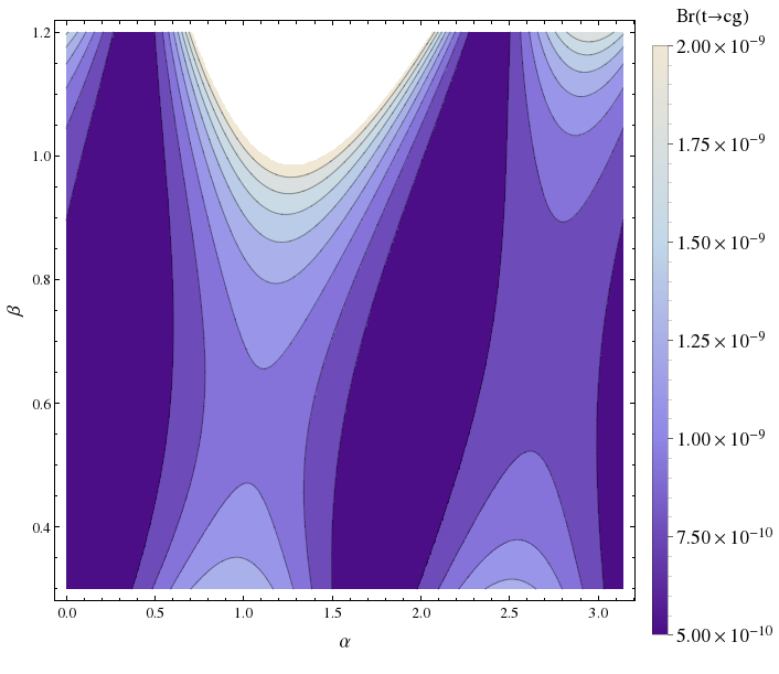
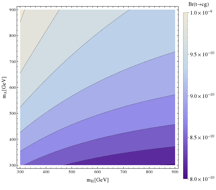
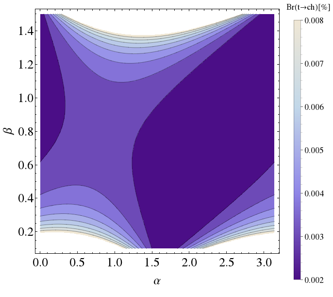
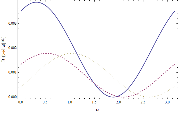
The tch𝑡𝑐t\rightarrow ch channel is particularly interesting since its branching ratio Br(thc)SM1015similar-to-or-equalsBrsubscript𝑡𝑐SMsuperscript1015\text{Br}(t\rightarrow hc)_{\text{SM}}\simeq 10^{-15} Aad:2014dya is extremely suppressed in the SM, but can be potentially large in our model allowing it to be probed at future collider experiments. As shown in Fig. 1 our model predictions can reach branching ratios of 𝒪(0.01%)𝒪percent0.01\mathcal{O}(0.01\%) in some regions of the αβ𝛼𝛽\alpha-\beta plane, allowing to further constrain our model parameter space with experimental searches for rare top decays.
Refer to caption
Refer to caption
Figure 1: (a)Br(thc)[%]\text{Br}(t\rightarrow hc)\left[\%\right] in the αβ𝛼𝛽\alpha-\beta plane. (b)Br(thc)[%]\text{Br}(t\rightarrow hc)\left[\%\right] as a function of α𝛼\alpha for β=π/10𝛽𝜋10\beta=\pi/10 (blue, solid), β=π/6𝛽𝜋6\beta=\pi/6 (red, dashed) and β=π/3𝛽𝜋3\beta=\pi/3 (yellow, dotted). The flavor violating ycth,Hsuperscriptsubscript𝑦𝑐𝑡𝐻y_{ct}^{h,H} couplings are enhanced for small β𝛽\beta values leading to a potentially large Br(thc)Br𝑡𝑐\text{Br}(t\rightarrow hc) observable at future experiments.

Recently an analysis of up-type FCNCs in the 2HDM type III has been performed Kim:2015zla parametrizing the flavor violating ycthsubscriptsuperscript𝑦𝑐𝑡y^{h}_{ct} coupling as ycth=1vλct2mtmcsuperscriptsubscript𝑦𝑐𝑡1𝑣subscript𝜆𝑐𝑡2subscript𝑚𝑡subscript𝑚𝑐y_{ct}^{h}=\frac{1}{v}\lambda_{ct}\sqrt{2m_{t}m_{c}} according to the Cheng–Sher Ansatz Cheng:1987rs (this type of FCNC was shown to be remarkably stable under radiative corrections Cvetic:1998uw ). Focusing on the cctt𝑐𝑐𝑡𝑡cc\rightarrow tt as well as the tcg𝑡𝑐𝑔t\rightarrow cg channels, they find that λctsubscript𝜆𝑐𝑡\lambda_{ct} can still take values of up to 1020102010-20 depending on the neutral heavy Higgs mass. With ycth1vVcbVtb2mtproportional-tosubscriptsuperscript𝑦𝑐𝑡1𝑣subscript𝑉𝑐𝑏subscript𝑉𝑡𝑏2subscript𝑚𝑡y^{h}_{ct}\propto\frac{1}{v}V_{cb}V_{tb}\sqrt{2}m_{t} our model corresponds to λct12subscript𝜆𝑐𝑡12\lambda_{ct}\approx\frac{1}{2} and is therefore well below the critical region. Indeed, following the analysis of Atwood:1996vj we find numerically that the loop induced decays tcg𝑡𝑐𝑔t\rightarrow cg, tcγ𝑡𝑐𝛾t\rightarrow c\gamma and tcZ𝑡𝑐𝑍t\rightarrow cZ are several orders of magnitude below the current LHC sensitivity. Explicitly, varying the free model parameters α,β𝛼𝛽\alpha,\beta and the scalar masses mH,mAsubscript𝑚𝐻subscript𝑚𝐴m_{H},m_{A} and mH±subscript𝑚superscript𝐻plus-or-minusm_{H^{\pm}}, we expect the branching ratios to be approximately

Br(tcg)𝒪(109),Br(tcγ)𝒪(1012),Br(tcZ)𝒪(1013),formulae-sequencesimilar-toBr𝑡𝑐𝑔𝒪superscript109formulae-sequencesimilar-toBr𝑡𝑐𝛾𝒪superscript1012similar-toBr𝑡𝑐𝑍𝒪superscript1013\displaystyle\text{Br}(t\rightarrow cg)\sim\mathcal{O}(10^{-9}),\qquad\text{Br}(t\rightarrow c\gamma)\sim\mathcal{O}(10^{-12}),\qquad\text{Br}(t\rightarrow cZ)\sim\mathcal{O}(10^{-13}), (163)

as opposed to the current upper limits from ATLAS and CMS Chatrchyan:2013nwa ; Aad:2015uza

Br(tcg)<1.6×10⁴,Br(tcγ,cZ)<5×10⁴.formulae-sequenceBr𝑡𝑐𝑔1.6superscript104Br𝑡𝑐𝛾𝑐𝑍5superscript104\displaystyle\text{Br}(t\rightarrow cg)<1.6\times 10^{-4},\qquad\text{Br}(t\rightarrow c\gamma,cZ)<5\times 10^{-4}. (164)

The largest branching ratio of the three channels, Br(tcg)Br𝑡𝑐𝑔\text{Br}(t\rightarrow cg), is shown in Fig. 2 as a function of α𝛼\alpha and β𝛽\beta for fixed mHsubscript𝑚𝐻m_{H} and mAsubscript𝑚𝐴m_{A} (a), as well as for variable mHsubscript𝑚𝐻m_{H} and mAsubscript𝑚𝐴m_{A} with fixed α𝛼\alpha and β𝛽\beta (b). As it turns out, the charged Higgs contribution is tiny and does not affect the prediction for any values of mH±subscript𝑚superscript𝐻plus-or-minusm_{H^{\pm}}.

Refer to caption
Refer to caption
Figure 2: (a)Br(thg)Br𝑡𝑔\text{Br}(t\rightarrow hg) in the αβ𝛼𝛽\alpha-\beta plane with mH=mA=500subscript𝑚𝐻subscript𝑚𝐴500m_{H}=m_{A}=500\,GeV. (b)Br(thg)Br𝑡𝑔\text{Br}(t\rightarrow hg) as a function of mHsubscript𝑚𝐻m_{H} and mAsubscript𝑚𝐴m_{A} for α=π/3𝛼𝜋3\alpha=\pi/3 and β=π/4𝛽𝜋4\beta=\pi/4. The decay rate is to a large extent independent of the charged Higgs mass mH±subscript𝑚superscript𝐻plus-or-minusm_{H^{\pm}}.

In the charged lepton sector we obtain

Yhlsuperscriptsubscript𝑌𝑙\displaystyle Y_{h}^{l} =2(yeehyeμhyeτhyμehyμμhyμτhyτehyτμhyττh)=2(cαmevsβ000mμsαvcβ000mτsαvcβ),absent2subscriptsuperscript𝑦𝑒𝑒subscriptsuperscript𝑦𝑒𝜇subscriptsuperscript𝑦𝑒𝜏subscriptsuperscript𝑦𝜇𝑒subscriptsuperscript𝑦𝜇𝜇subscriptsuperscript𝑦𝜇𝜏subscriptsuperscript𝑦𝜏𝑒subscriptsuperscript𝑦𝜏𝜇subscriptsuperscript𝑦𝜏𝜏2subscript𝑐𝛼subscript𝑚𝑒𝑣subscript𝑠𝛽000subscript𝑚𝜇subscript𝑠𝛼𝑣subscript𝑐𝛽000subscript𝑚𝜏subscript𝑠𝛼𝑣subscript𝑐𝛽\displaystyle=\sqrt{2}\left(\begin{array}[]{ccc}y^{h}_{ee}&y^{h}_{e\mu}&y^{h}_{e\tau}\\ y^{h}_{\mu e}&y^{h}_{\mu\mu}&y^{h}_{\mu\tau}\\ y^{h}_{\tau e}&y^{h}_{\tau\mu}&y^{h}_{\tau\tau}\end{array}\right)=\sqrt{2}\left(\begin{array}[]{ccc}-\frac{c_{\alpha}m_{e}}{vs_{\beta}}&0&0\\ 0&\frac{m_{\mu}s_{\alpha}}{vc_{\beta}}&0\\ 0&0&\frac{m_{\tau}s_{\alpha}}{vc_{\beta}}\end{array}\right), (171)
YHlsuperscriptsubscript𝑌𝐻𝑙\displaystyle Y_{H}^{l} =2(yeeHyeμHyeτHyμeHyμμHyμτHyτeHyτμHyττH)=2(mesαvsβ000cαmμvcβ000cαmτvcβ).absent2subscriptsuperscript𝑦𝐻𝑒𝑒subscriptsuperscript𝑦𝐻𝑒𝜇subscriptsuperscript𝑦𝐻𝑒𝜏subscriptsuperscript𝑦𝐻𝜇𝑒subscriptsuperscript𝑦𝐻𝜇𝜇subscriptsuperscript𝑦𝐻𝜇𝜏subscriptsuperscript𝑦𝐻𝜏𝑒subscriptsuperscript𝑦𝐻𝜏𝜇subscriptsuperscript𝑦𝐻𝜏𝜏2subscript𝑚𝑒subscript𝑠𝛼𝑣subscript𝑠𝛽000subscript𝑐𝛼subscript𝑚𝜇𝑣subscript𝑐𝛽000subscript𝑐𝛼subscript𝑚𝜏𝑣subscript𝑐𝛽\displaystyle=\sqrt{2}\left(\begin{array}[]{ccc}y^{H}_{ee}&y^{H}_{e\mu}&y^{H}_{e\tau}\\ y^{H}_{\mu e}&y^{H}_{\mu\mu}&y^{H}_{\mu\tau}\\ y^{H}_{\tau e}&y^{H}_{\tau\mu}&y^{H}_{\tau\tau}\end{array}\right)=\sqrt{2}\left(\begin{array}[]{ccc}-\frac{m_{e}s_{\alpha}}{vs_{\beta}}&0&0\\ 0&-\frac{c_{\alpha}m_{\mu}}{vc_{\beta}}&0\\ 0&0&-\frac{c_{\alpha}m_{\tau}}{vc_{\beta}}\end{array}\right). (178)

The charged leptons are also free of FCNCs due to the lack of off-diagonal Yukawa couplings. Consequently, the recently reported anomaly in hμτ𝜇𝜏h\rightarrow\mu\tau decays cannot be explained in our present model, even though it was possible to account for this in other multi-Higgs models with S3subscript𝑆3S_{3} or other discrete symmetries Campos:2014zaa ; Sierra:2014nqa ; Heeck:2014qea ; Varzielas:2015joa .

The charged Higgs couplings that are relevant, e.g., for Bs,d0B0¯s,dsubscriptsuperscript𝐵0𝑠𝑑subscript¯superscript𝐵0𝑠𝑑B^{0}_{s,d}-\overline{B^{0}}_{s,d} mixing and the radiative decays bqγ(q=s,d)𝑏𝑞𝛾𝑞𝑠𝑑b\rightarrow q\gamma\leavevmode\nobreak\ (q=s,d), are given by

YH±Lsuperscriptsubscript𝑌superscript𝐻plus-or-minus𝐿\displaystyle Y_{H^{\pm}}^{L} =2(yduydcydtysuyscystybuybcybt)=2(VudVtb2+Vcb2tβmuvVusVtbtβmcvVtdmtvtβVusVtb2+Vcb2tβmuvVudVtbtβmcvVtsmtvtβ00Vtbtβmtv),absent2subscript𝑦𝑑𝑢subscript𝑦𝑑𝑐subscript𝑦𝑑𝑡subscript𝑦𝑠𝑢subscript𝑦𝑠𝑐subscript𝑦𝑠𝑡subscript𝑦𝑏𝑢subscript𝑦𝑏𝑐subscript𝑦𝑏𝑡2subscript𝑉𝑢𝑑superscriptsubscript𝑉𝑡𝑏2superscriptsubscript𝑉𝑐𝑏2subscript𝑡𝛽subscript𝑚𝑢𝑣subscript𝑉𝑢𝑠subscript𝑉𝑡𝑏subscript𝑡𝛽subscript𝑚𝑐𝑣superscriptsubscript𝑉𝑡𝑑subscript𝑚𝑡𝑣subscript𝑡𝛽subscript𝑉𝑢𝑠superscriptsubscript𝑉𝑡𝑏2superscriptsubscript𝑉𝑐𝑏2subscript𝑡𝛽subscript𝑚𝑢𝑣subscript𝑉𝑢𝑑subscript𝑉𝑡𝑏subscript𝑡𝛽subscript𝑚𝑐𝑣superscriptsubscript𝑉𝑡𝑠subscript𝑚𝑡𝑣subscript𝑡𝛽00subscript𝑉𝑡𝑏subscript𝑡𝛽subscript𝑚𝑡𝑣\displaystyle=\sqrt{2}\left(\begin{array}[]{ccc}y_{du}&y_{dc}&y_{dt}\\ y_{su}&y_{sc}&y_{st}\\ y_{bu}&y_{bc}&y_{bt}\end{array}\right)=\sqrt{2}\left(\begin{array}[]{ccc}\frac{V_{ud}}{V_{tb}^{2}+V_{cb}^{2}}t_{\beta}\frac{m_{u}}{v}&-\frac{V_{us}}{V_{tb}}t_{\beta}\frac{m_{c}}{v}&-V_{td}^{\ast}\frac{m_{t}}{vt_{\beta}}\\ \frac{V_{us}}{V_{tb}^{2}+V_{cb}^{2}}t_{\beta}\frac{m_{u}}{v}&\frac{V_{ud}}{V_{tb}}t_{\beta}\frac{m_{c}}{v}&-V_{ts}^{\ast}\frac{m_{t}}{vt_{\beta}}\\ 0&0&V_{tb}t_{\beta}\frac{m_{t}}{v}\end{array}\right), (185)
YH±Rsuperscriptsubscript𝑌superscript𝐻plus-or-minus𝑅\displaystyle Y_{H^{\pm}}^{R} =2(yudyusyubycdycsycbytdytsytb)=2(VudmdvtβVusmsvtβVubtβmbvVcdmdvtβVcsmsvtβVcbtβmbvVtdmdvtβVtsmsvtβVtbtβmbv),absent2subscript𝑦𝑢𝑑subscript𝑦𝑢𝑠subscript𝑦𝑢𝑏subscript𝑦𝑐𝑑subscript𝑦𝑐𝑠subscript𝑦𝑐𝑏subscript𝑦𝑡𝑑subscript𝑦𝑡𝑠subscript𝑦𝑡𝑏2subscript𝑉𝑢𝑑subscript𝑚𝑑𝑣subscript𝑡𝛽subscript𝑉𝑢𝑠subscript𝑚𝑠𝑣subscript𝑡𝛽subscript𝑉𝑢𝑏subscript𝑡𝛽subscript𝑚𝑏𝑣subscript𝑉𝑐𝑑subscript𝑚𝑑𝑣subscript𝑡𝛽subscript𝑉𝑐𝑠subscript𝑚𝑠𝑣subscript𝑡𝛽subscript𝑉𝑐𝑏subscript𝑡𝛽subscript𝑚𝑏𝑣subscript𝑉𝑡𝑑subscript𝑚𝑑𝑣subscript𝑡𝛽subscript𝑉𝑡𝑠subscript𝑚𝑠𝑣subscript𝑡𝛽subscript𝑉𝑡𝑏subscript𝑡𝛽subscript𝑚𝑏𝑣\displaystyle=\sqrt{2}\left(\begin{array}[]{ccc}y_{ud}&y_{us}&y_{ub}\\ y_{cd}&y_{cs}&y_{cb}\\ y_{td}&y_{ts}&y_{tb}\end{array}\right)=\sqrt{2}\left(\begin{array}[]{ccc}V_{ud}\frac{m_{d}}{vt_{\beta}}&V_{us}\frac{m_{s}}{vt_{\beta}}&V_{ub}t_{\beta}\frac{m_{b}}{v}\\ V_{cd}\frac{m_{d}}{vt_{\beta}}&V_{cs}\frac{m_{s}}{vt_{\beta}}&V_{cb}t_{\beta}\frac{m_{b}}{v}\\ V_{td}\frac{m_{d}}{vt_{\beta}}&V_{ts}\frac{m_{s}}{vt_{\beta}}&V_{tb}t_{\beta}\frac{m_{b}}{v}\end{array}\right), (192)
YH±eνsuperscriptsubscript𝑌superscript𝐻plus-or-minus𝑒𝜈\displaystyle Y_{H^{\pm}}^{e\nu} =2mevtβ,YH±μν=2mμvtβ(cθlsθl),YH±τν=2mτvtβ(cθl+sθl),formulae-sequenceabsent2subscript𝑚𝑒𝑣subscript𝑡𝛽formulae-sequencesuperscriptsubscript𝑌superscript𝐻plus-or-minus𝜇𝜈2subscript𝑚𝜇𝑣subscript𝑡𝛽subscript𝑐subscript𝜃𝑙subscript𝑠subscript𝜃𝑙superscriptsubscript𝑌superscript𝐻plus-or-minus𝜏𝜈2subscript𝑚𝜏𝑣subscript𝑡𝛽subscript𝑐subscript𝜃𝑙subscript𝑠subscript𝜃𝑙\displaystyle=\sqrt{2}\frac{m_{e}}{vt_{\beta}},\qquad Y_{H^{\pm}}^{\mu\nu}=\sqrt{2}\frac{m_{\mu}}{v}t_{\beta}\left(c_{\theta_{l}}-s_{\theta_{l}}\right),\qquad Y_{H^{\pm}}^{\tau\nu}=\sqrt{2}\frac{m_{\tau}}{v}t_{\beta}\left(c_{\theta_{l}}+s_{\theta_{l}}\right), (193)

where in the last equation we summed over the neutrino mass eigenstates as they are usually undetected in typical flavor experiments. Here, the couplings ybusubscript𝑦𝑏𝑢y_{bu} and ybcsubscript𝑦𝑏𝑐y_{bc} that could be used to explain the outstanding anomaly in BD()τν𝐵superscript𝐷𝜏𝜈B\rightarrow D^{(\ast)}\tau\nu decays Lees:2013uzd are zero, hence no difference from 2HDMs of type II is to be expected in these channels.

On the other hand, the charged scalar sector is tightly constrained by bsγ𝑏𝑠𝛾b\rightarrow s\gamma measurements, where the charged scalar H±superscript𝐻plus-or-minusH^{\pm} leads to an additional loop diagram replacing the W±superscript𝑊plus-or-minusW^{\pm}. Recently a lower bound of 480GeV480GeV480\,\text{GeV} was placed on the charged Higgs in the 2HDM type II Misiak:2015xwa . Following the analysis of Trott:2010iz we estimate a lower bound on the charged Higgs mass imposed on our model by constraints on the Wilson coefficients involved in Br(bsγ)Br𝑏𝑠𝛾\text{Br}(b\rightarrow s\gamma). Since tanβ𝛽\tan\beta drops out in the product of the corresponding Yukawa couplings ytb(ybt)subscript𝑦𝑡𝑏subscript𝑦𝑏𝑡y_{tb}(y_{bt}) and yts(yst)subscript𝑦𝑡𝑠subscript𝑦𝑠𝑡y_{ts}(y_{st}), the prediction is independent of tanβ𝛽\tan\beta and the lower limit is roughly mH±500GeVgreater-than-or-equivalent-tosubscript𝑚superscript𝐻plus-or-minus500GeVm_{H^{\pm}}\gtrsim 500\,\text{GeV}.

III.1 Constraints from hγγ𝛾𝛾h\rightarrow\gamma\gamma

In our 2HDM the hγγ𝛾𝛾h\rightarrow\gamma\gamma decay receives additional contributions from loops with charged scalars H±superscript𝐻plus-or-minusH^{\pm}, as shown in Fig. 3, and therefore sets bounds on the masses of these scalars as well as on the angles α𝛼\alpha and β𝛽\beta.

Refer to caption
Figure 3: One-loop Feynman diagrams in the Unitary Gauge contributing to the hγγ𝛾𝛾h\rightarrow\gamma\gamma decay.

The explicit form of the hγγ𝛾𝛾h\rightarrow\gamma\gamma decay rate is Shifman:1979eb ; Gavela:1981ri ; Kalyniak:1985ct ; Gunion:1989we ; Spira:1997dg ; Djouadi:2005gj ; Marciano:2011gm ; Wang:2012gm

Γ(hγγ)=αem2mh3256π3v2|fahffNcQf2F1/2(ϱf)+ahWWF1(ϱW)+λhH±Hv2mH±2F0(ϱH±)|2.Γ𝛾𝛾superscriptsubscript𝛼𝑒𝑚2superscriptsubscript𝑚3256superscript𝜋3superscript𝑣2superscriptsubscript𝑓subscript𝑎𝑓𝑓subscript𝑁𝑐superscriptsubscript𝑄𝑓2subscript𝐹12subscriptitalic-ϱ𝑓subscript𝑎𝑊𝑊subscript𝐹1subscriptitalic-ϱ𝑊subscript𝜆superscript𝐻plus-or-minussuperscript𝐻minus-or-plus𝑣2superscriptsubscript𝑚superscript𝐻plus-or-minus2subscript𝐹0subscriptitalic-ϱsuperscript𝐻plus-or-minus2\Gamma\left(h\rightarrow\gamma\gamma\right)=\frac{\alpha_{em}^{2}m_{h}^{3}}{256\pi^{3}v^{2}}\left|\sum_{f}a_{hff}N_{c}Q_{f}^{2}F_{1/2}\left(\varrho_{f}\right)+a_{hWW}F_{1}\left(\varrho_{W}\right)+\frac{\lambda_{hH^{\pm}H^{\mp}}v}{2m_{H^{\pm}}^{2}}F_{0}\left(\varrho_{H^{\pm}}\right)\right|^{2}\,. (194)

Here ϱisubscriptitalic-ϱ𝑖\varrho_{i} are the mass ratios ϱi=mh24Mi2subscriptitalic-ϱ𝑖superscriptsubscript𝑚24superscriptsubscript𝑀𝑖2\varrho_{i}=\frac{m_{h}^{2}}{4M_{i}^{2}}, with Mi=mf,MWsubscript𝑀𝑖subscript𝑚𝑓subscript𝑀𝑊M_{i}=m_{f},M_{W}, and mH±subscript𝑚superscript𝐻plus-or-minusm_{H^{\pm}}, αemsubscript𝛼𝑒𝑚\alpha_{em} is the fine structure constant, NCsubscript𝑁𝐶N_{C} is the color factor (NC=1subscript𝑁𝐶1N_{C}=1 for leptons, NC=3subscript𝑁𝐶3N_{C}=3 for quarks), and Qfsubscript𝑄𝑓Q_{f} is the electric charge of the fermion in the loop. From the fermion-loop contributions we consider only the dominant top quark term. Furthermore, λhH±Hsubscript𝜆superscript𝐻plus-or-minussuperscript𝐻minus-or-plus\lambda_{hH^{\pm}H^{\mp}} is the trilinear coupling between the SM-like Higgs and a pair of charged Higgses, which is given by

λhH±H=γ12+κ122vsin2βcos(α+β).subscript𝜆superscript𝐻plus-or-minussuperscript𝐻minus-or-plussubscript𝛾12subscript𝜅122𝑣2𝛽𝛼𝛽\lambda_{hH^{\pm}H^{\mp}}=-\frac{\gamma_{12}+\kappa_{12}}{2}v\sin 2\beta\cos\left(\alpha+\beta\right). (195)

Besides that ahttsubscript𝑎𝑡𝑡a_{htt} and ahWWsubscript𝑎𝑊𝑊a_{hWW} are the deviation factors from the SM Higgs-top quark coupling and the SM Higgs- W𝑊W gauge boson coupling, respectively (in the SM these factors are unity). These deviation factors are given by

ahttsubscript𝑎𝑡𝑡\displaystyle a_{htt} similar-to-or-equals\displaystyle\simeq sinαcosβ,𝛼𝛽\displaystyle\frac{\sin\alpha}{\cos\beta}, (196)
ahWWsubscript𝑎𝑊𝑊\displaystyle a_{hWW} =\displaystyle= sin(αβ),𝛼𝛽\displaystyle\sin\left(\alpha-\beta\right), (197)

where in ahttsubscript𝑎𝑡𝑡a_{htt} we neglected the contribution suppressed by small CKM entries.

The dimensionless loop factors F1/2(ϱ)subscript𝐹12italic-ϱF_{1/2}\left(\varrho\right) and F1(ϱ)subscript𝐹1italic-ϱF_{1}\left(\varrho\right) (for spin-1/2121/2 and spin-111 particles in the loop, respectively) are Gunion:1989we ; Djouadi:2005gj

F1/2(ϱ)subscript𝐹12italic-ϱ\displaystyle F_{1/2}\left(\varrho\right) =2[ϱ+(ϱ1)f(ϱ)]ϱ2,absent2delimited-[]italic-ϱitalic-ϱ1𝑓italic-ϱsuperscriptitalic-ϱ2\displaystyle=2\left[\varrho+\left(\varrho-1\right)f\left(\varrho\right)\right]\varrho^{-2}, (198)
F1(ϱ)subscript𝐹1italic-ϱ\displaystyle F_{1}\left(\varrho\right) =[2ϱ2+3ϱ+3(2ϱ1)f(ϱ)]ϱ2,absentdelimited-[]2superscriptitalic-ϱ23italic-ϱ32italic-ϱ1𝑓italic-ϱsuperscriptitalic-ϱ2\displaystyle=-\left[2\varrho^{2}+3\varrho+3\left(2\varrho-1\right)f\left(\varrho\right)\right]\varrho^{-2}, (199)
F0(ϱ)subscript𝐹0italic-ϱ\displaystyle F_{0}\left(\varrho\right) =[ϱf(ϱ)]ϱ2,absentdelimited-[]italic-ϱ𝑓italic-ϱsuperscriptitalic-ϱ2\displaystyle=-\left[\varrho-f\left(\varrho\right)\right]\varrho^{-2}, (200)

with

f(ϱ)={arcsin2ϱ,𝑓𝑜𝑟ϱ114[ln(1+1ϱ111ϱ1)iπ]2,𝑓𝑜𝑟ϱ>1.𝑓italic-ϱcasessuperscript2italic-ϱ𝑓𝑜𝑟italic-ϱ1otherwise14superscriptdelimited-[]11superscriptitalic-ϱ111superscriptitalic-ϱ1𝑖𝜋2𝑓𝑜𝑟italic-ϱ1otherwisef\left(\varrho\right)=\begin{cases}\arcsin^{2}\sqrt{\varrho},\hskip 14.22636pt\mathit{for}\hskip 5.69046pt\varrho\leq 1\\ -\frac{1}{4}\left[\ln\left(\frac{1+\sqrt{1-\varrho^{-1}}}{1-\sqrt{1-\varrho^{-1}}}\right)-i\pi\right]^{2},\hskip 14.22636pt\mathit{for}\hskip 5.69046pt\varrho>1.\end{cases} (201)

In what follows we determine the constraints that the Higgs diphoton signal strength imposes on our model. To this end, we introduce the ratio Rγγsubscript𝑅𝛾𝛾R_{\gamma\gamma}, which normalizes the γγ𝛾𝛾\gamma\gamma signal predicted by our model relative to that of the SM:

Rγγ=σ(pph)Γ(hγγ)σ(pph)SMΓ(hγγ)SMahtt2Γ(hγγ)Γ(hγγ)SM.subscript𝑅𝛾𝛾𝜎𝑝𝑝Γ𝛾𝛾𝜎subscript𝑝𝑝𝑆𝑀Γsubscript𝛾𝛾𝑆𝑀similar-to-or-equalssuperscriptsubscript𝑎𝑡𝑡2Γ𝛾𝛾Γsubscript𝛾𝛾𝑆𝑀R_{\gamma\gamma}=\frac{\sigma\left(pp\rightarrow h\right)\Gamma\left(h\rightarrow\gamma\gamma\right)}{\sigma\left(pp\rightarrow h\right)_{SM}\Gamma\left(h\rightarrow\gamma\gamma\right)_{SM}}\simeq a_{htt}^{2}\frac{\Gamma\left(h\rightarrow\gamma\gamma\right)}{\Gamma\left(h\rightarrow\gamma\gamma\right)_{SM}}. (202)

The normalization given by Eq. (202) for hγγ𝛾𝛾h\rightarrow\gamma\gamma was also used in Refs. Wang:2012gm ; Carcamo-Hernandez:2013ypa ; Bhattacharyya:2014oka ; Fortes:2014dia ; Campos:2014zaa ; Hernandez:2015xka ; Hernandez:2015nga .

The ratio Rγγsubscript𝑅𝛾𝛾R_{\gamma\gamma} has been measured by CMS and ATLAS with the best-fit signals Khachatryan:2014ira ; Aad:2014eha

RγγCMS=1.140.23+0.26andRγγATLAS=1.17±0.27.formulae-sequencesuperscriptsubscript𝑅𝛾𝛾CMSsuperscriptsubscript1.140.230.26andsuperscriptsubscript𝑅𝛾𝛾ATLASplus-or-minus1.170.27R_{\gamma\gamma}^{\text{CMS}}=1.14_{-0.23}^{+0.26}\qquad\text{and}\qquad R_{\gamma\gamma}^{\text{ATLAS}}=1.17\pm 0.27.

Figure (4(a)) shows the sensitivity of the ratio Rγγsubscript𝑅𝛾𝛾R_{\gamma\gamma} under variations of the mixing angle α𝛼\alpha for mH±=500subscript𝑚superscript𝐻plus-or-minus500m_{H^{\pm}}=500 GeV, γ12+κ12=1subscript𝛾12subscript𝜅121\gamma_{12}+\kappa_{12}=1 and different values of the mixing angle β𝛽\beta. It follows that as the mixing angle β𝛽\beta is increased, the range of α𝛼\alpha consistent with LHC observations of hγγ𝛾𝛾h\rightarrow\gamma\gamma moves away from π/2𝜋2\pi/2. On the other hand, the decay rate is largely independent of the charged Higgs mass or the sum of the couplings γ12+κ12subscript𝛾12subscript𝜅12\gamma_{12}+\kappa_{12}, which is consistent with the contribution mediated by charged scalars to the hγγ𝛾𝛾h\rightarrow\gamma\gamma process being a small correction. In fact we checked numerically it stays almost constant when mH±subscript𝑚superscript𝐻plus-or-minusm_{H^{\pm}} is varied from 500500500 GeV to 111 TeV for fixed values of α,β𝛼𝛽\alpha,\beta, and the quartic couplings of the scalar potential. For the same values of the charged Higgs mass and quartic couplings, we show in Figure (4(b)) the Z-shaped allowed region in the α𝛼\alpha-β𝛽\beta plane that is consistent with the Higgs diphoton decay rate constraints at the LHC, and overlay it with the relatively weak bound in Eq. (162) that arises from top quark FCNCs.
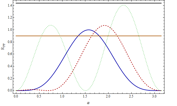
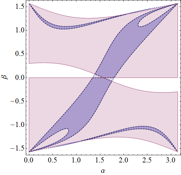
Refer to caption
Refer to caption
Figure 4: The constraints on the model imposed by keeping Rγγsubscript𝑅𝛾𝛾R_{\gamma\gamma} inside the experimentally allowed 1σ𝜎\sigma range determined by CMS and ATLAS to be 1.140.23+0.26subscriptsuperscript1.140.260.231.14^{+0.26}_{-0.23} and 1.17±0.27plus-or-minus1.170.271.17\pm 0.27, respectively Khachatryan:2014ira ; Aad:2014eha . (4.(a)) shows the ratio Rγγsubscript𝑅𝛾𝛾R_{\gamma\gamma} as a function of the mixing angle α𝛼\alpha of the CP-even neutral scalars hh and H0superscript𝐻0H^{0} for mH±=500subscript𝑚superscript𝐻plus-or-minus500m_{H^{\pm}}=500 GeV, γ12+κ12=1subscript𝛾12subscript𝜅121\gamma_{12}+\kappa_{12}=1 and different values of the mixing angle β𝛽\beta; the blue, red and green curves correspond β𝛽\beta set to 00, π6𝜋6\frac{\pi}{6} and π3𝜋3\frac{\pi}{3}, respectively, and the horizontal lines are the minimum and maximum values of the ratio Rγγsubscript𝑅𝛾𝛾R_{\gamma\gamma}. (4.(b)) shows the allowed region in the α𝛼\alpha-β𝛽\beta plane consistent with the Higgs diphoton decay rate constraint at the LHC, superimposed with the constraint imposed by Eq.(162).

III.2 T𝑇T and S𝑆S parameters

The extra scalars affect the oblique corrections of the SM, and these values are measured in high precision experiments. Consequently, they act as a further constraint on the validity of our model. The oblique corrections are parametrized in terms of the two well-known quantities T𝑇T and S𝑆S. In this section we calculate one-loop contributions to the oblique parameters T𝑇T and S𝑆S defined as Peskin:1991sw ; Altarelli:1990zd ; Barbieri:2004qk

T=Π33(q2)Π11(q2)αEM(MZ)MW2|q2=0,S=2sin2θWαEM(MZ)dΠ30(q2)dq2|q2=0.T=\frac{\Pi_{33}\left(q^{2}\right)-\Pi_{11}\left(q^{2}\right)}{\alpha_{EM}(M_{Z})M_{W}^{2}}\biggl{|}_{q^{2}=0},\ \ \ \ \ \ \ \ \ \ \ S=\frac{2\sin 2{\theta}_{W}}{\alpha_{EM}(M_{Z})}\frac{d\Pi_{30}\left(q^{2}\right)}{dq^{2}}\biggl{|}_{q^{2}=0}. (203)

Π11(0)subscriptΠ110\Pi_{11}\left(0\right), Π33(0)subscriptΠ330\Pi_{33}\left(0\right), and Π30(q2)subscriptΠ30superscript𝑞2\Pi_{30}\left(q^{2}\right) are the vacuum polarization amplitudes with {Wμ1,Wμ1}superscriptsubscript𝑊𝜇1superscriptsubscript𝑊𝜇1\{W_{\mu}^{1},W_{\mu}^{1}\}, {Wμ3,Wμ3}superscriptsubscript𝑊𝜇3superscriptsubscript𝑊𝜇3\{W_{\mu}^{3},W_{\mu}^{3}\} and {Wμ3,Bμ}superscriptsubscript𝑊𝜇3subscript𝐵𝜇\{W_{\mu}^{3},B_{\mu}\} external gauge bosons, respectively, where q𝑞q is their momentum. We note that in the definitions of the T𝑇T and S𝑆S parameters, the new physics is assumed to be heavy when compared to MWsubscript𝑀𝑊M_{W} and MZsubscript𝑀𝑍M_{Z}.

The Feynman diagrams contributing to the T𝑇T and S𝑆S parameters are shown in Figs. 5 and 6.

Refer to caption
Figure 5: One-loop Feynman diagrams contributing to the T𝑇T parameter. The fields H1superscript𝐻1H^{1} and H2superscript𝐻2H^{2} are linear combinations of the charged Higgses H±superscript𝐻plus-or-minusH^{\pm}, similarly to how W±superscript𝑊plus-or-minusW^{\pm} gauge bosons are defined in terms of W1superscript𝑊1W^{1} and W2superscript𝑊2W^{2}. Likewise, the fields π1superscript𝜋1\pi^{1} and π2superscript𝜋2\pi^{2} are linear combinations of the charged Goldstone bosons π±superscript𝜋plus-or-minus\pi^{\pm}.
Refer to caption
Figure 6: One-loop Feynman diagrams contributing to the S𝑆S parameter. The fields H1superscript𝐻1H^{1} and H2superscript𝐻2H^{2} are linear combinations of the charged Higgses H±superscript𝐻plus-or-minusH^{\pm}, similarly to how W±superscript𝑊plus-or-minusW^{\pm} gauge bosons are defined in terms of W1superscript𝑊1W^{1} and W2superscript𝑊2W^{2}.

We split the T𝑇T and S𝑆S emphasizing the contributions arising from new physics as T=TSM+ΔT𝑇subscript𝑇𝑆𝑀Δ𝑇T=T_{SM}+\Delta T and S=SSM+ΔS𝑆subscript𝑆𝑆𝑀Δ𝑆S=S_{SM}+\Delta S, where TSMsubscript𝑇𝑆𝑀T_{SM} and SSMsubscript𝑆𝑆𝑀S_{SM} are the SM contributions given by

TSM=316πcos2θWln(mh2mW2),subscript𝑇𝑆𝑀316𝜋superscript2subscript𝜃𝑊superscriptsubscript𝑚2superscriptsubscript𝑚𝑊2T_{SM}=-\frac{3}{16\pi\cos^{2}\theta_{W}}\ln\left(\frac{m_{h}^{2}}{m_{W}^{2}}\right), (204)
SSM=112πln(mh2mW2),subscript𝑆𝑆𝑀112𝜋superscriptsubscript𝑚2superscriptsubscript𝑚𝑊2S_{SM}=\frac{1}{12\pi}\ln\left(\frac{m_{h}^{2}}{m_{W}^{2}}\right), (205)

while ΔTΔ𝑇\Delta T and ΔSΔ𝑆\Delta S contain all the contributions involving in our model the heavy scalars

ΔTΔ𝑇\displaystyle\Delta T similar-to-or-equals\displaystyle\simeq 3cos2(αβ)16πcos2θWln(mH02mh2)+116π2v2αEM(MZ)[mH±2F(mA02,mH±2)]3superscript2𝛼𝛽16𝜋superscript2subscript𝜃𝑊superscriptsubscript𝑚superscript𝐻02superscriptsubscript𝑚2116superscript𝜋2superscript𝑣2subscript𝛼𝐸𝑀subscript𝑀𝑍delimited-[]superscriptsubscript𝑚superscript𝐻plus-or-minus2𝐹superscriptsubscript𝑚superscript𝐴02superscriptsubscript𝑚superscript𝐻plus-or-minus2\displaystyle-\frac{3\cos^{2}\left(\alpha-\beta\right)}{16\pi\cos^{2}\theta_{W}}\ln\left(\frac{m_{H^{0}}^{2}}{m_{h}^{2}}\right)+\frac{1}{16\pi^{2}v^{2}\alpha_{EM}(M_{Z})}\left[m_{H^{\pm}}^{2}-F\left(m_{A^{0}}^{2},m_{H^{\pm}}^{2}\right)\right] (206)
+sin2(αβ)16π2v2αEM(MZ)[F(mh2,mA02)F(mh2,mH±2)]superscript2𝛼𝛽16superscript𝜋2superscript𝑣2subscript𝛼𝐸𝑀subscript𝑀𝑍delimited-[]𝐹superscriptsubscript𝑚2superscriptsubscript𝑚superscript𝐴02𝐹superscriptsubscript𝑚2superscriptsubscript𝑚superscript𝐻plus-or-minus2\displaystyle+\frac{\sin^{2}\left(\alpha-\beta\right)}{16\pi^{2}v^{2}\alpha_{EM}(M_{Z})}\left[F\left(m_{h}^{2},m_{A^{0}}^{2}\right)-F\left(m_{h}^{2},m_{H^{\pm}}^{2}\right)\right]
+cos2(αβ)16π2v2αEM(MZ)[F(mH02,mA02)F(mH02,mH±2)],superscript2𝛼𝛽16superscript𝜋2superscript𝑣2subscript𝛼𝐸𝑀subscript𝑀𝑍delimited-[]𝐹superscriptsubscript𝑚superscript𝐻02superscriptsubscript𝑚superscript𝐴02𝐹superscriptsubscript𝑚superscript𝐻02superscriptsubscript𝑚superscript𝐻plus-or-minus2\displaystyle+\frac{\cos^{2}\left(\alpha-\beta\right)}{16\pi^{2}v^{2}\alpha_{EM}(M_{Z})}\left[F\left(m_{H^{0}}^{2},m_{A^{0}}^{2}\right)-F\left(m_{H^{0}}^{2},m_{H^{\pm}}^{2}\right)\right],
ΔS112π[cos2(αβ)ln(mH02mh2)+sin2(αβ)K(mh2,mA02,mH±2)+cos2(αβ)K(mH02,mA02,mH±2)],similar-to-or-equalsΔ𝑆112𝜋delimited-[]superscript2𝛼𝛽superscriptsubscript𝑚superscript𝐻02superscriptsubscript𝑚2superscript2𝛼𝛽𝐾superscriptsubscript𝑚2superscriptsubscript𝑚superscript𝐴02superscriptsubscript𝑚superscript𝐻plus-or-minus2superscript2𝛼𝛽𝐾superscriptsubscript𝑚superscript𝐻02superscriptsubscript𝑚superscript𝐴02superscriptsubscript𝑚superscript𝐻plus-or-minus2\Delta S\simeq\frac{1}{12\pi}\left[\cos^{2}\left(\alpha-\beta\right)\ln\left(\frac{m_{H^{0}}^{2}}{m_{h}^{2}}\right)+\sin^{2}\left(\alpha-\beta\right)K\left(m_{h}^{2},m_{A^{0}}^{2},m_{H^{\pm}}^{2}\right)+\cos^{2}\left(\alpha-\beta\right)K\left(m_{H^{0}}^{2},m_{A^{0}}^{2},m_{H^{\pm}}^{2}\right)\right], (207)

where we introduced the functions Bertolini:1985ia ; Hollik:1986gg ; Hollik:1987fg ; Gunion:1989we ; Froggatt:1991qw ; Grimus:2008nb ; Haber:2010bw ; Hernandez:2015rfa

F(m12,m22)=m12m22m12m22ln(m12m22),limm2m1F(m12,m22)=m12,formulae-sequence𝐹superscriptsubscript𝑚12superscriptsubscript𝑚22superscriptsubscript𝑚12superscriptsubscript𝑚22superscriptsubscript𝑚12superscriptsubscript𝑚22superscriptsubscript𝑚12superscriptsubscript𝑚22subscriptsubscript𝑚2subscript𝑚1𝐹superscriptsubscript𝑚12superscriptsubscript𝑚22superscriptsubscript𝑚12F\left(m_{1}^{2},m_{2}^{2}\right)=\frac{m_{1}^{2}m_{2}^{2}}{m_{1}^{2}-m_{2}^{2}}\ln\left(\frac{m_{1}^{2}}{m_{2}^{2}}\right),\hskip 42.67912pt\hskip 42.67912pt\lim_{m_{2}\rightarrow m_{1}}F\left(m_{1}^{2},m_{2}^{2}\right)=m_{1}^{2}, (208)
K(m12,m22,m32)𝐾superscriptsubscript𝑚12superscriptsubscript𝑚22superscriptsubscript𝑚32\displaystyle K\left(m_{1}^{2},m_{2}^{2},m_{3}^{2}\right) =\displaystyle= 1(m22m12)3{m14(3m22m12)ln(m12m32)m24(3m12m22)ln(m22m32)\displaystyle\frac{1}{\left(m_{2}^{2}-m_{1}^{2}\right){}^{3}}\left\{m_{1}^{4}\left(3m_{2}^{2}-m_{1}^{2}\right)\ln\left(\frac{m_{1}^{2}}{m_{3}^{2}}\right)-m_{2}^{4}\left(3m_{1}^{2}-m_{2}^{2}\right)\ln\left(\frac{m_{2}^{2}}{m_{3}^{2}}\right)\right. (209)
16[27m12m22(m12m22)+5(m26m16)]},\displaystyle-\left.\frac{1}{6}\left[27m_{1}^{2}m_{2}^{2}\left(m_{1}^{2}-m_{2}^{2}\right)+5\left(m_{2}^{6}-m_{1}^{6}\right)\right]\right\},

with the properties

limm1m2K(m12,m22,m32)subscriptsubscript𝑚1subscript𝑚2𝐾superscriptsubscript𝑚12superscriptsubscript𝑚22superscriptsubscript𝑚32\displaystyle\lim_{m_{1}\rightarrow m_{2}}K(m_{1}^{2},m_{2}^{2},m_{3}^{2}) =\displaystyle= K1(m22,m32)=ln(m22m32),subscript𝐾1superscriptsubscript𝑚22superscriptsubscript𝑚32superscriptsubscript𝑚22superscriptsubscript𝑚32\displaystyle K_{1}(m_{2}^{2},m_{3}^{2})=\ln\left(\frac{m_{2}^{2}}{m_{3}^{2}}\right),
limm2m3K(m12,m22,m32)subscriptsubscript𝑚2subscript𝑚3𝐾superscriptsubscript𝑚12superscriptsubscript𝑚22superscriptsubscript𝑚32\displaystyle\lim_{m_{2}\rightarrow m_{3}}K(m_{1}^{2},m_{2}^{2},m_{3}^{2}) =\displaystyle= K2(m12,m32)=5m16+27m14m3227m12m34+6(m163m14m32)ln(m12m32)+5m366(m12m32)3,subscript𝐾2superscriptsubscript𝑚12superscriptsubscript𝑚325superscriptsubscript𝑚1627superscriptsubscript𝑚14superscriptsubscript𝑚3227superscriptsubscript𝑚12superscriptsubscript𝑚346superscriptsubscript𝑚163superscriptsubscript𝑚14superscriptsubscript𝑚32superscriptsubscript𝑚12superscriptsubscript𝑚325superscriptsubscript𝑚366superscriptsuperscriptsubscript𝑚12superscriptsubscript𝑚323\displaystyle K_{2}(m_{1}^{2},m_{3}^{2})=\frac{-5m_{1}^{6}+27m_{1}^{4}m_{3}^{2}-27m_{1}^{2}m_{3}^{4}+6\left(m_{1}^{6}-3m_{1}^{4}m_{3}^{2}\right)\ln\left(\frac{m_{1}^{2}}{m_{3}^{2}}\right)+5m_{3}^{6}}{6\left(m_{1}^{2}-m_{3}^{2}\right)^{3}},
limm1m3K(m12,m22,m32)subscriptsubscript𝑚1subscript𝑚3𝐾superscriptsubscript𝑚12superscriptsubscript𝑚22superscriptsubscript𝑚32\displaystyle\lim_{m_{1}\rightarrow m_{3}}K(m_{1}^{2},m_{2}^{2},m_{3}^{2}) =\displaystyle= K2(m22,m32).subscript𝐾2superscriptsubscript𝑚22superscriptsubscript𝑚32\displaystyle K_{2}(m_{2}^{2},m_{3}^{2}). (210)

The experimental results on T𝑇T and S𝑆S restrict ΔTΔ𝑇\Delta T and ΔSΔ𝑆\Delta S to lie inside a region in the ΔSΔTΔ𝑆Δ𝑇\Delta S-\Delta T plane. At the 95%percent9595\% confidence level, these are the elliptic contours shown in Fig. 7. The origin ΔS=ΔT=0Δ𝑆Δ𝑇0\Delta S=\Delta T=0 is the SM value with mh=125.5subscript𝑚125.5m_{h}=125.5 GeV and mt=176subscript𝑚𝑡176m_{t}=176 GeV. We analyze the T𝑇T and S𝑆S parameter constraints on our model by considering two benchmark scenarios, in both keeping αβ=π5𝛼𝛽𝜋5\alpha-\beta=\frac{\pi}{5}. In the first scenario we assume that the CP-even and CP-odd neutral Higgs bosons have degenerate masses of 500500500 GeV, below which the LHC has not detected any scalars beyond the SM-like state. In this first scenario, we find that the T𝑇T and S𝑆S parameters constrain the charged Higgs masses to the range 550550550 GeV mH±absentsubscript𝑚superscript𝐻plus-or-minusabsent\leq m_{H^{\pm}}\leq 580580580 GeV, which is consistent with the lower bound mH±500greater-than-or-equivalent-tosubscript𝑚superscript𝐻plus-or-minus500m_{H^{\pm}}\gtrsim 500 GeV obtained from bsγ𝑏𝑠𝛾b\to s\gamma constraints Misiak:2015xwa . In the second scenario, we assume that the charged Higgses and CP-even neutral Higgses have degenerate masses of 500500500 GeV. In this second scenario, the T𝑇T and S𝑆S parameter constraints are fulfilled if the CP-odd neutral Higgs boson mass is in the range 375375375 GeV mA0absentsubscript𝑚superscript𝐴0absent\leq m_{A^{0}}\leq 495495495 GeV.

Refer to caption
Refer to caption

7.a)                                               (7.b)

Figure 7: The ΔSΔTΔ𝑆Δ𝑇\Delta S-\Delta T plane, where the ellipses contain the experimentally allowed region at 95%percent9595\% confidence level taken from Baak:2013ppa ; Baak:2012kk ; Baak:2011ze . We set αβ=π5𝛼𝛽𝜋5\alpha-\beta=\frac{\pi}{5}. Figures (a) and (b) correspond to mA0=mH0=500subscript𝑚superscript𝐴0subscript𝑚superscript𝐻0500m_{A^{0}}=m_{{H}^{0}}=500 GeV and mH0=mH±=500subscript𝑚superscript𝐻0subscript𝑚superscript𝐻plus-or-minus500m_{H^{0}}=m_{H^{\pm}}=500 GeV, respectively. The charged Higgs and CP-odd neutral Higgs boson masses vary between 550550550 GeV mH±absentsubscript𝑚superscript𝐻plus-or-minusabsent\leq m_{H^{\pm}}\leq 580580580 GeV (Fig. 7(a), 375375375 GeV mA0absentsubscript𝑚superscript𝐴0absent\leq m_{A^{0}}\leq 495495495 GeV (Fig. 7(b). The nearly vertical lines going up towards the ellipses correspond to ΔTΔ𝑇\Delta T and ΔSΔ𝑆\Delta S parameters in our model as masses are varied in the aforementioned ranges.

IV Conclusions

We have constructed a viable 2-Higgs doublet extension of the Standard Model which features additionally an S3subscript𝑆3S_{3} flavor symmetry and extra scalars that break S3subscript𝑆3S_{3}. This leads to textures for fermion masses, and consists in an existence proof of models leading to the quark texture in Hernandez:2014zsa . Overall, the model can fit the observed masses, CKM and PMNS mixing angles very well. The model has in total seventeen effective free parameters, which are fitted to reproduce the experimental values of eighteen observables in the quark and lepton sectors, i.e., nine charged fermion masses, two neutrino mass squared splittings, three lepton mixing parameters, three quark mixing angles and one CP violating phase of the CKM quark mixing matrix. The model predicts one massless neutrino for both normal and inverted hierarchies in the active neutrino mass spectrum as well as an effective Majorana neutrino mass, relevant for neutrinoless double beta decay, with values mββ=subscript𝑚𝛽𝛽absentm_{\beta\beta}= 4 meV and 50 meV, for the normal and the inverted neutrino spectrum, respectively. In the latter case our prediction is within the declared reach of the next generation bolometric CUORE experiment Alessandria:2011rc or, more realistically, of the next-to-next generation tonne-scale 0νββ0𝜈𝛽𝛽0\nu\beta\beta-decay experiments. The sum of the light active neutrino masses in our model is 595959 meV and 0.10.10.1 eV for the normal and the inverted neutrino spectrum, respectively, which is consistent with the cosmological bound k=13mνk<0.23subscriptsuperscript3𝑘1subscript𝑚subscript𝜈𝑘0.23\sum^{3}_{k=1}m_{\nu_{k}}<0.23 eV. The additional scalars mediate flavor changing neutral current processes, but due to the specific shape of the Yukawa couplings dictated by the flavor symmetry these processes occur only in the up-type quark sector. In the scalar sector the enlarged field content of the model leads to constraints from both rare top decays and from a hγγ𝛾𝛾h\to\gamma\gamma rate that can be distinguished from the SM prediction. Among rare top decays, tch𝑡𝑐t\to ch is particularly promising as its branching ratio can reach 𝒪(0.01%)𝒪percent0.01\mathcal{O}(0.01\%) in our model. With respect to the hγγ𝛾𝛾h\to\gamma\gamma, we find that it depends only slightly on the mass of the charged Higgs and the dependence on the quartic scalar couplings is negligible, but the dominant top quark and vector boson contributions are modified in our model and allow us to place constraints on the hierarchy of the SU(2)𝑆𝑈2SU(2) doublet VEVs (β𝛽\beta) and the mixing of their CP-even mass eigenstates (α𝛼\alpha) that are much stronger than those obtained from the up-type quark flavor changing processes. We also showed for a few benchmark scenarios that our model is compatible with the present bounds for the oblique parameters T𝑇T and S𝑆S.

Acknowledgments

This project has received funding from the European Union’s Seventh Framework Programme for research, technological development and demonstration under grant agreement no PIEF-GA-2012-327195 SIFT. A.E.C.H thanks Southampton University for hospitality where part of this work was done. A.E.C.H was supported by Fondecyt (Chile), Grant No. 11130115 and by DGIP internal Grant No. 111458.

Appendix A The product rules for S3subscript𝑆3S_{3}.

The S3subscript𝑆3S_{3} group has three irreducible representations: 𝟏1\mathbf{1}, 𝟏superscript1\mathbf{1}^{\prime} and 𝟐2\mathbf{2}. Denoting the basis vectors for two S3subscript𝑆3S_{3} doublets as (x1,x2)Tsuperscriptsubscript𝑥1subscript𝑥2𝑇\left(x_{1},x_{2}\right)^{T} and (y1,y2)Tsuperscriptsubscript𝑦1subscript𝑦2𝑇\left(y_{1},y_{2}\right)^{T} and ysuperscript𝑦y^{\prime} a non trivial S3subscript𝑆3S_{3} singlet, the S3subscript𝑆3S_{3} multiplication rules are Ishimori:2010au :

(x1x2)𝟐(y1y2)𝟐=(x1y1+x2y2)𝟏+(x1y2x2y1)𝟏+(x2y2x1y1x1y2+x2y1)𝟐,tensor-productsubscriptsubscript𝑥1subscript𝑥22subscriptsubscript𝑦1subscript𝑦22subscriptsubscript𝑥1subscript𝑦1subscript𝑥2subscript𝑦21subscriptsubscript𝑥1subscript𝑦2subscript𝑥2subscript𝑦1superscript1subscriptsubscript𝑥2subscript𝑦2subscript𝑥1subscript𝑦1subscript𝑥1subscript𝑦2subscript𝑥2subscript𝑦12\left(\begin{array}[]{c}x_{1}\\ x_{2}\end{array}\right)_{\mathbf{2}}\otimes\left(\begin{array}[]{c}y_{1}\\ y_{2}\end{array}\right)_{\mathbf{2}}=\left(x_{1}y_{1}+x_{2}y_{2}\right)_{\mathbf{1}}+\left(x_{1}y_{2}-x_{2}y_{1}\right)_{\mathbf{1}^{\prime}}+\left(\begin{array}[]{c}x_{2}y_{2}-x_{1}y_{1}\\ x_{1}y_{2}+x_{2}y_{1}\end{array}\right)_{\mathbf{2}}, (211)
(x1x2)𝟐(y)𝟏=(x2yx1y)𝟐,(x)𝟏(y)𝟏=(xy)𝟏.formulae-sequencetensor-productsubscriptsubscript𝑥1subscript𝑥22subscriptsuperscript𝑦superscript1subscriptsubscript𝑥2superscript𝑦subscript𝑥1superscript𝑦2tensor-productsubscriptsuperscript𝑥superscript1subscriptsuperscript𝑦superscript1subscriptsuperscript𝑥superscript𝑦1\left(\begin{array}[]{c}x_{1}\\ x_{2}\end{array}\right)_{\mathbf{2}}\otimes\left(y^{\prime}\right)_{\mathbf{1}^{\prime}}=\left(\begin{array}[]{c}-x_{2}y^{\prime}\\ x_{1}y^{\prime}\end{array}\right)_{\mathbf{2}},\hskip 28.45274pt\hskip 28.45274pt\left(x^{\prime}\right)_{\mathbf{1}^{\prime}}\otimes\left(y^{\prime}\right)_{\mathbf{1}^{\prime}}=\left(x^{\prime}y^{\prime}\right)_{\mathbf{1}}. (212)

Appendix B Decoupling and S3subscript𝑆3S_{3} VEVs

We assume that all SM singlet scalars acquire VEVs much larger than the electroweak symmetry breaking scale. This implies that the mixing angle between the scalar singlets and the SU(2)𝑆𝑈2SU(2) doublet scalars is strongly suppressed since it is of the order of v1,2λΛsubscript𝑣12𝜆Λ\frac{v_{1,2}}{\lambda\Lambda}, as follows from the method of recursive expansion of Refs. Grimus:2000vj ; Alvarado:2012xi ; Hernandez:2013mcf . Consequently, the mixing between these scalar singlets and the SM Higgs doublets can be neglected. We also checked numerically that the masses of the low-energy scalars are nearly unaffected by SM singlet VEVs of 𝒪(500GeV)𝒪500GeV\mathcal{O}(500\,\text{GeV}) and higher.

For simplicity we assume a CP invariant scalar potential with only real couplings as done in Refs. Hernandez:2014lpa ; Hernandez:2014vta ; Campos:2014zaa ; Hernandez:2015cra . In the regime where the VEVs decouple, and also because the 1superscript11^{\prime} scalar ζ𝜁\zeta is charged under Z3superscriptsubscript𝑍3Z_{3}^{\prime}, the relevant terms for determining the direction of the ξ𝜉\xi VEV in S3subscript𝑆3S_{3} are

V(ξ)=μξ2(ξξ)1+γξ,3(ξξ)2ξ+κξ,1(ξξ)1(ξξ)1+κξ,2(ξξ)2(ξξ)2+κξ,3[(ξξ)𝟐ξ]𝟐ξ,𝑉𝜉superscriptsubscript𝜇𝜉2subscript𝜉𝜉1subscript𝛾𝜉3subscript𝜉𝜉2𝜉subscript𝜅𝜉1subscript𝜉𝜉1subscript𝜉𝜉1subscript𝜅𝜉2subscript𝜉𝜉2subscript𝜉𝜉2subscript𝜅𝜉3subscriptdelimited-[]subscript𝜉𝜉2𝜉2𝜉V(\xi)=-\mu_{\xi}^{2}(\xi\xi)_{1}+\gamma_{\xi,3}(\xi\xi)_{2}\xi+\kappa_{\xi,1}(\xi\xi)_{1}(\xi\xi)_{1}+\kappa_{\xi,2}(\xi\xi)_{2}(\xi\xi)_{2}+\kappa_{\xi,3}\left[\left(\xi\xi\right)_{\mathbf{2}}\xi\right]_{\mathbf{2}}\xi, (213)

From the minimization conditions of the high-energy scalar potential, we find the following relations:

Vvξ1delimited-⟨⟩𝑉subscript𝑣subscript𝜉1\displaystyle\frac{\partial\left\langle V\right\rangle}{\partial\text{$v_{\xi_{1}}$}} =\displaystyle= 2vξ1[μξ2+2(κξ,1+κξ,2+κξ,3)(vξ12+vξ22)]+3γξ,3(vξ22vξ12)=02subscript𝑣subscript𝜉1delimited-[]superscriptsubscript𝜇𝜉22subscript𝜅𝜉1subscript𝜅𝜉2subscript𝜅𝜉3superscriptsubscript𝑣subscript𝜉12superscriptsubscript𝑣subscript𝜉223subscript𝛾𝜉3superscriptsubscript𝑣subscript𝜉22superscriptsubscript𝑣subscript𝜉120\displaystyle 2v_{\xi_{1}}\left[\text{$\mu_{\xi}^{2}+2\left(\kappa_{\xi,1}+\kappa_{\xi,2}+\kappa_{\xi,3}\right)\left(v_{\xi_{1}}^{2}+v_{\xi_{2}}^{2}\right)$}\right]+3\gamma_{\xi,3}\left(v_{\xi_{2}}^{2}-v_{\xi_{1}}^{2}\right)=0
Vvξ2delimited-⟨⟩𝑉subscript𝑣subscript𝜉2\displaystyle\frac{\partial\left\langle V\right\rangle}{\partial\text{$v_{\xi_{2}}$}} =\displaystyle= 2vξ2{[μξ2+2(κξ,1+κξ,2+κξ,3)(vξ12+vξ22)]+3γξ,3vξ1}=0,2subscript𝑣subscript𝜉2delimited-[]superscriptsubscript𝜇𝜉22subscript𝜅𝜉1subscript𝜅𝜉2subscript𝜅𝜉3superscriptsubscript𝑣subscript𝜉12superscriptsubscript𝑣subscript𝜉223subscript𝛾𝜉3subscript𝑣subscript𝜉10\displaystyle 2v_{\xi_{2}}\left\{\left[\text{$\mu_{\xi}^{2}+2\left(\kappa_{\xi,1}+\kappa_{\xi,2}+\kappa_{\xi,3}\right)\left(v_{\xi_{1}}^{2}+v_{\xi_{2}}^{2}\right)$}\right]+3\gamma_{\xi,3}v_{\xi_{1}}\right\}=0, (214)

Then, from an analysis of the minimization equations given by Eq. (214), we obtain for a large range of the parameter space the following VEV direction for ξ𝜉\xi:

ξ=vξ(1,0).delimited-⟨⟩𝜉subscript𝑣𝜉10\left\langle\xi\right\rangle=v_{\xi}\left(1,0\right). (215)

From the expressions given in Eq. (214), and using the vacuum configuration for the S3subscript𝑆3S_{3} scalar doublets given in Eq. (5), we find the relation between the parameters and the magnitude of the VEV:

μξ2=vξ2[3γξ,3+4(κξ,1+κξ,2+κξ,3)vξ],superscriptsubscript𝜇𝜉2subscript𝑣𝜉2delimited-[]3subscript𝛾𝜉34subscript𝜅𝜉1subscript𝜅𝜉2subscript𝜅𝜉3subscript𝑣𝜉\mu_{\xi}^{2}=-\frac{v_{\xi}}{2}\left[3\gamma_{\xi,3}+4\left(\kappa_{\xi,1}+\kappa_{\xi,2}+\kappa_{\xi,3}\right)v_{\xi}\right], (216)

These results show that the VEV direction for the S3subscript𝑆3S_{3} doublet ξ𝜉\xi in Eq. (5) is consistent with a global minimum of the scalar potential of our model.

References

  • (1) S. Pakvasa and H. Sugawara, Phys. Lett.  73B, 61 (1978). doi:10.1016/0370-2693(78)90172-7
  • (2) H. Cardenas, A. C. B. Machado, V. Pleitez and J.-A. Rodriguez, Phys. Rev. D 87, no. 3, 035028 (2013) doi:10.1103/PhysRevD.87.035028 [arXiv:1212.1665 [hep-ph]].
  • (3) A. G. Dias, A. C. B. Machado and C. C. Nishi, Phys. Rev. D 86, 093005 (2012) doi:10.1103/PhysRevD.86.093005 [arXiv:1206.6362 [hep-ph]].
  • (4) S. Dev, R. R. Gautam and L. Singh, Phys. Lett. B 708, 284 (2012) doi:10.1016/j.physletb.2012.01.051 [arXiv:1201.3755 [hep-ph]].
  • (5) D. Meloni, JHEP 1205, 124 (2012) doi:10.1007/JHEP05(2012)124 [arXiv:1203.3126 [hep-ph]].
  • (6) F. González Canales, A. Mondragón, M. Mondragón, U. J. Saldaña Salazar and L. Velasco-Sevilla, Phys. Rev. D 88, 096004 (2013) doi:10.1103/PhysRevD.88.096004 [arXiv:1304.6644 [hep-ph]].
  • (7) E. Ma and B. Melic, Phys. Lett. B 725, 402 (2013) doi:10.1016/j.physletb.2013.07.015 [arXiv:1303.6928 [hep-ph]].
  • (8) Y. Kajiyama, H. Okada and K. Yagyu, Nucl. Phys. B 887, 358 (2014) doi:10.1016/j.nuclphysb.2014.08.009 [arXiv:1309.6234 [hep-ph]].
  • (9) A. E. Cárcamo Hernández, R. Martinez and F. Ochoa, Eur. Phys. J. C 76, no. 11, 634 (2016) doi:10.1140/epjc/s10052-016-4480-3 [arXiv:1309.6567 [hep-ph]].
  • (10) A. E. Cárcamo Hernández, E. Cataño Mur and R. Martinez, Phys. Rev. D 90, no. 7, 073001 (2014) doi:10.1103/PhysRevD.90.073001 [arXiv:1407.5217 [hep-ph]].
  • (11) A. E. Cárcamo Hernández, R. Martinez and J. Nisperuza, Eur. Phys. J. C 75, no. 2, 72 (2015) doi:10.1140/epjc/s10052-015-3278-z [arXiv:1401.0937 [hep-ph]].
  • (12) V. V. Vien and H. N. Long, Zh. Eksp. Teor. Fiz.  145, 991 (2014) [J. Exp. Theor. Phys.  118, no. 6, 869 (2014)] doi:10.7868/S0044451014060044, 10.1134/S1063776114050173 [arXiv:1404.6119 [hep-ph]].
  • (13) E. Ma and R. Srivastava, Phys. Lett. B 741, 217 (2015) doi:10.1016/j.physletb.2014.12.049 [arXiv:1411.5042 [hep-ph]].
  • (14) D. Das and U. K. Dey, Phys. Rev. D 89, no. 9, 095025 (2014) Erratum: [Phys. Rev. D 91, no. 3, 039905 (2015)] doi:10.1103/PhysRevD.91.039905, 10.1103/PhysRevD.89.095025 [arXiv:1404.2491 [hep-ph]].
  • (15) D. Das, U. K. Dey and P. B. Pal, Phys. Lett. B 753, 315 (2016) doi:10.1016/j.physletb.2015.12.038 [arXiv:1507.06509 [hep-ph]].
  • (16) E. Ma and G. Rajasekaran, Phys. Rev. D 64, 113012 (2001) doi:10.1103/PhysRevD.64.113012 [hep-ph/0106291].
  • (17) K. S. Babu, E. Ma and J. W. F. Valle, Phys. Lett. B 552, 207 (2003) doi:10.1016/S0370-2693(02)03153-2 [hep-ph/0206292].
  • (18) G. Altarelli and F. Feruglio, Nucl. Phys. B 720, 64 (2005) doi:10.1016/j.nuclphysb.2005.05.005 [hep-ph/0504165].
  • (19) G. Altarelli and F. Feruglio, Nucl. Phys. B 741, 215 (2006) doi:10.1016/j.nuclphysb.2006.02.015 [hep-ph/0512103].
  • (20) I. de Medeiros Varzielas, S. F. King and G. G. Ross, Phys. Lett. B 644, 153 (2007) doi:10.1016/j.physletb.2006.11.015 [hep-ph/0512313].
  • (21) I. de Medeiros Varzielas and D. Pidt, JHEP 1303, 065 (2013) doi:10.1007/JHEP03(2013)065 [arXiv:1211.5370 [hep-ph]].
  • (22) H. Ishimori and E. Ma, Phys. Rev. D 86, 045030 (2012) doi:10.1103/PhysRevD.86.045030 [arXiv:1205.0075 [hep-ph]].
  • (23) Y. H. Ahn, S. K. Kang and C. S. Kim, Phys. Rev. D 87, no. 11, 113012 (2013) doi:10.1103/PhysRevD.87.113012 [arXiv:1304.0921 [hep-ph]].
  • (24) N. Memenga, W. Rodejohann and H. Zhang, Phys. Rev. D 87, no. 5, 053021 (2013) doi:10.1103/PhysRevD.87.053021 [arXiv:1301.2963 [hep-ph]].
  • (25) S. Bhattacharya, E. Ma, A. Natale and A. Rashed, Phys. Rev. D 87, 097301 (2013) doi:10.1103/PhysRevD.87.097301 [arXiv:1302.6266 [hep-ph]].
  • (26) P. M. Ferreira, L. Lavoura and P. O. Ludl, Phys. Lett. B 726, 767 (2013) doi:10.1016/j.physletb.2013.09.058 [arXiv:1306.1500 [hep-ph]].
  • (27) R. Gonzalez Felipe, H. Serodio and J. P. Silva, Phys. Rev. D 88, no. 1, 015015 (2013) doi:10.1103/PhysRevD.88.015015 [arXiv:1304.3468 [hep-ph]].
  • (28) A. E. Carcamo Hernandez, I. de Medeiros Varzielas, S. G. Kovalenko, H. Päs and I. Schmidt, Phys. Rev. D 88, no. 7, 076014 (2013) doi:10.1103/PhysRevD.88.076014 [arXiv:1307.6499 [hep-ph]].
  • (29) S. F. King, S. Morisi, E. Peinado and J. W. F. Valle, Phys. Lett. B 724, 68 (2013) doi:10.1016/j.physletb.2013.05.067 [arXiv:1301.7065 [hep-ph]].
  • (30) S. Morisi, D. V. Forero, J. C. Romão and J. W. F. Valle, Phys. Rev. D 88, no. 1, 016003 (2013) doi:10.1103/PhysRevD.88.016003 [arXiv:1305.6774 [hep-ph]].
  • (31) S. Morisi, M. Nebot, K. M. Patel, E. Peinado and J. W. F. Valle, Phys. Rev. D 88, 036001 (2013) doi:10.1103/PhysRevD.88.036001 [arXiv:1303.4394 [hep-ph]].
  • (32) R. González Felipe, H. Serôdio and J. P. Silva, Phys. Rev. D 87, no. 5, 055010 (2013) doi:10.1103/PhysRevD.87.055010 [arXiv:1302.0861 [hep-ph]].
  • (33) M. D. Campos, A. E. Cárcamo Hernández, S. Kovalenko, I. Schmidt and E. Schumacher, Phys. Rev. D 90, no. 1, 016006 (2014) doi:10.1103/PhysRevD.90.016006 [arXiv:1403.2525 [hep-ph]].
  • (34) A. E. Cárcamo Hernández and R. Martinez, Nucl. Phys. B 905, 337 (2016) doi:10.1016/j.nuclphysb.2016.02.025 [arXiv:1501.05937 [hep-ph]].
  • (35) S. Pramanick and A. Raychaudhuri, Phys. Rev. D 93, no. 3, 033007 (2016) doi:10.1103/PhysRevD.93.033007 [arXiv:1508.02330 [hep-ph]].
  • (36) C. Luhn, S. Nasri and P. Ramond, Phys. Lett. B 652, 27 (2007) doi:10.1016/j.physletb.2007.06.059 [arXiv:0706.2341 [hep-ph]].
  • (37) C. Hagedorn, M. A. Schmidt and A. Y. Smirnov, Phys. Rev. D 79, 036002 (2009) doi:10.1103/PhysRevD.79.036002 [arXiv:0811.2955 [hep-ph]].
  • (38) Q. H. Cao, S. Khalil, E. Ma and H. Okada, Phys. Rev. Lett.  106, 131801 (2011) doi:10.1103/PhysRevLett.106.131801 [arXiv:1009.5415 [hep-ph]].
  • (39) C. Luhn, K. M. Parattu and A. Wingerter, JHEP 1212, 096 (2012) doi:10.1007/JHEP12(2012)096 [arXiv:1210.1197 [hep-ph]].
  • (40) Y. Kajiyama, H. Okada and K. Yagyu, JHEP 1310, 196 (2013) doi:10.1007/JHEP10(2013)196 [arXiv:1307.0480 [hep-ph]].
  • (41) C. Bonilla, S. Morisi, E. Peinado and J. W. F. Valle, Phys. Lett. B 742, 99 (2015) doi:10.1016/j.physletb.2015.01.017 [arXiv:1411.4883 [hep-ph]].
  • (42) A. E. Cárcamo Hernández and R. Martinez, J. Phys. G 43, no. 4, 045003 (2016) doi:10.1088/0954-3899/43/4/045003 [arXiv:1501.07261 [hep-ph]].
  • (43) C. Arbeláez, A. E. Cárcamo Hernández, S. Kovalenko and I. Schmidt, Phys. Rev. D 92, no. 11, 115015 (2015) doi:10.1103/PhysRevD.92.115015 [arXiv:1507.03852 [hep-ph]].
  • (44) I. de Medeiros Varzielas, S. F. King and G. G. Ross, Phys. Lett. B 648, 201 (2007) doi:10.1016/j.physletb.2007.03.009 [hep-ph/0607045].
  • (45) E. Ma, Mod. Phys. Lett. A 21, 1917 (2006) doi:10.1142/S0217732306021190 [hep-ph/0607056].
  • (46) I. de Medeiros Varzielas, D. Emmanuel-Costa and P. Leser, Phys. Lett. B 716, 193 (2012) doi:10.1016/j.physletb.2012.08.008 [arXiv:1204.3633 [hep-ph]].
  • (47) G. Bhattacharyya, I. de Medeiros Varzielas and P. Leser, Phys. Rev. Lett.  109, 241603 (2012) doi:10.1103/PhysRevLett.109.241603 [arXiv:1210.0545 [hep-ph]].
  • (48) E. Ma, Phys. Lett. B 723, 161 (2013) doi:10.1016/j.physletb.2013.05.011 [arXiv:1304.1603 [hep-ph]].
  • (49) I. de Medeiros Varzielas and D. Pidt, J. Phys. G 41, 025004 (2014) doi:10.1088/0954-3899/41/2/025004 [arXiv:1307.0711 [hep-ph]].
  • (50) A. Aranda, C. Bonilla, S. Morisi, E. Peinado and J. W. F. Valle, Phys. Rev. D 89, no. 3, 033001 (2014) doi:10.1103/PhysRevD.89.033001 [arXiv:1307.3553 [hep-ph]].
  • (51) I. de Medeiros Varzielas and D. Pidt, JHEP 1311, 206 (2013) doi:10.1007/JHEP11(2013)206 [arXiv:1307.6545 [hep-ph]].
  • (52) I. de Medeiros Varzielas, JHEP 1508, 157 (2015) doi:10.1007/JHEP08(2015)157 [arXiv:1507.00338 [hep-ph]].
  • (53) S. F. King and C. Luhn, Rept. Prog. Phys.  76, 056201 (2013) doi:10.1088/0034-4885/76/5/056201 [arXiv:1301.1340 [hep-ph]].
  • (54) S. F. King, A. Merle, S. Morisi, Y. Shimizu and M. Tanimoto, New J. Phys.  16, 045018 (2014) doi:10.1088/1367-2630/16/4/045018 [arXiv:1402.4271 [hep-ph]].
  • (55) A. E. Cárcamo Hernández and I. de Medeiros Varzielas, J. Phys. G 42, no. 6, 065002 (2015) doi:10.1088/0954-3899/42/6/065002 [arXiv:1410.2481 [hep-ph]].
  • (56) L. Wolfenstein, Phys. Rev. Lett.  51, 1945 (1983). doi:10.1103/PhysRevLett.51.1945
  • (57) G. C. Branco, D. Emmanuel-Costa and C. Simoes, Phys. Lett. B 690, 62 (2010) doi:10.1016/j.physletb.2010.05.009 [arXiv:1001.5065 [hep-ph]].
  • (58) A. E. Carcamo Hernandez and R. Rahman, Rev. Mex. Fis.  62, no. 2, 100 (2016) [arXiv:1007.0447 [hep-ph]].
  • (59) M. C. Chen and K. T. Mahanthappa, Phys. Lett. B 652, 34 (2007) doi:10.1016/j.physletb.2007.06.064 [arXiv:0705.0714 [hep-ph]].
  • (60) Z. z. Xing, D. Yang and S. Zhou, Phys. Lett. B 690, 304 (2010) doi:10.1016/j.physletb.2010.05.045 [arXiv:1004.4234 [hep-ph]].
  • (61) G. C. Branco, H. R. C. Ferreira, A. G. Hessler and J. I. Silva-Marcos, JHEP 1205, 001 (2012) doi:10.1007/JHEP05(2012)001 [arXiv:1101.5808 [hep-ph]].
  • (62) A. E. Carcamo Hernandez, C. O. Dib, N. Neill H and A. R. Zerwekh, JHEP 1202, 132 (2012) doi:10.1007/JHEP02(2012)132 [arXiv:1201.0878 [hep-ph]].
  • (63) V. V. Vien and H. N. Long, J. Korean Phys. Soc.  66, no. 12, 1809 (2015) doi:10.3938/jkps.66.1809 [arXiv:1408.4333 [hep-ph]].
  • (64) M. Abbas and S. Khalil, Phys. Rev. D 91, no. 5, 053003 (2015) doi:10.1103/PhysRevD.91.053003 [arXiv:1406.6716 [hep-ph]].
  • (65) H. Ishimori and S. F. King, Phys. Lett. B 735, 33 (2014) doi:10.1016/j.physletb.2014.06.003 [arXiv:1403.4395 [hep-ph]].
  • (66) H. Ishimori, S. F. King, H. Okada and M. Tanimoto, Phys. Lett. B 743, 172 (2015) doi:10.1016/j.physletb.2015.02.027 [arXiv:1411.5845 [hep-ph]].
  • (67) K. A. Olive et al. [Particle Data Group], Chin. Phys. C 38, 090001 (2014). doi:10.1088/1674-1137/38/9/090001
  • (68) K. Bora, Horizon 2 (2013) [arXiv:1206.5909 [hep-ph]].
  • (69) P. A. R. Ade et al. [Planck Collaboration], Astron. Astrophys.  571, A16 (2014) doi:10.1051/0004-6361/201321591 [arXiv:1303.5076 [astro-ph.CO]].
  • (70) S. M. Bilenky, Phys. Part. Nucl.  46, no. 4, 475 (2015) doi:10.1134/S1063779615040024 [arXiv:1501.00232 [hep-ph]].
  • (71) D. V. Forero, M. Tortola and J. W. F. Valle, Phys. Rev. D 90, no. 9, 093006 (2014) doi:10.1103/PhysRevD.90.093006 [arXiv:1405.7540 [hep-ph]].
  • (72) M. Auger et al. [EXO-200 Collaboration], Phys. Rev. Lett.  109, 032505 (2012) doi:10.1103/PhysRevLett.109.032505 [arXiv:1205.5608 [hep-ex]].
  • (73) D. J. Auty [EXO-200 Collaboration].
  • (74) I. Abt et al., hep-ex/0404039.
  • (75) K. H. Ackermann et al. [GERDA Collaboration], Eur. Phys. J. C 73, no. 3, 2330 (2013) doi:10.1140/epjc/s10052-013-2330-0 [arXiv:1212.4067 [physics.ins-det]].
  • (76) F. Alessandria et al. [CUORE Collaboration], arXiv:1109.0494 [nucl-ex].
  • (77) A. Gando et al. [KamLAND-Zen Collaboration], Phys. Rev. C 85, 045504 (2012) doi:10.1103/PhysRevC.85.045504 [arXiv:1201.4664 [hep-ex]].
  • (78) J. B. Albert et al. [EXO-200 Collaboration], Phys. Rev. D 90, no. 9, 092004 (2014) doi:10.1103/PhysRevD.90.092004 [arXiv:1409.6829 [hep-ex]].
  • (79) C. E. Aalseth et al. [Majorana Collaboration], Nucl. Phys. Proc. Suppl.  217, 44 (2011) doi:10.1016/j.nuclphysbps.2011.04.063 [arXiv:1101.0119 [nucl-ex]].
  • (80) S. M. Bilenky and C. Giunti, Int. J. Mod. Phys. A 30, no. 04n05, 1530001 (2015) doi:10.1142/S0217751X1530001X [arXiv:1411.4791 [hep-ph]].
  • (81) G. C. Branco, P. M. Ferreira, L. Lavoura, M. N. Rebelo, M. Sher and J. P. Silva, Phys. Rept.  516, 1 (2012) doi:10.1016/j.physrep.2012.02.002 [arXiv:1106.0034 [hep-ph]].
  • (82) G. Bhattacharyya and D. Das, Pramana 87, no. 3, 40 (2016) doi:10.1007/s12043-016-1252-4 [arXiv:1507.06424 [hep-ph]].
  • (83) A. Pich and P. Tuzon, Phys. Rev. D 80, 091702 (2009) doi:10.1103/PhysRevD.80.091702 [arXiv:0908.1554 [hep-ph]].
  • (84) H. Serodio, Phys. Lett. B 700, 133 (2011) doi:10.1016/j.physletb.2011.04.069 [arXiv:1104.2545 [hep-ph]].
  • (85) I. de Medeiros Varzielas, Phys. Lett. B 701, 597 (2011) doi:10.1016/j.physletb.2011.06.042 [arXiv:1104.2601 [hep-ph]].
  • (86) G. Aad et al. [ATLAS Collaboration], JHEP 1406, 008 (2014) doi:10.1007/JHEP06(2014)008 [arXiv:1403.6293 [hep-ex]].
  • (87) CMS Collaboration [CMS Collaboration], CMS-PAS-HIG-13-034.
  • (88) C. S. Kim, Y. W. Yoon and X. B. Yuan, JHEP 1512, 038 (2015) doi:10.1007/JHEP12(2015)038 [arXiv:1509.00491 [hep-ph]].
  • (89) T. P. Cheng and M. Sher, Phys. Rev. D 35, 3484 (1987). doi:10.1103/PhysRevD.35.3484
  • (90) G. Cvetic, C. S. Kim and S. S. Hwang, Phys. Rev. D 58, 116003 (1998) doi:10.1103/PhysRevD.58.116003 [hep-ph/9806282].
  • (91) D. Atwood, L. Reina and A. Soni, Phys. Rev. D 55, 3156 (1997) doi:10.1103/PhysRevD.55.3156 [hep-ph/9609279].
  • (92) S. Chatrchyan et al. [CMS Collaboration], Phys. Rev. Lett.  112, no. 17, 171802 (2014) doi:10.1103/PhysRevLett.112.171802 [arXiv:1312.4194 [hep-ex]].
  • (93) G. Aad et al. [ATLAS Collaboration], Eur. Phys. J. C 76, no. 1, 12 (2016) doi:10.1140/epjc/s10052-015-3851-5 [arXiv:1508.05796 [hep-ex]].
  • (94) M. D. Campos, A. E. Cárcamo Hernández, H. Päs and E. Schumacher, Phys. Rev. D 91, no. 11, 116011 (2015) doi:10.1103/PhysRevD.91.116011 [arXiv:1408.1652 [hep-ph]].
  • (95) D. Aristizabal Sierra and A. Vicente, Phys. Rev. D 90, no. 11, 115004 (2014) doi:10.1103/PhysRevD.90.115004 [arXiv:1409.7690 [hep-ph]].
  • (96) J. Heeck, M. Holthausen, W. Rodejohann and Y. Shimizu, Nucl. Phys. B 896, 281 (2015) doi:10.1016/j.nuclphysb.2015.04.025 [arXiv:1412.3671 [hep-ph]].
  • (97) I. de Medeiros Varzielas, O. Fischer and V. Maurer, JHEP 1508, 080 (2015) doi:10.1007/JHEP08(2015)080 [arXiv:1504.03955 [hep-ph]].
  • (98) J. P. Lees et al. [BaBar Collaboration], Phys. Rev. D 88, no. 7, 072012 (2013) doi:10.1103/PhysRevD.88.072012 [arXiv:1303.0571 [hep-ex]].
  • (99) M. Misiak et al., Phys. Rev. Lett.  114, no. 22, 221801 (2015) doi:10.1103/PhysRevLett.114.221801 [arXiv:1503.01789 [hep-ph]].
  • (100) M. Trott and M. B. Wise, JHEP 1011, 157 (2010) doi:10.1007/JHEP11(2010)157 [arXiv:1009.2813 [hep-ph]].
  • (101) M. A. Shifman, A. I. Vainshtein, M. B. Voloshin and V. I. Zakharov, Sov. J. Nucl. Phys.  30, 711 (1979) [Yad. Fiz.  30, 1368 (1979)].
  • (102) M. B. Gavela, G. Girardi, C. Malleville and P. Sorba, Nucl. Phys. B 193, 257 (1981). doi:10.1016/0550-3213(81)90529-0
  • (103) P. Kalyniak, R. Bates and J. N. Ng, Phys. Rev. D 33, 755 (1986). doi:10.1103/PhysRevD.33.755
  • (104) J. F. Gunion, H. E. Haber, G. L. Kane and S. Dawson, Front. Phys.  80, 1 (2000).
  • (105) M. Spira, Fortsch. Phys.  46, 203 (1998) doi:10.1002/(SICI)1521-3978(199804)46:3¡203::AID-PROP203¿3.0.CO;2-4 [hep-ph/9705337].
  • (106) A. Djouadi, Phys. Rept.  459, 1 (2008) doi:10.1016/j.physrep.2007.10.005 [hep-ph/0503173].
  • (107) W. J. Marciano, C. Zhang and S. Willenbrock, Phys. Rev. D 85, 013002 (2012) doi:10.1103/PhysRevD.85.013002 [arXiv:1109.5304 [hep-ph]].
  • (108) L. Wang and X. F. Han, Phys. Rev. D 86, 095007 (2012) doi:10.1103/PhysRevD.86.095007 [arXiv:1206.1673 [hep-ph]].
  • (109) A. E. Carcamo Hernandez, C. O. Dib and A. R. Zerwekh, Eur. Phys. J. C 74, 2822 (2014) doi:10.1140/epjc/s10052-014-2822-6 [arXiv:1304.0286 [hep-ph]].
  • (110) G. Bhattacharyya and D. Das, Phys. Rev. D 91, 015005 (2015) doi:10.1103/PhysRevD.91.015005 [arXiv:1408.6133 [hep-ph]].
  • (111) E. C. F. S. Fortes, A. C. B. Machado, J. Montaño and V. Pleitez, J. Phys. G 42, no. 11, 115001 (2015) doi:10.1088/0954-3899/42/11/115001 [arXiv:1408.0780 [hep-ph]].
  • (112) A. E. Carcamo Hernandez, C. O. Dib and A. R. Zerwekh, Nucl. Part. Phys. Proc.  267-269, 35 (2015) doi:10.1016/j.nuclphysbps.2015.10.079 [arXiv:1503.08472 [hep-ph]].
  • (113) A. E. Cárcamo Hernández, C. O. Dib and A. R. Zerwekh, arXiv:1506.03631 [hep-ph].
  • (114) V. Khachatryan et al. [CMS Collaboration], Eur. Phys. J. C 74, no. 10, 3076 (2014) doi:10.1140/epjc/s10052-014-3076-z [arXiv:1407.0558 [hep-ex]].
  • (115) G. Aad et al. [ATLAS Collaboration], Phys. Rev. D 90, no. 11, 112015 (2014) doi:10.1103/PhysRevD.90.112015 [arXiv:1408.7084 [hep-ex]].
  • (116) M. E. Peskin and T. Takeuchi, Phys. Rev. D 46, 381 (1992). doi:10.1103/PhysRevD.46.381
  • (117) G. Altarelli and R. Barbieri, Phys. Lett. B 253, 161 (1991). doi:10.1016/0370-2693(91)91378-9
  • (118) R. Barbieri, A. Pomarol, R. Rattazzi and A. Strumia, Nucl. Phys. B 703, 127 (2004) doi:10.1016/j.nuclphysb.2004.10.014 [hep-ph/0405040].
  • (119) S. Bertolini, Nucl. Phys. B 272, 77 (1986). doi:10.1016/0550-3213(86)90341-X
  • (120) W. Hollik, Z. Phys. C 32, 291 (1986). doi:10.1007/BF01552507
  • (121) W. Hollik, Z. Phys. C 37, 569 (1988). doi:10.1007/BF01549716
  • (122) C. D. Froggatt, R. G. Moorhouse and I. G. Knowles, Phys. Rev. D 45, 2471 (1992). doi:10.1103/PhysRevD.45.2471
  • (123) W. Grimus, L. Lavoura, O. M. Ogreid and P. Osland, Nucl. Phys. B 801, 81 (2008) doi:10.1016/j.nuclphysb.2008.04.019 [arXiv:0802.4353 [hep-ph]].
  • (124) H. E. Haber and D. O’Neil, Phys. Rev. D 83, 055017 (2011) doi:10.1103/PhysRevD.83.055017 [arXiv:1011.6188 [hep-ph]].
  • (125) A. E. Cárcamo Hernández, S. Kovalenko and I. Schmidt, Phys. Rev. D 91, 095014 (2015) doi:10.1103/PhysRevD.91.095014 [arXiv:1503.03026 [hep-ph]].
  • (126) M. Baak and R. Kogler, arXiv:1306.0571 [hep-ph].
  • (127) M. Baak et al., Eur. Phys. J. C 72, 2205 (2012) doi:10.1140/epjc/s10052-012-2205-9 [arXiv:1209.2716 [hep-ph]].
  • (128) M. Baak, M. Goebel, J. Haller, A. Hoecker, D. Ludwig, K. Moenig, M. Schott and J. Stelzer, Eur. Phys. J. C 72, 2003 (2012) doi:10.1140/epjc/s10052-012-2003-4 [arXiv:1107.0975 [hep-ph]].
  • (129) H. Ishimori, T. Kobayashi, H. Ohki, Y. Shimizu, H. Okada and M. Tanimoto, Prog. Theor. Phys. Suppl.  183, 1 (2010) doi:10.1143/PTPS.183.1 [arXiv:1003.3552 [hep-th]].
  • (130) W. Grimus and L. Lavoura, JHEP 0011, 042 (2000) doi:10.1088/1126-6708/2000/11/042 [hep-ph/0008179].
  • (131) C. Alvarado, R. Martinez and F. Ochoa, Phys. Rev. D 86, 025027 (2012) doi:10.1103/PhysRevD.86.025027 [arXiv:1207.0014 [hep-ph]].
  • (132) A. E. Carcamo Hernandez, R. Martinez and F. Ochoa, Phys. Rev. D 87, no. 7, 075009 (2013) doi:10.1103/PhysRevD.87.075009 [arXiv:1302.1757 [hep-ph]].