Stationary states and spatial patterning in an $SIS$ epidemiology model with implicit mobility

Abstract

By means of the asynchronous cellular automata algorithm we study stationary states and spatial patterning in an $SIS$ model, in which the individuals’ are attached to the vertices of a graph and their mobility is mimicked by varying the neighbourhood size $q$. The versions with fixed $q$ and those taken at random at each step and for each individual are studied. Numerical data on the local behaviour of the model are mapped onto the solution of its zero dimensional version, corresponding to the limit $q\to+\infty$ and equivalent to the logistic growth model. This allows for deducing an explicit form of the dependence of the fraction of infected individuals on the curing rate $\gamma$. A detailed analysis of the appearance of spatial patterns of infected individuals in the stationary state is performed.

1 Introduction

As the spread of a severe disease affects large number of individuals its deep understanding calls for the use of mathematical models of complex dynamical systems. In the models of the Kermack-McKendrick type [1], the population is split into characteristic groups (compartments) such as: susceptible to infection; infected; removed (recovered). The corresponding fractions are traditionally denoted as $S$, $I$ and $R$, respectively. Their evolution is obtained from a system of differential equations which take into account the basic mechanisms of curing and infecting. Depending on the compartments involved the models are traditionally abbreviated as $SIR$ and $SIS$ (for the case of non-immune disease where $R$ group is absent). Further refinements are made by introducing such compartments as latently infected $E$, or by splitting existing compartments into sub-compartments based on such differentiations as age, sex, immunity level [2, 3, 4]. Usually, such models do not take into account the spatial localization of the individuals involved in the process, which is adequate only if the described populations are well-mixed and hence behave globally in space. That is why, such models are often referred to as zero-dimensional.

A more advanced description should, however, be based on the local properties of the system and on the deduction of the global properties from the local ones. This includes describing the appearance of spatial patterns (clustering). Along with analytic methods spatially-structured models are also studied by means of the cellular automata (CA). Here one considers a system of finite collections of individuals. Each individual is attached to a vertex of an underlying graph. The evolution of the system is then governed by a specific update algorithm which changes the state of a particular individual according to the states of its neighbours in the graph. This type of evolution is discrete in space and time and may involve explicit or implicit account for the mobility of its constituents [5, 6, 7, 8, 9, 10, 11, 12, 13, 14, 15, 16, 17]. Boccara and Cheung [5] considered $SIR$ CA model with two subrules: for explicit individuals mobility and for the infecting/curing update. They studied the influence of the degree of mixing due to the mobility on the epidemics spread and found, in particular, that for an infinity degree of mixing the time evolution turns into that predicted by the zero dimensional $SIR$ model. Then the same authors extended their study to the case of CA $SIS$ model [6]. A kind of phase transition was found between the endemic and disease-free states, where the role of the order parameter is played by the stationary value of $I$, dependent on the model parameters. It was found that the mobility essentially determines the behaviour of the model. In particular, it reduces to that of the zero-dimensional $SIS$ model in the limit of large number of tentative moves, see also [7]. Another way of accounting mobility is as follows. The individuals are set static and their mobility is mimicked by varying the neighbourhood size $q$. This approach is used in the current study in two versions: (a) the neighbourhood size is fixed; (b) it is random at each time step and for each individual. The latter allows for mimicking also the spatial heterogeneity of infectivity as studied in [12, 18]. In the study of dynamical systems, one usually finds the stationary state and then describes how the system approaches this state. Periodic temporal modulations of parameters corresponding to some epidemic features are considered in Ref. [10] for CA $SIS$ model, it was found that the inclusion of the vital dynamics introduces no relevant changes in its behaviour.

In the present work, we consider CA $SIS$ model on geometric graph obtained from $\mathbf{Z}^{2}$ by assigning neighbours to a given $k\in\mathbf{Z}^{2}$ according to the rule: $k^{\prime}\sim k$ whenever $|k^{\prime}-k|\leq R_{q}$ for a given $R_{q}>0$, where $R_{q}$ is such that the neighbourhood size is equal to $q$. The latter paremeter can be either fixed or set random. The aim of the study is

• for a fixed $q$, studying of the ratio of infected individuals in the stationary state and its dependence on the model parameters;

• the same for globally bounded random $q$ analysing the role of randomness;

• spatial patterning and dynamics of approaching the stationary state.

In Sec. 2, we present the solution for the zero dimensional $SIS$ model in the form used in the remainder of the paper. In Sec. 3, we consider our main model with the fixed neighbourhood and relate it to that of the zero dimensional version with rescaled infectivity. In Sec. 4, we study version of the model in which the neighbourhood of each vertex is random of globally bounded size. In Sec. 5, we discuss the spatial patterning and the time evolution towards the stationary state. Conclusions are made in Sec. 6.

2 Zero dimensional $SIS$ model

Figure 1: Flow chart for the zero dimensional $SIS$ model.

The flow chart for the zero dimensional $SIS$ model [1] which we consider is shown in Fig. 1. Its evolution is governed by the differential equations

$$\left\{\begin{array}[]{l}\dot{S}=\gamma I-\beta IS\\ \dot{I}=-\gamma I+\beta IS,\end{array}\right.$$ (1)

where dot stands for the time derivative and $\beta$ and $\gamma$ are infecting and curing rates, respectively. By the condition $S=1-I$ the system turns into

$$\dot{I}=(\beta-\gamma)I-\beta I^{2}=(\beta-\gamma)I\left[1-\frac{I}{1-\gamma/\beta}\right],$$ (2)

which is the logistic growth equation [19, 20]. In the sequel, as a reference model we use the reduced version of (2) corresponding to the choice

$$\beta=1-\gamma>\gamma,$$ (3)

which amounts to considering $\gamma$ restricted to $\gamma<0.5=:\gamma_{c}$. In this case,

$$I(\infty)=\frac{1-\gamma/\gamma_{c}}{1-\gamma}$$ (4)

and the explicit solution is given by

$$I(t)=\frac{I(0)I(\infty)}{I(0)+[I(\infty)-I(0)]e^{-t/\tau}},$$ (5)

where $\tau=1/(1-\gamma/\gamma_{c})$ is a characteristic time for the system to reach the stationary state.

3 Cellular automaton $SIS$ model with fixed neighbourhood size

We consider the CA $SIS$ model on the following geometric graph. The vertex set is $\mathbf{Z}^{2}$, and, for a fixed $R_{q}>0$, the neighbourhood of a given $k\in\mathbf{Z}^{2}$ is defined according to the rule: $k^{\prime}\sim k$ whenever $|k^{\prime}-k|\leq R_{q}$. The choice of $R_{q}$ is made to obtain the neighbourhood size equal $q$. To each $k$ there is attached a individual, the state of which, $s_{k}$, is either $0$ (susceptible) or $1$ (infected). The evolution of the system of $N$ such individuals is run according to the algorithm

• select individual $k$ at random;

• if $s_{k}=0$ do nothing;

• if $s_{k}=1$ then set $s_{k}=0$ with probability $\gamma$ and set $s_{k^{\prime}}=1$ for one of its randomly chosen neighbours with probability $1-\gamma$;

• perform $N$ attempts described as above to complete a single time-step.

It is asynchronous as far as the flip of $s_{k}$ is immediate and it affects the updates of other individuals before the time-step is complete. On average, the probability $p(1\rightarrow 0)$ for infected individual to be cured and for the susceptible individual to be infected, $p(0\rightarrow 1)$, are equal to:

$$p(1\rightarrow 0) = \gamma,$$ (6)

$$p(0\rightarrow 1) = (1-\gamma)\,i_{k}/q,$$

where $i_{k}$ is the number of infected individuals in the neighbourhood of $k$th individual, therefore the infecting is now local.

In the relation to this, one can refer to the following specific cases: $q=4$ corresponds to CA $SIS$ with the von Neumann neighbourhood, referred also to as the contact process on a square lattice [21]; $q=8$ realises the so-called Moore neighbourhood; at $q=N$ the infecting range spans over all the system representing the zero dimensional $SIS$ model (1) considered in the previous section.

Figure 2: Fraction $I(\infty)$ of infected individuals in the stationary state vs curing rate $\gamma$ for the CA $SIS$ model with fixed neighbourhood size $q$. Symbols: simulation data; dashed curves: Eq. (8) using power law fit (10); black solid curve: Eq. (4) for the zero dimensional $SIS$ model. Values for critical curing rate $\gamma_{c}$ are: $0.378$ ($q=4$), $0.408$ ($q=8$), $0.447$ ($q=20$), $0.482$ ($q=96$), and $0.5$ ($q=N$).

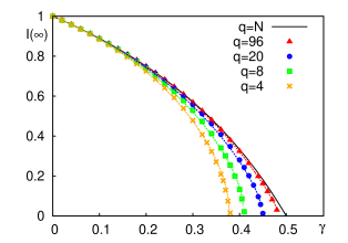
All simulations in the current study are performed on the square of $256\times 256$ individuals, total number of individuals is $N=65536$. The periodic boundary conditions are applied in both directions. Typical times for the system to reach the stationary state vary considerably depending on the value of $I(0)$ and on the proximity to the critical value $\gamma_{c}$, where the relaxation time is the longest. The value of $\gamma_{c}$ depends on $q$ and is defined by the condition that the fraction of infected individuals vanish. Near $\gamma_{c}$, $I(\infty)\sim 0.1$, hence the choice of $I(0)=0.1$ reduces drastically the time needed by the system to reach the stationary state when $\gamma\approx\gamma_{c}$. This choice for $I(0)$ is used in our study and the simulations of $2000$ time-steps are performed at each $\gamma$ ranging from $\gamma=0$ to $\gamma\approx\gamma_{c}$. To avoid locking the system in the state with $I(t)=0$, we allow for at least one infected individual in the system. The dependence of $I(\infty)$ vs curing rate $\gamma$ at various $q$ is shown in Fig. 2. At $q=N$, it follows the solution (5). For $q<N$, the general shape is the same but with reduced critical curing rate $\gamma_{c}$. At $q=4$, we obtain $\gamma_{c}\approx 0.368$, which agree well with the value $\lambda_{c}=1.64872(3)$ found by Sabag et al. [22], where $\lambda_{c}=(1-\gamma_{c})/\gamma_{c}$.

The CA $SIS$ model is characterised by the local infectivity $i_{k}/q$ (6), in contrary to the zero dimensional $SIS$ model, in which case the infectivity is global and equal to $I$. Using the simulation data obtained at $q<N$, the zero dimensional $SIS$ model can be extended to the case of $q<N$ by the following substitution for the infecting rate: $\beta\rightarrow\beta^{\prime}$, where

$$\beta^{\prime}=\beta\frac{\langle i_{k}/q_{k}\rangle}{I}$$

If the averaging is performed in the stationary state, then the dependence of the scaling factor for $\beta^{\prime}$ on $I$ is eliminated. Taking also into account (3), one obtains

$$\beta^{\prime}=\beta\theta(\gamma),\;\;\theta(\gamma)=\frac{\langle i_{k}/q_{k}\rangle_{\mathrm{stat}}}{I}$$ (7)

where “stat” indicates averaging in the stationary state. By solving (2) with the substitution of $\beta$ by $\beta^{\prime}$ according to (7) and taking into account (3), one obtains $I(\infty)$ for the extended zero dimensional $SIS$ model

$$I(\infty)=\frac{1-[1+\theta^{-1}(\gamma)]\gamma}{1-\gamma},\hskip 20.00003pt\gamma<\gamma_{c}.$$ (8)

It yields the following equation for the critical curing rate $\gamma_{c}$:

$$\theta(\gamma_{c})=\frac{\gamma_{c}}{1-\gamma_{c}}$$ (9)

which is not equal to $0.5$ now.

Figure 3: Scaling factor $\theta(\gamma)$ in the stationary state vs curing rate $\gamma$ for the extended zero dimensional $SIS$ model with fixed $q$. Symbols: simulation data, dashed curves: analytic expression, Eq. (10). Fitted values for the exponent $\delta$ are: $0.400$ ($q=4$), $0.319$ ($q=8$), $0.258$ ($q=20$) and $0.175$ ($q=96$).

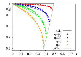
To made the extended zero dimensional $SIS$ model self-contained one needs certain analytic form for $\theta(\gamma)$. It can be obtained by fitting the simulation data obtained at various $q$. The appearance of $\theta(\gamma)$, as shown in Fig. 3, suggests the power law of the form $\sim a(1-\gamma/\gamma_{c})^{\delta}+b$. Constants $a$ and $b$ can be found from the conditions that: (i) at $\gamma=0$ we have the stationary state with $s_{k}=1$ for all individuals, hence $\theta(0)=1$; (ii) at $\gamma=\gamma_{c}$ the value of $\theta(\gamma_{c})$ is given by Eq. (9). Therefore, the only fitting parameter left is the exponent $\delta$. The fitting expression is

$$\theta(\gamma)=\frac{1-2\gamma_{c}}{1-\gamma_{c}}\left(1-\frac{\gamma}{\gamma_{c}}\right)^{\delta}+\frac{\gamma_{c}}{1-\gamma_{c}},$$ (10)

and the results of fitting at selected $q$ are shown in Fig. 3 via dashed lines.

Figure 4: Dependencies of the critical curing rate $\gamma_{c}$ and fitting exponent $\delta$ in Eq. (10) vs $q$ for the extended zero-dimensional $SIS$ model with fixed $q$.

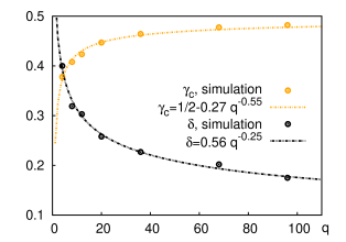
Therefore, the simulations of CA $SIS$ model performed for various neighbourhood size $q$ allow us to extend the zero dimensional $SIS$ model to the case of $q<N$. The solution for the fraction of infected individuals in the stationary state is given by (8). Here the analytic form (10) for $\theta(\gamma)$ is found by fitting the simulation data obtained for CA $SIS$ model. The dependence for the critical curing rate $\gamma_{c}$ and the exponent $\delta$ on $q$ can also be modelled from the simulation data, as shown in Fig. 4. Here the following power laws are used:

$$\gamma_{c}=\frac{1}{2}-Aq^{-u},\hskip 20.00003pt\delta=Bq^{-v},$$ (11)

where $A\approx 0.27$, $u\approx 0.55$, $B\approx 0.56$, and $v\approx 0.25$.

4 Cellular automaton $SIS$ model with random neighbourhood size

It has been pointed out that characterisation of each individual by its own intrinsic infectivity moves the description of the disease spread towards more realistic behaviour [18]. To do so we consider the CA $SIS$ model, where the neighbourhood size $q_{k}$ is random for each $k$th individual at each time step. The evolution of the system of $N$ such individuals is run according to the algorithm

• select random individual $k$

• if $s_{k}=0$ do nothing

• if $s_{k}=1$ then set $s_{k}=0$ with the probability $\gamma$, choose random neighbourood size $q_{k}$ from uniform distribution in $[0;q_{\mathrm{max}}]$ and set $s_{k^{\prime}}=1$ for one of its neighbours with the probability $1-\gamma$

• perform $N$ attempts described above to complete a single time-step

This algorithm is interpreted as the one describing the set of individuals with random implicit mobility. The random neighbourhood size $q_{k}$ is globally bounded by $q_{\mathrm{max}}$. As far as the critical curing rate $\gamma_{c}$ decays with the decrease of $q$ (see, Fig. 4), its value for the model with random $q_{k}<q_{\mathrm{max}}$ will be lower than that for the model with fixed neighbourhood size equal to $q_{\mathrm{max}}$. Both models can be matched to have the same value of $\gamma_{c}$, in which case one requires

$$\frac{1}{q_{\mathrm{max}}}\int_{0}^{q_{\mathrm{max}}}\!\!\!\!\!\!\!\!\gamma_{c}(q^{\prime})dq^{\prime}=\gamma_{c}(q)$$

where the l.h.s. represents the average value for $\gamma_{c}$ for the model with random neighbourhood size bounded by $q_{\mathrm{max}}$, whereas the r.h.s. is the same value of $\gamma_{c}$ obtained for the model with fixed neighbourhood size at particular $q$. Using the analytic fit for $\gamma_{c}(q)$ (11) and performing integration we obtain simple relation between $q_{\mathrm{max}}$ and matching value of $q$

$$q_{\mathrm{max}}=q\left[\frac{1}{1-u}\right]^{\frac{1}{u}}\approx 4.27q.$$ (12)

The simulations performed at the values close to those suggested by the relation (12): $q_{\mathrm{max}}=20$, $36$, $88$ and $420$ match the respective values for $\gamma_{c}$ obtained for $q=4$, $8$, $20$ and $96$ reasonably well, as shown in Fig. 5.

Figure 5: The same as in Fig. 2 but for the CA $SIS$ model with random neighbourhood size at various $q_{\mathrm{max}}$. Values for critical curing rate $\gamma_{c}$ are: $0.376$ ($q_{\mathrm{max}}=20$), $0.426$ ($q_{\mathrm{max}}=36$), $0.462$ ($q_{\mathrm{max}}=88$) and $0.491$ ($q_{\mathrm{max}}=420$).

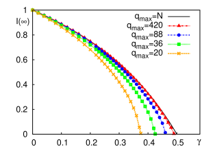
One may conclude that in terms of the critical properties of the stationary state $I(\infty)$, the CA $SIS$ model with random neighbourhood size can be matched well by its counterpart with appropriately chosen fixed value of $q$. $q_{\mathrm{max}}$ and $q$ are related by a simple expression (12) obtained from the fit (11) for $\gamma_{c}$ vs $q$. In the next section we will focus the differences between these two models in terms of the spatial patterns and dynamics of approaching the stationary state.

5 Spatial patterns and evolution of the system towards the stationary state

One of principal advantages of using the CA model defined on a graph is the possibility to analyse spatial patterns of clustered infected individuals, as well as to trace their time evolution [13, 10, 23]. In this study we analyse clustering effects or infected individuals both in the stationary state and when the system approaches it. To define clusters we introduce the cluster neighbourhood size, $q_{C}$, which, in general, does not coincide with the infecting neighbourhood $q$ or $q_{k}$. For the case of $\mathbf{Z}^{2}$ considered here, the value $q_{C}=4$ is used (the nearest neighbours on the square lattice). Thereafter, the clusters are enumerated by index $m$ and the cluster label $c_{k}$ is assigned to each $k$th individual having the meaning of the host cluster for this individual. The following algorithm for the clusters recognition is used:

1. set $\{c_{k}:=0\}$, $m=0$;

2. pick $k$th individual randomly with $s_{k}=1$ and $c_{k}=0$;

3. set $m:=m+1$, $c_{k}:=m$, declare $k$ as a newcomer;

4. loop over the cluster neighbourhoods $\{l\}$ of all newcomers;

5. if $s_{l}=1$ then set $c_{l}:=m$, declare $l$ as a newcomer;

6. repeat steps 4-5 until no newcomers;

7. go to 2.

Alternatively, the Hoshen and Koppelmann [24] algorithm can be used.

At given curing rate $\gamma$ and time instance $t$ we analyse the number of clusters $N_{C}(\gamma,t)$ and a set of their sizes $\{S_{m}(\gamma,t)\}$. Cluster size is given by the number of infected individuals it contains. Reduced number of clusters, as well as average and maximum cluster sizes at given $t$ are given as:

$$n_{C}(\gamma,t) = \frac{1}{N}N_{C}(\gamma,t),$$

$$a_{C}(\gamma,t) = \frac{1}{N}\langle S_{m}(\gamma,t)\rangle_{m},$$

$$m_{C}(\gamma,t) = \frac{1}{N}\max\{S_{m}(\gamma,t)\}.$$

Their time averages performed in the stationary state are denoted as $n_{C}(\gamma)$, $a_{C}(\gamma)$ and $m_{C}(\gamma)$, respectively.

Figure 6: Reduced average cluster size $a_{C}(\gamma)$, maximum cluster size $m_{C}(\gamma)$ and reduced number of clusters $n_{C}(\gamma)$ vs curing rate $\gamma$ in the stationary state. (a) CA $SIS$ model with fixed neighbourhood size $q$ indicated in the figure; (b) CA $SIS$ model with random neighbourhood size at various $q_{\mathrm{max}}$ indicated in the figure. Characteristic values of $\gamma$ that separate various clustering regimes are denoted as $\gamma^{+}$, $\gamma^{*}$ and $\gamma_{c}$ (critical curing rate).

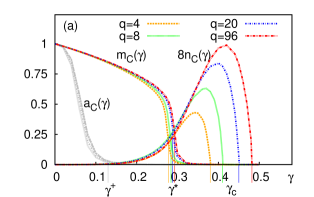
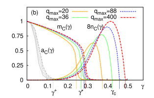
The behaviour of these averages is shown in Fig. 6 for both cases of CA $SIS$ model with fixed $q$ [frame (a)] and CA $SIS$ model with random $q$ [frame (b)]. The set of values $q=4,8,20,96$ used for the model with fixed $q$ matches the respective set of values $q_{\mathrm{max}}=20,36,88,400$ for the model with random $q_{k}$ in terms of close respective values of $\gamma_{c}$, as discussed in Sec. 4, Eq. (12). For both types of models one can distinguish three following regimes:

1. single large cluster ($\gamma<\gamma^{+}$): $n_{C}(\gamma)\sim 0$, $a_{C}(\gamma)>0$, $0.9<m_{C}(\gamma)<1$;

2. large + small clusters ($\gamma^{+}<\gamma<\gamma^{*}$): $0<n_{C}(\gamma)<2$, $a_{C}(\gamma)\sim 0$, $0.25<m_{C}(\gamma)<0.9$;

3. small clusters only ($\gamma^{*}<\gamma<\gamma_{c}$): $n_{C}(\gamma)$ peaks, $a_{C}(\gamma)\sim m_{C}(\gamma)\sim 0$.

The value of $\gamma^{+}$ is defined approximately, whereas $\gamma^{*}$ is the inflection point for the $m_{C}(\gamma)$. The regimes (a)-(c) are illustrated in the series of snapshots shown in Fig. 7 that are obtained for the smaller system of $60\times 60$ individuals.

Figure 7: Snapshots with colour-coded clusters of infected individuals for CA $SIS$ model with fixed neighbourhood size $q=4$. Susceptible individuals are not shown. (a)-(c) illustrate respective clustering regimes described in the text.

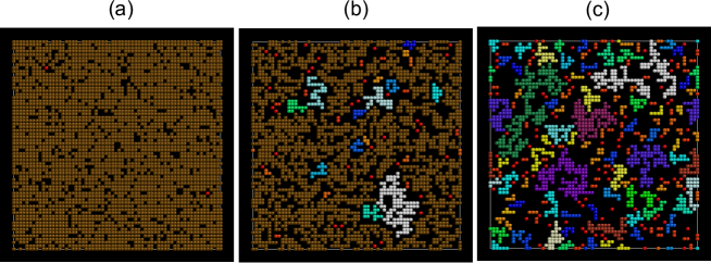
The presence of these regimes indicates that besides the phase transition that occurs at $\gamma\to\gamma_{c}$, where $I(\infty)$ vanishes, there is another transition which takes place earlier, at $\gamma\to\gamma^{*}$, where the size of the largest cluster of infected individuals decreases down to zero. At $\gamma^{*}<\gamma<\gamma_{c}$, only small disconnected clusters are to be found [regime (c) above]. The position of this transition, given by $\gamma^{*}$, is found to be weakly dependent on $q$ for the CA $SIS$ model with fixed $q$ [Fig. 6 (a)]. However, despite matching both models via their respective values of $\gamma_{c}$, their respective values of $\gamma^{*}$ do not match. This is especially evident for the cases of $q_{\mathrm{max}}=20$ vs $q=4$ and $q_{\mathrm{max}}=36$ vs $q=8$. In the model with random implicit mobility ($q_{\mathrm{max}}=20$ and $36$) the maximum cluster size vanishes at lower curing rate $\gamma$ when compared to the model with fixed implicit mobility ($q=4$ and $8$). Therefore, the randomness in the neighbourhood size $q_{k}$ promotes stronger splitting of infected individuals into separate clusters. The higher maximum values of $n_{C}(\gamma)$ occuring within the interval $\gamma^{*}<\gamma<\gamma_{c}$ for the cases $q_{\mathrm{max}}=20$ and $36$ as compared to the respective cases $q=4$ and $8$ also supports this conclusion.

Figure 8: Time evolution of the reduced number of clusters $n_{C}(\gamma,t)$ and the fraction of infected individuals $I(\gamma,t)$ for the CA $SIS$ model with fixed neighbourhood size $q$ indicated in the figure. (a) simulations at respective values of $\gamma$ that lead to $I(\infty)=0.9$ for each $q$; (b) the same for $I(\infty)=0.7$; (c) the same for $I(\infty)=0.5$.

Figure 9: The same as in Fig. 8 except for the CA $SIS$ model with random neighbourhood size $q_{k}\leq q_{\mathrm{max}}$ indicated in the figure.

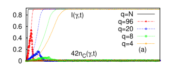
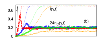
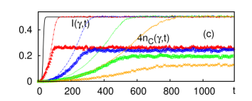
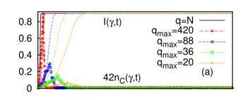
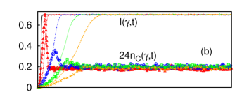
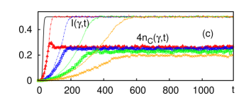
We will consider now the evolution of relevant properties towards the stationary state in both models. To this end the series of runs are performed each started from the initial configuration containing a single infected individual. These series are split into three sets: (a) very low curing rate; (b) low curing rate; and (c) moderate curing rate. Each set contains a number of runs performed for both models at various values of $q$ and $q_{\mathrm{max}}$, respectively. The curing rate $\gamma$ is chosen individually for each run from the condition that the stationary state with $I(\infty)=0.9$, $0.7$, and $0.5$ is reached when the run belongs to (a), (b), and (c) set, respectively. The evolution of the instant fraction of infected individuals $I(\gamma,t)$ and reduced number of clusters $n_{C}(\gamma,t)$ are plotted vs time $t$ for both models in Figs. 8 and 9, respectively. The solution (5) for $I(\gamma,t)$ obtained for the zero dimensional $SIS$ model is also shown and is marked via $q=N$.

Within each set, (a), (b), or (c), for the model with fixed neighbourhood size $q$, the increase of $q$ leads to the reduction of a timescale for the system to reach the stationary state, monitored via behaviour of $I(\gamma,t)$ (see, Fig. 8). Such effect is to be expected, as far as the increase of $q$ is interpreted in terms of enhancement of the implicit mobility, which promotes faster spatial spread of the infection. The fastest infecting dynamics is, obviously, achieved within the zero dimensional $SIS$ model corresponding to the ideally mixed case [5, 6, 7, 18]. Upon introducing random neighbourhood size $q_{k}$, the infecting dynamics also speeds-up when compared to the results of respective matching runs performed at fixed $q$ (compare Figs. 8 and 9). The speed-up ranges from about $1.5$ to $2$ times depending on the particular set, (a), (b), or (c).

The evolution of spatial patterning also demonstrates marked dependence on the model type and the parameters of the run. In particular, for the case of fixed $q$ and moderate curing rate [see, Fig. 8, (c)], the reduced number of clusters $n_{C}(\gamma,t)$ approaches its stationary value monotonically from below. However, the behaviour is different at very low and low curing rates [frames (a) and (b)]. In these cases, at larger neighbourhood sizes, $q\geq 8$, there is a pronounced maximum in the shape of $n_{C}(\gamma,t)$ curve, approximately a mid-way to the stationary state. With the increase of $q$ its height increases. The explanation for the presence of this maximum is the follows. At the early stage the system is mostly uninfected and for larger infection range the newly infected individuals will be formed at some distance from existing infected ones thus increasing the number of separate clusters $n_{C}(\gamma,t)$. However, at a mid-way to the stationary state about half of the system is already infected and newly infected individuals begin to link the existing clusters, thus reducing the number $n_{C}(\gamma,t)$. Similar behaviour is also seen within the model with random $q_{k}$ (shown in Fig. 9), where even higher maxima are observed when compared to matching cases of the model with fixed $q$. Therefore, the introduction of the randomness in the neighbourhood size enhances the hill-like shape in the evolution of the number of clusters $n_{C}(\gamma,t)$. At very low curing rate [frame (a)] the peaks are observed for all $q_{\mathrm{max}}$ being considered.

Therefore, the dynamics of spatial patterning for infected individuals is found to depend strongly on the model type and the parameters of the run. When the initial state comprises almost healthy system (save for one individual), then for the contact-process-like infection spread, $q=4$, the grows of a number of infected clusters towards its stationary value is always monotonic. With the increase of the neighbourhood size, $q>4$, this behaviour changes and the number of clusters shows a pronounced maximum about a mid-way towards its stationary value. This type of behaviour is getting more pronounced for the model with random neighbourhood size.

6 Conclusions

In the present work, we study the $SIS$ model on geometric graph obtained from $\mathbf{Z}^{2}$. To each vertex the individual is attached with two possible states: susceptible or infected. Two options are considered for the neighbourhood size $q$, namely: the fixed $q$; and that taken at random at each step and for each individual $q_{k}$ globally bounded by $q_{\mathrm{max}}$. The neighbourhood size is interpreted as the level of individuals’ implicit mobility. The evolution of the system of $N$ individuals is run according to the asynchronous cellular automata algorithm.

The stationary states are studied first, where we concentrated on the phase transition like behaviour for the ratio of infected individuals $I(\infty)$ which vanishes at the critical curing rate $\gamma=\gamma_{c}$. For the model with fixed $q$, with the increase of $q$, $\gamma_{c}$ increases towards the value $0.5$ characteristic for the zero dimensional $SIS$ model, which corresponds to the case of $q=N$. The simulation data obtained at a range of $q$ is used then to extend the solution for the zero dimensional model to cover the case $q<N$. Simple power-law model form is found for $\gamma_{c}$ as the function of $q$. Close match is found for the phase transition like behaviours of the models with fixed $q$ and random $q_{k}$ bounded by $q_{\mathrm{max}}$ when $q$ and $q_{\mathrm{max}}$ obey certain relation.

In the stationary state we found three distinct regimes of spatial patterning of infected individuals depending on the curing rate $\gamma$: (a) single cluster; (b) large+small clusters; and (c) small clusters only. The phase transition like change between (b) and (c) occurs at $\gamma^{*}$, the inflection point for the size of the largest cluster. The value of $\gamma^{*}$ is found to be weakly dependent on $q$ for the fixed neighbourhood size model but markedly dependent on $q_{\mathrm{max}}$ for the model with random neighbourhood size. It is found that randomness in $q_{k}$ promotes splitting of the largest cluster at lower $\gamma$ as compared to the case of matched case with fixed $q$.

Both the increase of the neighbourhood size and its randomness reduce the time needed by the system to reach the stationary state when simulation is started from the almost healthy state. This is understood in terms of the relation between the neighbourhood size and the individuals’ implicit mobility. The type of evolution of spatial patterning also demonstrates marked dependence on the model type and the parameters of the run. For the contact-process-like infection spread, $q=4$, the grows of a number of infected clusters towards its stationary value is always monotonic. With the increase of the neighbourhood size, $q>4$, this behaviour changes and the number of clusters shows a pronounced maximum about a mid-way towards its stationary value. This type of evolution, which involves the initial built of a huge number of separated clusters and their following merge into larger ones, is getting more pronounced for the model with random neighbourhood size.

This study, performed for a relatively simple $SIS$ model can be extended towards more complex models involving latency, immunity, other types of graphs and memory effects.

7 Acknowledgements

This work was supported by the International Research Staff Exchange Scheme grant “Structure and Evolution of Complex Systems with Applications in Physics and Life Sciences” STREVCOMS-612669 within the 7th European Community Framework Program.