∎
11email: {tagarelli,rinterdonato}@dimes.unical.it
Time-aware Analysis and Ranking of Lurkers in Social Networks ††thanks: An abridged version of this paper appeared in ASONAM14 .
Abstract
Mining the silent members of an online community, also called lurkers, has been recognized as an important problem that accompanies the extensive use of online social networks (OSNs). Existing solutions to the ranking of lurkers can aid understanding the lurking behaviors in an OSN. However, they are limited to use only structural properties of the static network graph, thus ignoring any relevant information concerning the time dimension. Our goal in this work is to push forward research in lurker mining in a twofold manner: (i) to provide an in-depth analysis of temporal aspects that aims to unveil the behavior of lurkers and their relations with other users, and (ii) to enhance existing methods for ranking lurkers by integrating different time-aware properties concerning information-production and information-consumption actions. Network analysis and ranking evaluation performed on Flickr, FriendFeed and Instagram networks allowed us to draw interesting remarks on both the understanding of lurking dynamics and on transient and cumulative scenarios of time-aware ranking.
Keywords:
lurking behavior time-aware lurker ranking LurkerRank algorithms newcomers inactive users responsiveness preferential attachment lurker trends and clustering topical evolution patterns1 Introduction
Lurking is a widely common behavior in online users, which is usually associated with definitions of nonparticipation, infrequent or occasional posting and, more generally, with observation, and bystander behavior NonneckeP00 ; PreeceNA04 . As a fundamental premise, it should be noted that lurkers should not be trivially regarded as totally inactive users, i.e., registered users who do not use their account to join an online community; rather, a lurker can be perceived as someone who gains benefit from other’s information and services without significantly giving back to the online community.
The main general reasons behind the multifaceted nature of this kind of user behavior are well explained in social science, based on various motivational factors, such as environmental, commitment, quality requirements, and individual factors Sun+14 . In general, lurkers represent an enormous potential in terms of social capital, because they acquire knowledge from the online community but never or rarely let other people know their opinions. Lurking can indeed be expected or even encouraged because it allows users to learn or improve their understanding of the etiquette of an online community before they can decide to provide a valuable contribution over time Edelmann13 . Within this view, a major goal is to de-lurk those users, i.e., to encourage lurkers to more actively participate in the online community life: indeed, even though a proper amount of lurkers is acceptable for a large-scale social environment, too many individuals of that kind would impair the virality of the online community.
However, a complete characterization of lurkers has represented a controversial issue in social science and human-computer interaction research Edelmann13 , which has consequently posed several challenges in (quantitatively) analyzing lurking in online social networks (OSNs). Despite the fact that lurkers represent the large majority of members in an OSN, little research in computer science has been done that considers lurking as a valid and worthy-of-investigation form of online behavior. In SNAM14 ; ASONAM , we fill a lack of knowledge on the opportunity of analyzing lurkers in OSNs, and on the important implications that the detection of lurkers can have on a deeper understanding of the feelings in an online community. We addressed the previously unexplored problem of ranking lurkers in an OSN, by introducing a topology-driven lurking definition and proposing a computational framework that offers various solutions to the ranking of lurkers. However, a limitation of the study in SNAM14 ; ASONAM is that it does not deal with temporal information to enhance the understanding and ranking of lurkers in an OSN.
Online social environments are highly dynamic systems, as individuals join, participate, attract, cooperate, and disappear across time. This clearly affects the shape of the network both in terms of its social (followship) and interaction graphs jeong2003measuring ; KumarNT06 ; leskovec2009meme ; budak2011structural ; lehmann2012dynamical ; WilsonSPZ12 ; de2013analyzing ; BerlingerioCGMP13 . Moreover, everybody agrees on the stance that users normally look for the most updated information, therefore the timeliness of users and their relations become essential for evaluation YuLL04 ; BerberichVW05 ; Smyth05 ; LangW13 ; JiangWWSHDZ13 . Like any other user, lurkers as well may be interested not only in the authoritative sources of information, but also in the timely sources.
Research on temporal network analysis and mining strives to understand the driving forces behind the evolution of OSNs and what dynamical patterns are produced by an interplay of various user-related dimensions in OSNs. Dealing with the temporal dimension to mine lurkers appears to be even more challenging. Yet, it’s also an emergent necessity, as users in an OSN naturally evolve playing different roles, showing a stronger or weaker tendency toward lurking at different times. Moreover, as temporal dimension in an OSN is generally examined in terms of online frequency of the users, it’s important to take into account that lurkers may have unusual frequency of online presence as well as unusual frequency of interaction with other users.
Contributions.
Our contributions in this work are twofold. First, we provide insights into the understanding of lurkers from various perspectives along the time dimension in an OSN environment. We conduct different stages of temporal analysis of lurking behaviors, focusing on two macro aspects: how lurkers relate to other types of users in the network, and how patterns of lurking behaviors evolve over time.
Second, we overcome the time-related limitation of previous formulations of lurker ranking methods. To this purpose, we model different temporal aspects concerning both the production and consumption of information, by introducing novel measures of freshness and activity trend, at user and at user-interaction level. These measures are key ingredients in the proposed time-aware lurker ranking methods, for which we develop two approaches: a time-transient based ranking approach, which is restricted to a particular snapshot graph of the network, and a time-cumulative based ranking approach, which encompasses a sequence of snapshots based on a time-evolving definition of freshness and activity functions.
We structure our work into seven research questions (Q1 - Q7), which are summarized as follows.
-
•
Lurking is often related to inactive behavior or to inexperienced usage of the network services at a given time. Therefore, we aim at unveiling whether and to what extent there exists any correspondence between lurkers and zero-contributors (Q1), and between lurkers and newcomers (Q2). From a different perspective, we want also to understand whether lurkers create preferential relations with active users (Q3).
-
•
Responsiveness, i.e., the willingness of a user to respond to other users, is a key criterion to measure behavioral dynamics of users in an OSN. We are hence interested in quantifying how frequently lurkers react to the postings of other users (Q4).
-
•
We investigate how lurking trends evolve over time and how these can be characterized using a clustering framework (Q5). Moreover, by involving also the content dimension, we analyze the topical usage behaviors of lurkers and their topic-sensitive evolution patterns (Q6).
-
•
We assess the ability of our proposed time-aware lurker ranking algorithms in providing improved solutions to the lurker ranking problem. We evaluate the impact of the proposed time-transient and time-cumulative based approaches on the ranking performance, and also compare them with a state-of-the-art time-aware ranking algorithm BerberichVW05 (Q7).
Plan of the paper.
The remainder of this paper is organized as follows. Section 2 provides first a short overview of our early work on lurker detection and ranking in OSNs, then focuses on our proposal of time-aware LurkerRank methods. We answer to each of the above stated research questions in Section 3. Section 4 discusses related work, and Section 5 concludes the paper.
2 Time-aware Lurker Ranking
2.1 LurkerRank at a glance
In SNAM14 ; ASONAM , we developed the first formal computational methodology for lurker detection and ranking. We provided well-principled definitions of lurking, introduced a network graph model oriented to the analysis and mining of lurkers, and defined methods to search and rank lurkers in an OSN.
Our initial definition of lurking relies solely on the topology information available in a OSN, modeled as a followship graph. Upon the assumption that lurking behaviors build on the amount of information a user receives, our key intuition is that the strength of a user’s lurking status can be determined based on her/his in/out-degree ratio (i.e., followee-to-follower ratio), and of her/his neighborhood. We report next the topology-driven lurking definition from SNAM14 :
Definition 1 (Topology-driven lurking)
Let denote the directed graph representing an OSN, with set of nodes (users) and set of edges , whereby the semantics of any edge is that is consuming information produced by . A node with infinite in/out-degree ratio (i.e., a sink node) is trivially regarded as a lurker. A node with in/out-degree ratio not below 1 shows a lurking status, whose strength is determined based on:
- Principle I:
-
Overconsumption. The excess of information-consumption over information-production. The strength of ’s lurking status is proportional to its in/out-degree ratio.
- Principle II:
-
Authoritativeness of the information received. The valuable amount of information received from its in-neighbors. The strength of ’s lurking status is proportional to the influential (non-lurking) status of the ’s in-neighbors.
- Principle III:
-
Non-authoritativeness of the information produced. The non-valuable amount of information sent to its out-neighbors. The strength of ’s lurking status is proportional to the lurking status of the ’s out-neighbors.
The above principles form the basis for three ranking functions that differently account for the contributions of a node’s in-neighborhood and out-neighborhood. We finally provided a complete specification of our lurker ranking models in terms of PageRank-style methods. For the sake of brevity here, and throughout this paper, we will refer to only one of the formulations described in SNAM14 ; ASONAM , which is that based on the full in-out-neighbors-driven lurker ranking, hereinafter dubbed simply as LurkerRank.
Given a node , let us denote with and the set of in-neighbors (i.e., backward nodes) and the set of out-neighbors (i.e., reference nodes) of , respectively. The in-degree and out-degree of are denoted as and , respectively. The following formula gives the LurkerRank for any node :
| (1) |
where is the in-neighbors-driven lurking function:
| (2) |
and is the out-neighbors-driven lurking function:
| (3) |
Moreover, is a damping factor ranging within [0,1], usually set to 0.85. To prevent zero or infinite ratios, the values of and are Laplace add-one smoothed.
2.2 Time-aware LurkerRank methods
In this section we describe our extensions to LurkerRank that account for the temporal dimension when determining the lurking scores of users in the network. We follow two approaches based on different models of temporal graph:
• Transient ranking, i.e., a measure of a user’s lurking score based on a time-static (snapshot) graph model;
• Cumulative ranking, i.e., a measure of a user’s lurking score that encompasses a given time interval (sequence of snapshots), based on a time-evolving graph model.
The building blocks of our methods rely on the specification of the temporal aspects of interest, namely freshness and activity trend, both at user and at user relation level. Freshness takes into account the timestamps of the latest information produced (i.e., posted) by a user, or the timestamps of the latest information consumed by a user in relation to another user’s action. Activity trend models how the users’ posting actions or the responsive actions vary over time. These concepts will be elaborated on in the next section.
2.2.1 Freshness and activity trend functions
Users in the network are assumed to perform actions and interact with each other over a timespan . The temporal domain is conveniently assumed to be . Therefore, the time-varying graph of an OSN is seen as a discrete time system, i.e., the time is discretized at a fixed granularity (e.g., day, week, month).
Freshness.
Let be a temporal subset of interest, being in interval notation of the form , with . For any time , we define the freshness function as:
| (4) |
Function ranges within . Note that we opt for a function with logarithmic decay to ensure, as gets larger, a slower decrease w.r.t. other decreasing functions with values in —for instance, the graph of lies always above the graph of , or of .
Given a user , let be the set of time units at which performed actions in the network. The freshness of at a given temporal subset of interest is defined as:
| (5) |
Note that is always defined and positive, for all . Higher values of correspond to more recent activities of w.r.t. .
Activity trend.
The second aspect we would like to understand is the activity trend of a user. Let us first denote with
| (6) |
the time series representing the activity of user over . For every pair , denotes the number of ’s actions at time .
In order to model the temporal evolution of the activity of a user , we employ the Derivative time series Segment Approximation (DSA) GulloPTG09 and apply it to the user’s activity time series . DSA is able to represent a time series into a concise form which is designed to capture the significant variations in the time series profile. For any given time series of length , DSA produces a new series of values, with . The main steps performed by DSA are summarized as follows:
-
•
Step 1 - Derivative estimation: is transformed into , where each value is replaced by its first derivative estimate.
-
•
Step 2 - Segmentation: the derivative time series is partitioned into variable-length segments. Each of the segments aggregates subsequent data values having very close derivatives, i.e., it represents a subsequence of values with a specific trend.
-
•
Step 3 - Segment approximation: each of the segments in is mapped to an angular value , which collapses information on the average slope within the segment.
The DSA series is of the form , such that and , with , where is the -th segment, its length, and the mean of its points.
As a post-processing step, the values of the DSA sequence are normalized within [0,1] by deriving the values . In this way, an increasing (resp. decreasing) trend of activity will correspond to a value within (resp. ). Therefore, we define the activity trend of user (over the whole interval ) as the time sequence:
| (7) |
Given a temporal interval of interest , the activity trend of w.r.t. corresponds to the subsequence of that fits . It is also useful to define the average activity of over , denoted by , as the average of the values within .
Freshness and activity trend of interaction.
The notions of freshness and activity trend for individual users are here extended to model the interaction of any two users at a given time , which corresponds to the directed edge (also here denoted as ) in the snapshot graph containing . The rationale here is that the more recent is an interaction (or the more increasing is its activity trend), the stronger should be the relation . Recall that means that is consuming information at time produced by .
Let us denote with the set of information-production actions of , and with the associated timings. Moreover, let be a set of triplets , such that , and denote the time and the frequency, respectively, at which consumed the ’s post . Note that we have used subscripts p and c to mean “production” and “consumption”, respectively.
According to the above formalism, we define the freshness of interaction w.r.t. as the maximum freshness over the sequence of pairs (production-time, consumption-time) in :
| (8) |
Analogously, we define the activity trend of interaction, based on the DSA model previously used to define the activity trend of user. To this end, given the interaction , we consider the time series representing pairs , where denotes the number of actions at time performed by in response to a specific post by . Then, we compute the activity trend of interaction , denoted with , as the result of the application of DSA to the time series . The definition of is analogous to .
2.2.2 The time-static LurkerRank algorithm
Our first formulation of time-aware LurkerRank is based on a time-static graph model, which contains one single snapshot of the network. Our key idea is to capitalize on the previously proposed functions of freshness and activity to define a time-aware weighting scheme that determines both the strength of the productivity of a user and the strength of the interaction between any two users linked at a given time. To this purpose, we introduce two real-valued, non-negative coefficients to control the importance of the freshness and the activity trend in the weighting scheme.
Given a temporal interval of interest , and coefficients , we define the function in terms of the user freshness and average activity calculated for any user :
| (9) |
By default, the two coefficients are set uniformly as . If is contained into (i.e., ) and the average activity is zero, the value will coincide to the freshness value, which is strictly positive; otherwise, if , the value will equal one. It should be noted that will hence be 1 if either the freshness and average activity are maximum or is not relevant to the timespan over which the user has been active: this is admissible in our theory since we want to exploit information about the user activity only if this is available in a given time interval. The rationale behind the value assigned to a vertex is to add a multiplicative factor that is inversely (resp. directly) proportional, otherwise neutral, to the size of the in-neighborhood (resp. size of the out-neighborhood ) in the formulation of our time-static LurkerRank algorithm.
Analogously to , we define the function in terms of the freshness and average activity of interaction calculated for any such that , as follows:
| (10) |
Compared to Eq. (9), note that the expression in Eq. (10) holds zero if the freshness is zero. This will be clear as we will show the use of in an exponentially negative smoothing term that is present in the definition of our time-static LurkerRank algorithm.
We are now ready to provide our formulation of the time-static LurkerRank algorithm, hereinafter denoted as Ts-LR, which involves both functions and above defined. Time-static LurkerRank shares with the basic LurkerRank formulation the way the in-neighbors-driven lurking term is combined with the out-neighbors-driven lurking term, that is, for any user and temporal interval of interest :
| (11) |
However, the in-neighbors-driven lurking function is now defined as:111Note that, for the sake of simplicity, we have omitted the subscript in the freshness and activity trend functions, in the weighting function as well as in the and functions, since the reference interval of interest is assumed clear from the context. Analogously, we override the function symbols and given in Eq. (1), since they will be never referenced out of the Ts-LR setting.
| (12) |
and the out-neighbors-driven lurking function as:
| (13) |
2.2.3 The time-evolving LurkerRank algorithm
The time-static LurkerRank can work only on a subset of relational data that are restricted to a particular subinterval of the network timespan. Therefore, information on the sequence of events concerning users’ (re)actions is lost as relations are aggregated into a single snapshot. To overcome this issue, we define here an alternative formulation of time-aware LurkerRank that is able to model, for each user , the potential accumulated over a time-window of the contribution that each in-neighbor had to the computation of the lurking score of .
Cumulative freshness and activity functions.
We begin with the definition of a cumulative scoring function which forms the basis for each of the subsequent functions that will apply to the previously defined freshness and average activity at user and interaction level. Intuitively, this cumulative scoring function () should be defined at any time to aggregate all values of a function (defined in ) computed at times less than or equal to , following an exponential-decay model:
| (14) |
Let the timespan of the network graph be partitioned in consecutive sub-intervals . The generic cumulative scoring function has a straightforward translation in terms of user-freshness: if corresponds to the end-time of the span of interest whose latest sub-interval is , we define the cumulative user-freshness function applied to any user to integrate (with exponential decay) all user-freshness values individually obtained at each sub-interval preceding :
| (15) |
Our cumulative user-activity function, we denote with , has similar form. Formally, for every , we have:
| (16) |
The definition of cumulative freshness of interaction, , and cumulative activity of interaction, , at each , and for every , follow intuitions analogous to Eq. (15) and Eq. (16), respectively.
The values yielded by the above defined four functions of cumulative freshness and activity, at user as well as at interaction level, are then normalized and multiplied by the corresponding information in the transient model, that is, for every :
| (17) |
| (18) |
The user-interaction function counterparts have analogous form to Eq. (17) and Eq. (18). Our motivation for adopting a (multiplicative) combination of a normalized cumulative freshness/activity function with a transient freshness/activity function, is that we want to ensure that the freshness/activity information cumulated through times preceding a target time will be valued w.r.t. the actual contribution (in terms of freshness/activity) that the user provides in the OSN at given time .
The time-evolving LurkerRank algorithm, hereinafter denoted as Te-LR, follows a formula that is analogous to the Ts-LR. However, Te-LR adopts new weighting functions, we denote as and , which have the following properties:
- •
- •
3 Temporal Analysis of Lurkers
We present here our multi-faceted, temporal analysis of lurkers along the time dimension. In Section 3.1, we frame seven research questions, which span different problems of interest to our study. We describe the data that will be used for our evaluation in Section 3.2. Then, Sections 3.3–3.9 will contain our answer to each of the stated questions.
3.1 Outline of research questions
Our study of lurkers and lurking behaviors across time is built upon seven research questions, which are stated as follows.
Q1: Do lurkers match zero-contributors? Definitions of lurking are often related to nonposting behavior. Our first research question is aimed at gaining insights into the correspondence between inactive users and lurkers over time. Inactive users are here intended as “zero-contributors”, i.e., users who have never posted or provided a comment/favorite-mark.
Q2: Do lurkers match newcomers? Lurking can depend on a temporary status of learning the etiquette of the community and the proper usage of the services provided by an OSN. This also relates to newcomers, i.e., users that have started to participate in some activity. Therefore, analogously to our first research question, we also analyzed the relation between newcomers and lurkers over time.
Q3: Do lurkers create preferential relations with active users? In the third research question, our goal is to unveil the dynamics of the binding between lurkers and active users, and how this relates to the popularity of the active users.
Q4: How frequently do lurkers respond to the others’ actions? Lurkers can show a limited amount of activity in response to others’ contributions to the community life. We are interested in measuring the distribution of time latency that occurs to observe repeated actions by a user in response to his/her followees (i.e., comments, or favorite-marks).
Q5: How do lurking trends evolve? Our fifth research question focuses on how lurking trends change over time, how they can be grouped together, and whether characteristic patterns may arise to indicate different profiles of lurkers.
Q6: How do topical interests of lurkers evolve? We are also interested in exploring topic-sensitive evolution patterns of lurking behavior. We analyze the topical usage of lurkers, how lurkers change their topical patterns, and whether these changes might differ from those of the other users.
Q7: Can time-aware models improve the ranking of lurkers? In our final research question, we investigate the impact of using our proposed time-transient and time-cumulative ranking models on the quality of lurker ranking solutions. We provide a quantitative analysis of results obtained by our developed time-aware LurkerRank algorithms, with respect to a data-driven evaluation of the ranking performance. We also offer a comparison with a state-of-the-art time-aware ranking algorithm BerberichVW05 .
3.2 Data
We used data from Flickr, FriendFeed and Instagram networks to conduct our analysis. A major motivation underlying our data selection is that we wanted to use datasets that have been previously studied in research and that contain timestamped information on the activities of users and their relationships, including followships, comments, or like/favorite-markings. Flickr dataset was originally collected in 2006-2007 and used in mislove08wosn ; cha2009www , FriendFeed refers to the latest (2010) version of the dataset studied in CelliLMPR10 , while Instagram is our dump recently crawled in 2014, whose user interaction network was used in ASONAM14 . Flickr and FriendFeed have also been selected to be consistent with our previous analysis of lurkers SNAM14 . We refer the reader to the original works that used Flickr and FriendFeed, and to our submission support page available at http://uweb.dimes. unical.it/tagarelli/timelr/ for the description of the Instagram dump.
| data | # nodes | # links | avg | avg | clust. | assorta- |
|---|---|---|---|---|---|---|
| in-deg. | path len. | coef. | -tivity | |||
| averages over time-varying snapshot graphs | ||||||
| Flickr-social | 1,889,102 | 25,265,343 | 13.25 | 4.41 | 0.108 | 0.009 |
| Flickr | 215,429 | 1,483,462 | 6.85 | 4.69 | 0.025 | -0.013 |
| FriendFeed | 6,962 | 64,509 | 5.15 | 5.89 | 0.071 | -0.043 |
| 10,353 | 31,215 | 2.94 | 5.83 | 0.083 | 0.217 | |
| full (static) social graphs | ||||||
| Flickr | 2,302,925 | 33,140,018 | 14.39 | 4.36 | 0.107 | 0.015 |
| FriendFeed | 493,019 | 19,153,367 | 38.85 | 3.82 | 0.029 | -0.128 |
| 54,018 | 963,833 | 17.85 | 4.50 | 0.048 | -0.067 | |
Note that our selected datasets are rather heterogeneous in terms of features concerning user relationships: Flickr contains timestamps of 34.7M favorite markings assigned to the uploaded photos, and also contains (inferred) timings on the user subscriptions. In Instagram, every link between (follower) and (followee) is annotated with the number and timestamp of the ’s comments to media posted by (about 2M comments and 1.7M likes). Analogous to Instagram is the situation in FriendFeed but for information concerning likes (230K) and comments (687K) to posts.
Table 1 summarizes main structural characteristics of the network datasets we used in our evaluation. The table is organized in two subtables. The upper subtable contains statistics on timestamped snapshot graphs averaged over the network-specific timespan, which was binned at month level; more precisely, in order to have uniformly-sized snapshots, we aggregated them on a 28-days (i.e., 4 weeks) basis. Note also that all snapshots refer to interaction subgraphs except the first row in the table which corresponds to the timestamped followship (social) subgraphs of Flickr. The timespans covered by the datasets are 7 months for Flickr (2006/11/02 – 2007/05/17 for the followship subgraphs and 2006/09/08 – 2007/03/22 for the interaction subgraphs), 7 months for FriendFeed (2010/04/09 – 2010/09/30), and 20 months for Instagram (2012/06/28 – 2013/12/18). The lower subtable contains statistics on the full (i.e., static) social graphs of Flickr, FriendFeed and Instagram.
 |
 |
 |
| (a) Flickr | (b) FriendFeed | (c) Instagram |
3.3 Lurkers vs. inactive users
Our first question (Q1) focuses on the relation between lurkers and inactive users, also referred to as zero-contributors.
To answer this question, we initially analyzed how much the set of zero-contributors overlaps with the set of users having an in/out-degree ratio higher than one, here dubbed “potential lurkers”. When considering the static picture of a network dataset, one remark is that the set overlap between zero-contributors and potential lurkers may vary from 12% (favorite-based interaction network in Flickr) to 72% and 95% (comment-based interaction networks in FriendFeed and Instagram, respectively). Moreover, since the relative difference in size of the two sets can vary from one dataset to another, we also computed the overlap ratio w.r.t. the set of potential lurkers, which was found to be 57% on Flickr, 62% on Instagram, and 96% on FriendFeed. There are hence clues that the overlap (or overlap ratio) would be relatively smaller when favorite/like interactions are taken into account, that is, potential lurkers are more likely to behave similarly to inactive users when activity is regarded in terms of commenting.
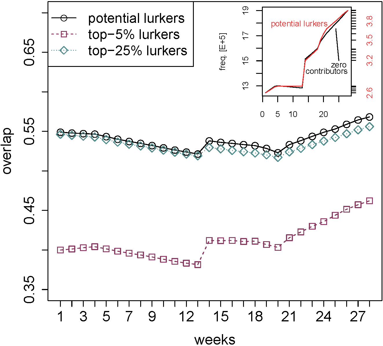
We further investigated how the relation between inactive and lurking users evolves over time. In this analysis, we also included the set of top-ranked users obtained by our LurkerRank. Figure 1 shows the temporal trends of overlap ratios w.r.t. potential lurkers, top-5% and top-25% ranked lurkers, on Flickr. Interestingly, the overlap ratios remain rather unaffected over time, despite the jump in frequency at the 14-th week (displayed in the inset). The distribution of top-5% ranked lurkers is always above the other two series (up to 0.15), which in turn roughly match. Note that in the inset, the distributions of potential lurkers and zero-contributors actually follow close trends, although they are scaled differently (on one order of magnitude).
|
|
|
|
|---|---|---|---|
| (a) Flickr | (b) FriendFeed | (c) Flickr | (d) FriendFeed |
3.4 Lurkers vs. newcomers
Similarly to the previous analysis, in our second research question (Q2), we investigated whether and to what extent lurkers and newcomers can overlap at any given time in our evaluation networks.
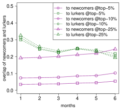
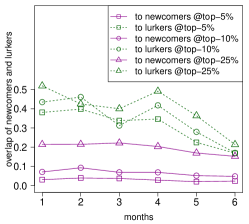
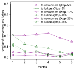
To this end, we assumed that a user is regarded as a newcomer at time if, at any time , s/he was not involved in any interaction with other users, while lurkers were identified at each time . Figure 2 shows, for each dataset and relating top-LurkerRank solutions at 5%, 10% and 25%, two series over a six-month timespan: the fraction of newcomers that were recognized as lurkers (solid lines) and the fraction of lurkers that were also newcomers (dashed lines).
In the case of interactions as Flickr favorite-markings actions, shown in Fig. 2(a), we observe that the fraction of lurkers matching newcomers varies from about 30% down to 20%, following the same trend over the timespan regardless of the top-% selected from the LurkerRank solution; by contrast, the trend of the fraction of newcomers matching lurkers is more constant (and slightly increasing) over the timespan, achieving values below 10%, for top-5% and top-10% lurkers, and around 20% for top-25% lurkers.
Considering a comment-based interaction scenario, shown in Fig. 2(b)-(c), again the trend of the fraction of newcomers matching lurkers looks roughly constant over time. As concerns the fraction of lurkers matching newcomers, it is within 50-20% in FriendFeed, but below 10% on average in Instagram.
We tend to believe that the difference in matching (between lurkers and newcomers) among the various scenarios might be explained due to inherent characteristics of an OSN, rather than to the type of interaction (as previously observed in the evaluation of inactive users versus lurkers). Nevertheless, we would like to point out that our research objective in comparing lurkers with newcomers is consistent with previous research focused on the analysis of newcomers’ behavior in an OSN: in fact, as found by Burke et al. BurkeML09 , newcomers’ behavior can be explained by examining how they tend to be engaged in content production activities by observing their friends’ actions. This is nothing less than a form of Bandura’s observational learning Bandura , i.e., learning through being given access to the learning experiences of other users; as widely studied in social science and human-computer interaction, observational learning and lurking are related to each other Edelmann13 ; Sun+14 .
3.5 Preferential attachment
Our third research question (Q3) focuses on understanding whether relations between lurkers and the active users they are linked to can be explained in terms of power law and preferential attachment. To this purpose, we selected the set of lurkers and the set of active users respectively from the top and the bottom of the LurkerRank solution.
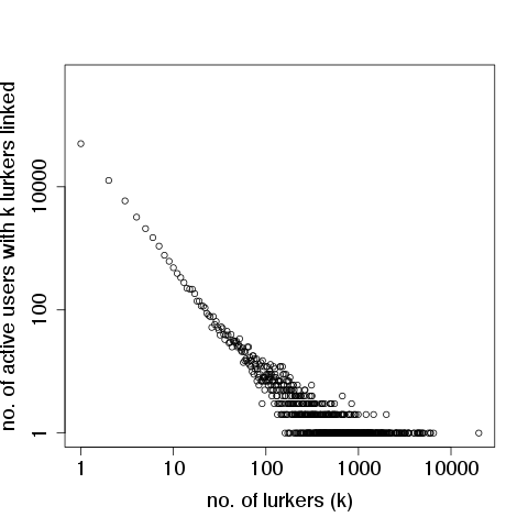
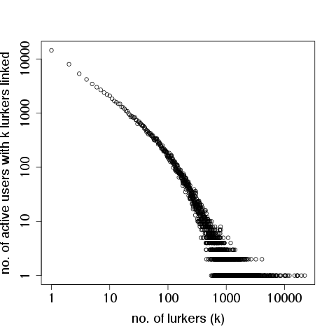
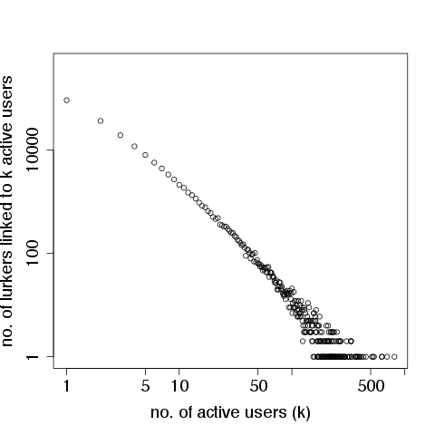
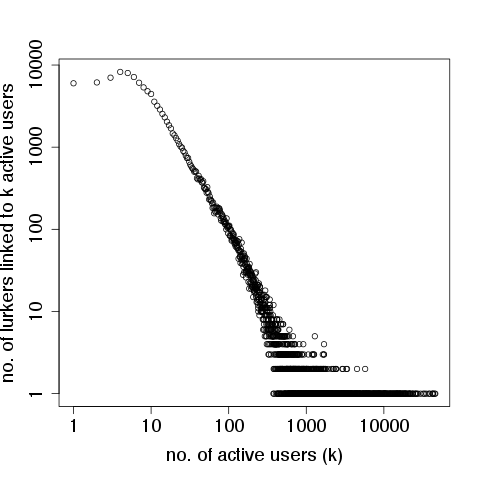
We first investigated whether the probability of observing active users with a certain degree of attached lurkers, and vice versa, can be predicted by a power-law. Figure 3 shows the distribution of lurkers as a function of the degree of attached active users, and also for the distribution of active users, obtained on the Flickr and FriendFeed followship graphs, using the top-25% and bottom-25% of the LurkerRank solution. We computed the best fit of a power-law distribution to the observed data, and assessed the statistical significance of the fitting by a Kolmogorov-Smirnov test. From the figure it can be noted that the plots follow a power-law behavior. The exponents of the fitted power-law distributions are 1.725 () and 1.363 () for Flickr (Fig. 3(a) and (c), resp.), 2.015 () and 1.679 () for FriendFeed (Fig. 3(b) and (d), resp.). In all cases, the power-law fitting is statistically significant, with Kolmogorov-Smirnov test statistic (resp. -value) of 0.0236 (resp. 0.8006) for Fig. 3(a), 0.0396 (resp. 0.7662) for Fig. 3(c), 0.0516 (resp. 0.9946) for Fig. 3(b), and 0.0546 (resp. 0.9161) for Fig. 3(d).
Our main goal to answer question Q3 is to try explaining the relation between lurkers and active users in terms of preferential attachment, that is, we hypothesize that lurking connections are attached preferentially to active users that already have a large number of connected lurkers. Following the lead of mislove08wosn , we studied two separate cases of “attachment”, which differently rely on a user’s in-neighborhood or out-neighborhood. However, in our context, such a type of analysis becomes more complicated since nodes (and their neighborhood) must be selected according to their different status as either lurker or active user. Intuitively, two cases of preferential attachment can be considered, namely: new connections received by active users for any lurkers, and new connections produced by lurkers for any active users.
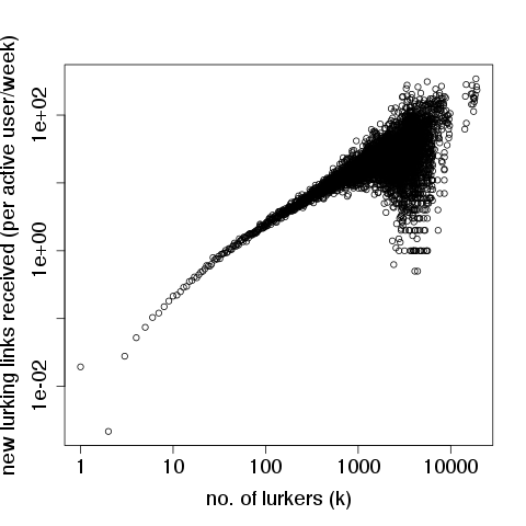
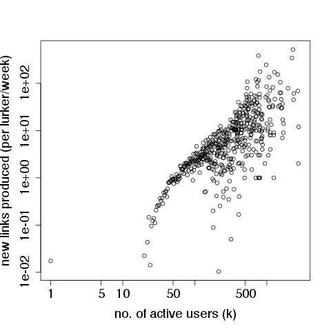
We initially investigated the two cases of preferential attachment according to the timestamped followship information in a network. Figure 4 shows results obtained on Flickr, averaged per user and per week, for each . It can be noted that the number of lurkers shows a good linear correlation with the average number of new links received by active users (left-hand side of Fig. 4): the least-squared-error linear fit has a slope of 0.00836, which means that on average active users receive per week one new connection from lurkers for every 120 lurker-followers that they already have. By contrast, given a correlation of -0.11, no linear trend exists when studying the new connections produced by lurkers for any active users (right-hand side of Fig. 4). Therefore, it is unlikely that lurkers following a high number of active users will create new connections towards other active users.
|
|

|
|
|---|---|
| (a) Instagram | (b) FriendFeed |
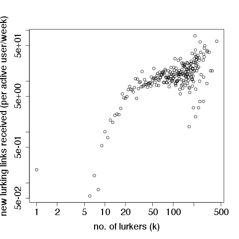
We further explored the preferential attachment evaluation between lurkers and active users focusing on timestamped interaction information in a network. Specifically, we considered user interaction based on likes or comments in Instagram, and on comments in FriendFeed. Figure 5 shows results obtained on the two datasets that concern the correlation between the number of lurkers () and the average number of new links received by active users for any given , on a weekly basis. Correlation is moderate (0.34 on Instagram, 0.52 on FriendFeed), while, in terms of least-squared-error linear fit, the two distributions have a slope of 0.00570 (Instagram) and 0.06585 (FriendFeed), which correspond to having one new interaction (i.e., posted comment) from lurkers per active user and week for every 176 and 15, respectively, lurkers that have already interacted. However, compared to the analogous situation on weekly-aggregated Flickr followship networks in the left-hand side of Fig. 4, both the distributions in Fig. 5 have lower correlation and also lower size, which can be explained since temporal information about user interactions (i.e., likes/comments) in both networks is relatively sparse with respect to that about followships. In effect, by aggregating interaction relationships on a monthly basis, correlation increases (0.47 on Instagram, 0.66 on FriendFeed), along with a decrease of the amount of preferential attachment (one new interaction from lurkers per active user and month for every 51 and 4 interacting lurkers on Instagram and FriendFeed, respectively). Finally, concerning new connections produced by lurkers for any active users, we observed very sparse distributions with null correlation, on both datasets and regardless of the temporal grain of the aggregated networks. This means that lurkers, which have a higher number of active users as recipients of their likes/comments, are not more prone to have new interactions with other active users.
(a) Flickr
(b) Instagram
(a) FriendFeed
(b) Flickr
(c) Instagram
3.6 Responsiveness
Concerning question Q4, we aim at estimating how frequently lurkers react to the postings of other users.
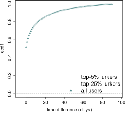
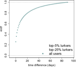
We examined the distribution of time differences (in days) between any two consecutive responsive actions made by a user w.r.t. a post created by her/his followees. Figure 6 shows the empirical cumulative distribution functions over the first 90 days, for comments on Instagram and for favorites on Flickr. Each of the plots in the figure compares the distributions obtained for top-5% and top-25% lurkers with the distribution corresponding to all users in the network.
We observe that the lurkers’ responsiveness generally takes several days, or weeks, although the latency between any two consecutive responsive actions may significantly vary in the two networks. Focusing on the 80% of responses (i.e., 0.8 on the -axis of the plots), the latency is up to 18 days in Flickr, with no evident difference regarding the fraction of top-ranked lurkers considered; by contrast, in Instagram, the top-25% lurkers have an average responsiveness of more than three weeks, which takes even longer (40 days) in the case of top-5% lurkers. Moreover, compared with the responsiveness of all users, lurkers tend to react more slowly, up to 20 days more in Instagram; however, the gap with respect to all users is only of few days in both networks when the fraction of top-ranked lurkers is large (25%). Thus, more time-consuming responsive actions, like comments in Instagram, would explain not only the increase in the the lurkers’ responsiveness but also the relative difference with the generic case of all users.
| LDA topic ids | topic-set | main descriptors (i.e., media tags) of topic-set | subnetwork- |
| label | induced size | ||
| 0, 6, 10 | nature | sky, sunset, whpflowerpower, whpsignsoftheseason, clouds, nature, landscape, | 8,185 |
| sea, beach, flowers, water, trees, hinking, summer, fall, autumn | |||
| 12, 14 | architecture | whpstraightfacades, architecture, building, instaworld_shots, streetphotography, | 2,884 |
| spain, madrid, paris, france, london, sicily, design, arquitectura, youmustsee | |||
| 13 | fun | love, me, swag, lol, fun, like, awesome, cool, happy, food | 1,314 |
| 16 | pets | whppetportraits, cats, caturday, catstagram, dog, cute, pets, kitty, catsofinstagram, petsofinstagram | 3,124 |
| 19 | video | whpmovingphotos, whpreplacemyface, whpbigreveal, whpfilmedfromabove, instavideo, | 3,062 |
| video, whpmovingportrait, movies, videogram, instagramvideo | |||
| 1, 2, 7 | miscellanea | whpthroughthetrees, ig_captures, whpmyhometown, whpliquidlandscape, whpemptyspaces, whpmotherlylove, | 16,573 |
| whpthanksdad, whpstraightfacades, whpmyfavoriteplace, whpfirstphotoredo, whpstrideby | |||
| 8, 18 | travel | worldunion, whpmyfavoriteplace, travel, world_shotz, worldcaptures, worldplaces, igworldclub | 1,200 |
| 3, 4, 5, 17, 11 | attention-seeking | instagood, instamood, photooftheday, pleasecomment, pleaseshoutout, teamfollowback, | 5,794 |
| igers, picoftheday, instadaily, bestoftheday, webstagram, iphonesia, igdaily | |||
| 9, 15 | photo art | whpsilhouettes, whpselfportrait, whplookingup, whpreflectagram, selfie, | 11,882 |
| blackandwhite, whpbehindthelens, whpstilllife, silhouette, bnw, monochrome |
3.7 Temporal trends and clustering
In our fifth research question (Q5), we analyze how lurking trends evolve, focusing on unveiling the structures hidden in such evolving trends.
We pursued this goal as a task of clustering of time series representing the users’ lurking profiles. The basis for this clustering analysis lies in repeatedly applying our LurkerRank to successive snapshots of a network dataset. Since the snapshots can vary in size, LurkerRank scores were first normalized to be comparable across different times. We then generated a time series of the normalized LurkerRank scores for every user in the dataset. The resulting set of time series was the input for our clustering task.
We adopted a soft clustering approach to group the time series of LurkerRank scores. This implies that a time series is allowed to obtain fuzzy memberships to all clusters. Our choice is motivated by suspicion that the natural clusters to be detected in this kind of time-course data could not be well-separated, rather they could be frequently overlap. A suitable method to detect clusters in this kind of data is based on fuzzy c-means clustering. We used a particularly efficient implementation, provided by the Mfuzz R-package tool,222http://www.bioconductor.org/packages/release/bioc/html/Mfuzz.html. based on minimization of the weighted square error function. Note that since the clustering is performed in Euclidean space, the time series were standardized to have a mean value of zero and a standard deviation of one. This preprocessing step ensures that series with similar variations are close in Euclidean space. As concerns the setting of the fuzzifier and the number of clusters required by the clustering algorithm, we follow the methodology suggested in SchwammleJ10 , and summarized in our submission support page available at http://uweb.dimes.unical.it/tagarelli/timelr/.
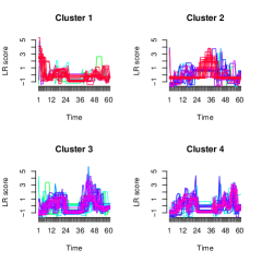
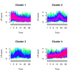
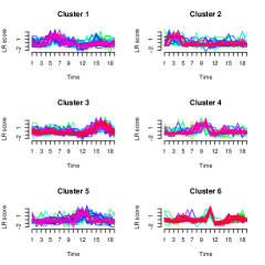
Figure 7 shows some of the clustering results we obtained on the evaluation datasets. For this analysis, we initially selected the top-25% lurkers of the snapshot at time zero, then kept only those users appearing in at least 50% of the subsequent snapshots. Results correspond to different scenarios, both in terms of time-granularity (which impacts on the time series length) and type of relation (i.e., comments, favorite-marks, likes plus comments) underlying the graphs from which the time series were generated. Note that the membership values of time series are color-encoded in the plots, which facilitates the identification of temporal patterns in the clusters.
It can be noted from the figure that some cases are characterized by quite evident trends. For instance, on Flickr, cluster#2 groups lurkers whose behavior (lurking scores) evolves in the form of a series with an initial plateau followed by an increasing ramp and then a decreasing ramp, finally by a new stagnation trend. Similar is the situation depicted by cluster#3 on Flickr. On FriendFeed, clusters#1-#3-#4 present a more or less marked period of roughly constant lurking behavior between the 24th and 36th weeks, along with various peaks in the heads or tails of the series, which would hint at particularly critical (passive) periods of lurking. In general, more time-consuming actions (i.e., comments on Instagram, like+comments on FriendFeed) tend to correspond to trends that present sharper upward/downward shifts, and to clusters with more noisy data. Finally, note that except for cluster#1 on Flickr, lurking series do not tend to group into decreasing trends, which would suggest that lurkers are not likely to spontaneously “de-lurk” themselves, i.e., to turn their behavior into a more active participation to the community life.
3.8 Topical evolution
 |
 |
 |
 |
| (a) | (b) | (c) | (d) |
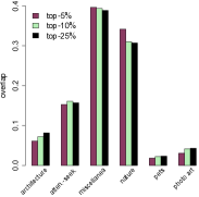
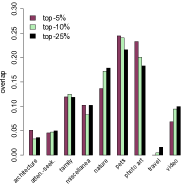
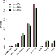
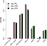
Our six research question (Q6) concerns the analysis of topic-sensitive evolution patterns of lurking behavior. This involves a characterization of the topical usage of lurkers, of how their topical patterns evolve and whether these may differ from those of the other users.
To answer this question, we employed a statistical topic model to learn the topics of interest exhibited by the users. More specifically, we used an efficient implementation provided in the gensim library333http://radimrehurek.com/gensim/. of the well-known Latent Dirichlet Allocation (LDA) BleiNJ03 . For the sake of brevity, we focus here on the presentation of results that we obtained on the Instagram dataset, for which we regarded all media of a user as a single document and the tags assigned by users to their media as document features. We filtered out tags occurring in less than five documents or in more than 75% of the documents in the collection. We tested our topic model with 5 to 50 latent topics, in increments of 5, executing up to 100 iterations; upon a manual inspection of the description of topics learned by the LDA models, we adopted the model with 20 topics as the most “interpretable” one. Our decision was indeed taken based on obtaining a topic description as sharp and rich as possible in terms of both characteristic and discriminating features. We remark that the topics extracted by our selected LDA model are consistent with a previous study on topical interests that was performed on a similar dump of the Instagram media dataset HT14 . That study showed how the most popular tags in Instagram concern a limited number of categories, or coarse-grain topics, which include: nature, travels, photography-related technical aspects, usage of popular applications for photo/video editing and publishing (e.g., Latergram, VSCO Cam), attention-seeking and microcommunity-focused tags (e.g., #photooftheday, #igmaster, #justgoshoot, #iphonesia).
We used the learned 20-topic LDA model to induce topic-sensitive subgraphs from the Instagram user network. To derive each of these subgraphs, we first aggregated the finer-grain topics learned by LDA into thematically-cohesive topic-sets, then every user was assigned to the topic-set that maximizes the likelihood in the LDA per-document topic distributions. Table 2 shows a (partial) description of the topics learned by LDA, along with the chosen labels for the derived topic-sets and the impact on the size (number of nodes) of the induced topic-specific subgraphs. Note that we also include the miscellanea topic-set which covered all user documents whose LDA topic distributions were characterized by a quite high topical entropy—again, this is in accord with our study in HT14 , which highlighted that most users adopt few tags to annotate their media, but also that popular users have higher topical entropy values (i.e., topic specialization is not relevant).
Upon the extraction of topic-specific subgraphs, we looked for clues about major topics (i.e., frequently used tags) that characterize lurkers. To do this, we compared the top-ranked lurkers detected in the full, topic-independent graph and the top-ranked lurkers detected in each of the topic-specific subgraphs, for a given fraction of top-ranked lurkers (varying at 5%, 10% and 25%). More precisely, for each topic, we computed an overlap score as the intersection between the set of top-ranked lurkers in the topic-specific subgraph and the set of top-ranked lurkers in the full graph, divided by the sum of intersection values obtained over all topics. Results (not shown) put in evidence a relatively good matching between the top-ranked lurkers in the full graph and those relating to the subgraph specific of the photo art topics (overlap ranging from 0.37 at top-5% to 0.25 at top-25%), followed by nature (overlap around 0.13-0.14) and attention-seeking tag topics (overlap of 0.13-0.10). Other tags specific to any other topic-set in Table 2 correspond to low overlaps (below 0.05), with the exception of miscellanea whose corresponding overlaps vary from 0.28 to 0.38 by increasing the size of top-ranked lurkers under consideration. More interestingly, we repeated the above evaluation over selected temporal snapshots of the Instagram network. Figure 8 shows results obtained over the quarters of year 2013, which corresponds to the timespan that covers most user actions and interactions in our Instagram dataset. As can be seen from the plots in the figure, the topic usage behavior of lurkers in each snapshot is mainly characterized by tags that belong to one or more topic-sets; particularly, photo art in the third and second quarter, nature in the last quarter but also in the other ones, pets in the second quarter. It is interesting to observe that, with the exception of the first quarter snapshot, miscellanea tags are not a frequent choice of lurkers, i.e., lurkers are more likely to focus on contents (media) that are well categorized into only one of the identified topic-sets.
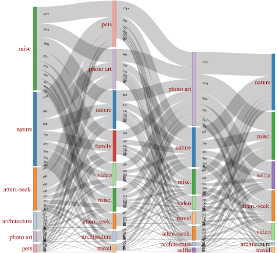
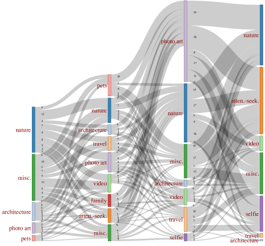
We further analyzed the evolution of topic interests over time. In this regard, we hypothesized that lurkers might exhibit patterns of topical interests that do not significantly differ from those of the other (active) users. Figure 9 shows two transition diagrams which offer a view of how the topical usage patterns change from one state (i.e., topic-set) to another, over the quarters of year 2013 in Instagram, for all users as well as for all top-25% lurkers. Let us first consider the topical evolution of all users (top of Fig. 9). Here we observe that the various levels (i.e., quarters of year 2013) are characterized by a core of topic-sets which, although with varying proportions, are always present over time (i.e., nature, attention-seeking, architecture, and miscellanea). Other topic-sets (e.g., pets and photo art) may correspond to temporary interests of users, as they are present only in some of the levels. Topical usage patterns of the users tend to continuously change over time. We in fact observe transitions from one topic-set state in a level to each of the other states in the next level. Note that such a high dynamicity is not surprising, which is explained by the inherent softness of topic categorization underlying the tags used for the uploaded media in Instagram and similar OSNs; in other terms, users can often adopt tags that naturally belong to more than one topic-set to annotate their media, according to the type of photo or video (e.g., a skyline photo can be equally relevant to the categories photo art, travel, attention-seeking). However, as it happens at the second level (quarter), all topic-set states can also show a moderate stability, since a fraction of users (about 20%) do not transition out of a topic-set state once they enter it.
Topical usage transitions in the graph of the top-ranked lurkers (bottom of Fig. 9) are also highly dynamic. The topic-sets per level are either the same as or a subset of those in the all-users graph, showing different relative proportions (i.e., frequency of usage) in some cases (e.g., family in the second level, attention-seeking in the fourth level). This would hence confirm our initial hypothesis that lurkers tend to show patterns of topical interests that do not significantly differ from the ones of all users. A major difference with the all-users graph however is that in some cases more transitions flow out from a topic-set state than the incoming ones, which corresponds to the behavior of lurkers as “newcomers”, i.e., lurkers that were not present in the immediately preceding snapshot graph, but could be in earlier snapshots (cf. Section 3.4). For instance, while several lurkers showing different interests at the second level end in the photo art state at the third level, a nearly equal proportion of new lurkers start from that state, then transition towards different topic-sets.
3.9 Time-aware ranking of lurkers
Our final research question (Q7) is devoted to the analysis of time-aware ranking of lurkers. We assess the presumed benefits derived from the use of our proposed time-transient and time-cumulative ranking models on the quality of lurker ranking solutions. In the following, we first present our evaluation methodology, then we discuss effectiveness results obtained by our time-aware LurkerRank methods and competing methods.
3.9.1 Data-driven evaluation
Evaluating lurking in OSNs is a hard problem to deal with, because of the lack of ground-truth data for lurker ranking. In the attempt of simulating a ground-truth evaluation, we build on top of our previous studies ASONAM ; SNAM14 . We generate a data-driven ranking (henceforth DD) for every network graph and use it to assess the proposed and competing methods. However, in contrast to the data-driven rankings defined in ASONAM ; SNAM14 , here we focus on the amount of actions and interactions users perform over a time interval. Formally, given and time interval , the data-driven ranking score assigned to at time is computed as:
| (19) |
where denotes the number of actions that performed at time to create new contents (e.g., media uploads), and denotes the number of information-consumption actions at time performed by in response to a specific post by . Given the characteristics of our selected datasets, we compute as the number of “favorite” or “like” actions by in relation to a media posted by . We observe however that, in general, an information-consumption action does not necessarily imply that the user will produce visible information such as posting a “like” or “comment” in response to another user’s post. Within this view, timestamped information-consumption actions could refer to the latent or silent interactions, i.e., the actions of reading or watching produced contents; unfortunately, it is not easy to build OSN datasets that are resource-rich in terms of latent interactions, mainly due to privacy policies and API limitations currently imposed by all main OSN services. We will leave the opportunity of evaluating the lurker ranking problem focusing on latent interactions as a future work (cf. Section 4.4).
3.9.2 Competing methods and assessment criteria
We compared our proposed methods Ts-LR and Te-LR against the early (i.e., time-unaware) LurkerRank (LR) SNAM14 ; ASONAM . Note that applying LR on interaction graphs is here assumed to be consistent with its definition: an interaction graph is a subset of the followship graph, however provided that only visible interactions are taken into account, which is indeed our evaluation setting.
As we presented in Section 2.2, our proposed time-aware LurkerRank methods are defined upon two models of temporal graph. Therefore, we carried out Ts-LR and Te-LR on different types of graphs, dubbed transient and cumulative snapshots, respectively. More precisely, we hereinafter refer to a monthly, transient snapshot as a snapshot whose timespan is 28 days (cf. Section 3.2). We also use the term monthly, cumulative snapshot to denote a snapshot covering a time window that is one month larger than the previous snapshot; moreover, the start time is fixed for all monthly, cumulative snapshots considered on a network dataset, thus the size of cumulative snapshots follows a non-decreasing function.
We also included in the evaluation the T-Rank algorithm BerberichVW05 , which is a time-aware adaptation of PageRank; as we discuss more in detail in Section 4, T-Rank was chosen as a competitor since, like our proposed methods, it also embeds notions of freshness and activity. We used the setting of the parameters in T-Rank as suggested in BerberichVW05 , using uniform values for both the types of coefficients that control the use of temporal information in the time-aware method: the four coefficients used to determine the random jump probabilities, and the six coefficients that give the transition probabilities of the random surfer. Note also that T-Rank was involved only in our transient evaluation case, since the algorithm was designed to work in transient snapshots. In this regard, we evaluated T-Rank on monthly, transient snapshots, setting the temporal window of interest to the last week of the month, and the tolerance interval to the first three weeks. This choice was made in order to give more importance to recent temporal information (w.r.t. the end-time of each target snapshot).
To evaluate the ranking performance of the various methods, we used two well-known assessment criteria in ranking tasks, namely Kendall-tau rank correlation coefficient abdi07 , and Fagin’s intersection metric FaginKS03 . Kendall-tau correlation evaluates the similarity between two rankings, expressed as sets of ordered pairs, based on the number of inversions of pairs which are needed to transform one ranking into the other:
Above, and are the two rankings to be compared, and is the symmetric difference distance between the two rankings, calculated as number of unshared pairs between the two lists. The score returned by is in the interval , where a value of means that the two rankings are identical and a value of means that one ranking is the reverse of the other. Fagin measure allows for determining how well two ranking lists are in agreement with each other, taking into account top-weightedness and partial rankings. Applied to any two top- lists , the Fagin score is defined as:
where denotes the sets of nodes from the 1st to the th position in the ranking. Therefore, is the average over the sum of the weighted overlaps based on the first nodes in both rankings; experimental results we shall present in Section 3.9.3 correspond to fixed to the 25% of the ranking lists being compared (denoted as @25%). Note that the score is in the interval , where means total agreement and means total disagreement.
3.9.3 Results
We focus our evaluation of time-aware LurkerRank methods on the Flickr and Instagram datasets. A major reason for this choice is that we wanted to evaluate our proposed methods against snapshots extracted from a social (followship) network as well as from an interaction network. The former scenario was evaluated thanks to the timestamped followship information that is only available in Flickr. For the latter scenario we used the timestamped information about favorite-markings available from Flickr, and the timestamped information about comments available from Instagram; note that this allowed us to evaluate the performance of the methods over snapshot graphs that correspond to two types of interactions, i.e., either “likes” or comments. Note also that we left FriendFeed out of consideration because it is less rich than Instagram in terms of timestamped information about comments; moreover, comments in FriendFeed concern user interactions corresponding to a relatively smaller portion of social graph than in Instagram (cf. Section 3.2).
| snapshot | @25% | |||
|---|---|---|---|---|
| (end time) | Te-LR | LR | Te-LR | LR |
| 2006-11-30 | 0.145 | 0.021 | 0.138 | 0.135 |
| 2006-12-28 | 0.148 | 0.007 | 0.142 | 0.135 |
| 2007-01-25 | 0.159 | -0.005 | 0.152 | 0.138 |
| 2007-02-22 | 0.178 | -0.017 | 0.156 | 0.135 |
| 2007-03-22 | 0.186 | -0.019 | 0.162 | 0.133 |
| 2007-04-19 | 0.186 | -0.017 | 0.161 | 0.133 |
| 2007-05-17 | 0.186 | -0.015 | 0.161 | 0.133 |
Table 3 shows performance results obtained on monthly snapshots of the Flickr followship network. Here we left Ts-LR out of consideration since cumulative snapshots make more sense than transient snapshots when followship relations are taken into account. In other terms, since the set of followships in a network grows progressively (unless unfollowing actions are permitted), it is unfair to consider transient snapshots which would ignore all the relations created before the selected time windows. From the table, we observe that Te-LR always obtains a higher correlation with DD than LR, with gains in terms of Kendall-tau ranging from to , and gains in terms of Fagin’s intersection up to . It should be noted that even though LR shows negative Kendall-tau correlation w.r.t. DD for more recent (i.e., cumulatively aggregated) snapshots, Fagin’s intersection values are not so distant from the ones obtained by Te-LR. This would indicate that Te-LR corresponds to a superior lurker-ranking model when applied to all users in the network as well as only to the most prominent ones as lurkers in the network, while the latter would be suboptimally detected by LR.
| snapshot | @25% | |||||
|---|---|---|---|---|---|---|
| (end time) | Ts-LR | LR | T-Rank | Ts-LR | LR | T-Rank |
| 2006-10-05 | 0.156 | -0.014 | -0.154 | 0.165 | 0.138 | 0.069 |
| 2006-11-02 | 0.169 | -0.023 | -0.167 | 0.174 | 0.133 | 0.068 |
| 2006-11-30 | 0.167 | -0.022 | -0.159 | 0.166 | 0.138 | 0.063 |
| 2006-12-28 | 0.155 | -0.003 | -0.147 | 0.171 | 0.133 | 0.068 |
| 2007-01-25 | 0.169 | -0.025 | -0.16 | 0.167 | 0.134 | 0.073 |
| 2007-02-22 | 0.167 | -0.018 | -0.159 | 0.178 | 0.14 | 0.066 |
| 2007-03-22 | 0.164 | 0 | -0.14 | 0.158 | 0.143 | 0.073 |
| avg. | 0.164 | -0.015 | -0.155 | 0.168 | 0.137 | 0.069 |
| snapshot | @25% | |||
|---|---|---|---|---|
| (end time) | Te-LR | LR | Te-LR | LR |
| 2006-10-05 | 0.156 | -0.014 | 0.165 | 0.138 |
| 2006-11-02 | 0.177 | -0.024 | 0.175 | 0.141 |
| 2006-11-30 | 0.179 | -0.030 | 0.173 | 0.140 |
| 2006-12-28 | 0.185 | -0.033 | 0.179 | 0.141 |
| 2007-01-25 | 0.191 | -0.046 | 0.177 | 0.141 |
| 2007-02-22 | 0.197 | -0.050 | 0.175 | 0.139 |
| 2007-03-22 | 0.200 | -0.050 | 0.176 | 0.138 |
Table 4 and Table 5 still focus on Flickr, however on a different scenario in which the ranking methods are applied over snapshots of the Flickr interaction network. Results from Table 4, which correspond to transient snapshots, show the better performance of Ts-LR against LR and T-Rank, according to both assessment criteria (with average Kendall-tau correlation of and average Fagin’s intersection of ). In particular, Ts-LR outperforms T-Rank, with an average gain of Kendall-tau of Fagin’s intersection. Also, Ts-LR achieves higher Kendall-tau correlation w.r.t. DD than LR (up to , with an average gain of ), while the difference in terms of Fagin’s intersection is smaller. While Kendall-tau values obtained by LR and T-Rank are negative, it should be noted that T-Rank also shows very low Fagin’s intersection values (always below ) while LR maintains a certain intersection with the top of DD (average Fagin’s intersection of ). Analogous conclusions can be drawn from the evaluation of Te-LR and LR over monthly, cumulative snapshots of the Flickr interaction network (Table 5). Again, a significant difference in terms of Kendall-tau correlation is observed between the performance of Te-LR and LR (average gap of , with LR always showing negative correlation w.r.t. DD), while Fagin’s intersection values of LR is relatively lower than the ones obtained by Te-LR (average gain of only in favor of Te-LR).
| snapshot | @25% | |||||
|---|---|---|---|---|---|---|
| (end time) | Ts-LR | LR | T-Rank | Ts-LR | LR | T-Rank |
| 2012-07-04 | 0.367 | 0.145 | 0.235 | 0.227 | 0.170 | 0.192 |
| 2012-08-01 | 0.120 | 0.107 | 0.179 | 0.244 | 0.221 | 0.103 |
| 2012-08-29 | 0.197 | 0.153 | 0.140 | 0.270 | 0.234 | 0.202 |
| 2012-09-26 | 0.255 | 0.211 | 0.111 | 0.246 | 0.205 | 0.120 |
| 2012-10-24 | 0.200 | 0.166 | 0.126 | 0.237 | 0.205 | 0.148 |
| 2012-11-21 | 0.254 | 0.234 | 0.137 | 0.185 | 0.154 | 0.108 |
| 2012-12-19 | 0.231 | 0.201 | 0.119 | 0.230 | 0.201 | 0.180 |
| 2013-01-16 | 0.236 | 0.211 | 0.095 | 0.257 | 0.235 | 0.126 |
| 2013-02-13 | 0.253 | 0.221 | 0.110 | 0.234 | 0.210 | 0.155 |
| 2013-03-13 | 0.203 | 0.166 | 0.179 | 0.195 | 0.180 | 0.154 |
| 2013-04-10 | 0.249 | 0.225 | 0.137 | 0.190 | 0.188 | 0.167 |
| 2013-05-08 | 0.282 | 0.253 | 0.099 | 0.249 | 0.235 | 0.144 |
| 2013-06-05 | 0.282 | 0.256 | 0.139 | 0.219 | 0.214 | 0.159 |
| 2013-07-03 | 0.247 | 0.216 | 0.136 | 0.227 | 0.211 | 0.135 |
| 2013-07-31 | 0.218 | 0.201 | 0.157 | 0.191 | 0.190 | 0.131 |
| 2013-08-28 | 0.236 | 0.207 | 0.143 | 0.201 | 0.181 | 0.165 |
| 2013-09-25 | 0.268 | 0.248 | 0.132 | 0.218 | 0.202 | 0.130 |
| 2013-10-23 | 0.209 | 0.191 | 0.103 | 0.183 | 0.173 | 0.156 |
| 2013-11-20 | 0.234 | 0.217 | 0.093 | 0.231 | 0.216 | 0.143 |
| 2013-12-18 | 0.226 | 0.211 | 0.115 | 0.229 | 0.224 | 0.126 |
| avg. | 0.238 | 0.202 | 0.134 | 0.223 | 0.203 | 0.147 |
| snapshot | @25% | |||
|---|---|---|---|---|
| (end time) | Te-LR | LR | Te-LR | LR |
| 2012-07-04 | 0.366 | 0.145 | 0.232 | 0.170 |
| 2012-08-01 | 0.235 | 0.112 | 0.232 | 0.203 |
| 2012-08-29 | 0.239 | 0.074 | 0.210 | 0.123 |
| 2012-09-26 | 0.233 | 0.090 | 0.185 | 0.116 |
| 2012-10-24 | 0.211 | 0.097 | 0.187 | 0.127 |
| 2012-11-21 | 0.203 | 0.101 | 0.180 | 0.128 |
| 2012-12-19 | 0.188 | 0.094 | 0.173 | 0.131 |
| 2013-01-16 | 0.175 | 0.092 | 0.178 | 0.146 |
| 2013-02-13 | 0.160 | 0.088 | 0.174 | 0.148 |
| 2013-03-13 | 0.148 | 0.079 | 0.166 | 0.144 |
| 2013-04-10 | 0.143 | 0.079 | 0.166 | 0.152 |
| 2013-05-08 | 0.137 | 0.078 | 0.163 | 0.155 |
| 2013-06-05 | 0.126 | 0.072 | 0.163 | 0.156 |
| 2013-07-03 | 0.123 | 0.076 | 0.163 | 0.159 |
| 2013-07-31 | 0.115 | 0.073 | 0.163 | 0.162 |
| 2013-08-28 | 0.112 | 0.077 | 0.166 | 0.166 |
| 2013-09-25 | 0.105 | 0.075 | 0.165 | 0.167 |
| 2013-10-23 | 0.098 | 0.075 | 0.171 | 0.177 |
| 2013-11-20 | 0.091 | 0.075 | 0.179 | 0.187 |
| 2013-12-18 | 0.088 | 0.079 | 0.182 | 0.191 |
Results over the Instagram monthly snapshots are reported in Table 6 and Table 7. Again, Ts-LR and Te-LR always perform better than competitors, in the corresponding evaluation scenarios. Moreover, compared to the results obtained on Flickr, the performance of LR is generally closer to that of the time-aware LurkerRank algorithms. In the transient evaluation case (Table 6), Kendall-tau correlation is positive for all methods, with Ts-LR showing higher correlation w.r.t. DD than T-Rank (average gain of ), and similar correlation values when compared to LR (average gain of ). An analogous situation can be depicted when considering Fagin’s intersection scores, with gains up to w.r.t. T-Rank and up to w.r.t. LR. Differences between Te-LR and LR are even smaller when looking at the cumulative case (Table 7), with always decreasing Kendall-tau gains which range from the of the first snapshot, to the of the last one. Fagin’s intersection values are very similar in most cases (maximum gain of ), with LR performing comparably to or better than Te-LR in the last snapshots. An explanation might be found according to a fact that we already observed in Section 3.3, that is, lurkers are more prone to perform actions like “favorites” or “likes” than to comment posts. Therefore, the “favorite/like” type of interaction would act as a better discriminant than “comment” in capturing the lurker dynamics via a time-varying graph model.
As a final remark, we observe that Te-LR has different overall behavior in Flickr and in Instagram time-evolving graphs, which corresponds to two diverse timespans, i.e., 7 months in Flickr against 20 months in Instagram. In particular, for more recent snapshots, ranking performance of Te-LR is generally increasing in Flickr and decreasing in Instagram, especially in terms of Kendall-tau. This would suggest a certain sensitivity of Te-LR to long timespans, which might negatively affect the Te-LR performance, even yielding worse results than the basic (i.e., time-unaware) LurkerRank.
4 Related Work
4.1 Lurking in social networks
Research studies in social science and human-computer interaction have scrutinized the various definitions of lurking, analyzed the motivational factors for lurking, and devised the main strategies for de-lurking. For instance, Soroka and Rafaeli SorokaR06 investigated relations between lurking and cultural capital, i.e., a member’s level of community-oriented knowledge, while lurking was conceptualized in CranefieldYH11 ; Muller12 in terms of the users’ boundary spanning and knowledge brokering activities across multiple community engagement spaces. The implications behind lurking were also analyzed from a group learning ChenC11 , peripheral participation HalfakerKT13 , and epistemological SchneiderKJ13 perspectives.
Understanding lurkers in OSNs refers to a scenario that has remained quite unexplored in computer science until recently. Fazeen et al. FazeenDG11 addressed classification of the various actors in an OSN (i.e., leaders, spammers, associates, and lurkers). However, in that work the lurking problem is treated marginally, and in fact lurking cases are left out of experimental evaluation. Similarly, Lang and Wu LangW13 analyzed various factors that influence lifetime of users, also distinguishing between active and passive lifetime. In this regard, a number of features is suggested to promote usage among members of OSNs like Twitter and Buzznet. Moreover, while examining to what extent active and passive lifetime are correlated, the authors observed that the study of passive lifetime requires to know the user’s last login date, which is however unavailable for many OSNs including Twitter. Besides our work on lurker detection and ranking SNAM14 ; ASONAM (previously discussed in Section 2.1), in ASONAM14 we started investigating how lurker behaviors change over time. In that work we provided a preliminary characterization of the lurking dynamics in terms of four out of the seven research questions that we have addressed in Section 3.
4.2 Time-aware PageRank
Given the popularity of PageRank among researchers in web searching of authoritative sources, most solutions for time-aware ranking have been developed in the past years by resorting to PageRank-style methods. Here we briefly discuss some of the most relevant studies, which share intuitions with our approach.
One of the earliest methods that leverage the temporal dimension in authority ranking is TimedPageRank YuLL04 . This is basically a weighted PageRank applied to a citation network in which the strength of every edge (citation) is weighted by an exponential decay function of the citation age. An aging-factor is also introduced to linearly penalize the scores w.r.t. the age of a publication. TimedPageRank adopts a graph model that represents a static picture of the network at a given time. By contrast, EventRank Smyth05 takes into account the sequence of events and can track changes in ranking over time. Originally developed for a (email) communication network, EventRank utilizes potential flow to model the exchange of messages in a cumulative ranking fashion. As mentioned in the Introduction, our time-aware lurker ranking methods also handles either approach (i.e., static or cumulative) to ranking.
Our proposed time-aware lurker ranking methods also share with T-Rank BerberichVW05 the idea of measuring freshness and activity aspects, for both individual users and their relations. T-Rank runs on a graph model in which nodes and edges are annotated with discrete temporal information, based on creation, deletion and modification timestamps of the items. A temporal window of interest and a tolerance interval are defined: the first represents the temporal range of interest to the user (e.g., duration of an event), while the latter represents a temporal window which surrounds the window of interest (e.g., the discussion that precedes and follows the event). The temporal aspects of network evolution are considered through the definition of freshness and activity functions. The freshness function depends on the time when a web page or link was last updated: it is maximal if a page or a hyperlink is updated with regard to the user’s temporal interest, and decreases linearly with the distance to the temporal window of interest. The activity function reflects the rate of updates of a page’s content and its incoming links, and it is simply defined as the sum of the freshness values of modification timestamps within the tolerance interval. The authors define two PageRank-based algorithms, namely T-Rank and T-Rank light. The latter takes into account freshness and activity functions only for skewing the random jump probabilities during the random walk process, while T-Rank skews both the random jump probabilities and the transitions probabilities based on the temporal functions.
However, we provide different technical solutions that better fit our task of lurker ranking; in particular, we provide a more refined notion of activity which allows for modeling the significant variations in the lurking score trends. Moreover, unlike T-Rank, we also define cumulative formulations of those aspects in order to enable a time-evolving graph model for the ranking of lurkers. In Section 3.9.3, we have presented an experimental comparison with T-Rank.
4.3 User activity and interaction dynamics
In this section we mention recent works which, while not addressing lurking problems, are somehow related to ours since they cope with some of the topics we have covered in Section 3, namely: user activity and interaction in temporal networks, time series and cluster analysis in social networks, topical evolution, newcomers, preferential attachment in directed networks, and responsiveness.
User activity can be influenced by many factors, including personal traits, communicative and social variables, attitudes, and social influence KrishnanA14 . Macropol et al. MacropolBSPY13 considered timing and activity information available for users to uncover correlations between topic-based user activity levels and changes in sentiment. Since user activity trends and behavioral patterns also depend on the structure and features of an OSN, they have often been studied in the context of specific OSNs. For instance, Arnaboldi et al. ArnaboldiCPD13 examined the dynamic processes of ego networks and personal social relationships in Twitter. Wang et al. WangGMZZ13 presented a detailed analysis of the dynamics of Quora, which integrates a question-answering system into an OSN, studying its user-topic graph, social graph and related questions graph. The relation between user activities and network structure can also determine the success or decline of an OSN, as studied in GarciaMS13 , where Garcia et al. analyzed the social resilience phenomenon in five online communities (i.e., Friendster, Livejournal, Facebook, Orkut and Myspace). Modeling engagement dynamics in social graphs is also the focus of the study by Malliaros and Vazirgiannis MalliarosV13 .
Time series analysis represents a key tool for modeling and mining temporal graphs, and has often been used to support clustering or classification tasks in OSNs. For instance, Yang et al. YangLY13 proposed a method for classifying Twitter users based on the content of their tweets. The method maps users to time series; more in detail, tweet features are modeled as time series in order to amplify latent periodicity patterns in user communications. Caravelli et al. CaravelliWSSM13 introduced a holistic dynamic clustering framework for identifying evolving groups and alliances across multiple time granularities in dynamic graphs.
Considering topic modeling of social media content in addition to the time dimension, Wagner et al. WagnerLPNS12 explored the impact of coupling content with user profile data on the development of the users’ topical expertise. Hu et al. HuSE14 defined a feature-based topic model and a social-based topic model in the context of large-scale user-generated documents available from OSN websites. In the context of online analysis of text streams, Saha and Sindhwani SahaS12 proposed to process incoming data together with recently seen documents over a short time window, with the purpose of producing evolving and emerging topic sets. Narang et al. NarangNMSD13 integrated text clustering, topic similarity detection and WordNet to discover time evolving conversations around topics in OSNs that do not have explicit discussion threads (e.g., Twitter).
Other specific aspects that we have analyzed in Section 3 concern the role of newcomers, the responsiveness dynamics, and the preferential attachment in directed OSNs. Concerning newcomers, recent attention has been paid to the impact of community diversity in the engagement of newcomers PanLG14 , the design of personalized engagement strategies LopezFB12 , and the antecedents of newcomers’ participation behavior TsaiP14 . Also, Allaho and Lee AllahoL13 found a tendency of collaboration between masters and newcomers in software development online communities. Responsiveness is central to gain useful insights into how users in an OSN interact with one another. Allaho and Lee AllahoL14 considered the increase in responsiveness for recommending experts in collaboration networks like Github.com. On et al. OnLJT13 investigated responsiveness coupled with engagingness behavior models in email networks, mainly for tasks of reply order prediction. Gao et al. GaoMC15 proposed an extended reinforced Poisson process model with time mapping process to capture the dynamics underlying retweets and eventually predict the future popularity of microblogs. The preferential attachment phenomenon has long received great attention in network science. Focusing on directed networks, we observe that some studies have investigated this concept as a growth model for both social media networks (e.g., Flickr mislove08wosn ) and collaboration networks (e.g., Wikipedia cap06 ). Moreover, Kunegis et al. KunegisBM13 performed an empirical study of preferential attachment in OSNs for which temporal information is available. They showed that most networks follow a nonlinear preferential attachment model, whose exponent depends on the type of network considered.
4.4 The challenge of latent user activities
In Section 3.9.1 we have raised an important issue in the evaluation of lurker ranking problems, which is related to the difficulty of gathering information about latent or silent interactions among users. These are typically performed via browsing, reading, or watching activities in the OSN environment.
There has been a number of relatively recent studies that have examined latent interactions. By using survey data obtained by nearly 1200 recruited users, Burke et al. BurkeML10 have studied user interactions on Facebook to understand relations between user-targeted visible actions (like those related to wall posts, comments, photo tagging, etc.), also called directed communication, and consumption actions, with loneliness and social capital bonding. They found that directed communication is associated with higher social capital bonding and lower loneliness, whereas social capital bridging and loneliness will increase with consumption. In a later work BernsteinBBK13 , the Facebook team further focused on the limitations of visible action indicators (like feedbacks and friend counts) in supporting the analysis of the size and profile of a user’s audience.
A useful tool for modeling both visible and latent activities of users is represented by clickstream data. Chatterjee et al. ChatterjeeHN03 proposed to trace user clickstream data to model all activities of users, suggesting main implications in the design of OSN websites and advertisement placement. Benevenuto et al. BenevenutoRCA12 provided an in-depth analysis of traffic and session patterns of user workloads. Their study is based on clickstream data that were collected through a Brazilian OSN-aggregator website. They examined how frequently users connect to OSN sites, how long users sessions are, how inter-request time and inter-session time data are distributed, and how the physical distance impacts on user interactions. Notably, Benevenuto et al. also discussed the opportunity of exploring clickstream data to understand silent interactions: in this regard, they found that browsing is the most dominant behavior in Orkut (above 90%), and that the number of friends interacting with a user increases by an order of magnitude compared to only considering visible activities of users.
Based on data collected from the largest OSN in China, RenRen, Jiang et al. JiangWWSHDZ13 conducted an extensive analysis on latent interactions focusing on profile visits. Latent interaction graphs were found to have properties that are different from both those of social graphs and visible interaction graphs. Latent interactions have extremely low reciprocity, despite the fact that RenRen allows its users to see who recently visited their profile. Compared to visible interactions, latent interactions are more prevalent and more evenly distributed across a user’s friends. A significant part of profile visits comes from non-friends of a user, while the majority of visitors do not browse the same profile twice. Moreover, profile popularity does not seem to be strictly correlated with the frequency of updates.
We envisage that the lessons learned from the above mentioned studies concerning latent activities of OSN users, could be helpful to enhance the understanding of lurking behaviors. In particular, involving information on latent activities extracted from profile visits and clickstream data, would pave the way to new opportunities of evaluation of lurker ranking problems. In this regard, we would like to stress again that our time-aware LurkerRank methods can equally deal with visible as well as latent information-consumption activities, and that they are suitable for new scenarios of data-driven ranking evaluation.
5 Conclusion
In this work, we advanced research on lurking in OSNs in a twofold manner. We studied the dynamics of lurking behaviors in OSNs, by performing a rigorous analysis aimed to understand how lurkers relate to other types of users and how patterns of lurking behaviors evolve over time. More in detail, we compared lurkers and inactive users as well as lurkers and newcomers, investigated preferential attachment between lurkers and active users, studied the lurkers’ responsiveness to others’ actions, performed a cluster analysis of the lurking trends over time and a topic-sensitive analysis of evolving patterns of lurking behavior. We also overcome the time-related limitation of previous formulations of lurker ranking methods. In this regard, we developed measures related to freshness and activity trend, both for individual users and for interactions between users. Such measures were used as key elements in time-aware LurkerRank methods, following either a time-static or a time-evolving graph model. Results have shown the significance of our time-aware LurkerRank methods. We have finally discussed open issues, concerning new opportunities of evaluation of lurker ranking problems based on the exploitation of user latent activities.
References
- (1) Abdi, H.: The Kendall Rank Correlation Coefficient. In: Encyclopedia of Measurement and Statistics (2007)
- (2) Allaho, M.Y., Lee, W.: Analyzing the social ties and structure of contributors in open source software community. In: Proc. Int. Conf. on Advances in Social Networks Analysis and Mining (ASONAM), pp. 56–60 (2013)
- (3) Allaho, M.Y., Lee, W.: Increasing the responsiveness of recommended expert collaborators for online open projects. In: Proc. ACM Conf. on Information and Knowledge Management (CIKM), pp. 749–758 (2014)
- (4) Arnaboldi, V., Conti, M., Passarella, A., Dunbar, R.: Dynamics of personal social relationships in online social networks: a study on twitter. In: Proc. ACM Conf. on Online Social Networks (COSN), pp. 15–26 (2013)
- (5) Bandura, A.: Social foundations of thought and action: A social cognitive theory. Englewood Cliffs, NJ, Prentice Hall (1986)
- (6) Benevenuto, F., Rodrigues, T., Cha, M., Almeida, V.: Characterizing user navigation and interactions in online social networks. Information Sciences 195, 1–24 (2012)
- (7) Berberich, K., Vazirgiannis, M., Weikum, G.: Time-Aware Authority Ranking. Internet Mathematics 2(3), 301–332 (2005)
- (8) Berlingerio, M., Coscia, M., Giannotti, F., Monreale, A., Pedreschi, D.: Evolving networks: Eras and turning points. Intelligent Data Analysis 17(1), 27–48 (2013)
- (9) Bernstein, M.S., Bakshy, E., Burke, M., Karrer, B.: Quantifying the invisible audience in social networks. In: Proc. ACM Conf. on Human Factors in Computing Systems (CHI), pp. 21–30 (2013)
- (10) Blei, D.M., Ng, A.Y., Jordan, M.I.: Latent Dirichlet Allocation. Journal of Machine Learning Research 3(4–5), 993–1022 (2003)
- (11) Budak, C., Agrawal, D., El Abbadi, A.: Structural trend analysis for online social networks. Proceedings of the VLDB Endowment 4(10), 646–656 (2011)
- (12) Burke, M., Marlow, C., Lento, T.: Feed me: motivating newcomer contribution in social network sites. In: Proc. ACM Conf. on Human Factors in Computing Systems (CHI), pp. 945–954 (2009)
- (13) Burke, M., Marlow, C., Lento, T.: Social network activity and social well-being. In: Proc. ACM Conf. on Human Factors in Computing Systems (CHI), pp. 1909–1912 (2010)
- (14) Capocci, A., Servedio, V.D.P., Colaiori, F., Buriol, L.S., Donato, D., Leonardi, S., Caldarelli, G.: Preferential attachment in the growth of social networks: The internet encyclopedia Wikipedia. Phys. Rev. E 74 (2006)
- (15) Caravelli, P., Wei, Y., Subak, D., Singh, L., Mann, J.: Understanding evolving group structures in time-varying networks. In: Proc. Int. Conf. on Advances in Social Networks Analysis and Mining (ASONAM), pp. 142–148 (2013)
- (16) Celli, F., Lascio, F.M.L.D., Magnani, M., Pacelli, B., Rossi, L.: Social Network Data and Practices: The Case of Friendfeed. In: Proc. Int. Conf. on Social Computing, Behavioral Modeling, and Prediction (SBP), pp. 346–353 (2010)
- (17) Cha, M., Mislove, A., Gummadi, K.P.: A Measurement-driven Analysis of Information Propagation in the Flickr Social Network. In: Proc. ACM Conf. on World Wide Web (WWW), pp. 721–730 (2009)
- (18) Chatterjee, P., Hoffman, D.L., Novak, T.P.: Modeling the clickstream: implications for web-based advertising efforts. Marketing Science 22(4), 520–541 (2003)
- (19) Chen, F.C., Chang, H.M.: Do lurking learners contribute less?: a knowledge co-construction perspective. In: Proc. Conf. on Communities and Technologies (C&T), pp. 169–178 (2011)
- (20) Cranefield, J., Yoong, P., Huff, S.L.: Beyond Lurking: The Invisible Follower-Feeder In An Online Community Ecosystem. In: Proc. Pacific Asia Conf. on Information Systems (PACIS), p. 50 (2011)
- (21) De Meo, P., Ferrara, E., Abel, F., Aroyo, L., Houben, G.J.: Analyzing user behavior across social sharing environments. ACM Trans. on Intelligent Systems and Technology 5(1) (2013)
- (22) Edelmann, N.: Reviewing the definitions of “lurkers” and some implications for online research. Cyberpsychology, Behavior, and Social Networking 16(9), 645–649 (2013)
- (23) Fagin, R., Kumar, R., Sivakumar, D.: Comparing Top k Lists. SIAM Journal on Discrete Mathematics 17(1), 134–160 (2003)
- (24) Fazeen, M., Dantu, R., Guturu, P.: Identification of leaders, lurkers, associates and spammers in a social network: context-dependent and context-independent approaches. Social Netw. Analys. Mining 1(3), 241–254 (2011)
- (25) Ferrara, E., Interdonato, R., Tagarelli, A.: Online popularity and topical interests through the lens of Instagram. In: Proc. ACM Conf. on Hypertext and Social Media (HT), pp. 24–34 (2014)
- (26) Gao, S., Ma, J., Chen, Z.: Modeling and predicting retweeting dynamics on microblogging platforms. In: Proc. ACM Conf. on Web Search and Web Data Mining (WSDM), pp. 107–116 (2015)
- (27) Garcia, D., Mavrodiev, P., Schweitzer, F.: Social resilience in online communities: the autopsy of friendster. In: Proc. ACM Conf. on Online Social Networks (COSN), pp. 39–50 (2013)
- (28) Gullo, F., Ponti, G., Tagarelli, A., Greco, S.: A time series representation model for accurate and fast similarity detection. Pattern Recognition 42(11), 2998–3014 (2009)
- (29) Halfaker, A., Keyes, O., Taraborelli, D.: Making peripheral participation legitimate: reader engagement experiments in Wikipedia. In: Proc. ACM Conf. on Computer Supported Cooperative Work (CSCW), pp. 849–860 (2013)
- (30) Hu, B., Song, Z., Ester, M.: Topic Modeling in Online Social Media, User Features, and Social Networks for. In: Encyclopedia of Social Network Analysis and Mining, pp. 2178–2191 (2014)
- (31) Jeong, H., Néda, Z., Barabási, A.L.: Measuring preferential attachment in evolving networks. EPL (Europhysics Letters) 61(4), 567 (2003)
- (32) Jiang, J., Wilson, C., Wang, X., Sha, W., Huang, P., Dai, Y., Zhao, B.Y.: Understanding latent interactions in online social networks. ACM Trans. on the Web 7(4), 18 (2013)
- (33) Krishnan, A., Atkin, D.: Individual differences in social networking site users: The interplay between antecedents and consequential effect on level of activity. Computers in Human Behavior 40, 111–118 (2014)
- (34) Kumar, R., Novak, J., Tomkins, A.: Structure and evolution of online social networks. In: Proc. ACM SIGKDD Int. Conf. on Knowledge Discovery and Data Mining (KDD), pp. 611–617 (2006)
- (35) Kunegis, J., Blattner, M., Moser, C.: Preferential attachment in online networks: measurement and explanations. In: Proc. ACM Web Science Conf. (WebSci), pp. 205–214 (2013)
- (36) Lang, J., Wu, S.F.: Social network user lifetime. Social Netw. Analys. Mining 3(3), 285–297 (2013)
- (37) Lehmann, J., Gonçalves, B., Ramasco, J.J., Cattuto, C.: Dynamical classes of collective attention in Twitter. In: Proc. ACM Conf. on World Wide Web (WWW), pp. 251–260 (2012)
- (38) Leskovec, J., Backstrom, L., Kleinberg, J.: Meme-tracking and the dynamics of the news cycle. In: Proc. ACM SIGKDD Int. Conf. on Knowledge Discovery and Data Mining (KDD), pp. 497–506. ACM (2009)
- (39) López, C., Farzan, R., Brusilovsky, P.: Personalized incremental users’ engagement: driving contributions one step forward. In: Proc. ACM Int. Conf. on Support Group Work (GROUP), pp. 189–198 (2012)
- (40) Macropol, K., Bogdanov, P., Singh, A.K., Petzold, L.R., Yan, X.: I act, therefore I judge: network sentiment dynamics based on user activity change. In: Proc. Int. Conf. on Advances in Social Networks Analysis and Mining (ASONAM), pp. 396–402 (2013)
- (41) Malliaros, F.D., Vazirgiannis, M.: To stay or not to stay: modeling engagement dynamics in social graphs. In: Proc. ACM Conf. on Information and Knowledge Management (CIKM), pp. 469–478 (2013)
- (42) Mislove, A., Koppula, H.S., Gummadi, P.K., Druschel, P., Bhattacharjee, B.: Growth of the Flickr Social Network. In: Proc. of the First Workshop on Online Social Networks (WOSN), pp. 25–30 (2008)
- (43) Muller, M.: Lurking as personal trait or situational disposition: lurking and contributing in enterprise social media. In: Proc. ACM Conf. on Computer Supported Cooperative Work (CSCW), pp. 253–256 (2012)
- (44) Narang, K., Nagar, S., Mehta, S., Subramaniam, L.V., Dey, K.: Discovery and Analysis of Evolving Topical Social Discussions on Unstructured Microblogs. In: Proc. European Conf. on Advances in Information Retrieval (ECIR), pp. 545–556 (2013)
- (45) Nonnecke, B., Preece, J.J.: Lurker demographics: counting the silent. In: Proc. ACM Conf. on Human Factors in Computing Systems (CHI), pp. 73–80 (2000)
- (46) O’Madadhain, J., Smyth, P.: EventRank: a framework for ranking time-varying networks. In: Proc. KDD Workshop on Link Discovery, pp. 9–16 (2005)
- (47) On, B., Lim, E., Jiang, J., Teow, L.: Engagingness and responsiveness behavior models on the enron email network and its application to email reply order prediction. In: The Influence of Technology on Social Network Analysis and Mining, pp. 227–253 (2013)
- (48) Pan, Z., Lu, Y., Gupta, S.: How heterogeneous community engage newcomers? The effect of community diversity on newcomers’ perception of inclusion: An empirical study in social media service. Computers in Human Behavior 39, 100–111 (2014)
- (49) Preece, J.J., Nonnecke, B., Andrews, D.: The top five reasons for lurking: improving community experiences for everyone. Computers in Human Behavior 20(2), 201–223 (2004)
- (50) Saha, A., Sindhwani, V.: Learning evolving and emerging topics in social media: a dynamic NMF approach with temporal regularization. In: Proc. ACM Conf. on Web Search and Web Data Mining (WSDM), pp. 693–702 (2012)
- (51) Schneider, A., von Krogh, G., Jager, P.: “What’s coming next?” Epistemic curiosity and lurking behavior in online communities. Computers in Human Behavior 29, 293–303 (2013)
- (52) Schwämmle, V., Jensen, O.N.: A simple and fast method to determine the parameters for fuzzy c-means cluster analysis. Bioinformatics 26(22), 2841–2848 (2010)
- (53) Soroka, V., Rafaeli, S.: Invisible participants: how cultural capital relates to lurking behavior. In: Proc. ACM Conf. on World Wide Web (WWW), pp. 163–172 (2006)
- (54) Sun, N., Rau, P.P.L., Ma, L.: Understanding lurkers in online communities: a literature review. Computers in Human Behavior 38, 110–117 (2014)
- (55) Tagarelli, A., Interdonato, R.: “Who’s out there?”: Identifying and Ranking Lurkers in Social Networks. In: Proc. Int. Conf. on Advances in Social Networks Analysis and Mining (ASONAM), pp. 215–222 (2013)
- (56) Tagarelli, A., Interdonato, R.: Lurking in social networks: topology-based analysis and ranking methods. Social Netw. Analys. Mining 4(230), 27 (2014)
- (57) Tagarelli, A., Interdonato, R.: Understanding lurking behaviors in social networks across time. In: Proc. Int. Conf. on Advances in Social Networks Analysis and Mining (ASONAM), pp. 51–55 (2014)
- (58) Tsai, H., Pai, P.: Why do newcomers participate in virtual communities? An integration of self-determination and relationship management theories. Decision Support Systems 57, 178–187 (2014)
- (59) Wagner, C., Liao, V., Pirolli, P., Nelson, L., Strohmaier, M.: It’s Not in Their Tweets: Modeling Topical Expertise of Twitter Users. In: Proc. Int. Conf. on Social Computing (SocialCom), pp. 91–100 (2012)
- (60) Wang, G., Gill, K., Mohanlal, M., Zheng, H., Zhao, B.Y.: Wisdom in the social crowd: an analysis of Quora. In: Proc. ACM Conf. on World Wide Web (WWW), pp. 1341–1352 (2013)
- (61) Wilson, C., Sala, A., Puttaswamy, K.P.N., Zhao, B.Y.: Beyond Social Graphs: User Interactions in Online Social Networks and their Implications. ACM Trans. on the Web 6(4), 17 (2012)
- (62) Yang, T., Lee, D., Yan, S.: Steeler nation, 12th man, and boo birds: classifying Twitter user interests using time series. In: Proc. Int. Conf. on Advances in Social Networks Analysis and Mining (ASONAM), pp. 684–691 (2013)
- (63) Yu, P.S., Li, X., Liu, B.: On the temporal dimension of search. In: Proc. ACM Conf. on World Wide Web (WWW), pp. 448–449 (2004)