The Approximate Capacity
of the MIMO Relay Channel

Abstract

Capacity bounds are studied for the multiple-antenna complex Gaussian relay channel with $t_{1}$ transmitting antennas at the sender, $r_{2}$ receiving and $t_{2}$ transmitting antennas at the relay, and $r_{3}$ receiving antennas at the receiver. It is shown that the partial decode–forward coding scheme achieves within $\min(t_{1},r_{2})$ bits from the cutset bound and at least one half of the cutset bound, establishing a good approximate expression of the capacity. A similar additive gap of $\min(t_{1}+t_{2},r_{3})+r_{2}$ bits is shown to be achieved by the compress–forward coding scheme.

I Introduction

The relay channel, whereby point-to-point communication between a sender and a receiver is aided by a relay, is a canonical building block for cooperative wireless communication. Introduced by van der Meulen [1], this channel model has been studied extensively in the literature, including the now classical paper by Cover and El Gamal [2]. The problem of characterizing the capacity in a computable expression, however, remains open even for simple channel models, and consequently a large body of the literature has been devoted to the study of upper and lower bounds on the capacity. Reminiscent of the max-flow min-cut theorem [3], the cutset bound was established by Cover and El Gamal [2], which sets an intuitive upper limit on the capacity. On the other direction, there are a myriad of coding schemes, typically referred to as “*–forward” [4], each establishing a lower bound on the capacity. Among these, the two most versatile coding schemes are partial decode–forward [2, Th. 7] and compress–forward [2, Th. 6], which are complementary to each other (providing digital-to-digital and analog-to-digital relays, respectively) and have been successfully extended to general relay networks for unicast, multicast, broadcast, and multiple access [5, 6, 7, 8].

The Gaussian relay channel, whereby the signals from the sender and the relay are corrupted by additive white Gaussian noise, is one of the most basic channel models studied in the literature. The capacity of the Gaussian relay channel, however, is again unknown for any nondegenerate channel parameter. Instead, the following results have been established for single-antenna Gaussian relay channels.

• Partial decode–forward and compress–forward, respectively, achieve within one bit from the cutset bound [9, 10].

• Partial decode–forward, which is a superposition of decode–forward and direct transmission, reduces to the better of the two [11].

These results establish simple approximate expressions of the capacity, which are particularly useful in high signal-to-noise ratio (SNR). A natural question arises on how these results can be extended to multiple-antenna (also known as multiple-input multiple-output or MIMO) Gaussian relay channels.

Capacity bounds for MIMO relay channels have been studied in several papers. By convex optimization techniques [12], Wang, Zhang, and Høst-Madsen [13] derived upper and lower bounds based on looser versions of the cutset bound and the decode–forward bound. These results have been improved by more advanced coding schemes (partial decode–forward and compress–forward) with suboptimal decoding rules by Simoens, Munoz-Medina, Vidal, and del Coso [14] and Ng and Foschini [15]. The usual focus of this line of work, however, has been on the optimization of resources (power and bandwidth) for practical implementations and on numerical computation of resulting capacity bounds (see also [16]). The most relevant to our main question is a recent result by Kolte, Özgür, and El Gamal [17] on a general MIMO relay network, which carefully compares the noisy network coding lower bound for the general unicast relay network [7] with the cutset bound, which can be readily specialized to the 3-node relay channel. In the same vein, another recent study by Gerdes, Hellings, Weiland, and Utschick [18] establishes the optimal input distribution of the partial decode–forward lower bound for the MIMO relay channel, the corresponding result of which for the single-antenna case is immediate since partial decode–forward is the better of decode–forward and direct transmission.

This paper provides more direct and comprehensive answers to our main question through an elementary yet careful analysis of the partial decode–forward and compress–forward lower bounds for the MIMO relay channel. The main contributions are summarized as follows.

• For the complex Gaussian relay channel with $t_{1}$ transmitting antennas at the sender, $r_{2}$ receiving and $t_{2}$ transmitting antennas at the relay, and $r_{3}$ receiving antennas at the receiver, we show that the partial decode–forward achieves within $\min(t_{1},r_{2})$ bits of the cutset bound (Theorem 1).

• This gap is somewhat relaxed when noncoherent transmission is employed (Proposition 4).

• Unlike the single-antenna counterpart, partial decode–forward can achieve rates arbitrarily higher than the better of decode–forward and direct transmission in MIMO relay channels (Proposition 5).

• To complement the additive gap result, we show that both coherent and noncoherent partial decode–forward coding schemes achieve at least half the cutset bound (Theorem 2).

• We show that compress–forward achieves $\min(t_{1}+t_{2},r_{3})+r_{2}$ bits within the cutset bound (Theorem 3).

• We establish similar results for half-duplex relay channel models [11], [19], [20] (Section VI).

In conclusion, the paper establishes simple approximate expressions of the capacity, which are particularly useful in high and low SNR. Beyond these analytical results, we also discuss how these expressions can be computed efficiently.

The rest of the paper is organized as follows. In the next section, we formally define the channel model and review the cutset upper bound, the partial decode–forward lower bound, and the compress–forward lower bound on the capacity. The main results on additive and multiplicative gaps for partial decode–forward and compress–forward are also stated therein. The proofs of these results are given in Sections III and IV. Section V is devoted to the computational aspects of our results, namely, how the capacity bounds can be computed efficiently via appropriate convex optimization formulations. Using these computational tools, the main results are verified by numerical simulations. In Section VI, half-duplex MIMO relay channels are discussed.

Throughout the paper, we use the following notation. The superscript $(\cdot)^{\scalebox{0.9}{\scriptsize${}\mathsf{H}$}}$ denotes the complex conjugate transpose of a (complex) matrix; $\mathop{\rm tr}\nolimits(\cdot)$ denotes the trace of a matrix; $I_{n}$ denotes the $n\times n$ identity matrix; $\mathbb{C}^{n\times m}$ denotes a set of $n\times m$ complex matrices; $A\succeq B$ denotes that $A-B$ is hermitian and positive semidefinite; $\operatorname{\textsf{E}}(\cdot)$ denotes the expectation with respect to the random variables in the argument.

II Problem Setup and Main Results

We model the point-to-point communication system with a relay as a MIMO relay channel with sender node 1, relay node 2, and receiver node 3; see Fig. 1. Throughout the paper, we assume the complex signal model, but corresponding results for the real case can be easily obtained; see the conference version [21] of the current paper for some results on the real model. The relay and the receiver have $r_{2}$ and $r_{3}$ receiving antennas with respective channel outputs

$$\begin{split}{\bf Y}_{2}&=G_{21}{\bf X}_{1}+{\bf Z}_{2},\\ {\bf Y}_{3}&=G_{31}{\bf X}_{1}+G_{32}{\bf X}_{2}+{\bf Z}_{3},\end{split}$$ (1)

where $G_{21}\in{\mathbb{C}^{r_{2}\times t_{1}}}$, $G_{31}\in{\mathbb{C}^{r_{3}\times t_{1}}}$, and $G_{32}\in{\mathbb{C}^{r_{3}\times t_{2}}}$ are complex channel gain matrices, and ${\bf Z}_{2}\sim\mathrm{CN}(0,I_{r_{2}})$ and ${\bf Z}_{3}\sim{\mathrm{CN}}(0,I_{r_{3}})$ are independent complex Gaussian noise components. For simplicity, we will often use the shorthand notation

$$G_{3*}=\begin{bmatrix}G_{31}&G_{32}\end{bmatrix}\quad\text{and}\quad G_{*1}=\begin{bmatrix}G_{21}\\ G_{31}\end{bmatrix}.$$

We assume that the sender and the relay have $t_{1}$ and $t_{2}$ transmitting antennas, respectively, with average power constraint $P$. As in the standard relay channel model [2], the encoder is defined by ${\bf x}_{1}^{n}(m)$, the relay encoder is defined by ${\bf x}_{2i}({\bf y}_{2}^{i-1})$, $i=1,\ldots,n$, and the decoder is defined by ${\hat{m}}({\bf y}_{3}^{n})$. We assume that the message $M$ is uniformly distributed over the message set. The average probability of error is defined as $P_{e}^{(n)}=P\{ ̂\hat{M}\neq M\}$. A rate $R$ is said to be achievable for the relay channel if there exists a sequence of $(2^{nR},n)$ codes such that $\lim_{n\to\infty}P_{e}^{(n)}=0$. The capacity $C$ of the relay channel is the supremum of all achievable rates.

\psfrag{x}[r]{${\bf X}_{1}$}\psfrag{a}[b]{$G_{21}$}\psfrag{z1}[b]{${\bf Z}_{2}$}\psfrag{y1}[l]{${\bf Y}_{\!2}$}\psfrag{x1}[r]{$\mathchar 58\relax{\bf X}_{2}$\!}\psfrag{b}[b]{$G_{32}$}\psfrag{z}[b]{${\bf Z}_{3}$}\psfrag{y}[l]{${\bf Y}_{3}$}\psfrag{1}[t]{$G_{31}$}\includegraphics[scale={0.42}]{relay-gaussian.eps}

Figure 1: The MIMO relay channel.

The following upper bound on the capacity is well known.

Proposition 1 (Cutset bound [2, Th. 4]).

The capacity $C$ of the MIMO relay channel is upper bounded by

$$R_{\mathrm{CS}} =\sup_{F({\bf x}_{1},{\bf x}_{2})}\min\bigl{\{}I({\bf X}_{1},{\bf X}_{2};{\bf Y}_{3}),$$

$$\hphantom{\;\mathrel{=}\sup_{F({\bf x}_{1},{\bf x}_{2})}\min\bigl{\{}}I({\bf X}_{1};{\bf Y}_{2},{\bf Y}_{3}\mathchoice{\mspace{1.0mu}|\mspace{1.0mu}}{|}{|}{|}{\bf X}_{2})\bigr{\}}$$ (2)

$$=\max_{K}\min\bigl{\{}{}\log\mathchoice{\mspace{1.0mu}|\mspace{1.0mu}}{|}{|}{|}I_{r_{3}}+G_{3*}KG_{3*}^{\scalebox{0.9}{\scriptsize${}\mathsf{H}$}}\mathchoice{\mspace{1.0mu}|\mspace{1.0mu}}{|}{|}{|},$$

$$\hphantom{\;\mathrel{=}\max_{K}\min\bigl{\{}}\log\mathchoice{\mspace{1.0mu}|\mspace{1.0mu}}{|}{|}{|}I_{r_{2}+r_{3}}+G_{*1}K_{1\mathchoice{\mspace{1.0mu}|\mspace{1.0mu}}{|}{|}{|}2}G_{*1}^{\scalebox{0.9}{\scriptsize${}\mathsf{H}$}}\mathchoice{\mspace{1.0mu}|\mspace{1.0mu}}{|}{|}{|}\bigr{\}}$$ (3)

$$=\max_{K}\min\bigl{\{}{}\log\mathchoice{\mspace{1.0mu}|\mspace{1.0mu}}{|}{|}{|}I_{r_{2}}+[G_{31}~{}G_{32}]K[G_{31}~{}G_{32}]^{\scalebox{0.9}{\scriptsize${}\mathsf{H}$}}\mathchoice{\mspace{1.0mu}|\mspace{1.0mu}}{|}{|}{|},$$

$$\hphantom{\;\mathrel{=}\max_{K}\min\bigl{\{}}\log\mathchoice{\mspace{1.0mu}|\mspace{1.0mu}}{|}{|}{|}I_{t_{1}}+(G_{21}^{\scalebox{0.9}{\scriptsize${}\mathsf{H}$}}G_{21}+G_{31}^{\scalebox{0.9}{\scriptsize${}\mathsf{H}$}}G_{31})K_{1\mathchoice{\mspace{1.0mu}|\mspace{1.0mu}}{|}{|}{|}2}\mathchoice{\mspace{1.0mu}|\mspace{1.0mu}}{|}{|}{|}\bigr{\}}$$ (4)

where the supremum in (2) is over all joint distributions $F({\bf x}_{1},{\bf x}_{2})$ such that $\operatorname{\textsf{E}}({\bf X}_{j}^{\scalebox{0.9}{\scriptsize${}\mathsf{H}$}}{\bf X}_{j})\leq P$, $j=1,2$, the maxima in (3) and (4) are over all $(t_{1}+t_{2})\times(t_{1}+t_{2})$ matrices

$$K=\begin{bmatrix}K_{1}&K_{12}\\ K_{12}^{\scalebox{0.9}{\scriptsize${}\mathsf{H}$}}&K_{2}\end{bmatrix}\succeq 0$$ (5)

such that $\mathop{\rm tr}\nolimits(K_{j})\leq P$, $j=1,2$, and

$$K_{1\mathchoice{\mspace{1.0mu}|\mspace{1.0mu}}{|}{|}{|}2}=K_{1}-K_{12}K_{2}^{-1}K_{12}^{\scalebox{0.9}{\scriptsize${}\mathsf{H}$}}.$$

The equality in (4) is justified by the following fact that will be used repeatedly throughout the paper.

Lemma 1.

For $\gamma\in[0,1]$, $r\times t$ matrix $G$, and $t\times t$ matrix $K\succeq 0$,

$$\mathchoice{\mspace{1.0mu}|\mspace{1.0mu}}{|}{|}{|}I_{r}+\gamma GKG^{\scalebox{0.9}{\scriptsize${}\mathsf{H}$}}\mathchoice{\mspace{1.0mu}|\mspace{1.0mu}}{|}{|}{|} =\mathchoice{\mspace{1.0mu}|\mspace{1.0mu}}{|}{|}{|}I_{t}+\gamma G^{\scalebox{0.9}{\scriptsize${}\mathsf{H}$}}GK\mathchoice{\mspace{1.0mu}|\mspace{1.0mu}}{|}{|}{|}$$

$$\geq\gamma^{\min(t,r)}\mathchoice{\mspace{1.0mu}|\mspace{1.0mu}}{|}{|}{|}I_{r}+GKG^{\scalebox{0.9}{\scriptsize${}\mathsf{H}$}}\mathchoice{\mspace{1.0mu}|\mspace{1.0mu}}{|}{|}{|}.$$ (6)

We compare the cutset bound with two lower bounds on the capacity. The first lower bound is based on the partial decode–forward coding scheme, in which the relay recovers part of the message and forwards it.

Proposition 2 (Partial decode–forward bound [2, Th. 7]).

The capacity $C$ of the MIMO relay channel is lower bounded by

$$R_{\mathrm{PDF}} =\sup\min\bigl{\{}{}I({\bf X}_{1},{\bf X}_{2};{\bf Y}_{3}),$$

$$\hphantom{\;\mathrel{=}\sup\min\bigl{\{}{}}I({\bf U};{\bf Y}_{2}\mathchoice{\mspace{1.0mu}|\mspace{1.0mu}}{|}{|}{|}{\bf X}_{2})+I({\bf X}_{1};{\bf Y}_{3}\mathchoice{\mspace{1.0mu}|\mspace{1.0mu}}{|}{|}{|}{\bf X}_{2},{\bf U})\big{\}}$$ (7)

$$=\sup\min\bigl{\{}{}I({\bf X}_{1},{\bf X}_{2};{\bf Y}_{3}),$$

$$\hphantom{\;\mathrel{=}\sup\min\bigl{\{}{}}I({\bf X}_{1};{\bf U},{\bf Y}_{3}\mathchoice{\mspace{1.0mu}|\mspace{1.0mu}}{|}{|}{|}{\bf X}_{2})-I({\bf X}_{1};{\bf U}\mathchoice{\mspace{1.0mu}|\mspace{1.0mu}}{|}{|}{|}{\bf X}_{2},{\bf Y}_{2})\big{\}}$$ (8)

where the suprema are over all joint distributions $F({\bf u},{\bf x}_{1},{\bf x}_{2})$ such that $\operatorname{\textsf{E}}({\bf X}_{j}^{\scalebox{0.9}{\scriptsize${}\mathsf{H}$}}{\bf X}_{j})\leq P$, $j=1,2$.

Remark 1.

The partial decode–forward lower bound does not increase by (coded) time sharing.

The partial decode–forward lower bound can be relaxed in several directions. First, by limiting the input distribution to a more practical product form, we obtain the noncoherent partial decode–forward lower bound:

$$R_{\mathrm{NPDF}} =\sup\min\bigl{\{}{}I({\bf X}_{1},{\bf X}_{2};{\bf Y}_{3}),$$

$$\hphantom{\;\mathrel{=}\sup\min\bigl{\{}{}}I({\bf U};{\bf Y}_{2}\mathchoice{\mspace{1.0mu}|\mspace{1.0mu}}{|}{|}{|}{\bf X}_{2})+I({\bf X}_{1};{\bf Y}_{3}\mathchoice{\mspace{1.0mu}|\mspace{1.0mu}}{|}{|}{|}{\bf X}_{2},{\bf U})\big{\}}$$ (9)

$$=\sup\min\bigl{\{}{}I({\bf X}_{1},{\bf X}_{2};{\bf Y}_{3}),$$

$$\hphantom{\;\mathrel{=}\sup\min\bigl{\{}{}}I({\bf X}_{1};{\bf U},{\bf Y}_{3}\mathchoice{\mspace{1.0mu}|\mspace{1.0mu}}{|}{|}{|}{\bf X}_{2})-I({\bf X}_{1};{\bf U}\mathchoice{\mspace{1.0mu}|\mspace{1.0mu}}{|}{|}{|}{\bf X}_{2},{\bf Y}_{2})\big{\}}$$ (10)

where the suprema are over all product distributions $F({\bf u},{\bf x}_{1})F({\bf x}_{2})$ such that $\operatorname{\textsf{E}}({\bf X}_{j}^{\scalebox{0.9}{\scriptsize${}\mathsf{H}$}}{\bf X}_{j})\leq P$, $j=1,2$. Second, by setting ${\bf U}={\bf X}_{1}$, which is equivalent to having the relay recover the entire message, we obtain the decode–forward lower bound:

$$R_{\mathrm{DF}} =\sup\min\bigl{\{}I({\bf X}_{1},{\bf X}_{2};{\bf Y}_{3}),\,I({\bf X}_{1};{\bf Y}_{2}\mathchoice{\mspace{1.0mu}|\mspace{1.0mu}}{|}{|}{|}{\bf X}_{2})\big{\}}$$ (11)

$$=\max_{K}\min\bigl{\{}{}\log\mathchoice{\mspace{1.0mu}|\mspace{1.0mu}}{|}{|}{|}I_{r_{3}}+G_{3*}KG_{3*}^{\scalebox{0.9}{\scriptsize${}\mathsf{H}$}}\mathchoice{\mspace{1.0mu}|\mspace{1.0mu}}{|}{|}{|},$$

$$\hphantom{\;\mathrel{=}\max_{K}\min\bigl{\{}{}}\log\mathchoice{\mspace{1.0mu}|\mspace{1.0mu}}{|}{|}{|}I_{r_{2}}+G_{21}K_{1\mathchoice{\mspace{1.0mu}|\mspace{1.0mu}}{|}{|}{|}2}G_{21}^{\scalebox{0.9}{\scriptsize${}\mathsf{H}$}}\mathchoice{\mspace{1.0mu}|\mspace{1.0mu}}{|}{|}{|}\bigr{\}}$$ (12)

where the supremum in (11) is over all distributions $F({\bf x}_{1},{\bf x}_{2})$ such that $\operatorname{\textsf{E}}({\bf X}_{j}^{\scalebox{0.9}{\scriptsize${}\mathsf{H}$}}{\bf X}_{j})\leq P$, $j=1,2$, and the maximum in (12) is over all $(t_{1}+t_{2})\times(t_{1}+t_{2})$ matrices $K\succeq 0$ of the form (5) such that $\mathop{\rm tr}\nolimits(K_{j})\leq P$, $j=1,2$. Third, by setting ${\bf U}=\emptyset$ and ${\bf X}_{2}=0$, we obtain the direct-transmission lower bound:

$$R_{\mathrm{DT}} =\sup I({\bf X}_{1};{\bf Y}_{3})$$

$$=\max_{K_{1}}\log\mathchoice{\mspace{1.0mu}|\mspace{1.0mu}}{|}{|}{|}I_{r_{3}}+G_{31}K_{1}G_{31}^{\scalebox{0.9}{\scriptsize${}\mathsf{H}$}}\mathchoice{\mspace{1.0mu}|\mspace{1.0mu}}{|}{|}{|}$$ (13)

where the supremum is over all distributions $F({\bf x}_{1})$ such that $\operatorname{\textsf{E}}({\bf X}_{1}^{\scalebox{0.9}{\scriptsize${}\mathsf{H}$}}{\bf X}_{1})\leq P$ and the maximum is over all $t_{1}\times t_{1}$ matrices $K_{1}\succeq 0$.

Remark 2.

Since decode–forward and direct transmission schemes are two special cases of partial decode–forward, we have in general

$$R_{\mathrm{PDF}}\geq\max(R_{\mathrm{DF}},R_{\mathrm{DT}}).$$ (14)

Next, we present another important lower bound, in which the relay compresses its noisy observation instead of recovering the message.

Proposition 3 (Compress–forward bound [2, Th. 6], [11]).

The capacity $C$ of the MIMO relay channel is lower bounded by

$$R_{\mathrm{CF}} =\sup I({\bf X}_{1};\hat{{\bf Y}}_{2},{\bf Y}_{3}\mathchoice{\mspace{1.0mu}|\mspace{1.0mu}}{|}{|}{|}{\bf X}_{2})$$ (15)

where the supremum is over all conditional distributions $F({\bf x}_{1})F({\bf x}_{2})F(\hat{{\bf y}}_{2}\mathchoice{\mspace{1.0mu}|\mspace{1.0mu}}{|}{|}{|}{\bf y}_{2},{\bf x}_{2})$ such that $\operatorname{\textsf{E}}({\bf X}_{j}^{\scalebox{0.9}{\scriptsize${}\mathsf{H}$}}{\bf X}_{j})\leq P$, $j=1,2$ and

$$I({\bf X}_{2};{\bf Y}_{3})\geq I({\bf Y}_{2};\hat{{\bf Y}}_{2}\mathchoice{\mspace{1.0mu}|\mspace{1.0mu}}{|}{|}{|}{\bf X}_{2},{\bf Y}_{3}).$$

This lower bound can be expressed equivalently as

$$R_{\mathrm{CF}} =\sup\min\bigl{\{}{}I({\bf X}_{1},{\bf X}_{2};{\bf Y}_{3})-I({\bf Y}_{2};\hat{\bf Y}_{2}\mathchoice{\mspace{1.0mu}|\mspace{1.0mu}}{|}{|}{|}{\bf X}_{1},{\bf X}_{2},{\bf Y}_{3}),$$

$$\hphantom{\;\mathrel{=}\sup\min\bigl{\{}{}}I({\bf X}_{1};\hat{{\bf Y}}_{2},{\bf Y}_{3}\mathchoice{\mspace{1.0mu}|\mspace{1.0mu}}{|}{|}{|}{\bf X}_{2})\bigr{\}}$$ (16)

where the supremum is over all conditional distributions $F({\bf x}_{1})F({\bf x}_{2})F(\hat{{\bf y}}_{2}\mathchoice{\mspace{1.0mu}|\mspace{1.0mu}}{|}{|}{|}{\bf y}_{2},{\bf x}_{2})$ such that $\operatorname{\textsf{E}}({\bf X}_{j}^{\scalebox{0.9}{\scriptsize${}\mathsf{H}$}}{\bf X}_{j})\leq P$, $j=1,2$.

Remark 3.

The compress–forward lower bound before taking the supremum in (15) or (16) is not a convex function of the conditional distribution $F({\bf x}_{1})F({\bf x}_{2})F(\hat{{\bf y}}_{2}\mathchoice{\mspace{1.0mu}|\mspace{1.0mu}}{|}{|}{|}{\bf y}_{2},{\bf x}_{2})$ in general and can be potentially improved by (coded) time sharing [22, Remark 16.4].

Remark 4.

By setting $\hat{\bf Y}_{2}=\emptyset$, compress–forward reduces to direct transmission and thus $R_{\mathrm{CF}}\geq R_{\mathrm{DT}}$.

We are now ready to state the main results of the paper.

Theorem 1.

For every $G_{21},G_{31},G_{32}$, and $P$,

$$\Delta_{\mathrm{PDF}} \mathchar 58\relax=R_{\mathrm{CS}}-R_{\mathrm{PDF}}\leq\min(t_{1},r_{2}).$$ (17)

As a supplement to the additive gap result in Theorem 1, which is useful in approximating the capacity in high SNR, we establish the following multiplicative gap to provide a tighter approximation in low SNR.

Theorem 2.

For every $G_{21},G_{31},G_{32}$, and $P$,

$$\frac{R_{\mathrm{CS}}}{R_{\mathrm{PDF}}}\leq 2.$$ (18)

In other words, partial decode–forward always achieves at least half the capacity.

The above results can be relaxed by using the noncoherent partial decode–forward.

Proposition 4.

For every $G_{21},G_{31},G_{32}$, and $P$,

$$\Delta_{\mathrm{NPDF}} \mathchar 58\relax=R_{\mathrm{CS}}-R_{\mathrm{NPDF}}$$

$$\leq\max\bigl{[}\min(t_{1},r_{2}),\,\min(t_{1}+t_{2},\,r_{3})\bigr{]}$$ (19)

and

$$\frac{R_{\mathrm{CS}}}{R_{\mathrm{NPDF}}}\leq 2.$$ (20)

For the single-antenna case, the partial decode–forward lower bound can be shown [11, Sec. II] to be equal to the maximum of the decode–forward and direct–transmission lower bounds; cf. (14). For multiple antennas, however, partial decode–forward is in general much richer than decode–forward and direct transmission.

Proposition 5.

If $t_{1},t_{2},r_{2},r_{3}\geq 2$,

$$\sup_{G_{21},G_{31},G_{32},P}\bigl{[}R_{\mathrm{PDF}}-\max(R_{\mathrm{DF}},R_{\mathrm{DT}})\bigr{]}=\infty.$$

In [17, Th. 1], Kolte, Özgür, and El Gamal derived a capacity lower bound for general MIMO relay networks. When specialized to the three-node relay network and further tightened, this result yields the following channel-independent capacity approximation.

Proposition 6.

For every $G_{21},G_{31},G_{32}$, and $P$,

$$\Delta_{\mathrm{CF}}$$

$$\mathchar 58\relax=R_{\mathrm{CS}}-R_{\mathrm{CF}}$$

$$\leq\min_{\sigma^{2}}\max\biggl{[}\min(t_{1}+t_{2},\,r_{3})\log\bigg{(}1+\frac{t_{1}+t_{2}}{\min(t_{1}+t_{2},r_{3})}\bigg{)}$$

$$\hphantom{\,\leq\min_{\sigma^{2}}\max\biggl{[}}\quad+r_{2}\log(1+1/\sigma^{2}),$$

$$\hphantom{\,\leq\min_{\sigma^{2}}\max\biggl{[}}\min(t_{1},\,r_{2}+r_{3})\log(1+\sigma^{2})\biggr{]}.$$ (21)

We tighten this result further as follows.

Theorem 3.

For every $G_{21},G_{31},G_{32}$, and $P$,

$$\Delta_{\mathrm{CF}} \leq\min_{\sigma^{2}}\max\bigl{[}\min(t_{1}+t_{2},\,r_{3})+r_{2}\log(1+1/\sigma^{2}),$$

$$\hphantom{\,\leq\min_{\sigma^{2}}\max\bigl{[}}\min(t_{1},\,r_{2}+r_{3})\log(1+\sigma^{2})\bigr{]}$$ (22)

$$\leq\min(t_{1}+t_{2},\,r_{3})+r_{2}.$$ (23)

No multiplicative gap is known between the compress–forward lower bound and the cutset bound. This follows partly from the fact that the distribution that attains the suprema in (15) and (16) is rather difficult to characterize. It can be shown, however, that when restricted to Gaussian distributions, the compress–forward lower bound (even with time sharing) may have an unbounded multiplicative gap from the cutset bound. As a compromise, we state the following simple consequence of Remark 4 and the proof of Theorem 2.

Proposition 7.

For every $G_{21},G_{31},G_{32}$, and $P$,

$$\frac{R_{\mathrm{CS}}}{\max(R_{\mathrm{DF}},R_{\mathrm{CF}})}\leq 2.$$ (24)

III Partial Decode–Forward

In this section, we establish the results on partial decode–forward stated in the previous section (Theorems 1 and 2, and Propositions 4 and 5).

III-A Partial Decode–Forward (Proof of Theorem 1)

We evaluate the partial decode–forward lower bound in (7) with $({\bf X}_{1},{\bf X}_{2})\sim\mathrm{CN}(0,K)$, where $K\succeq 0$ is of the form in (5), and

$${\bf U}=G_{21}{\bf X}_{1}+{\bf Z}^{\prime}_{2},$$ (25)

where ${\bf Z}^{\prime}_{2}\sim\mathrm{CN}(0,I_{r_{2}})$ is independent of $({\bf X}_{1},{\bf X}_{2},{\bf Z}_{2},{\bf Z}_{3})$. Note that $({\bf X}_{1},{\bf X}_{2},{\bf U},{\bf Y}_{3})$ has the same distribution as $({\bf X}_{1},{\bf X}_{2},{\bf Y}_{2},{\bf Y}_{3})$. The first term of the minimum in (7) is

$$I({\bf X}_{1},{\bf X}_{2};{\bf Y}_{3})=\log\bigr{\mathchoice{\mspace{1.0mu}|\mspace{1.0mu}}{|}{|}{|}missing}I_{r_{3}}+G_{3*}KG_{3*}^{\scalebox{0.9}{\scriptsize${}\mathsf{H}$}}\bigr{\mathchoice{\mspace{1.0mu}|\mspace{1.0mu}}{|}{|}{|}missing}.$$ (26)

For the second term, since

$$\mathop{\rm Cov}\nolimits({\bf X}_{1}\mathchoice{\mspace{1.0mu}|\mspace{1.0mu}}{|}{|}{|}{\bf U},{\bf X}_{2})$$

$$=\mathop{\rm Cov}\nolimits({\bf X}_{1}\mathchoice{\mspace{1.0mu}|\mspace{1.0mu}}{|}{|}{|}{\bf Y}_{2},{\bf X}_{2})$$

$$=K_{1\mathchoice{\mspace{1.0mu}|\mspace{1.0mu}}{|}{|}{|}2}-K_{1\mathchoice{\mspace{1.0mu}|\mspace{1.0mu}}{|}{|}{|}2}G_{21}^{\scalebox{0.9}{\scriptsize${}\mathsf{H}$}}(I_{r_{2}}+G_{21}K_{1\mathchoice{\mspace{1.0mu}|\mspace{1.0mu}}{|}{|}{|}2}G_{21}^{\scalebox{0.9}{\scriptsize${}\mathsf{H}$}})^{-1}G_{21}K_{1\mathchoice{\mspace{1.0mu}|\mspace{1.0mu}}{|}{|}{|}2}$$

$$=K_{1\mathchoice{\mspace{1.0mu}|\mspace{1.0mu}}{|}{|}{|}2}\Bigl{(}I_{t_{1}}+G_{21}^{\scalebox{0.9}{\scriptsize${}\mathsf{H}$}}G_{21}K_{1\mathchoice{\mspace{1.0mu}|\mspace{1.0mu}}{|}{|}{|}2}\Bigr{)}^{-1},$$

we have

$$I({\bf U};{\bf Y}_{2}\mathchoice{\mspace{1.0mu}|\mspace{1.0mu}}{|}{|}{|}{\bf X}_{2})+I({\bf X}_{1};{\bf Y}_{3}\mathchoice{\mspace{1.0mu}|\mspace{1.0mu}}{|}{|}{|}{\bf X}_{2},{\bf U})$$

$$=\log\frac{\mathchoice{\mspace{1.0mu}|\mspace{1.0mu}}{|}{|}{|}I_{r_{3}}+G_{31}\mathop{\rm Cov}\nolimits({\bf X}_{1}\mathchoice{\mspace{1.0mu}|\mspace{1.0mu}}{|}{|}{|}{\bf U},{\bf X}_{2})G_{31}^{\scalebox{0.9}{\scriptsize${}\mathsf{H}$}}\mathchoice{\mspace{1.0mu}|\mspace{1.0mu}}{|}{|}{|}missing}{\mathchoice{\mspace{1.0mu}|\mspace{1.0mu}}{|}{|}{|}I_{r_{2}}+G_{21}\mathop{\rm Cov}\nolimits({\bf X}_{1}\mathchoice{\mspace{1.0mu}|\mspace{1.0mu}}{|}{|}{|}{\bf U},{\bf X}_{2})G_{21}^{\scalebox{0.9}{\scriptsize${}\mathsf{H}$}}\mathchoice{\mspace{1.0mu}|\mspace{1.0mu}}{|}{|}{|}missing}$$

$$\qquad+\log{\mathchoice{\mspace{1.0mu}|\mspace{1.0mu}}{|}{|}{|}I_{r_{2}}+G_{21}K_{1\mathchoice{\mspace{1.0mu}|\mspace{1.0mu}}{|}{|}{|}2}G_{21}^{\scalebox{0.9}{\scriptsize${}\mathsf{H}$}}\mathchoice{\mspace{1.0mu}|\mspace{1.0mu}}{|}{|}{|}}$$

$$=\log\mathchoice{\mspace{1.0mu}|\mspace{1.0mu}}{|}{|}{|}I_{t_{1}}+(G_{21}^{\scalebox{0.9}{\scriptsize${}\mathsf{H}$}}G_{21}+G_{31}^{\scalebox{0.9}{\scriptsize${}\mathsf{H}$}}G_{31})K_{1\mathchoice{\mspace{1.0mu}|\mspace{1.0mu}}{|}{|}{|}2}\mathchoice{\mspace{1.0mu}|\mspace{1.0mu}}{|}{|}{|}$$

$$\qquad+\log\frac{\mathchoice{\mspace{1.0mu}|\mspace{1.0mu}}{|}{|}{|}I_{t_{1}}+G_{21}^{\scalebox{0.9}{\scriptsize${}\mathsf{H}$}}G_{21}K_{1\mathchoice{\mspace{1.0mu}|\mspace{1.0mu}}{|}{|}{|}2}\mathchoice{\mspace{1.0mu}|\mspace{1.0mu}}{|}{|}{|}missing}{\mathchoice{\mspace{1.0mu}|\mspace{1.0mu}}{|}{|}{|}I_{t_{1}}+2G_{21}^{\scalebox{0.9}{\scriptsize${}\mathsf{H}$}}G_{21}K_{1\mathchoice{\mspace{1.0mu}|\mspace{1.0mu}}{|}{|}{|}2}\mathchoice{\mspace{1.0mu}|\mspace{1.0mu}}{|}{|}{|}missing}$$ (27)

$$\geq\log\mathchoice{\mspace{1.0mu}|\mspace{1.0mu}}{|}{|}{|}I_{t_{1}}+(G_{21}^{\scalebox{0.9}{\scriptsize${}\mathsf{H}$}}G_{21}+G_{31}^{\scalebox{0.9}{\scriptsize${}\mathsf{H}$}}G_{31})K_{1\mathchoice{\mspace{1.0mu}|\mspace{1.0mu}}{|}{|}{|}2}\mathchoice{\mspace{1.0mu}|\mspace{1.0mu}}{|}{|}{|}-\min(t_{1},r_{2})$$ (28)

where the last inequality follows by Lemma 1. Comparing (26) and (28) with the cutset bound in (4) completes the proof of Theorem 1.

We can prove Theorem 1 alternatively using the following result that is applicable to a more general class of relay channels and follows by setting $p(u\mathchoice{\mspace{1.0mu}|\mspace{1.0mu}}{|}{|}{|}x_{1},x_{2})=p_{Y_{2}\mathchoice{\mspace{1.0mu}|\mspace{1.0mu}}{|}{|}{|}X_{1},X_{2}}(u\mathchoice{\mspace{1.0mu}|\mspace{1.0mu}}{|}{|}{|}x_{1},x_{2})$ in the second form of the partial decode–forward lower bound in (8).

Proposition 8.

For a discrete memoryless relay channel $p(y_{2},y_{3}\mathchoice{\mspace{1.0mu}|\mspace{1.0mu}}{|}{|}{|}x_{1},x_{2})=p(y_{2}\mathchoice{\mspace{1.0mu}|\mspace{1.0mu}}{|}{|}{|}x_{1},x_{2})p(y_{3}\mathchoice{\mspace{1.0mu}|\mspace{1.0mu}}{|}{|}{|}x_{1},x_{2})$,

$$\Delta_{\mathrm{PDF}} \mathchar 58\relax=R_{\mathrm{CS}}-R_{\mathrm{PDF}}$$

$$\leq\max_{p(x_{1},x_{2})}I(X_{1};U\mathchoice{\mspace{1.0mu}|\mspace{1.0mu}}{|}{|}{|}X_{2},Y_{2})$$

where $p(u\mathchoice{\mspace{1.0mu}|\mspace{1.0mu}}{|}{|}{|}x_{1},x_{2})=p_{Y_{2}\mathchoice{\mspace{1.0mu}|\mspace{1.0mu}}{|}{|}{|}X_{1},X_{2}}(u\mathchoice{\mspace{1.0mu}|\mspace{1.0mu}}{|}{|}{|}x_{1},x_{2})$.

Now, applying Proposition 8 to the MIMO relay channel, we have

$$I({\bf X}_{1};{\bf U}\mathchoice{\mspace{1.0mu}|\mspace{1.0mu}}{|}{|}{|}{\bf X}_{2},{\bf Y}_{2})$$

$$=\log\bigl{\mathchoice{\mspace{1.0mu}|\mspace{1.0mu}}{|}{|}{|}missing}I_{r_{3}}+G_{21}\mathop{\rm Cov}\nolimits({\bf X}_{1}\mathchoice{\mspace{1.0mu}|\mspace{1.0mu}}{|}{|}{|}{\bf Y}_{2},{\bf X}_{2})G_{21}^{\scalebox{0.9}{\scriptsize${}\mathsf{H}$}}\bigr{\mathchoice{\mspace{1.0mu}|\mspace{1.0mu}}{|}{|}{|}missing}$$

$$=\log\bigl{\mathchoice{\mspace{1.0mu}|\mspace{1.0mu}}{|}{|}{|}missing}I_{t_{1}}+G_{21}^{\scalebox{0.9}{\scriptsize${}\mathsf{H}$}}G_{21}K_{1\mathchoice{\mspace{1.0mu}|\mspace{1.0mu}}{|}{|}{|}2}(I_{t_{1}}+G_{21}^{\scalebox{0.9}{\scriptsize${}\mathsf{H}$}}G_{21}K_{1\mathchoice{\mspace{1.0mu}|\mspace{1.0mu}}{|}{|}{|}2})^{-1}\bigr{\mathchoice{\mspace{1.0mu}|\mspace{1.0mu}}{|}{|}{|}missing}$$

$$=\log\frac{\mathchoice{\mspace{1.0mu}|\mspace{1.0mu}}{|}{|}{|}I_{t_{1}}+2G_{21}^{\scalebox{0.9}{\scriptsize${}\mathsf{H}$}}G_{21}K_{1\mathchoice{\mspace{1.0mu}|\mspace{1.0mu}}{|}{|}{|}2}\mathchoice{\mspace{1.0mu}|\mspace{1.0mu}}{|}{|}{|}missing}{\mathchoice{\mspace{1.0mu}|\mspace{1.0mu}}{|}{|}{|}I_{t_{1}}+G_{21}^{\scalebox{0.9}{\scriptsize${}\mathsf{H}$}}G_{21}K_{1\mathchoice{\mspace{1.0mu}|\mspace{1.0mu}}{|}{|}{|}2}\mathchoice{\mspace{1.0mu}|\mspace{1.0mu}}{|}{|}{|}missing}$$

$$\leq\min(t_{1},r_{2}).$$

III-B Noncoherent Partial Decode–Forward (Proof of the First Statement of Proposition 4)

We use the following fact.

Lemma 2.

Let $K\succeq 0$ be of the form in (5). Then, for every $G_{31}$ and $G_{32}$, we have

$$G_{31}K_{1}G_{31}^{\scalebox{0.9}{\scriptsize${}\mathsf{H}$}}+G_{32}K_{2}G_{32}^{\scalebox{0.9}{\scriptsize${}\mathsf{H}$}}\succeq G_{32}K_{12}^{\scalebox{0.9}{\scriptsize${}\mathsf{H}$}}G_{31}^{\scalebox{0.9}{\scriptsize${}\mathsf{H}$}}+G_{31}K_{12}G_{32}^{\scalebox{0.9}{\scriptsize${}\mathsf{H}$}}.$$ (29)

Proof:

Consider

$$\begin{bmatrix}G_{31}&G_{32}\end{bmatrix}\begin{bmatrix}K_{1}&-K_{12}\\ -K_{12}^{\scalebox{0.9}{\scriptsize${}\mathsf{H}$}}&K_{2}\end{bmatrix}\begin{bmatrix}G_{31}&G_{32}\end{bmatrix}^{\scalebox{0.9}{\scriptsize${}\mathsf{H}$}}\succeq 0.$$

∎

To prove Proposition 4, let $K\succeq 0$ be of the form in (5). Let ${\bf X}_{1}\sim\mathrm{CN}(0,K_{1})$ and ${\bf X}_{2}\sim\mathrm{CN}(0,K_{2})$ be independent of each other, and define ${\bf U}$ as in (25). Then, by Lemmas 1 and 2, the first term of the minimum in the noncoherent partial decode–forward lower bound in (9) is

$$I({\bf X}_{1},{\bf X}_{2};{\bf Y}_{3})$$

$$=\log\mathchoice{\mspace{1.0mu}|\mspace{1.0mu}}{|}{|}{|}I_{r_{3}}+G_{31}K_{1}G_{31}^{\scalebox{0.9}{\scriptsize${}\mathsf{H}$}}+G_{32}K_{2}G_{32}^{\scalebox{0.9}{\scriptsize${}\mathsf{H}$}}\mathchoice{\mspace{1.0mu}|\mspace{1.0mu}}{|}{|}{|}$$ (30)

$$\geq\log\Bigl{\mathchoice{\mspace{1.0mu}|\mspace{1.0mu}}{|}{|}{|}missing}I_{r_{3}}+\mbox{\small$\displaystyle\frac{1}{2}$}(G_{31}K_{1}G_{31}^{\scalebox{0.9}{\scriptsize${}\mathsf{H}$}}+G_{32}K_{2}G_{32}^{\scalebox{0.9}{\scriptsize${}\mathsf{H}$}}$$

$$\hphantom{\geq\log\Bigl{\mathchoice{\mspace{1.0mu}|\mspace{1.0mu}}{|}{|}{|}missing}I_{r_{3}}+\mbox{\small$\displaystyle\frac{1}{2}$}(G}+G_{32}K_{12}^{\scalebox{0.9}{\scriptsize${}\mathsf{H}$}}G_{31}^{\scalebox{0.9}{\scriptsize${}\mathsf{H}$}}+G_{31}K_{12}G_{32}^{\scalebox{0.9}{\scriptsize${}\mathsf{H}$}})\Bigr{\mathchoice{\mspace{1.0mu}|\mspace{1.0mu}}{|}{|}{|}missing}$$ (31)

$$\geq\log\mathchoice{\mspace{1.0mu}|\mspace{1.0mu}}{|}{|}{|}I_{r_{3}}+G_{3*}KG_{3*}^{\scalebox{0.9}{\scriptsize${}\mathsf{H}$}}\mathchoice{\mspace{1.0mu}|\mspace{1.0mu}}{|}{|}{|}-\min(t_{1}+t_{2},\,r_{3}).$$ (32)

Following steps similar to the coherent case in Section III-A, we have

$$\mathop{\rm Cov}\nolimits({\bf X}_{1}\mathchoice{\mspace{1.0mu}|\mspace{1.0mu}}{|}{|}{|}{\bf U},{\bf X}_{2}) =\mathop{\rm Cov}\nolimits({\bf X}_{1}\mathchoice{\mspace{1.0mu}|\mspace{1.0mu}}{|}{|}{|}{\bf U})$$

$$=K_{1}(I_{t_{1}}+G_{21}^{\scalebox{0.9}{\scriptsize${}\mathsf{H}$}}G_{21}K_{1})^{-1}$$

and

$$I({\bf U};{\bf Y}_{2}\mathchoice{\mspace{1.0mu}|\mspace{1.0mu}}{|}{|}{|}{\bf X}_{2})+I({\bf X}_{1};{\bf Y}_{3}\mathchoice{\mspace{1.0mu}|\mspace{1.0mu}}{|}{|}{|}{\bf X}_{2},{\bf U})$$

$$=\log\frac{\mathchoice{\mspace{1.0mu}|\mspace{1.0mu}}{|}{|}{|}I_{r_{3}}+G_{31}\mathop{\rm Cov}\nolimits({\bf X}_{1}\mathchoice{\mspace{1.0mu}|\mspace{1.0mu}}{|}{|}{|}{\bf U})G_{31}^{\scalebox{0.9}{\scriptsize${}\mathsf{H}$}}\mathchoice{\mspace{1.0mu}|\mspace{1.0mu}}{|}{|}{|}missing}{\mathchoice{\mspace{1.0mu}|\mspace{1.0mu}}{|}{|}{|}I_{r_{2}}+G_{21}\mathop{\rm Cov}\nolimits({\bf X}_{1}\mathchoice{\mspace{1.0mu}|\mspace{1.0mu}}{|}{|}{|}{\bf U})G_{21}^{\scalebox{0.9}{\scriptsize${}\mathsf{H}$}}\mathchoice{\mspace{1.0mu}|\mspace{1.0mu}}{|}{|}{|}missing}$$

$$\qquad+\log{\mathchoice{\mspace{1.0mu}|\mspace{1.0mu}}{|}{|}{|}I_{r_{2}}+G_{21}K_{1}G_{21}^{\scalebox{0.9}{\scriptsize${}\mathsf{H}$}}\mathchoice{\mspace{1.0mu}|\mspace{1.0mu}}{|}{|}{|}}$$

$$=\log\mathchoice{\mspace{1.0mu}|\mspace{1.0mu}}{|}{|}{|}I_{t_{1}}+(G_{21}^{\scalebox{0.9}{\scriptsize${}\mathsf{H}$}}G_{21}+G_{31}^{\scalebox{0.9}{\scriptsize${}\mathsf{H}$}}G_{31})K_{1}\mathchoice{\mspace{1.0mu}|\mspace{1.0mu}}{|}{|}{|}$$

$$\qquad+\log\frac{\mathchoice{\mspace{1.0mu}|\mspace{1.0mu}}{|}{|}{|}I_{r_{2}}+G_{21}K_{1}G_{21}^{\scalebox{0.9}{\scriptsize${}\mathsf{H}$}}\mathchoice{\mspace{1.0mu}|\mspace{1.0mu}}{|}{|}{|}missing}{\mathchoice{\mspace{1.0mu}|\mspace{1.0mu}}{|}{|}{|}I_{t_{1}}+2G_{21}^{\scalebox{0.9}{\scriptsize${}\mathsf{H}$}}G_{21}K_{1}\mathchoice{\mspace{1.0mu}|\mspace{1.0mu}}{|}{|}{|}missing}$$

$$\geq\log\mathchoice{\mspace{1.0mu}|\mspace{1.0mu}}{|}{|}{|}I_{t_{1}}+(G_{21}^{\scalebox{0.9}{\scriptsize${}\mathsf{H}$}}G_{21}+G_{31}^{\scalebox{0.9}{\scriptsize${}\mathsf{H}$}}G_{31})K_{1}\mathchoice{\mspace{1.0mu}|\mspace{1.0mu}}{|}{|}{|}-\min(t_{1},r_{2}).$$ (33)

Comparing (32) and (33) with the cutset bound in (4) completes the proof.

III-C Multiplicative Gap (Proofs of Theorem 2 and the Second Statement of Proposition 4)

By setting ${\bf U}=\emptyset$ or ${\bf X}_{1}$ in (9) and specializing (12) to independent $(X_{1},X_{2})$, it can be readily checked that $R_{\mathrm{NPDF}}$ and $\max(R_{\mathrm{DF}},R_{\mathrm{DT}})$ are simultaneously lower bounded by

$$\max\Bigl{\{}{}\max_{K_{1},K_{2}}\min\bigl{(}\log\mathchoice{\mspace{1.0mu}|\mspace{1.0mu}}{|}{|}{|}I_{r_{3}}+G_{31}K_{1}G_{31}^{\scalebox{0.9}{\scriptsize${}\mathsf{H}$}}+G_{32}K_{2}G_{32}^{\scalebox{0.9}{\scriptsize${}\mathsf{H}$}}\mathchoice{\mspace{1.0mu}|\mspace{1.0mu}}{|}{|}{|},$$

$$\hphantom{\max\Bigl{\{}{}\max_{K_{1},K_{2}}\min\bigl{(}}\log\mathchoice{\mspace{1.0mu}|\mspace{1.0mu}}{|}{|}{|}I_{r_{2}}+G_{21}K_{1}G_{21}^{\scalebox{0.9}{\scriptsize${}\mathsf{H}$}}\mathchoice{\mspace{1.0mu}|\mspace{1.0mu}}{|}{|}{|}\bigr{)},$$

$$\hphantom{\max\Bigl{\{}{}}\;\,\max_{K_{1}}\log\mathchoice{\mspace{1.0mu}|\mspace{1.0mu}}{|}{|}{|}I_{r_{3}}+G_{31}K_{1}G_{31}^{\scalebox{0.9}{\scriptsize${}\mathsf{H}$}}\mathchoice{\mspace{1.0mu}|\mspace{1.0mu}}{|}{|}{|}\Bigr{\}}$$

$$=\max_{K_{1},K_{2}}\min\Bigl{\{}{}\log\mathchoice{\mspace{1.0mu}|\mspace{1.0mu}}{|}{|}{|}I_{r_{3}}+G_{31}K_{1}G_{31}^{\scalebox{0.9}{\scriptsize${}\mathsf{H}$}}+G_{32}K_{2}G_{32}^{\scalebox{0.9}{\scriptsize${}\mathsf{H}$}}\mathchoice{\mspace{1.0mu}|\mspace{1.0mu}}{|}{|}{|},$$

$$\hphantom{\;\mathrel{\geq}\max_{K_{1},K_{2}}\min\Bigl{\{}{}}\max\bigr{(}\log\mathchoice{\mspace{1.0mu}|\mspace{1.0mu}}{|}{|}{|}I_{r_{2}}+G_{21}K_{1}G_{21}^{\scalebox{0.9}{\scriptsize${}\mathsf{H}$}}\mathchoice{\mspace{1.0mu}|\mspace{1.0mu}}{|}{|}{|},$$

$$\hphantom{\;\mathrel{\geq}\max_{K_{1},K_{2}}\min\Bigl{\{}{}\max\bigr{(}}\log\mathchoice{\mspace{1.0mu}|\mspace{1.0mu}}{|}{|}{|}I_{r_{3}}+G_{31}K_{1}G_{31}^{\scalebox{0.9}{\scriptsize${}\mathsf{H}$}}\mathchoice{\mspace{1.0mu}|\mspace{1.0mu}}{|}{|}{|}\bigr{)}\Bigr{\}}.$$ (34)

We further lower bound each term in (34). By (31),

$$\log\mathchoice{\mspace{1.0mu}|\mspace{1.0mu}}{|}{|}{|}I_{r_{3}}+G_{31}K_{1}G_{31}^{\scalebox{0.9}{\scriptsize${}\mathsf{H}$}}+G_{32}K_{2}G_{32}^{\scalebox{0.9}{\scriptsize${}\mathsf{H}$}}\mathchoice{\mspace{1.0mu}|\mspace{1.0mu}}{|}{|}{|}$$

$$\geq\log\Bigl{\mathchoice{\mspace{1.0mu}|\mspace{1.0mu}}{|}{|}{|}missing}I_{r_{3}}+\mbox{\small$\displaystyle\frac{1}{2}$}(G_{31}K_{1}G_{31}^{\scalebox{0.9}{\scriptsize${}\mathsf{H}$}}+G_{32}K_{2}G_{32}^{\scalebox{0.9}{\scriptsize${}\mathsf{H}$}}$$

$$\qquad\qquad\qquad+G_{32}K_{12}^{\scalebox{0.9}{\scriptsize${}\mathsf{H}$}}G_{31}^{\scalebox{0.9}{\scriptsize${}\mathsf{H}$}}+G_{31}K_{12}G_{32}^{\scalebox{0.9}{\scriptsize${}\mathsf{H}$}})\Bigr{\mathchoice{\mspace{1.0mu}|\mspace{1.0mu}}{|}{|}{|}missing}$$

$$\geq\mbox{\small$\displaystyle\frac{1}{2}$}\log\mathchoice{\mspace{1.0mu}|\mspace{1.0mu}}{|}{|}{|}I_{r_{3}}+(G_{31}K_{1}G_{31}^{\scalebox{0.9}{\scriptsize${}\mathsf{H}$}}+G_{32}K_{2}G_{32}^{\scalebox{0.9}{\scriptsize${}\mathsf{H}$}}$$

$$\qquad\qquad\qquad+G_{32}K_{12}^{\scalebox{0.9}{\scriptsize${}\mathsf{H}$}}G_{31}^{\scalebox{0.9}{\scriptsize${}\mathsf{H}$}}+G_{31}K_{12}G_{32}^{\scalebox{0.9}{\scriptsize${}\mathsf{H}$}})\mathchoice{\mspace{1.0mu}|\mspace{1.0mu}}{|}{|}{|}.$$ (35)

Similarly,

$$\max\big{\{}\log\mathchoice{\mspace{1.0mu}|\mspace{1.0mu}}{|}{|}{|}I_{t_{1}}+G_{21}^{\scalebox{0.9}{\scriptsize${}\mathsf{H}$}}G_{21}K_{1}\mathchoice{\mspace{1.0mu}|\mspace{1.0mu}}{|}{|}{|},\log\mathchoice{\mspace{1.0mu}|\mspace{1.0mu}}{|}{|}{|}I_{t_{1}}+\!G_{31}^{\scalebox{0.9}{\scriptsize${}\mathsf{H}$}}G_{31}K_{1}\mathchoice{\mspace{1.0mu}|\mspace{1.0mu}}{|}{|}{|}\big{\}}$$

$$\geq\mbox{\small$\displaystyle\frac{1}{2}$}\big{(}\log\mathchoice{\mspace{1.0mu}|\mspace{1.0mu}}{|}{|}{|}I_{t_{1}}+\!G_{21}^{\scalebox{0.9}{\scriptsize${}\mathsf{H}$}}G_{21}K_{1}\mathchoice{\mspace{1.0mu}|\mspace{1.0mu}}{|}{|}{|}+\log\mathchoice{\mspace{1.0mu}|\mspace{1.0mu}}{|}{|}{|}I_{t_{1}}+\!G_{31}^{\scalebox{0.9}{\scriptsize${}\mathsf{H}$}}G_{31}K_{1}\mathchoice{\mspace{1.0mu}|\mspace{1.0mu}}{|}{|}{|}\big{)}$$

$$\geq\mbox{\small$\displaystyle\frac{1}{2}$}\log\big{\mathchoice{\mspace{1.0mu}|\mspace{1.0mu}}{|}{|}{|}missing}I_{t_{1}}+(G_{21}^{\scalebox{0.9}{\scriptsize${}\mathsf{H}$}}G_{21}+G_{31}^{\scalebox{0.9}{\scriptsize${}\mathsf{H}$}}G_{31})K_{1}\big{\mathchoice{\mspace{1.0mu}|\mspace{1.0mu}}{|}{|}{|}missing}.$$ (36)

Comparing (35) and (36) with the cutset bound in (4) establishes that

$$R_{\mathrm{PDF}} \geq\max(R_{\mathrm{NPDF}},R_{\mathrm{DF}},R_{\mathrm{DT}})$$

$$\geq\min\{R_{\mathrm{NPDF}},\max(R_{\mathrm{DF}},R_{\mathrm{DT}})\}\geq\mbox{\small$\displaystyle\frac{1}{2}$}R_{\mathrm{CS}}.$$ (37)

III-D Decode–Forward and Direct Transmission (Proof of Proposition 5)

Consider the MIMO relay channel with $G_{31}=\text{diag}(g,1)$, $G_{21}=\text{diag}(1,g)$, $G_{32}=\text{diag}(g,g)$, $g>1$, which is equivalent to a product of two mismatched single-antenna relay channels, one with the direct channel stronger than the sender-to-relay channel and the other in the opposite direction. Set $K_{1\mathchoice{\mspace{1.0mu}|\mspace{1.0mu}}{|}{|}{|}2}=K_{1}=K_{2}=(P/2)I_{2}$ in (26) and (28), we have

$$R_{\mathrm{PDF}} \geq\min\bigg{\{}\log\big{(}1+g^{2}P\big{)}\Big{(}1+(1+g^{2})\frac{P}{2}\Big{)},$$

$$\hphantom{\,\,\geq\min\bigg{\{}}\log\Big{(}1+(1+g^{2})\frac{P}{2}\Big{)}^{2}-2\bigg{\}}$$

$$=\log\Big{(}1+(1+g^{2})\frac{P}{2}\Big{)}^{2}-2.$$ (38)

In comparison,

$$R_{\mathrm{DF}}=R_{\mathrm{DT}} =\max_{P_{1}+P_{2}\leq P}\log(1+P_{1})(1+g^{2}P_{2})$$

$$\leq\log(1+P)(1+g^{2}P).$$ (39)

Therefore, we have

$$R_{\mathrm{PDF}}-\max(R_{\mathrm{DF}},R_{\mathrm{DT}}) \geq\log\frac{\left(1+(1+g^{2})\frac{P}{2}\right)^{2}}{(1+P)(1+g^{2}P)}-2$$

which tends to infinity as $g\to\infty$. Based on this example, more examples of larger dimensions can be constructed.

IV Compress–Forward

We prove Theorem 3. Let $K\succeq 0$ be of the form in (5). Let ${\bf X}_{1}\sim\mathrm{CN}(0,K_{1})$ and ${\bf X}_{2}\sim\mathrm{CN}(0,K_{2})$ be independent of each other, and

$$\hat{\bf Y}_{2}={\bf Y}_{2}+\hat{\bf Z}_{2}$$ (40)

where $\hat{\bf Z}_{2}\sim\mathrm{CN}(0,\sigma^{2}I_{r_{2}})$ is independent of ${\bf X}_{1},$ ${\bf X}_{2},$ ${\bf Z}_{2},$ and ${\bf Z}_{3}$. Then,

$$I({\bf Y}_{2};\hat{\bf Y}_{2}\mathchoice{\mspace{1.0mu}|\mspace{1.0mu}}{|}{|}{|}{\bf X}_{1},{\bf X}_{2},{\bf Y}_{3})$$

$$=h(\hat{\bf Y}_{2}\mathchoice{\mspace{1.0mu}|\mspace{1.0mu}}{|}{|}{|}{\bf X}_{1},{\bf X}_{2},{\bf Y}_{3})-h(\hat{\bf Y}_{2}\mathchoice{\mspace{1.0mu}|\mspace{1.0mu}}{|}{|}{|}{\bf X}_{1},{\bf X}_{2},{\bf Y}_{2},{\bf Y}_{3})$$

$$=r_{2}\log(1+1/\sigma^{2})$$ (41)

and

$$I({\bf X}_{1};\hat{\bf Y}_{2},{\bf Y}_{3}\mathchoice{\mspace{1.0mu}|\mspace{1.0mu}}{|}{|}{|}{\bf X}_{2})$$

$$=\log\frac{\Biggl{\mathchoice{\mspace{1.0mu}|\mspace{1.0mu}}{|}{|}{|}missing}\begin{bmatrix}(1+\sigma^{2})I_{r_{2}}&0\\ 0&I_{r_{3}}\end{bmatrix}+G_{*1}K_{1}G_{*1}^{\scalebox{0.9}{\scriptsize${}\mathsf{H}$}}\Biggr{\mathchoice{\mspace{1.0mu}|\mspace{1.0mu}}{|}{|}{|}missing}}{\Biggl{\mathchoice{\mspace{1.0mu}|\mspace{1.0mu}}{|}{|}{|}missing}\begin{bmatrix}(1+\sigma^{2})I_{r_{2}}&0\\ 0&I_{r_{3}}\end{bmatrix}\Biggr{\mathchoice{\mspace{1.0mu}|\mspace{1.0mu}}{|}{|}{|}missing}}$$

$$=\log\Bigl{\mathchoice{\mspace{1.0mu}|\mspace{1.0mu}}{|}{|}{|}missing}I_{t_{1}}+\Bigl{(}\frac{1}{1+\sigma^{2}}G_{21}^{\scalebox{0.9}{\scriptsize${}\mathsf{H}$}}G_{21}+G_{31}^{\scalebox{0.9}{\scriptsize${}\mathsf{H}$}}G_{31}\Bigr{)}K_{1}\Bigr{\mathchoice{\mspace{1.0mu}|\mspace{1.0mu}}{|}{|}{|}missing}$$ (42)

$$\geq\log\mathchoice{\mspace{1.0mu}|\mspace{1.0mu}}{|}{|}{|}I_{t_{1}}+(G_{21}^{\scalebox{0.9}{\scriptsize${}\mathsf{H}$}}G_{21}+G_{31}^{\scalebox{0.9}{\scriptsize${}\mathsf{H}$}}G_{31})K_{1}\mathchoice{\mspace{1.0mu}|\mspace{1.0mu}}{|}{|}{|}$$

$$\qquad-\min(t_{1},r_{2}+r_{3})\log(1+\sigma^{2}).$$ (43)

The first statement of Theorem 3 is now established by substituting (32), (41), and (43) in the compress–forward lower bound in (16) and comparing it with the cutset bound in (3). Setting $\sigma^{2}=1$ in (22) yields the second statement in (23).

V Computation of the Capacity Bounds

V-A Formulations of Optimization Problems

V-A1 Cutset Bound

Computing the cutset upper bound in (3) can be formulated as the following convex optimization problem [15]:

$$\begin{split}\text{maximize~{}~{}~{}}&R_{\mathrm{CS}}\\ \text{over~{}~{}~{}}&R_{\mathrm{CS}}\geq 0,K\succeq 0,K_{1\mathchoice{\mspace{1.0mu}|\mspace{1.0mu}}{|}{|}{|}2}\succeq 0\\ \text{subject to~{}~{}~{}}&R_{\mathrm{CS}}\leq\log\bigr{\mathchoice{\mspace{1.0mu}|\mspace{1.0mu}}{|}{|}{|}missing}I_{r_{3}}+G_{3*}KG_{3*}^{\scalebox{0.9}{\scriptsize${}\mathsf{H}$}}\bigr{\mathchoice{\mspace{1.0mu}|\mspace{1.0mu}}{|}{|}{|}missing}\\ &R_{\mathrm{CS}}\leq\log\bigl{\mathchoice{\mspace{1.0mu}|\mspace{1.0mu}}{|}{|}{|}missing}I_{r_{2}+r_{3}}+G_{*1}K_{1\mathchoice{\mspace{1.0mu}|\mspace{1.0mu}}{|}{|}{|}2}G_{*1}^{\scalebox{0.9}{\scriptsize${}\mathsf{H}$}}\bigr{\mathchoice{\mspace{1.0mu}|\mspace{1.0mu}}{|}{|}{|}missing}\\ &\mathop{\rm tr}\nolimits(A_{1}^{\scalebox{0.9}{\scriptsize${}\mathsf{H}$}}KA_{1})\leq P,\mathop{\rm tr}\nolimits(A_{2}^{\scalebox{0.9}{\scriptsize${}\mathsf{H}$}}KA_{2})\leq P\\ &K-A_{1}K_{1\mathchoice{\mspace{1.0mu}|\mspace{1.0mu}}{|}{|}{|}2}A_{1}^{\scalebox{0.9}{\scriptsize${}\mathsf{H}$}}\succeq 0\end{split}$$ (44)

where

$$A_{1}=\begin{bmatrix}I_{t_{1}}\\ 0_{t_{2}\times t_{1}}\end{bmatrix}\text{~{}~{}and~{}~{}}A_{2}=\begin{bmatrix}0_{t_{1}\times t_{2}}\\ I_{t_{2}}\end{bmatrix}.$$

The optimization problem in (44) can be solved by standard convex optimization techniques or packages, e.g., [23].

V-A2 Partial Decode–Forward Lower Bound

Since direct computation of (7) or (8) is intractable, we instead consider three lower bounds on $R_{\mathrm{PDF}}$, namely, $R_{\mathrm{DF}},R_{\mathrm{DT}}$, and the special case of $R_{\mathrm{PDF}}$ evaluated by (25), and take the maximum of the three. Note that all three lower bounds can be viewed as the partial decode–forward lower bound evaluated by (25) with a more general choice of ${\bf Z}_{2}^{\prime}\sim\mathrm{CN}(0,\sigma^{2}I_{r_{2}})$, where $\sigma^{2}=\infty,0,1$, respectively. Considering more values of $\sigma^{2}$ can further improve the bound at the cost of complexity.

As for the cutset bound, both $R_{\mathrm{DF}}$ and $R_{\mathrm{DT}}$ can be computed efficiently as a convex optimization problem. The third bound, characterized by (26) and (27), is nonconvex. Thus, we evaluate the bound with the optimal solution to the convex optimization problem defined by (26) and (28). A similar approach can be taken for computation of $R_{\mathrm{NPDF}}$.

V-A3 Compress–Forward Lower Bound

We consider two convex lower bounds on $R_{\mathrm{CF}}$, namely, the special case of $R_{\mathrm{CF}}$ evaluated by (40) with $\sigma^{2}=1$, namely,

$${\max_{K_{1},K_{2}}\min\Big{\{}{}}\log\mathchoice{\mspace{1.0mu}|\mspace{1.0mu}}{|}{|}{|}I_{r_{3}}+G_{31}K_{1}G_{31}^{\scalebox{0.9}{\scriptsize${}\mathsf{H}$}}+G_{32}K_{2}G_{32}^{\scalebox{0.9}{\scriptsize${}\mathsf{H}$}}\mathchoice{\mspace{1.0mu}|\mspace{1.0mu}}{|}{|}{|}-r_{2},$$

$$\hphantom{\max_{K_{1},K_{2}}\min\Big{\{}{}}\log\Bigl{\mathchoice{\mspace{1.0mu}|\mspace{1.0mu}}{|}{|}{|}missing}I_{t_{1}}+\Bigl{(}\frac{1}{2}G_{21}^{\scalebox{0.9}{\scriptsize${}\mathsf{H}$}}G_{21}+G_{31}^{\scalebox{0.9}{\scriptsize${}\mathsf{H}$}}G_{31}\Bigr{)}K_{1}\Bigr{\mathchoice{\mspace{1.0mu}|\mspace{1.0mu}}{|}{|}{|}missing}\Big{\}}$$

and $R_{\mathrm{DT}}$ (which corresponds to $\sigma^{2}=\infty$). As in the case of partial decode–forward, considering more values of $\sigma^{2}$ can further improve the bound at the cost of complexity.

V-B Numerical Results

We consider the additive and multiplicative gaps on 2000 $2\times 2$ MIMO relay channels with random channel gains independently distributed according to $\mathrm{CN}(0,1)$. The gaps are evaluated by relaxed bounds discussed in the previous subsection. The maximum and average of the additive gaps are shown in Fig. 2 and similar multiplicative gaps are shown in Fig. 3. The simulation results are consistent with the theoretical predictions in Theorems 1, 2, and 3, and Proposition 4.

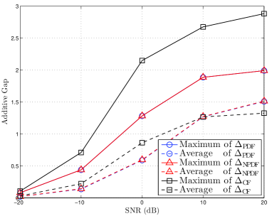
Figure 2: The additive gaps between the cutset bound and the partial decode–forward and compress–forward lower bounds for randomly generated $2\times 2$ MIMO relay channels.

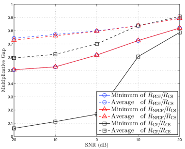
Figure 3: The multiplicative gaps between the cutset bound and the partial decode–forward and compress–forward lower bounds for randomly generated $2\times 2$ MIMO relay channels.

VI Half-Duplex MIMO Relay Channels

Half-duplex relay channel models are often investigated to study wireless communication systems in which relays cannot send and receive in the same time slot or frequency band. There are two different types of half-duplex models. One is the sender frequency-division (SFD) MIMO relay channel (Fig. 4(a)), in which the channel from the sender to the relay, ${\bf X}_{1}^{\prime\prime}\to{\bf Y}_{2}$, is orthogonal to the multiple access channel from the sender and the relay to the receiver, $({\bf X}_{1}^{\prime},{\bf X}_{2})\to{\bf Y}_{3}$. The other is the receiver frequency-division (RFD) MIMO relay channel (Fig. 4(b)), in which the channel ${\bf X}_{2}\to{\bf Y}_{3}^{\prime\prime}$ is orthogonal to the broadcast channel ${\bf X}_{1}\to({\bf Y}_{2},{\bf Y}_{3}^{\prime})$. Both can be viewed as special cases of the general (full-duplex) MIMO relay channel model. For example, the SFD model follows by setting $\begin{bmatrix}G_{31}&0\end{bmatrix}\in\mathbb{C}^{r_{3}\times(t_{1}^{\prime}+t_{1}^{\prime\prime})}$ and $\begin{bmatrix}0&G_{21}\end{bmatrix}\in\mathbb{C}^{r_{3}\times(t_{1}^{\prime}+t_{1}^{\prime\prime})}$ in (1). Consequently, our main results in Section II continue to hold with $t_{1}=t_{1}^{\prime}+t_{1}^{\prime\prime}$ and $r_{3}=r_{3}^{\prime}+r_{3}^{\prime\prime}$ for the SFD and RFD cases, respectively.

In the following, we present tighter results that exploit the half-duplex channel structure. The proofs are similar to the full-duplex case in basic analysis techniques and relegated to the Appendix.

\psfrag{xr}[r]{${\bf X}_{1}^{\prime\prime}$}\psfrag{xd}[r]{${\bf X}_{1}^{\prime}$}\psfrag{a}[b]{$G_{21}$ }\psfrag{z1}[b]{${\bf Z}_{2}$}\psfrag{y1}[l]{${\bf Y}_{\!2}$}\psfrag{x1}[r]{${\bf X}_{2}$}\psfrag{x1}[r]{$\mathchar 58\relax{\bf X}_{2}$\!}\psfrag{b}[b]{$G_{32}$}\psfrag{z}[b]{${\bf Z}_{3}$}\psfrag{y}[l]{${\bf Y}_{3}$}\psfrag{1}[t]{$G_{31}$ }\includegraphics[scale={0.45}]{model-A.eps}

(a) Sender frequency division.

\psfrag{x}[r]{${\bf X}_{1}$}\psfrag{a}[b]{$G_{21}$}\psfrag{z1}[b]{${\bf Z}_{2}$}\psfrag{y1}[l]{${\bf Y}_{\!2}$}\psfrag{x1}[r]{${\bf X}_{2}$}\psfrag{x1}[r]{$\mathchar 58\relax{\bf X}_{2}$\!}\psfrag{b}[b]{$G_{32}$}\psfrag{zs}[t]{${\bf Z}_{3}^{\prime}$}\psfrag{z'}[b]{${\bf Z}_{3}^{\prime\prime}$}\psfrag{ys}[l]{${\bf Y}_{3}^{\prime}$}\psfrag{y'}[l]{${\bf Y}_{3}^{\prime\prime}$}\psfrag{1}[t]{$G_{31}$}\includegraphics[scale={0.42}]{fd-relay.eps}

(b) Receiver frequency division.

Figure 4: Half-duplex MIMO relay channels.

VI-A Sender Frequency-Division MIMO Relay Channels

It has been shown by El Gamal and Zahedi [24] that the relay channel capacity is achieved by partial decode–forward when the sender has orthogonal components. We specialize this result to the multiple-antenna case.

Proposition 9.

The capacity of the SFD MIMO relay channel is

$$C =R_{\mathrm{CS}}=R_{\mathrm{PDF}}$$

$$=\sup_{F({\bf x}_{1}^{\prime},{\bf x}_{2})F({\bf x}^{\prime\prime}_{1})}\min\{{}I({\bf X}^{\prime}_{1},{\bf X}_{2};{\bf Y}_{3}),$$

$$\hphantom{\;\mathrel{=}\sup_{F({\bf x}_{1}^{\prime},{\bf x}_{2})F({\bf x}^{\prime\prime}_{1})}\min\{{}}I({\bf X}^{\prime\prime}_{1};{\bf Y}_{2})+I({\bf X}^{\prime}_{1};{\bf Y}_{3}\mathchoice{\mspace{1.0mu}|\mspace{1.0mu}}{|}{|}{|}{\bf X}_{2})\}$$

$$=\max_{K}\min\bigg{\{}{}\log\bigg{\mathchoice{\mspace{1.0mu}|\mspace{1.0mu}}{|}{|}{|}missing}I_{r_{3}}+G_{3*}\begin{bmatrix}K^{\prime}_{1}&K^{\prime}_{12}\\ (K^{\prime}_{12})^{\scalebox{0.9}{\scriptsize${}\mathsf{H}$}}&K_{2}\end{bmatrix}G_{3*}^{\scalebox{0.9}{\scriptsize${}\mathsf{H}$}}\bigg{\mathchoice{\mspace{1.0mu}|\mspace{1.0mu}}{|}{|}{|}missing},$$

$$\hphantom{\;\mathrel{=}\max_{K}\min\bigg{\{}{}}\log\mathchoice{\mspace{1.0mu}|\mspace{1.0mu}}{|}{|}{|}I_{r_{2}}+G_{21}K_{1}^{\prime\prime}G_{21}^{\scalebox{0.9}{\scriptsize${}\mathsf{H}$}}\mathchoice{\mspace{1.0mu}|\mspace{1.0mu}}{|}{|}{|}$$

$$\hphantom{\quad=\max_{K}\min\bigg{\{}}+\log\mathchoice{\mspace{1.0mu}|\mspace{1.0mu}}{|}{|}{|}I_{r_{3}}+G_{31}K^{\prime}_{1\mathchoice{\mspace{1.0mu}|\mspace{1.0mu}}{|}{|}{|}2}G_{31}^{\scalebox{0.9}{\scriptsize${}\mathsf{H}$}}\mathchoice{\mspace{1.0mu}|\mspace{1.0mu}}{|}{|}{|}\bigg{\}}$$ (45)

where the supremum is over all $F({\bf x}_{1}^{\prime},{\bf x}_{2})F({\bf x}^{\prime\prime}_{1})$ such that $\operatorname{\textsf{E}}(({\bf X}^{\prime}_{1})^{\scalebox{0.9}{\scriptsize${}\mathsf{H}$}}{\bf X}^{\prime}_{1})+\operatorname{\textsf{E}}(({\bf X}^{\prime\prime}_{1})^{\scalebox{0.9}{\scriptsize${}\mathsf{H}$}}{\bf X}^{\prime\prime}_{1})\leq P$ and $\operatorname{\textsf{E}}({\bf X}_{2}^{\scalebox{0.9}{\scriptsize${}\mathsf{H}$}}{\bf X}_{2})\leq P$, the maximum is over all $(t_{1}^{\prime}+t_{1}^{\prime\prime}+t_{2})\times(t_{1}^{\prime}+t_{1}^{\prime\prime}+t_{2})$ matrices

$$K=\begin{bmatrix}K^{\prime}_{1}&0&K^{\prime}_{12}\\ 0&K^{\prime\prime}_{1}&0\\ (K^{\prime}_{12})^{\scalebox{0.9}{\scriptsize${}\mathsf{H}$}}&0&K_{2}\end{bmatrix}\succeq 0$$ (46)

such that $\mathop{\rm tr}\nolimits(K^{\prime}_{1}+K^{\prime\prime}_{1})\leq P$, $\mathop{\rm tr}\nolimits(K_{2})\leq P$, and $K^{\prime}_{1\mathchoice{\mspace{1.0mu}|\mspace{1.0mu}}{|}{|}{|}2}=K^{\prime}_{1}-K^{\prime}_{12}K_{2}^{-1}(K^{\prime}_{12})^{\scalebox{0.9}{\scriptsize${}\mathsf{H}$}}$.

We can establish the following (in addition to obvious corollaries from the full-duplex results).

Proposition 10.

For every $G_{21}$, $G_{31}$, $G_{32}$, and $P$,

$$\Delta_{\mathrm{NPDF}}=C-R_{\mathrm{NPDF}} \leq\min(t^{\prime}_{1}+t_{2},\,r_{3}).$$ (47)

Proposition 11.

For every $G_{21}$, $G_{31}$, $G_{32}$, and $P$,

$$\Delta_{\mathrm{CF}}=C-R_{\mathrm{CF}} \leq\min(t^{\prime}_{1}+t_{2},\,r_{3})+r_{2}.$$ (48)

VI-B Receiver Frequency-Division MIMO Relay Channels

The capacity in this case is not known in general.

Proposition 12.

The capacity $C$ of the RFD MIMO relay channel is upper bounded by

$$R_{\mathrm{CS}} =\sup_{F({\bf x}_{1})F({\bf x}_{2})}\min\{{}I({\bf X}_{1};{\bf Y}^{\prime}_{3})+I({\bf X}_{2};{\bf Y}^{\prime\prime}_{3}),$$

$$\hphantom{\;\mathrel{=}\sup_{F({\bf x}_{1})F({\bf x}_{2})}\min\{{}}I({\bf X}_{1};{\bf Y}_{2},{\bf Y}^{\prime}_{3})\}$$

$$=\max_{K_{1}}\min\Bigl{\{}{}\log\mathchoice{\mspace{1.0mu}|\mspace{1.0mu}}{|}{|}{|}I_{r_{3}}+G_{31}K_{1}G_{31}^{\scalebox{0.9}{\scriptsize${}\mathsf{H}$}}\mathchoice{\mspace{1.0mu}|\mspace{1.0mu}}{|}{|}{|}$$

$$\hphantom{\;\mathrel{=}\max_{K_{1}}\min\Bigl{\{}{}}\qquad+\max_{K_{2}}\log\mathchoice{\mspace{1.0mu}|\mspace{1.0mu}}{|}{|}{|}I_{r_{3}}+G_{32}K_{2}G_{32}^{\scalebox{0.9}{\scriptsize${}\mathsf{H}$}}\mathchoice{\mspace{1.0mu}|\mspace{1.0mu}}{|}{|}{|},$$

$$\hphantom{\;\mathrel{=}\max_{K_{1}}\min\Bigl{\{}{}}\log\mathchoice{\mspace{1.0mu}|\mspace{1.0mu}}{|}{|}{|}I_{t_{1}}+(G_{21}^{\scalebox{0.9}{\scriptsize${}\mathsf{H}$}}G_{21}+G_{31}^{\scalebox{0.9}{\scriptsize${}\mathsf{H}$}}G_{31})K_{1}\mathchoice{\mspace{1.0mu}|\mspace{1.0mu}}{|}{|}{|}\Bigr{\}}$$ (49)

where the supremum is over all $F({\bf x}_{1})F({\bf x}_{2})$ such that $\operatorname{\textsf{E}}({\bf X}_{j}^{\scalebox{0.9}{\scriptsize${}\mathsf{H}$}}{\bf X}_{j})\leq P$, $j=1,2$, and the maxima are over all $K_{1},K_{2}\succeq 0$ such that $\mathop{\rm tr}\nolimits(K_{j})\leq P$, $j=1,2$.

As in the cutset bound, coherent transmission is irrelevant.

Proposition 13.

For every $G_{21},G_{31},G_{32}$, and $P$,

$$R_{\mathrm{PDF}}=R_{\mathrm{NPDF}}$$

and consequently

$$\Delta_{\mathrm{PDF}}=\Delta_{\mathrm{NPDF}}\leq\min(t_{1},r_{2}).$$

We can further establish the following.

Proposition 14.

For every $G_{21},G_{31},G_{32}$, and $P$,

$$\Delta_{\mathrm{CF}}\leq\max[\min(t_{1},\,r_{2}+r^{\prime}_{3}),r_{2}].$$ (50)

Proof:

Set $K^{\prime}_{12}=0$ and $K_{1\mathchoice{\mspace{1.0mu}|\mspace{1.0mu}}{|}{|}{|}2}^{\prime}=K_{1}^{\prime}$ in (9). The result follows by similar arguments to (32). ∎

Proof:

Let $K$ be the form of (46). Let ${\bf X}^{\prime}_{1}\sim\mathrm{CN}(0,K^{\prime}_{1})$, ${\bf X}^{\prime\prime}_{1}\sim\mathrm{CN}(0,K^{\prime\prime}_{1})$, and ${\bf X}_{2}\sim\mathrm{CN}(0,K_{2})$ be independent and $\hat{\bf Y}_{2}={\bf Y}_{2}+\hat{\bf Z}_{2}$, where $\hat{\bf Z}_{2}\sim\mathrm{CN}(0,I_{r_{2}})$ is independent of $({\bf X}^{\prime}_{1},{\bf X}^{\prime\prime}_{1},{\bf X}_{2},{\bf Z}_{2},{\bf Z}_{3})$. Then,

$$I({\bf X}_{1},{\bf X}_{2};{\bf Y}_{3})-I({\bf Y}_{2};\hat{{\bf Y}}_{2}\mathchoice{\mspace{1.0mu}|\mspace{1.0mu}}{|}{|}{|}{\bf X}_{1},{\bf X}_{2},{\bf Y}_{3})$$

$$\qquad=\log\mathchoice{\mspace{1.0mu}|\mspace{1.0mu}}{|}{|}{|}I_{r_{3}}+G_{31}K^{\prime}_{1}G_{31}^{\scalebox{0.9}{\scriptsize${}\mathsf{H}$}}+G_{32}K_{2}G_{32}^{\scalebox{0.9}{\scriptsize${}\mathsf{H}$}}\mathchoice{\mspace{1.0mu}|\mspace{1.0mu}}{|}{|}{|}-r_{2}$$

and

$$I({\bf X}_{1};\hat{{\bf Y}}_{2},{\bf Y}_{3}\mathchoice{\mspace{1.0mu}|\mspace{1.0mu}}{|}{|}{|}{\bf X}_{2})$$

$$=\log\mathchoice{\mspace{1.0mu}|\mspace{1.0mu}}{|}{|}{|}I_{r_{3}}+G_{31}K^{\prime}_{1}G_{31}^{\scalebox{0.9}{\scriptsize${}\mathsf{H}$}}\mathchoice{\mspace{1.0mu}|\mspace{1.0mu}}{|}{|}{|}+\log\mathchoice{\mspace{1.0mu}|\mspace{1.0mu}}{|}{|}{|}I_{r_{2}}+(1/2)G_{21}K^{\prime\prime}_{1}G_{21}^{\scalebox{0.9}{\scriptsize${}\mathsf{H}$}}\mathchoice{\mspace{1.0mu}|\mspace{1.0mu}}{|}{|}{|}$$

$$\geq\log\mathchoice{\mspace{1.0mu}|\mspace{1.0mu}}{|}{|}{|}I_{r_{3}}+G_{31}K^{\prime}_{1}G_{31}^{\scalebox{0.9}{\scriptsize${}\mathsf{H}$}}\mathchoice{\mspace{1.0mu}|\mspace{1.0mu}}{|}{|}{|}+\log\mathchoice{\mspace{1.0mu}|\mspace{1.0mu}}{|}{|}{|}I_{r_{2}}+G_{21}K^{\prime\prime}_{1}G_{21}^{\scalebox{0.9}{\scriptsize${}\mathsf{H}$}}\mathchoice{\mspace{1.0mu}|\mspace{1.0mu}}{|}{|}{|}$$

$$\qquad-\min(t_{1}^{\prime\prime},r_{2}).$$

The gap due to the first term, $\min(t_{1}^{\prime}+t_{2},r_{3})+r_{2}$, follows by similar arguments to the proof of Proposition 10, which dominates the gap due to the second term. ∎

Proof:

The compress–forward lower bound in (16) simplifies to

$$R_{\mathrm{CF}} =\sup\min\bigl{\{}{}I({\bf X}_{1};{\bf Y}^{\prime}_{3})+I({\bf X}_{2};{\bf Y}^{\prime\prime}_{3})\!-\!I({\bf Y}_{2};\hat{{\bf Y}}_{2}\mathchoice{\mspace{1.0mu}|\mspace{1.0mu}}{|}{|}{|}{\bf X}_{1}),$$

$$\hphantom{\;\mathrel{=}\sup\min\bigl{\{}{}}I({\bf X}_{1};\hat{{\bf Y}}_{2},{\bf Y}^{\prime}_{3})\bigr{\}}$$ (51)

where the supremum is over all conditional distributions $F({\bf x}_{1})F({\bf x}_{2})F(\hat{{\bf y}}_{2}\mathchoice{\mspace{1.0mu}|\mspace{1.0mu}}{|}{|}{|}{\bf y}_{2})$ such that $\operatorname{\textsf{E}}({\bf X}_{j}^{\scalebox{0.9}{\scriptsize${}\mathsf{H}$}}{\bf X}_{j})\leq P$, $j=1,2$. Let ${\bf X}_{1}\sim\mathrm{CN}(0,K_{1})$ and ${\bf X}_{2}\sim\mathrm{CN}(0,K_{2})$ be independent of each other. Let $\hat{\bf Y}_{2}={\bf Y}_{2}+\hat{\bf Z}_{2}$, where $\hat{\bf Z}_{2}\sim\mathrm{CN}(0,I_{r_{2}})$ is independent of $({\bf X}_{1},{\bf X}_{2},{\bf Z}_{2},{\bf Z}^{\prime}_{3},{\bf Z}^{\prime\prime}_{3})$. Then,

$$I({\bf X}_{1};{\bf Y}^{\prime}_{3})+I({\bf X}_{2};{\bf Y}^{\prime\prime}_{3})-I({\bf Y}_{2};\hat{{\bf Y}}_{2}\mathchoice{\mspace{1.0mu}|\mspace{1.0mu}}{|}{|}{|}{\bf X}_{1})$$

$$=\log\mathchoice{\mspace{1.0mu}|\mspace{1.0mu}}{|}{|}{|}I_{r_{3}}+G_{31}K_{1}G_{31}^{\scalebox{0.9}{\scriptsize${}\mathsf{H}$}}\mathchoice{\mspace{1.0mu}|\mspace{1.0mu}}{|}{|}{|}+\log\mathchoice{\mspace{1.0mu}|\mspace{1.0mu}}{|}{|}{|}I_{r_{3}}+G_{32}K_{2}G_{32}^{\scalebox{0.9}{\scriptsize${}\mathsf{H}$}}\mathchoice{\mspace{1.0mu}|\mspace{1.0mu}}{|}{|}{|}-r_{2}$$

and

$$I({\bf X}_{1};\hat{{\bf Y}}_{2},{\bf Y}^{\prime}_{3})=\log\Bigl{\mathchoice{\mspace{1.0mu}|\mspace{1.0mu}}{|}{|}{|}missing}I_{t_{1}}+\Bigl{(}\mbox{\small$\displaystyle\frac{1}{2}$}G_{21}^{\scalebox{0.9}{\scriptsize${}\mathsf{H}$}}G_{21}+G_{31}^{\scalebox{0.9}{\scriptsize${}\mathsf{H}$}}G_{31}\Bigr{)}K_{1}\Bigr{\mathchoice{\mspace{1.0mu}|\mspace{1.0mu}}{|}{|}{|}missing}.$$

The rest of the proof follows similar steps to that of Proposition 11. ∎

References

- [1] E. C. van der Meulen, “The discrete memoryless channel with two senders and one receiver,” in Proc. 2nd Int. Symp. Inf. Theory, Tsahkadsor, Armenian SSR, 1971, pp. 103–135.
- [2] T. M. Cover and A. El Gamal, “Capacity theorems for the relay channel,” IEEE Trans. Inf. Theory, vol. 25, no. 5, pp. 572–584, Sep. 1979.
- [3] L. R. Ford, Jr. and D. R. Fulkerson, “Maximal flow through a network,” Canad. J. Math., vol. 8, no. 3, pp. 399–404, 1956.
- [4] Y.-H. Kim, “Dictionary of relaying schemes,” 2014. [Online]. Available: http://circuit.ucsd.edu/~yhk/relaying.html
- [5] G. Kramer, M. Gastpar, and P. Gupta, “Cooperative strategies and capacity theorems for relay networks,” IEEE Trans. Inf. Theory, vol. 51, no. 9, pp. 3037–3063, Sep. 2005.
- [6] M. H. Yassaee and M. R. Aref, “Slepian-Wolf coding over cooperative relay networks,” IEEE Trans. Inf. Theory, vol. 57, no. 6, pp. 3462–3482, 2011.
- [7] S. H. Lim, Y.-H. Kim, A. El Gamal, and S.-Y. Chung, “Noisy network coding,” IEEE Trans. Inf. Theory, vol. 57, no. 5, pp. 3132–3152, May 2011.
- [8] S. H. Lim, K. T. Kim, and Y.-H. Kim, “Distributed decode–forward for relay networks,” 2015, submitted to IEEE Trans. Inf. Theory.
- [9] W. Chang, S.-Y. Chung, and Y. H. Lee, “Gaussian relay channel capacity to within a fixed number of bits,” 2010, preprint available at http://arxiv.org/abs/1011.5065/.
- [10] A. S. Avestimehr, S. N. Diggavi, and D. N. C. Tse, “Wireless network information flow: A deterministic approach,” IEEE Trans. Inf. Theory, vol. 57, no. 4, pp. 1872–1905, Apr. 2011.
- [11] A. El Gamal, M. Mohseni, and S. Zahedi, “Bounds on capacity and minimum energy-per-bit for AWGN relay channels,” IEEE Trans. Inf. Theory, vol. 52, no. 4, pp. 1545–1561, 2006.
- [12] S. Boyd and L. Vandenberghe, Convex Optimization. Cambridge: Cambridge University Press, 2004.
- [13] B. Wang, J. Zhang, and A. Høst-Madsen, “On the capacity of MIMO relay channels,” IEEE Trans. Inf. Theory, vol. 51, no. 1, pp. 29–43, Jan. 2005.
- [14] S. Simoens, O. Muñoz-Medina, J. Vidal, and A. del Coso, “On the Gaussian MIMO relay channel with full channel state information,” IEEE Trans. Signal Process., vol. 57, no. 9, pp. 3588–3599, 2009.
- [15] C. T. K. Ng and G. J. Foschini, “Transmit signal and bandwidth optimization in multiple-antenna relay channels,” IEEE Trans. Commun., vol. 59, no. 11, pp. 2987–2992, 2011.
- [16] L. Gerdes, L. Weiland, and W. Utschick, “A zero-forcing partial decode-and-forward scheme for the Gaussian MIMO relay channel,” in IEEE Int. Conf. Commun., Budapest, Hungary, Jun 2013, pp. 3349–3354.
- [17] R. Kolte, A. Özgür, and A. E. Gamal, “Capacity approximations for gaussian relay networks,” IEEE Trans. Inf. Theory, vol. 61, no. 9, pp. 4721–4734, 2015.
- [18] L. Gerdes, C. Hellings, L. Weiland, and W. Utschick, “The optimal input distribution for partial decode-and-forward in the MIMO relay channel,” CoRR, vol. abs/1409.8624, 2014. [Online]. Available: http://arxiv.org/abs/1409.8624
- [19] A. Høst-Madsen and J. Zhang, “Capacity bounds and power allocation for wireless relay channels,” IEEE Trans. Inf. Theory, vol. 51, no. 6, pp. 2020–2040, Jun. 2005.
- [20] Y. Liang and V. V. Veeravalli, “Gaussian orthogonal relay channels: Optimal resource allocation and capacity,” IEEE Trans. Inf. Theory, vol. 51, no. 9, pp. 3284–3289, Sep. 2005.
- [21] X. Jin and Y. Kim, “Approximate capacity of the MIMO relay channel,” in 2014 Proc. IEEE Int. Symp. Inf. Theory, Honolulu, HI, USA, June 29 - July 4, 2014, 2014, pp. 2102–2106.
- [22] A. El Gamal and Y.-H. Kim, Network Information Theory. Cambridge: Cambridge University Press, 2011.
- [23] M. Grant and S. Boyd, “CVX: Matlab software for disciplined convex programming, version 2.0 beta,” http://cvxr.com/cvx, Sep. 2013.
- [24] A. El Gamal and S. Zahedi, “Capacity of a class of relay channels with orthogonal components,” IEEE Trans. Inf. Theory, vol. 51, no. 5, pp. 1815–1817, 2005.