Above-threshold ionization and photoelectron spectra in atomic systems driven by strong laser fields

Abstract

Above-threshold ionization (ATI) results from strong field laser-matter interaction and it is one of the fundamental processes that may be used to extract electron structural and dynamical information about the atomic or molecular target. Moreover, it can also be used to characterize the laser field itself. Here, we develop an analytical description of ATI, which extends the theoretical Strong Field Approximation (SFA), for both the direct and re-scattering transition amplitudes in atoms. From a non-local, but separable potential, the bound-free dipole and the re-scattering transition matrix elements are analytically computed. In comparison with the standard approaches to the ATI process, our analytical derivation of the re-scattering matrix elements allows us to study directly how the re-scattering process depends on the atomic target and laser pulse features – we can turn on and off contributions having different physical origins or corresponding to different physical mechanisms. We compare SFA results with the full numerical solutions of the time-dependent Schrödinger equation (TDSE) within the few-cycle pulse regime. Good agreement between our SFA and TDSE model is found for the ATI spectrum. Our model captures also the strong dependence of the photoelectron spectra on the carrier envelope phase of the laser field.

I Introduction

During the last three decades, advances in laser technology and the understanding of nonlinear processes in laser-matter interactions have led to production of few-cycle femtosecond (1 fs $\>=10^{-15}$ s) laser pulses in the visible and mid-infrared regimes Nisoli et al. (1997); Hemmer et al. (2013). By focusing such ultrashort laser pulses on a gas target, the atoms are subjected to an ultra-intense electric field, with peak field strengths approaching the binding field inside the atoms themselves. Such fields are commonly used as a tool to explore the interaction between strong electromagnetic coherent radiation and an atomic or molecular system with unprecedented spatial and temporal resolution Krausz and Ivanov (2009). Phenomena such as high-order harmonic generation (HHG) L’Huillier and Balcou (1993); McPherson et al. (1987), above-threshold ionization Agostini et al. (1979), multi-photon ionization and multi-electron effects Mainfray and Manus (1991); Uiberacker et al. (2007), are routinely studied. These effects can be used to generate attosecond pulses in the extreme ultraviolet Drescher et al. (2001); Zhao et al. (2012) or even soft X-ray regime Silva et al. (2015). They can also be used to extract either information about the laser pulse electric field itself Paulus et al. (2001), or about the structure of the target atom or molecule Blaga et al. (2012); Pullen et al. (2015).

Since electronic motion is governed by the waveform of the laser electric field, an important quantity to describe the electric field shape is the so-called absolute phase or carrier-to-envelope-phase (CEP). Control over the CEP is paramount for extracting information about electron dynamics, and to retrieve structural information from atoms and molecules Baltuška et al. (2003); Itatani et al. (2004); Wolter et al. (2014). For instance, in HHG an electron is liberated from an atom or molecule through ionization, which occurs close to the maximum of the electric field. Within the oscillating field, the electron can thus accelerate along oscillating trajectories, which may result in re-collision with the parent ion, roughly when the laser field approaches a zero value. Control over the CEP is particularly important for HHG, when targets are driven by laser pulses comprising only one or two optical cycles. In such situation CEP determines the relevant electron trajectories, i.e. the CEP determines whether emission results in a single or in multiple attosecond bursts of radiation Baltuška et al. (2003); Sola et al. (2006).

The influence of the CEP on electron emission was also demonstrated in an anti-correlation experiment, in which the number of ATI electrons emitted in opposite directions was measured Paulus et al. (2001); Milošević et al. (2006). Since the first proof of principle experiment Paulus et al. (2001), the stereo ATI technique has established itself as a direct measure of the CEP, and demonstrated its ability for single shot measurements even at multiple kHz laser repetition rates. The sensitivity to the CEP arises from contributions of both, bound-free and the re-scattering continuum-continuum transitions of the atomic or molecular target, which are embedded in the photoelectron distribution of ATI Itatani et al. (2004). Hence, this mechanism can be used to extract structural information about the target atom or molecule.

Laser induced electron diffraction (LIED) was suggested early on as a technique that uses the doubly differential elastic scattering cross section to extract structural information  Zuo et al. (1996); Lein et al. (2002); Lin et al. (2010). Meeting the requirements to extract structural information has, however, proven difficult due to the stringent prerequisites on the laser parameters. During recent years, the development of new laser sources has dramatically advanced, leading to first demonstrations Xu et al. (2014); Meckel et al. (2008); Morishita et al. (2008); Xu et al. (2012); Pullen et al. (2015), and the successful retrieval of the bond distances in simple diatomic molecules with fixed-angle broadband electron scattering Xu et al. (2014). Recently, Pullen et al. Pullen et al. (2015) have exploited the full double differential cross section to image the entire structure of a polyatomic molecule for the first time. An important next step to exploit the full potential of the re-collision physics is the exploitation of the intrinsic time resolution of LIED to extract dynamic structural information. The key for such a goal is, however, a comprehensive and complete understanding of the ATI process and its theoretical description Milošević et al. (2006); Faisal (1973); Reiss (1980); Lewenstein et al. (1995); Frolov et al. (2014); Becker et al. (2002); Tolstikhin et al. (2010).

The aim of our paper is to revisit the strong field approximation model of M. Lewenstein for ATI for few-cycle infrared (IR) laser pulses and to compare it with the numerical solution of the TDSE in one (1D) and two (2D) spatial dimensions for an atomic system Lewenstein et al. (1995). For simplicity, our analytical atomic model is based on a non-local potential, which can be considered a short-range (SR) potential. In order to verify the validity of our analytical SR model, and to understand how its predictions compare with a true Coulomb potential, we numerically integrate the TDSE for the hydrogen atom and compute the photoelectron energy and momentum distributions.

This article is organized as follows. In Section II, we review the theory which describes the ATI process within the Strong Field Approximation; in particular, we present the derivation of the transition amplitude for both the direct and re-scattered electrons. We develop in detail the mathematical foundations towards the final results by starting from the Hamiltonian, which describes the atomic system and the TDSE associated to it. In Section III, we introduce the model for our atomic system, that uses a particular form of a non-local short-range potential. The matrix elements to describe the ionization and re-scattering processes are then computed. In section IV, the ATI spectra for the 1D line and 2D case are numerically calculated and compared with numerical results obtained from TDSE calculations. In addition, we discuss the effect of the CEP on the spectra, calculated from our analytical SFA model. Finally, in section V, we summarize the main ideas and present our conclusions. We give an outlook on extending this analytical model to more complex atomic and molecular systems.

II Strong field approximation: transition probability amplitudes

The interaction of a strong electric field with an atomic or molecular system is described within Quantum Mechanics by the time dependent Schrödinger equation that captures both the evolution of the (electronic) wave function and the time evolution of the physical observables. The numerical solution of the TDSE offers a full quantum mechanical description of the laser-matter interaction processes, and has been extensively used to study several phenomena, such as HHG Gaarde et al. (1998); Tate et al. (2007); Ciappina et al. (2012) and ATI Kulander (1987); Muller (1999); Bauer (2005); Blaga et al. (2009); Ruf et al. (2009) in atomic and molecular systems. However, the full numerical integration of the TDSE in all the degrees of freedom of the system is often a laborious, and sometimes an impossible task to perform from a numerical and computational points of view. Moreover, a physical interpretation of the numerical TDSE results and the extraction of information from the time evolved wave function is highly nontrivial for an ab initio technique.

Hence, from a purely theoretical point of view, it would be desirable to solve the TDSE analytically for the ionization process. This is one of the main steps in all laser-matter interaction phenomena, and it represents a formidable and challenging assignment. Here, we discuss an alternative method to calculate photoelectron spectra from atomic systems by analytically solving the TDSE under the so-called Strong Field Approximation. This approach dates back to Keldysh Keldysh (1965), and has since been employed by many other authors Ammosov et al. (1986); Faisal (1973); Reiss (1980); Grochmalicki et al. (1986); Ehlotzky (1992); Lewenstein et al. (1994, 1995); Kuchiev and Ostrovsky (1999). It is worth noted that SFA provides a quantum framework and extension of the, so called, “simple man’s” or “three step” or “re-collision” model, usually attributed to P. Corkum Corkum (1993), K. Kulander Krause et al. (1992); Kulander et al. (1993) and H. Muller (cf. Smirnova and Ivanov (2014) for an extensive review; for earlier quantum formulation of “Atomic Antennas” see Ref. Kuchiev (1987); for other pioneering contributions see Refs. Brunel (1987, 1990); Corkum et al. (1989)).

Ionization driven by strong fields

Let us consider an atom under the influence of an ultra-intense laser field. In the limit when the wavelength of the laser, $\lambda_{0}$, is larger compared with the Bohr radius, $a_{0}$ (5.29$\times 10^{-11}$ m), the electric field of the laser beam around the interaction region can be considered spatially homogeneous. Consequentially, the interacting atoms will not experience the spatial dependence of the laser electric field and, hence, only its time-variation is taken into account. This is the so-called dipole approximation. In this approximation, the laser electric field can be written as:

$$\textbf{E}(t)=\mathcal{E}_{0}\>f(t)\sin(\omega_{0}\>t+\phi_{0})\,{\bf e}_{z}.$$ (1)

The field of Eq. (1) has a carrier frequency $\omega_{0}=\frac{2\pi c}{\lambda_{0}}$, where $c$ is the speed of light, $\mathcal{E}_{0}$ the field peak amplitude or strength, and we consider that the laser field is linearly polarized along the $z$-direction. ${f(t)}$ denotes the envelope of the laser pulse and the parameter $\phi_{0}$, defines the CEP.

The TDSE is defined (atomic units are used throughout this paper unless otherwise stated) by:

$$i\frac{\partial}{\partial t}|\Psi(t)\rangle=\hat{H}|\Psi(t)\rangle,$$ (2)

where the Hamiltonian operator, $\hat{H}$, describes the laser-atom system and is the sum of two terms, i.e.

$$\hat{H} = \hat{H_{0}}+\hat{U},$$ (3)

where, $\hat{H}_{0}$, is the so-called laser-free Hamiltonian of the atomic or molecular system

$$\hat{H}_{0} = -\frac{\nabla^{2}}{2}+\hat{V}(\textbf{r}),$$ (4)

with $\hat{V}(\textbf{r})$ the atomic or molecular potential, and $\hat{U}=-q{\bf E}(t)\cdot{\bf r}$, is the dipole coupling which describes the interaction of the atomic or molecular system with the laser radiation, written in the length gauge and under the dipole approximation. Note that in atomic units, the electron charge, denoted by $q$, is $q=-1$ a.u.

We shall restrict our model to the low ionization regime, where the SFA is valid Keldysh (1965); Faisal (1973); Reiss (1980); Grochmalicki et al. (1986); Lewenstein et al. (1994, 1995) and successfully describes the laser-matter interaction processes. Therefore, we consider the strong field or tunneling regime, where the Keldysh parameter $\gamma^{\prime}=\sqrt{I_{p}/2U_{p}}$ ($I_{p}$ denotes the ionization potential of the atomic or molecular system and, $U_{p}=\frac{\mathcal{E}_{0}^{2}}{4\omega_{0}^{2}}$, the ponderomotive energy taken by the electron in the oscillating electromagnetic field) is less than one, i.e. $\gamma^{\prime}<1$. In addition, we assume that the remaining Coulomb potential, $V(\textbf{r})$, does not play an important role in the electron dynamics once the electron appears in the continuum. These observations, and the following three statements, define the standard SFA, namely:

1. The strong field laser does not couple with any other bound state. This means that only the ground state, $|0\rangle$, and the continuum states, $|\textbf{v}\rangle$, are taken into account in the interaction process;

2. There is no depletion of the ground state, i.e. the ponderomotive energy is lower than the saturation energy of the system $(U_{p}<U_{sat})$; Despite this assumption, including depletion effects, e.g. by including ionization rates according to the Ammosov-Delone- Krainov theory (ADK rates Ammosov et al. (1986)) provides no a particular challenge;

3. The continuum states are approximated by Volkov states; more precisely (cf. Grochmalicki et al. (1986); Lewenstein et al. (1994, 1995)) the continuum-continuum matrix elements are decomposed in the basis of scattering states, corresponding to waves with a fixed outgoing (kinetic) momentum ${\bf p}_{e}$, into the most singular part and the rest, which is treated then in a perturbative manner Lewenstein et al. (1995). In such decomposition, the most singular part corresponds exactly to approximating the scattering states by plane waves, i.e. Volkov solutions. Corrections with respect to the less singular part of the continuum-continuum matrix elements describe re-scattering and re-collision events.

Based on the statement (i), we propose a state, $|\Psi(t)\rangle$, that describes the time-evolution of the system by a coherent superposition of the ground, $|0\rangle$, and the continuum states, $|\textbf{v}\rangle$ Lewenstein et al. (1994, 1995):

$$|\Psi(t)\rangle=e^{\textit{i}I_{p}\textit{t}}\bigg{(}a(t)|0\rangle+\>\int{\textit{d}^{3}\textbf{v}\>\textit{b}(\textbf{v},t)|\textbf{v}\rangle}\bigg{)}.$$ (5)

The factor, $a(t)$, represents the amplitude of the ground state which will be considered constant in time, $a(t)\approx 1$, under the assumption that there is no depletion of the ground state. The last step follows directly from statement (ii). The pre-factor, $e^{\textit{i}I_{p}\textit{t}}$, represents the phase oscillations which describes the accumulated electron energy in the ground state ($I_{p}=-E_{0}$ is the ionization potential of the atomic system, with $E_{0}$, the ground state energy of the atomic system). Furthermore, the transition amplitude to the continuum states is denoted by $\textit{b}(\textbf{v},t)$ and it depends both on the kinetic momentum of the outgoing electron and the laser pulse. Therefore, our main task will be to derive a general expression for the amplitude ${b}({\bf v},t)$. In order to do so, we substitute Eq. (5) in Eq. (2) and by considering, $\hat{H_{0}}|0\rangle=-I_{p}|0\rangle$, and $\left[-\frac{1}{2}\nabla^{2}+V(\textbf{r})\right]|\textbf{v}\rangle=\frac{\textbf{v}^{2}}{2}|\textbf{v}\rangle$, the evolution of the transition amplitude becomes:

$$i\int{\textit{d}^{3}\textbf{v}\>\dot{b}(\textbf{v},t)\>|\textbf{v}\rangle} = \,\,\int{\textit{d}^{3}\textbf{v}\bigg{(}\frac{\textbf{v}^{2}}{2}+I_{p}\bigg{)}\textit{b}(\textbf{v},t)|\textbf{v}}\rangle+\textbf{E}(t)\cdot\textbf{r}|0\rangle$$ (6)

$$+\textbf{E}(t)\cdot\int{d^{3}{\bf v}\left[i{\nabla}_{\bf v}b(\textbf{v},t)+\textit{b}(\textbf{v},t){\bf r}\right]|{\bf v}\rangle}.$$

Note that we have assumed that the electron-nucleus interaction is neglected once the electron appears at the continuum, i.e. $V({\bf r})|{\bf v}\rangle=0$, which corresponds to the statement (iii). Therefore, by multiplying Eq. (6) by $\langle{\bf v}^{\prime}|$ and after some algebra, the time variation of the transition amplitude $\textit{b}(\textbf{v},t)$ reads:

$$\dot{b}(\textbf{v},t) = -i\left(\frac{\textbf{v}^{2}}{2}+I_{p}\right)\textit{b}(\textbf{v},t)+i\textbf{E}(t)\cdot{\bf d}({\bf v})$$ (7)

$$+\,{\bf E}(t)\cdot\nabla_{\bf v}b({\bf v},t)-i\textbf{E}(t)\cdot\int{\textit{d}^{3}\textbf{v}^{\prime}\>\textit{b}(\textbf{v}^{\prime},t){\bf g}(\textbf{v},\textbf{v}^{\prime})}.$$

The first term on the right-hand of Eq. (7) represents the phase evolution of the electron in the oscillating laser field. In the second term we have defined the bound-free transition dipole matrix element as:

$$-\langle\textbf{v}|\textbf{r}|0\rangle=\textbf{d}(\textbf{v}),$$ (8)

and finally, the last two terms describe the continuum-continuum transition, $\nabla_{\bf v}b({\bf v},t)$, without the influence of the scattering center, and by considering the core potential, $\int{\textit{d}^{3}\textbf{v}^{\prime}\>\textit{b}(\textbf{v}^{\prime},t){\bf g}({\bf v},{\bf v}^{\prime})}$. Here, ${\bf g}({\bf v},{\bf v}^{\prime})$, denotes the re-scattering transition matrix element, where the potential core plays an essential role:

$$\langle\textbf{v}|\textbf{r}|\textbf{v}^{\prime}\rangle =\textbf{g}(\textbf{v},\textbf{v}^{\prime}).$$ (9)

In the following, we shall describe how it is possible to compute the transition amplitude, $b({\bf v},t)$, by applying the zeroth and first order perturbation theory to the solution of the partial differential equation Eq. (7). Therefore, according to this perturbation theory, we split the solution of the transition amplitude, $b({\bf v},t)$, into two parts: $b_{0}({\bf v},t)$ and $b_{1}({\bf v},t)$, i.e. $b({\bf v},t)=b_{0}({\bf v},t)+b_{1}({\bf v},t)$. The zeroth order of our perturbation theory $b_{0}({\bf v},t)$ will be called the direct term. It describes the transition amplitude for a laser-ionized electron that will never re-scatter with the remaining ion-core. On the other hand, the first order term, named re-scattered term, $b_{1}({\bf v},t)$, is referred to the electron that, once ionized, will have a certain probability of re-scattering with the potential ion-core.

Direct transition amplitude

Let us consider the process where the electron is ionized without probability to return to its parent ion. This process is modeled by the direct photoelectron transition amplitude $b_{0}({\bf v},t)$. As the direct ionization process should have a larger probability compared with the re-scattering one Lewenstein et al. (1995), one can neglect the last term in Eq. (7). This is what we refer to zeroth order solution:

$${\partial}_{t}b_{0}(\textbf{v},t)=-i\left(\frac{\textbf{v}^{2}}{2}+I_{p}\right){b}_{0}(\textbf{v},t)+\textit{i}\>\textbf{E}(t)\cdot\textbf{d}(\textbf{v})+\textbf{E}(t)\cdot\nabla_{\bf v}\textit{b}_{0}(\textbf{v},t).$$ (10)

The above equation is a first-order inhomogeneous differential equation, which is easily solved by conventional integration methods (see e.g. Elsgoltz (2003)). Therefore, the solution can be written as:

$$\begin{split}b_{0}(\textbf{v},t)=&i\int_{0}^{t}{\textit{d}\textit{t}^{\prime}\>\textbf{E}(t^{\prime})}\>\cdot\textbf{d}\left(\textbf{v}-\textbf{A}(t)+\textbf{A}(t^{\prime})\right)\\ &\times\exp\left(-\textit{i}\>\int_{t^{\prime}}^{t}{dt^{{\prime}{\prime}}[(\textbf{v}-\textbf{A}(t)+\textbf{A}(t^{{\prime}{\prime}}))^{2}/2+I_{p}]}\right).\end{split}$$ (11)

Here, we have considered that the electron appears in the continuum with kinetic momentum ${\bf v}(t^{\prime})={\bf v}-{\bf A}(t)+{\bf A}(t^{\prime})$ at the time $t^{\prime}$, where v is the final kinetic momentum (note that in virtue of using atomic units, where the electron mass $m=1$, the kinetic electron momentum ${\bf p}_{e}$ and the electron velocity ${\bf v}$ have the same magnitude and direction), and $\textbf{A}(t)=-\int^{t}{\textbf{E}(t^{\prime})dt^{\prime}}$ is the vector potential of the electromagnetic field. In particular, the vector potential at the time when the electron appears at the continuum $t^{\prime}$ is denoted by ${\bf A}(t^{\prime})$ and at a certain detection time $t$, the vector potential reads ${\bf A}(t)$. In addition, it is possible to write Eq. (11) as a function of the canonical momentum ${\bf p}$, defined by ${\bf p}={\bf v}-{\bf A}(t)$, and therefore the probability transition amplitude for the direct electrons simplifies to Lewenstein et al. (1994):

$$\begin{split}b_{0}(\textbf{p},t)=&\textit{i}\>\int_{0}^{t}{\textit{d}\textit{t}^{\prime}\>\textbf{E}(t^{\prime})}\>\cdot\textbf{d}\left(\textbf{p}+\textbf{A}(t^{\prime})\right)\\ &\times\exp\left(-\textit{i}\>\int_{t^{\prime}}^{t}{d{\tilde{t}}\,[(\textbf{p}+\textbf{A}({\tilde{t}}))^{2}/2+I_{p}]}\right).\end{split}$$ (12)

This expression is understood as the sum of all the ionization events which occur from the time $t^{\prime}$ to $t$. Then, the instantaneous transition probability amplitude of an electron at a time $t^{\prime}$, at which it appears into the continuum with momentum ${\bf v}(t^{\prime})=\textbf{p}+\textbf{A}(t^{\prime})$, is defined by the argument of the integral in Eq. (12). Furthermore, the exponent phase factor in Eq. (12) denotes the “semi-classical action”, ${S}({\bf p},t,t^{\prime})$, that defines a possible electron trajectory from the birth time $t^{\prime}$ until the “detection” one $t$ Lewenstein et al. (1995):

$${S}({\bf p},t,t^{\prime})=\int_{t^{\prime}}^{t}{\>d{\tilde{t}}\left[({\bf p}+\textbf{A}({\tilde{t}}))^{2}/2+I_{p}\right]}.$$ (13)

As our purpose is to obtain the final transition amplitude $b_{0}({\bf p},t)$, the time $t$ will be fixed at the end of the laser field, $t=t_{\rm F}$. For our calculations, we shall define the integration time window as: $t$:$\,\,[0,t_{\rm F}]$. Therefore, we set, ${\bf E}(0)={\bf E}(t_{\rm F})={\bf 0}$, in such a way to make sure that the electromagnetic field is a time oscillating wave and does not have static components. The same arguments are applied to the vector potential ${\bf A}(t)$. We have defined the laser pulse envelope as $f(t)=\sin^{2}(\frac{\omega_{0}t}{2N_{c}})$ where $N_{c}$ denotes the number of total cycles.

Re-scattering transition amplitude

In order to find a solution for the transition amplitude of the re-scattered photoelectrons, $b_{1}({\bf v},t)$, we have considered the re-scattering core matrix element $\textbf{g}(\textbf{v},\textbf{v}^{\prime})$ term of Eq. (7) different than zero, i.e. $\textbf{g}(\textbf{v},\textbf{v}^{\prime})\not=\textbf{0}$. In addition, the first-order perturbation theory is applied to obtain $b_{1}({\bf v},t)$ by inserting the zeroth-order solution $b_{0}({\bf p},t)$ in the right-hand side of Eq. (7). Then, we obtain $b_{1}({\bf p},t)$ as a function of the canonical momentum ${\bf p}$ as follows:

$$\begin{split}b_{1}(\textbf{p},t)=&-\int_{0}^{t}{\textit{d}t^{\prime}\exp{\left[-\textit{i}S({\bf p},t,t^{\prime})\right]}\,{\textbf{E}(t^{\prime})\cdot}}\int_{0}^{t^{\prime}}{\textit{d}\textit{t}^{{\prime}{\prime}}}\int{\textit{d}^{3}\textbf{p}^{\prime}}\textbf{g}\left(\textbf{p}+\textbf{A}(t^{\prime}),\textbf{p}^{\prime}+\textbf{A}(t^{\prime})\right)\\ &\times\textbf{E}(t^{{\prime}{\prime}})\cdot\textbf{d}\left(\textbf{p}^{\prime}+\textbf{A}(t^{{\prime}{\prime}})\right)\>\exp{\left[-\textit{i}S({\bf p}^{\prime},t^{\prime},t^{\prime\prime})\right]}.\end{split}$$ (14)

This last equation contains all the information about the re-scattering process. In particular, it is referred to the probability amplitude of an emitted electron at the time $t^{\prime\prime}$, with an amplitude given by $\textbf{E}(t^{{\prime}{\prime}})\cdot\textbf{d}\left(\textbf{p}^{\prime}+\textbf{A}(t^{{\prime}{\prime}})\right)$. In this step the electron has a kinetic momentum of ${\bf v}^{\prime}(t^{\prime\prime})=\textbf{p}^{\prime}+\textbf{A}(t^{{\prime}{\prime}})$. The last factor, $\exp{\left[-\textit{i}S({\bf p}^{\prime},t{{}^{\prime}},t^{\prime\prime})\right]}$, is the accumulated phase of an electron born at the time $t^{\prime\prime}$ until it re-scatters at time $t^{\prime}$. The term, ${\bf g}({\bf p}+{\bf A}(t^{\prime}),{\bf p}^{\prime}+{\bf A}(t^{\prime}))$, contains the structural matrix element of the transition continuum-continuum at the re- scattering time $t^{\prime}$. At this particular moment in time, the electron changes its momentum from ${\bf p}^{\prime}+{\bf A}(t^{\prime})$ to ${\bf p}+{\bf A}(t^{\prime})$. We stress out, however, that the term ${\bf g}({\bf v},{\bf v}^{\prime})$ does not necessarily imply that the electron returns to the ion core. In addition, $\exp\left[-\textit{i}S({\bf p},t,t^{\prime})\right]$ defines the accumulated phase of the electron after the re-scattering from the time $t^{\prime}$ to the “final” one $t$ when the electron is “measured” at the detector with momentum p. In particular, note that the photoelectron spectra, $|b({\bf p},t_{\rm F})|^{2}$, is a coherent superposition of both solutions, $b_{0}({\bf p},t_{\rm F})$ and $b_{1}({\bf p},t_{\rm F})$:

$$|b({\bf p},t_{\rm F})|^{2} = |b_{0}({\bf p},t_{\rm F})+b_{1}({\bf p},t_{\rm F})|^{2},$$ (15)

$$= |b_{0}({\bf p},t_{\rm F})|^{2}+|b_{1}({\bf p},t_{\rm F})|^{2}+b_{0}({\bf p},t_{\rm F}){b_{1}^{*}}({\bf p},t_{\rm F})+c.c.$$

So far we have formulated a model, which describes the photoionization process leading to two main terms, namely, a direct $b_{0}({\bf p},t_{\rm F})$ and a re-scattering $b_{1}({\bf p},t_{\rm F})$ one. As the complex transition amplitude, Eq. (12), is a “single time integral”, it can be integrated numerically without major problems. However, the multiple time (“2D”) and momentum (“3D”) integrals of the re-scattering term, Eq. (14), present a very difficult and demanding task from a computational perspective. In order to reduce the computational difficulties, and to obtain a physical meaning of the ATI process, we shall employ the stationary phase method to evaluate these highly oscillatory integrals.

The fast oscillations of the momentum ${\bf p}^{\prime}$ integral for the electron re-scattering transition amplitude, $b_{1}({\bf p},t)$, suggests to use the stationary-phase approximation or the saddle point method to solve Eq. (14). This method is expected to be accurate, when both the $U_{p}$ and the $I_{p}$, as well as the involved momentum ${\bf v}$ and ${\bf v}^{\prime}$, are large. As the quasi-classical action $S(\textbf{p}^{\prime},t^{\prime},t^{\prime\prime})$, is proportional to $I_{p}$, $U_{p}$ and ${\bf v}^{\prime 2}$, the phase factor, $\exp(-\textit{iS}(\textbf{p}^{\prime},t^{\prime},t^{\prime\prime})$, oscillates very rapidly. Then, the integral over the momentum $\mathbf{p}^{\prime}$ of Eq. (14) tends towards zero except near the extremal points of the phase, i.e. $\nabla_{{\bf p}^{\prime}}\textit{S}(\textbf{p}^{\prime})={\bf 0}$. Thus, the main contributions to the momentum integral are dominated by momenta, ${\bf p}^{\prime}_{s}$, which satisfy the solution of the equation: $\nabla_{{\bf p}^{\prime}}\textit{S}(\textbf{p}^{\prime})|_{{\bf p}^{\prime}_{s}}={\bf 0}$. These saddle point momenta read:

$$\textbf{p}^{\prime}_{s}=-\frac{1}{\tau}\int_{t^{{\prime}{\prime}}}^{t^{\prime}}{\textbf{A}(\tilde{t})\textbf{d}\tilde{t}}.$$ (16)

Here, $\tau=t^{\prime}-t^{\prime\prime}$ is the excursion time of the electron in the continuum. In terms of Classical Mechanics, these momenta roots ${\bf p}^{\prime}_{s}$ are those corresponding to the classical electron trajectories because the momentum gradient of the action can be understood as the displacement of a particle Goldstein et al. (2002). As the momentum gradient of the action is null $\Delta{\bf r}=\nabla_{{\bf p}^{\prime}}S({\bf p}^{\prime},t^{\prime},t^{\prime\prime})={\bf 0}$, the considered electron trajectories, ${\bf r}(t)$, are for an electron that is born at the time $t^{\prime\prime}$ at a certain position ${\bf r}(t^{\prime\prime})={\bf r}_{0}$. Then, after some time $t^{\prime}$ the electron returns to the initial position ${\bf r}(t^{\prime})={\bf r}_{0}$ with an average momentum ${\bf p}^{\prime}_{s}$.

Therefore, the function $\textit{S}(\textbf{p}^{\prime},t^{\prime},t^{\prime\prime})$ can be expanded in Taylor series around the roots $\textbf{p}^{\prime}_{s}$ and the transition amplitude for the re-scattering electrons $b_{1}({\bf p},t)$ becomes:

$$\begin{split}b_{1}(\textbf{p},t)=&-\int_{0}^{t}{\textit{d}t^{\prime}}{e^{-\textit{i}\int_{t^{\prime}}^{t}{d{\tilde{t}}\left[(\textbf{p}+\textbf{A}({\tilde{t}}))^{2}/2+I_{p}\right]}}\,\,\,\textbf{E}(t^{\prime})\,\,\cdot}\int_{0}^{t{{}^{\prime}}}{\textit{d}\textit{t}^{{\prime}{\prime}}}\textbf{g}\left(\textbf{p}+\textbf{A}(t^{\prime}),\textbf{p}^{\prime}_{s}+\textbf{A}(t^{\prime})\right)\\ &\times\left(\frac{\pi}{\varepsilon+{\textit{i}(t^{\prime}-t^{\prime\prime})}/{2}}\right)^{\frac{3}{2}}\textbf{E}(t^{{\prime}{\prime}})\cdot\textbf{d}\left(\textbf{p}_{s}^{\prime}+\textbf{A}(t^{{\prime}{\prime}})\right)\>e^{-\textit{i}\int_{t^{\prime\prime}}^{t^{\prime}}{d{\tilde{t}}\>\left[(\textbf{p}_{s}^{\prime}+\textbf{A}({\tilde{t}}))^{2}/2+I_{p}\right]}}.\end{split}$$ (17)

Here, we have introduced a smoothing parameter, $\varepsilon$, to avoid the divergence at the time $t^{\prime}=t^{\prime\prime}$. Note that the 3D momentum integral on ${\bf p}^{\prime}$ of Eq. (14) can then be solved by:

$$\int{\textit{d}^{3}\textbf{p}^{\prime}\textit{f}\>(\textbf{p}_{s}^{\prime})\exp{\left(-\textit{i}\left[S(\textbf{p}_{s}^{\prime})+\frac{1}{2}\nabla^{2}_{{\bf p}^{\prime}}S({\bf p}^{\prime})\biggr{|}_{{\bf p}^{\prime}_{s}}\cdot({\bf p}^{\prime}-{\bf p}^{\prime}_{s})^{2}\right]\right)}}\approx\left(\frac{\pi}{\varepsilon+\frac{\textit{i}(t^{\prime}-t^{\prime\prime})}{2}}\right)^{\frac{3}{2}}\textit{f}\>(\textbf{p}_{s}^{\prime}).$$ (18)

With the last equation we have substantially reduced the dimensionality of the problem from a 5D integral to a 2D integral. As the computing time depends on the dimensionality of the integration problem, this reduction is extremely advantageous from a computational viewpoint. Moreover, with the saddle point method a quasi-classical picture for the re-scattering transition amplitude is obtained similar to the approach described in Corkum (1994); Lewenstein et al. (1995).

The main problem to calculate the ATI spectrum is then the computation of the bound- free transition dipole matrix element, ${\bf d}({\bf v})$, and the continuum-continuum transition re-scattering matrix element ${\bf g}({\bf v},{\bf v}^{\prime})$ for a given atomic system. In the next section, we shall introduce a short-range potential model in order to compute the transition matrix elements and the final photoelectron momentum distribution analytically.

III Above-threshold ionization in atomic systems

In this section, as a test case for our model, we chose a non-local atomic potential with the purpose of computing both the direct and the re-scattering transition amplitudes. These terms involve the dipole and the continuum-continuum matrix elements defined by Eqs. (8) and (9). Then, our main task will be devoted to analytically find the wavefunctions for the ground and scattering states of our test potential. The Hamiltonian, $\hat{H}(\textbf{p},\textbf{p}^{\prime})$, of the atomic system in the momentum representation can be written as:

$$\hat{H}(\textbf{p},\textbf{p}^{\prime})=\frac{{\bf p}^{2}}{2}\delta(\textbf{p}-\textbf{p}^{\prime})+\hat{V}(\textbf{p},\textbf{p}^{\prime}),$$ (19)

where the first term on the right-hand side is the kinetic energy operator, and the second one is the interacting non-local potential $\hat{V}(\bf{p},{\bf p}^{\prime})$. By using such Hamiltonian, we write the stationary Schrödinger equation as follows:

$$\hat{H}(\textbf{p},\textbf{p}^{\prime})\Psi(\textbf{p}) = \int{\textit{d}^{3}\textbf{p}^{\prime}\hat{H}(\textbf{p},\textbf{p}^{\prime})\Psi(\textbf{p}^{\prime})},$$

$$E\>\Psi(\textbf{p}) = \frac{p^{2}}{2}\>\int{\textit{d}^{3}\textbf{p}^{\prime}\delta(\textbf{p}-\textbf{p}^{\prime})\Psi(\textbf{p}^{\prime})}-\gamma\phi(\textbf{p})\>\int{\textit{d}^{3}\textbf{p}^{\prime}\phi(\textbf{p}^{\prime})\Psi(\textbf{p}^{\prime})},$$ (20)

where $E$ denotes the energy of the wavefunction $\Psi({\bf p})$. Note that we have defined the non-local potential as $\hat{V}(\textbf{p},\textbf{p}^{\prime})=-\gamma\phi(\textbf{p})\>\phi(\textbf{p}^{\prime})$, which describes the attraction between the electron and the nucleus Lewenstein et al. (1995). This potential has been chosen such that it assures analytical solutions of the continuum or scattering states, i.e. for states with energies $E>0$. Note that the ground state can also be calculated analytically. $\gamma$ is understood as a screening parameter and $\phi({\bf p})$ is an auxiliary function defined by:

$$\phi(\textbf{p})=\frac{1}{\sqrt{{\bf p}^{2}+\Gamma^{2}}},$$ (21)

where the parameter $\Gamma$ is a constant related with the shape of the ground state. In order to analytically obtain the ground state, $\Psi_{0}({\bf p})$, we solve the stationary Schrödinger equation in the momentum representation:

$$\frac{p^{2}}{2}\>\Psi_{0}(\textbf{p})-\frac{\gamma}{\sqrt{p^{2}+\Gamma^{2}}}\int{\frac{\textit{d}^{3}\textbf{p}^{\prime}\Psi_{0}(\textbf{p}^{\prime})}{\sqrt{{p^{\prime}}^{2}+\Gamma^{2}}}}=E_{0}\>\Psi_{0}(\textbf{p}),$$ (22)

where the parameter $\gamma$ is related to the ionization potential, $I_{p}$, of the atomic species under study. To solve Eq. (22) we consider $\check{\varphi}=\int{\frac{\textit{d}^{3}\textbf{p}^{\prime}\Psi(\textbf{p}^{\prime})}{\sqrt{{p^{\prime}}^{2}+\Gamma^{2}}}}$ as a new parameter and write the eigenenergy $E_{0}=-I_{p}$. Therefore, the final solution reads:

$$\Psi_{0}(\textbf{p}) = \frac{\mathcal{N}}{\sqrt{(p^{2}+\Gamma^{2})}(\frac{p^{2}}{2}+I_{p})}$$ (23)

where, $\mathcal{N}=\gamma\>\check{\varphi}$ denotes a normalization constant. Dividing the last formula by $\sqrt{p^{2}+\Gamma^{2}}$ and taking the volume integral on p, we obtain:

$$\check{\varphi}=\gamma\check{\varphi}\int{\frac{\textit{d}^{3}\textbf{p}}{({p}^{2}+\Gamma^{2})(\frac{p^{2}}{2}+I_{p})}}.$$ (24)

The solution of the last integral in Eq. (24) gives us the relation between the parameters $I_{p}$, $\Gamma$ and $\gamma$:

$$\gamma\int_{0}^{\pi}{\textit{d}\theta}\int_{0}^{2\pi}{\textit{d}\varphi\>\sin\varphi}\int_{0}^{\infty}{\frac{\textit{d}{p}\>{p}^{2}}{({p}^{2}+\Gamma^{2})(\frac{p^{2}}{2}+I_{p})}} = 1,$$

$$\frac{\gamma\>4\pi^{2}}{\Gamma+\sqrt{2I_{p}}} = 1.$$ (25)

This formula allows us to control the parameters $\Gamma$ or $\gamma$, in such a way as to match the $I_{p}$ of the atomic system. Furthermore, by using the normalization condition for the bound states, we calculate the normalization constant, $\mathcal{N}$, as well as the analytical ground wave function $\Psi_{0}({\bf p})$. This normalization factor reads:

$$\mathcal{N}^{2}=\frac{\sqrt{2I_{p}}\bigg{(}\Gamma+\sqrt{2I_{p}}\bigg{)}^{2}}{4\pi^{2}}.$$ (26)

So far we have obtained, analytically, the ground state of our non-local potential model. This ground state will allow us to calculate the bound-free transition dipole matrix element by using Eq. (8). The free or continuum state is approximated as a plane wave of a given momentum, ${\bf p}_{0}$, and therefore the bound-free transition dipole matrix in the momentum representation reads:

$$\textbf{d}(\textbf{p}_{0})=\textit{i}\int{\Psi_{0}(\textbf{p}^{\prime})\nabla_{\textbf{p}^{\prime}}\delta(\textbf{p}^{\prime}-\textbf{p}_{0})\>\textit{d}^{3}\textbf{p}^{\prime}}.$$ (27)

By employing properties of the Dirac delta distribution, $\textbf{d}(\textbf{p}_{0})$ is computed via $\textbf{d}(\textbf{p}_{0})=-\textit{i}\nabla_{\textbf{p}^{\prime}}\Psi_{0}(\textbf{p}^{\prime})\big{\rvert}_{{\bf p}_{0}}$. After some elementary algebra, we obtain the transition dipole matrix :

$$\textbf{d}(\textbf{p}_{0}) =-\textit{i}{\nabla_{{\bf p}^{\prime}}}\left(\frac{\mathcal{N}}{(p^{\prime 2}+\Gamma^{2})^{\frac{1}{2}}(\frac{p^{\prime 2}}{2}+I_{p})}\right)\biggr{\rvert}_{{\bf p}_{0}},$$ (28)

$$=\textit{i}\mathcal{N}\textbf{p}_{0}\,\,\frac{(p_{0}^{2}+\Gamma^{2})+(\frac{p_{0}^{2}}{2}+I_{p})}{(p_{0}^{2}+\Gamma^{2})^{\frac{3}{2}}(\frac{p_{0}^{2}}{2}+I_{p})^{2}}.$$

The second important quantity to be calculated before evaluating the whole transition amplitude $b({\bf p},t)$ is the transition continuum-continuum matrix element, ${\bf g}({\bf p},{\bf p^{\prime}})$. Hence, we need to find the scattering or continuum wave functions of our model potential. Next, we shall calculate the scattering states by analytically solving the time independent Schrödinger equation in the momentum representation for positive energies.

Scattering waves and continuum-continuum transition matrix element

Let us consider the scattering wave, $\Psi_{{\bf p}_{0}}({\bf p})$, with asymptotic momentum ${\bf p}_{0}$, as a coherent superposition of a plane wave and an extra correction $\delta\Psi_{{\bf p}_{0}}({\bf p})$:

$$\Psi_{\textbf{p}_{0}}(\textbf{p})=\delta(\textbf{p}-\textbf{p}_{0})+\delta\Psi_{{\bf p}_{0}}(\textbf{p}).$$ (29)

This state has an energy $E={{\bf p}_{0}^{2}}/2$. Then, the Schrödinger equation in momentum representation reads:

$$\frac{p_{0}^{2}}{2}\>\Psi_{\textbf{p}0}(\textbf{p}) = \frac{{\ p}^{2}}{2}\>\Psi_{\textbf{p}0}(\textbf{p})-\frac{\gamma}{\sqrt{p^{2}+\Gamma^{2}}}\int{\frac{\textit{d}^{3}\textbf{p}^{\prime}\>\Psi_{\textbf{p}0}(\textbf{p})}{\sqrt{{p^{\prime}}^{2}+\Gamma^{2}}}},$$

$$\bigg{(}\frac{{p}^{2}}{2}-\frac{p_{0}^{2}}{2}\bigg{)}\ \delta\Psi_{{\bf p}_{0}}(\textbf{p}) = \frac{\gamma}{\sqrt{p^{2}+\Gamma^{2}}\sqrt{{p}_{0}^{2}+\Gamma^{2}}}+\frac{\gamma}{\sqrt{p^{2}+\Gamma^{2}}}\int{\frac{\textit{d}^{3}\textbf{p}^{\prime}\>\delta\Psi_{{\bf p}_{0}}(\textbf{p})}{\sqrt{{p^{\prime}}^{2}+\Gamma^{2}}}}.$$ (30)

To analytically solve the last equation, we apply elementary algebra and the following Dirac delta distribution properties: $(\frac{p^{2}}{2}-\frac{p_{0}^{2}}{2})\>\delta(\textbf{p}-\textbf{p}_{0})=0$, and $\int{\frac{\textit{d}^{3}\textbf{p}^{\prime}\>\delta(\textbf{p}-\textbf{p}_{0})}{\sqrt{{p^{\prime}}^{2}+\Gamma^{2}}}}=\frac{1}{\sqrt{{p}_{0}^{2}+\Gamma^{2}}}$. Finally, the correction $\delta\Psi_{{\bf p}_{0}}$, results:

$$\delta\Psi_{{\bf p}_{0}}(\textbf{p})=\frac{B({\bf p}_{0})}{\sqrt{p^{2}+\Gamma^{2}}\bigg{(}p_{0}^{2}-p^{2}+\textit{i}\epsilon\bigg{)}}.$$ (31)

Here, $\epsilon$, is a smooth parameter to avoid the divergence at ${\bf p}={\bf p}_{0}$ and $B({\bf p}_{0})$ is a constant, which depends on the asymptotic momentum ${\bf p}_{0}$. The constant $B({\bf p}_{0})$ is defined by:

$$B({\bf p}_{0})=-2\gamma\bigg{[}\frac{1}{\sqrt{p_{0}^{2}+\Gamma^{2}}}+\check{\varphi}^{\prime}\bigg{]}.$$ (32)

where $\check{\varphi}^{\prime}=\int{\frac{\textit{d}^{3}\textbf{p}^{\prime}\>\delta\Psi(\textbf{p}^{\prime})}{\sqrt{{p^{\prime}}^{2}+\Gamma^{2}}}}$. In order to obtain $B({\bf p}_{0})$, we proceed analogously to our procedure for obtaining Eq. (24). Consequently, for Eq. (31) we obtain the same quantity, $\check{\varphi}^{\prime}$, on both the left and right-hand sides. These factors cancel each other and the constant $B(\textbf{p}_{0})$ reads:

$$B(\textbf{p}_{0})=\frac{2\gamma}{(p_{0}^{2}+\Gamma^{2})^{\frac{1}{2}}}\bigg{(}1-\frac{4\pi^{2}\textit{i}\gamma}{|\textit{p}_{0}|+\textit{i}\Gamma}\bigg{)}^{-1}.$$ (33)

Finally, the scattering wave functions can be written as:

$$\Psi_{\textbf{p}_{0}}(\textbf{p})=\delta(\textbf{p}-\textbf{p}_{0})+\frac{B({\bf p}_{0})}{\sqrt{p^{2}+\Gamma^{2}}\bigg{(}p_{0}^{2}-p^{2}+\textit{i}\epsilon\bigg{)}}.$$ (34)

The later equation tells us that the correction, $\delta\Psi_{{\bf p}_{0}}({\bf p})$, to the plane wave is a function of the parameters of the atomic potential, $\Gamma$ and $\gamma$. Therefore, the re-scattering process will depend on the shape of the potential. However, in the limit when the momentum ${\bf p}_{0}$ goes to infinity this correction term vanishes, i.e. $\lim_{{\bf p}_{0}\to\infty}\delta\Psi_{{\bf p}_{0}}({\bf p})=0$, and then the atomic potential does not play any role in the re-scattering process.

Continuum-continuum transition matrix element

Let us consider the scattering waves obtained in Eq. (34) and evaluate the continuum-continuum transition matrix element of Eq. (9), i.e.

$$\textbf{g}(\textbf{p}_{1},\textbf{p}_{2}) = \textit{i}\int_{-\infty}^{+\infty}{\Psi_{\textbf{p}1}^{*}(\textbf{p})\,\nabla_{\textbf{p}}\,\Psi_{\textbf{p}2}(\textbf{p})\textit{d}^{3}\textbf{p}},$$ (35)

$$= \textit{i}\int_{-\infty}^{+\infty}{\Bigg{[}\delta(\textbf{p}-\textbf{p}_{1})+\frac{B^{*}(\textbf{p}_{1})}{(p^{2}+\Gamma^{2})^{\frac{1}{2}}(p_{1}^{2}-p^{2}-\textit{i}\epsilon)}\Bigg{]}}\,$$

$$\times\nabla_{\textbf{p}}\Bigg{[}\delta(\textbf{p}-\textbf{p}_{2})+\frac{B(\textbf{p}_{2})}{(p^{2}+\Gamma^{2})^{\frac{1}{2}}(p_{2}^{2}-p^{2}+\textit{i}\epsilon)}\Bigg{]}\textit{d}^{3}\textbf{p}.$$

As the first-order perturbation theory has been considered along our derivations, all quadratic or superior terms in $\gamma$, e.g. $B^{*}(\textbf{p}_{1})B(\textbf{p}_{2})$, are neglected. Therefore, we obtain:

$$\textbf{g}(\textbf{p}_{1},\textbf{p}_{2}) = \textit{i}\,B(\textbf{p}_{2})\,\int_{-\infty}^{+\infty}{\delta(\textbf{p}-\textbf{p}_{1})\nabla_{\textbf{p}}\frac{1}{(p^{2}+\Gamma^{2})^{\frac{1}{2}}(p_{2}^{2}-p^{2}-\textit{i}\epsilon)}}\textit{d}^{3}\textbf{p}$$ (36)

$$+\textit{i}\,B^{*}(\textbf{p}_{1})\,\int_{-\infty}^{+\infty}{\frac{1}{(p^{2}+\Gamma^{2})^{\frac{1}{2}}(p_{1}^{2}-p^{2}+\textit{i}\epsilon)}\nabla_{\textbf{p}}\delta(\textbf{p}-\textbf{p}_{2})}\textit{d}^{3}\textbf{p}.$$

The last momentum integrals are solved by applying the same Dirac delta distribution property used in Eq. (28) and, after some algebra, the transition matrix continuum-continuum element for our model potential reads:

$$\textbf{g}(\textbf{p}_{1},\textbf{p}_{2}) =\textit{i}B(\textbf{p}_{2})\textbf{p}_{1}\left[\frac{3p_{1}^{2}-p_{2}^{2}+2\Gamma+\textit{i}\epsilon}{(p_{1}^{2}+\Gamma^{2})^{\frac{3}{2}}(p_{2}^{2}-p_{1}^{2}-\textit{i}\epsilon)^{2}}\right]-\textit{i}B^{*}(\textbf{p}_{1})\textbf{p}_{2}\left[\frac{3p_{2}^{2}-p_{1}^{2}+2\Gamma-\textit{i}\epsilon}{(p_{2}^{2}+\Gamma^{2})^{\frac{3}{2}}(p_{1}^{2}-p_{2}^{2}+\textit{i}\epsilon)^{2}}\right].$$ (37)

At this point, we have obtained all the required elements to evaluate both the direct and the re-scattering transition amplitude terms defined according to Eqs. (12) and (17). The developed model is an alternative way to describe the ATI process mediated by a strong laser pulse. The method is physically intuitive, and can be understood on the basis of a quasi-classical picture, i.e. electron trajectories. This is the main difference of our approach in comparison to the numerical solution of the TDSE, whose physical interpretation is, in spite of its accuracy, frequently challenging. The main advantage of the proposed model is that Eqs. (12) and (17) give a clear physical understanding of the ATI process and provide rich information about both the laser field and the atomic target which are encoded into the complex transition amplitude $b({\bf p},t)=b_{0}({\bf p},t)+b_{1}({\bf p},t)$. The exact analytical solutions of those direct and re-scattering transition amplitudes are however not nontrivial to obtain if no approximations are considered. In particular, for the re-scattering photoelectrons, the solution is even more complex and depends, generally, of the laser electric field shape.

In the next Section, we numerically integrate both terms, i.e. $b_{0}({\bf p},t)$ and $b_{1}({\bf p},t)$, for the non-local potential and compare those results to the numerical solution of the TDSE.

IV Results and discussion

The numerical integration of Eqs. (12) and (17) has been performed by employing a rectangular rule with dedicated emphasis on the convergence of the results. As the final momentum distribution Eq. (15) is “locally” independent of the momentum ${\bf p}$, i.e. $|b({\bf p},t)|^{2}$ can be computed concurrently for a given set of ${\bf p}$ values, we have optimized the calculation of the whole transition amplitude, $|b({\bf p},t)|^{2}$, by using the OpenMP parallel package Chapman et al. (2007). The final momentum photoelectron distribution, $|b({\bf p},t)|^{2}$, is computed both in a 1D-momentum line along $p_{z}$, and in a 2D-momentum plane $(p_{y},\,p_{z})$. We shall compare these results with the numerical solutions of the TDSE in one (1D) and two (2D) spatial dimensions, respectively.

In case of the 1D calculations for the ATI spectra, the momentum grid was symmetrically defined with a length of ${\rm L}_{p_{z}}=4.0$ a.u., and a step size of $\delta p_{z}=0.02$ a.u. The parameters of the non-local potential are fixed to $\Gamma=1$ and $\gamma=38$ a.u., in such a way as to match the ionization potential of the hydrogen atom, $I_{p}=0.5$ a.u. Note that several values of $\Gamma$ and $\gamma$ can be employed to obtain the same $I_{p}$. Therefore, these parameters are chosen to match the ground state wave function, Eq. (23), of our SR potential model with the shape of the ground state wave function of an actual hydrogen atom. We use in our simulations an ultrashort laser pulse with central frequency $\omega_{0}=0.057$ a.u. (wavelength $\lambda=800$ nm, photon energy, $1.55$ eV), peak intensity $I_{0}=1\times 10^{14}$ W$\,\cdot$ cm^-2, with a $\sin^{2}$ envelope shape with $N_{c}=4$ total cycles (this corresponds to a full-width at half-maximum FWHM $=2.67$ fs) and a CEP $\phi_{0}=0$ rad. The time step is fixed to $\delta t=0.2$ a.u., and the numerical integration time window is $t$: $[0,t_{\rm F}]$, where $t_{\rm F}=N_{c}T_{0}\approx 11$ fs and $T_{0}=2\pi/\omega_{0}$ denote the final “detection” time and the cycle period of the laser field, respectively.

Figure 1 shows the final photoelectron distribution or ATI spectra, in logarithmic scale, as a function of the ponderomotive energy, $U_{p}$, for electrons with positive momenta along the $p_{z}$-direction. Fig. 1(a) depicts the total contribution, Eq. (15), meanwhile Fig. 1(b) shows the contribution of both the direct $|b_{0}({\bf p},t)|^{2}$ and re-scattering terms $|b_{1}({\bf p},t)|^{2}$. For completeness, the interference term, $b_{\rm Int}({\bf p},t)=b^{*}_{0}({\bf p},t)\>b_{1}({\bf p},t)+b_{0}({\bf p},t)\>b^{*}_{1}({\bf p},t)$ is included as an inset of Fig. 1(a). The first clear observation is that each term contributes to different regions of the photoelectron spectra, i.e. for electron energies $E_{p_{z}}\lesssim 3U_{p}$ the direct term $|b_{0}({\bf p},t)|^{2}$ dominates the spectrum and, on the contrary, it is the re-scattering term, $|b_{1}({\bf p},t)|^{2}$ the one that prevails in the high-energy electron region. In addition, we observe that the interference term follows the trend of the direct one (see the inset of Fig. 1(a)) and does not play any role for electron energies $E_{p_{z}}\gtrsim 5U_{p}$. We shall see next that both direct and re-scattering terms are needed in order to adequately describe the ATI process.

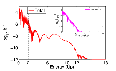
(a)  Full ATI photoelectron spectrum and interference term (inset)

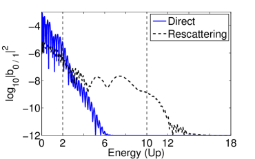
(b)  Direct and re-scattering photoelectron spectra

Figure 1: (color online) Photoelectron ATI spectra (in logarithmic scale) as a function of the ponderomotive electron energy $U_{p}$ computed by using our quasi-classical model and for each one of the transition terms: (a) Total photoelectron spectra, Eq. (15), (red line) with the interference term in the inset (magenta line). (b) Direct photoelectron spectrum $|b_{0}({p}_{z},t_{\rm F})|^{2}$ and re-scattering photoelectron spectrum $|b_{1}({p}_{z},t_{\rm F})|^{2}$ are depicted in blue solid and black dashed lines, respectively. The vertical dashed lines correspond to the classical $2U_{p}$ and $10U_{p}$ cutoffs (see the text for details).

To confirm that our model is able to capture the left-right asymmetry Milošević et al. (2006), in Fig. 2 we compute ATI spectra for electrons with positive and negative momenta along the $p_{z}$-direction. Fig. 2(a) shows the results of our quasi-classical model, meanwhile in Fig. 2(b) the TDSE in 1D is used. The photoelectrons with negative (positive) momentum are conventionally named left (right) electrons and correspondingly the photoelectron spectra associated are labeled by $|b_{\rm L}(p_{z},\phi_{0})|^{2}$ and $|b_{\rm R}(p_{z},\phi_{0})|^{2}$, respectively.

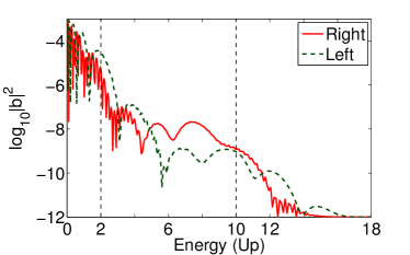
(a)  SFA Calculations

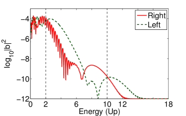
(b)  TDSE Calculations

Figure 2: (color online) Comparison of the ATI spectra for an hydrogen atom. (a) Photoelectron energy distribution (in logarithmic scale) for the emitted electrons with negative (green dark line) and positive (red line) momentum obtained by the integration of our derived full transition amplitude $|b({p_{z}},t_{\rm F})|^{2}$. (b) The same as in (a) but computed by the numerical solution of the TDSE in 1D. The vertical dashed lines correspond to the classical $2U_{p}$ and $10U_{p}$ cutoffs (see the text for details).

The photoelectron spectra computed by using the numerical solution of the TDSE in 1D, Fig. 2(b), allow us to evaluate the accuracy of our quasi-classical ATI model. The numerical integration of the TDSE is performed by using the Split-Spectral Operator algorithm Feit et al. (1982) and we use the FFTW Frigo and Johnson to evaluate the kinetic energy operator of our Hamiltonian $\hat{H}=\frac{\hat{p}_{z}^{2}}{2}+\hat{V}(z)+zE(t)$. For the present numerical solution of the TDSE, we have fixed the position grid step to $\delta z=0.2$ a.u., with a total number of points ${\rm N}_{z}=17000$. The ground state is computed via imaginary time propagation with a time step of $\delta t=-0.02\,i$ and the soft-core Coulomb potential is given by: $V(z)=-\frac{1}{\sqrt{z^{2}+a}}$. The parameter $a=2$ a.u., is chosen in such that the ground state yields the ionization potential of the hydrogen atom, i.e. $I_{p}=0.5$ a.u.

The strong-field laser-matter interaction is simulated by evolving the ground state wave function in real time, with a time step of $\delta t=0.02$ a.u., and under the action of both the atomic potential and the laser field. The laser pulse parameters are the same as those used to compute the results of Fig. 1. At the end of the laser field $t_{\rm F}$, when the electric field is zero, we compute the final photoelectron energy-momentum distribution $|b_{\rm TDSE}(p_{z},t_{\rm F})|^{2}$, by projecting the “free” electron wave packet, $\Psi_{c}(z,t_{\rm F})$, over plane waves. The wave packet $\Psi_{c}(z,t_{\rm F})$, is computed by smoothly masking the bound states from the entire wave function function $\Psi(z,t_{\rm F})$ via: $\Psi_{c}(z,t_{\rm F})=h(z)\Psi(z,t_{\rm F})$, where, $h(z)=\exp(-(\frac{z-z_{0}}{\sigma})^{2})$ is a gaussian filter.

Figure 2 demonstrates good qualitative agreement between the photoelectron spectra calculated with our quasi-classical model and those obtained by the numerical solution of the TDSE in 1D. The left-right photoelectron spectra show the expected two cutoffs defined by $2U_{p}$ and $10U_{p}$ (black dashed lines) which are present in the ATI process Lewenstein et al. (1995); Milošević et al. (2006). This shows that our approach is a reliable alternative for the calculation of ATI spectra. Our model furthermore captures the left-right dependence of the emitted photoelectrons as shown in Fig. 2(a), and in comparison with the TDSE shown in Fig. 2(b). The ability to capture this dependence and its features is especially important for applications to methods such as LIED which relies on large momentum transfers and backscattered electron distributions. For instance, photoelectrons ejected towards the left differ substantially from those emitted to the right for the case when a few-cycle driving pulse is used. According to the quasi-classical analysis of Section II, one can then infers that electron trajectories emitted towards the right have larger probability to perform backward re-scattering with the ionic core than the electrons emitted towards the left Paulus et al. (2001); Milošević et al. (2006). This behavior is clearly reproduced by both models shown in Fig. 2 and it is the basis for the stereo ATI technique developed by Paulus et al. Paulus et al. (2001).

Since our model is capable of capturing the general CEP dependence we turn to a more detailed investigation on whether our model can reproduce detailed CEP dependence by computing the ATI spectra as a function of the absolute laser phase $\phi_{0}$. Henceforth, we define the left-right asymmetry $\mathcal{A}({p_{z}},\phi_{0})$ as visibility:

$$\mathcal{A}({p_{z}},\phi_{0})=\frac{|b_{\rm L}({p_{z}},\phi_{0})|^{2}-|b_{\rm R}({p}_{z},\phi_{0})|^{2}}{|b_{\rm R}({p}_{z},\phi_{0})|^{2}+|b_{\rm L}({p}_{z},\phi_{0})|^{2}}.$$ (38)

We compute the ATI spectra for a set of CEP values between $\phi_{0}=\mp 180\degree$, and evaluate the asymmetry $\mathcal{A}({p_{z}},\phi_{0})$ of Eq. (38). The results are shown in Fig. 3. Our calculated asymmetry $\mathcal{A}({p_{z}},\phi_{0})$ shows a clear dependence on the absolute phase $\phi_{0}$, of the laser pulse. For instance, when the CEP is $\phi_{0}=\mp$ 90°, the photoelectron spectra show a left-right symmetry, which is clearly visible in the energy region between $0$ and $4U_{p}$ (see Fig. 3). This symmetry can be attributed to the direct term $\textit{b}_{0}$, which dominates the photoelectron spectra at lower energies and is a consequence of the symmetry of the electric field with respect to the envelope maximum. On the other hand, and as we shall see later, the high-energy re-scattered electrons do not follow this symmetry.

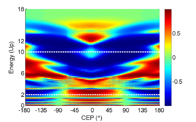
Figure 3: (color online) Asymmetry of the photoelectron energy distribution $\mathcal{A}(p_{z},\phi_{0})$ as a function of the CEP. The horizontal dashed white lines denote the $2U_{p}$ and $10U_{p}$ cutoffs rule for the direct and re-scattering photoelectrons, respectively. The laser pulse and the atomic parameters are the same that those used in Fig. 2.

For the energy range $5U_{p}\lesssim E_{p_{z}}\lesssim 12U_{p}$, the term $|b_{\rm L}|^{2}$ is less than $|b_{\rm R}|^{2}$ around $\phi_{0}=0\degree$. This implies that left electron trajectories have less probability to perform backward re-scattering than those trajectories emitted to the right. Note that this process changes if the CEP of the laser pulse is larger than $90\degree$ thereby the change is for energies between $5U_{p}\lesssim E_{p_{z}}\lesssim 8U_{p}$. In this interval the electron trajectories emitted to the left have a larger probability than the ones towards. For low-energy photoelectrons $E_{p_{z}}<5U_{p}$, the asymmetry oscillates between positive and negative values, which means that the left-right direct photoelectrons are more difficult to evaluate compared to using re-scattered ones. Thus, these results depicted in Fig. 3 clearly show that our model describes the typical dependence of the ATI spectra on the CEP Paulus et al. (2001); Milošević et al. (2006) and in particular the backward re-scattering events. Our model therefore can be used to describe the absolute phase of the driving IR laser pulse. With the purpose to understand the left-right symmetry (or asymmetry) presented in Fig. 3, we compute both the direct and re-scattering terms for two different CEP values, namely $\phi_{0}=0\degree$ and $\phi_{0}=90\degree$. The results are depicted in Fig. 4. In the case of $\phi_{0}=0\degree$ the laser pulse is asymmetric with respect to the pulse envelope maximum, i.e. it has a $\sin(\omega_{0}t)$ carrier wave. Consequently, from the phase contribution in Eq. (12) of the direct term, one can expect that the phase as a function of time is asymmetric as well. It is a consequence of the Fourier relation that a temporal asymmetry leads to an asymmetric spectral phase. In analogy, the temporal asymmetry of the phase of the direct photoelectron term, leads to the final photoelectron momentum distribution $|b_{0}(p_{z},t_{\rm F})|^{2}$ being asymmetric with respect to the momentum zero axis. This dependence is the origin of the asymmetric shape of the left-right emitted photoelectrons shown in Fig. 4(a). On the other hand, when the phase of Eq. (12) is time symmetric, which is the case of $\phi_{0}=90\degree$, i.e. the phase is proportional to $\cos(\omega_{0}t)$, we infer that the photoelectron spectrum for the direct term should be symmetric. This is exactly what we observe in the direct term which is depicted in Fig. 4(b). Moreover, in both cases the re-scattering term $|b_{1}(p_{z},t_{\rm F})|^{2}$ is asymmetric with respect to the $p_{z}=0$ momentum. Hence, from the quasi-classical analysis addressed in Eq. (17) and due to the few-cycle electric field waveform, the electron trajectories strongly depend on the CEP and the left-right momentum asymmetry is visible due to the occurrence and interference of only a few emission and re-scattering events.

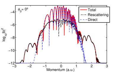
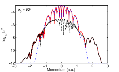
Figure 4: (color online) Left-right photoelectron momentum distributions (in logarithm scale) for the different contributions, direct term $|b_{0}(p_{z},t_{\rm F})|^{2}$ (blue dashed line), the re-scattering term $|b_{1}(p_{z},t_{\rm F})|^{2}$ (black dashed with points line), and the “total” term, $|b(p_{z},t_{\rm F})|^{2}=|b_{0}(p_{z},t_{\rm F})+b_{1}(p_{z},t_{\rm F})|^{2}$ (red solid line), to the ATI spectra for two different CEP values, $\phi_{0}=$ 0°and $\phi_{0}=$ 90°are depicted in (a) and (b), respectively. The laser pulse and the atomic parameters are the same that those used in Fig. 2.

In order to complete the analysis, we have extended our numerical calculations of the photoelectron momentum distribution for the ATI process from a 1D-momentum line to a 2D-momentum plane. In Fig. 5 we depict results for both models: our analytical quasi-classical ATI model (Fig. 5(a)) and the exact numerical solution of the TDSE in 2D (Fig. 5(b)). We find qualitative good agreement between the results of our model and the full numerical solution of the TDSE in 2D. We also find that the distribution is symmetric with respect to the $p_{y}$ axis. Note that these observations are in good agreement with calculations and measurements presented in Refs. Arbó et al. (2006); Kling et al. (2008); Wittmann et al. (2009).

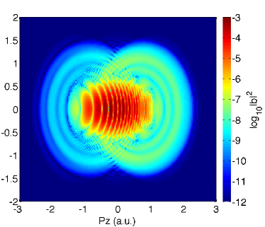
(a)  SFA calculations

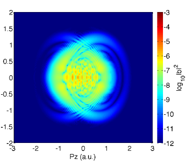
(b)  TDSE calculations

Figure 5: (color online) Comparison between our semi-classical model and the TDSE in 2D for an hydrogen system. (a)-(b) Photoelectron ATI spectra $|b(p_{z},p_{y},t_{\rm F})|^{2}$ (in logarithmic scale) computed by employing our model and the TDSE-2D numerical solution, respectively. The laser pulse parameters used in these calculations are the same as those employed in Fig 2. Note that the laser field is polarized along the $z$-direction.

The comparison shows that our quasi-classical approach can be used to model 2D-momentum distributions and even 3D-momentum distributions. However, from the contrast between the two models, we infer that our semi-analytical model is limited to photoelectrons with high energies. The origin of this discrepancy arises from the approximation made in the model with regard to the atomic potential. Statement (iii) relates to the fact that the atomic potential is neglected when the electron is born in the continuum. Hence, we expect that electrons with lower final energies are not well described by our quasi-classical approach.

Finally, the main advantage of the analytical model is shown in Fig. 6 which depicts the individual contributions to the 2D ATI spectrum, namely, the direct (Fig. 6(a)), re-scattering (Fig. 6(b)) and interference term (Fig. 6(c)), respectively. The resulting total and experimentally accessible ATI momentum spectrum $|b({p}_{z},p_{y},t_{\rm F})|^{2}$ is shown in Fig. 6(d).

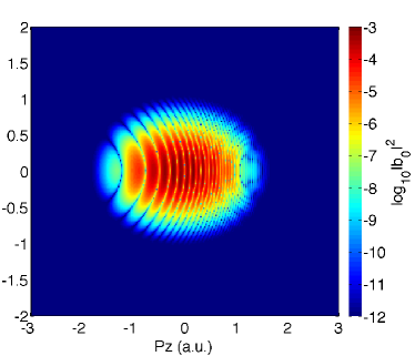
(a)  Direct Term

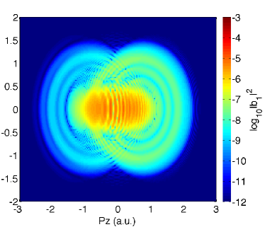
(b)  Rescattering Term

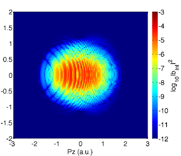
(c)  Interference Term

(d)  Total contribution

Figure 6: (color online) Different contributions to the photoelectron spectra for a 2D-momentum plane $(p_{z},p_{y})$. ATI photoelectron spectra (in logarithmic scale) as a function of the momentum $(p_{z},p_{y})$ computed by our quasi-classical model for each term. (a) Direct term, (b) re-scattering term, (c) interference term and (d) total contribution.

The atomic potential and the laser parameters used in these simulations are identical to those employed in the calculations for Figs. 1-4. Analog to the 1D calculations, the computed photoelectron momentum spectrum for the direct term (Fig. 6(a)) shows contributions for electron energies less than $2U_{p}$. We find that the contribution of the re-scattering term (Fig. 6(b)) extends to higher momentum values. Clearly visible is the symmetry of the structures about the $p_{y}$ axis for all the terms and a left-right asymmetric shape for electrons with $p_{z}<0$ or $p_{z}>0$.

We like to emphasize the importance of Eqs. (17) and (37), from which we conclude that the form of the calculated ATI spectra depends strongly on the parameters $\Gamma$ and $\gamma$ of our SR potential model. These parameters have a strong influence on the re-scattering term, which could get largely suppressed for a particular choice of them. This strong dependence suggests that the re-scattering process depends strongly on the atomic target which means that particular structural information is encoded in the ATI photoelectron spectra. Consequently the proposed semi-analytical model can be used to extract target structure and electron dynamics from measured photoelectron spectra.

V Conclusions and Outlook

We have studied the photoionization process mediated by a strong laser field interacting with an atomic system. We analyzed in detail approximate analytical solutions of the TDSE, obtained under the assumption of the strong field approximation, i.e. once an electron is tunnel ionized, its dynamics is solely governed by the driving laser, which leads to re-scattering or re-collision events. Based on this approach, we have identified and calculated the two main contributing terms in the ionization process: the direct and the re-scattering transition probability amplitudes. In addition, the bound-free dipole and the re-scattering transition matrix elements were analytically computed for a non-local potential. We stressed that this is one of the main difference of our developed model that those traditionally found in the literature for the ATI process. These analytical derivations of the re-scattering matrix element allowed us to demonstrate that the re-scattering process strongly depended on the atomic target features. A quasi-classical analysis of the re-scattering transition amplitude was performed in terms of the saddle point approximation, which permits linking the dynamics to relevant quasi-classical information, i.e. classical electron trajectories. Our analytical results suggested that the main contributions to the re-scattering transition amplitude correspond to electron trajectories, with significant probability of backward scattering off the ionic core.

Our model was used to demonstrate that both contributions, the direct and the re-scattering terms, shown left-right asymmetry depending on the carrier envelope phase of the laser pulse. This behavior has been confirmed by a comparison with the exact numerical solution of the TDSE and we found very qualitative good agreement, particularly in the high energy region of the photoelectron spectra. Apart from testing the validity of our model, we stress that it presents important advantages, such as the possibility to disentangle the effects of both the direct and re-scattered terms.

We showed also that the model is sensitive to the CEP, and by using the fact that we can investigate individual contributions to the photoelectron spectrum, we identified the re-scattering term that plays a dominant role by varying its influence based on the atomic parameters. These findings confirm that the photoelectron spectra contain structural information about the re-scattering process, i.e. about the shape of the ground state wave function, as well as the bound-free, and free-free matrix transition elements. This dependence implies that atomic structural information can be efficiently extracted with our model for methods such as LIED which measure ATI spectra.

While our aim was the establishment of a basic semi-analytical theoretical framework based on the SFA, we note that our approach is applicable to more complex, and thus more interesting systems such as molecules. The method could be extended to describe dynamically evolving molecular systems or atomic clusters. It will be interesting to corroborate which kind of information could be extracted, and whether one could visualize molecular dynamics such as vibrations or dissociation, or if the ground state molecular orbital could be reconstructed. We will address these and similar questions in future publications.